Online Track Anomaly Detection: Comparison of Different Machine Learning Techniques Through Injection of Synthetic Defects on Experimental Datasets

Abstract

The adoption of instrumented wheelsets on diagnostic trains offers the possibility of continuous monitoring of wheel–rail contact forces. The collection of large datasets can be exploited for diagnostic purposes, aiming to localize specific track defects, allowing significant improvements in terms of safety and maintenance costs. Machine learning (ML) techniques can be used to automate anomaly detection. In this work, the authors compare the application of various ML algorithms based on the identification of different frequency or time-based features of analyzed signals. To perform the activity, a significant number and variety of local defects have been included in the recorded data. From a practical point of view, the insertion of real known defects into an existing line is extremely time-consuming, expensive, and not immune to safety issues. On the other hand, the design of anomaly detection algorithms involves the usage of relatively extended datasets with different faulty conditions. The authors propose deliberately adding real contact force profiles of healthy lines to a mix of synthetic signals, which substantially reproduce the behavior and the variability of foreseen faulty conditions. The results of this work, although preliminary and still to be completed, offer a contribution to the scientific community both in terms of obtained results and adopted methodologies.

1. Introduction

Ensuring the safety, reliability, and availability of railway networks remains a continuous challenge for infrastructure managers. Traditional maintenance strategies rely on periodic onsite inspections that are often model-based as proposed by Chiachío, et. al. [1] and by Bianchi et al. [2], which are often unable to match the actual rate of track degradation. In this context, instrumented, diagnostic trains described by CIFI [3] and Mermec [4], and Track Recording Vehicles (TRV) such as the ones adopted by Rete Ferroviaria Italiana (RFI) in Italy, represent a valid solution to implement continuous monitoring, diagnostic, and prognostic-oriented activities. These trains are equipped with a large set of different and often redundant measurement systems such as the one described by Hoelz et al. [5] and Ward et al. [6].

In this work, the focus is on vertical irregularities and longitudinal levels defined according to EN13848 [7] associated with a wide variety of track defects often described in the review literature, such as that of Rosano [8].

Instrumented wheelsets (IWS) equipped with strain gauges are capable of directly measuring the contact forces exchanged at the wheel–rail interface, representing a promising and largely underexplored technology for diagnostics, mainly for two reasons:

• IWS are widely used for homologation, derailment risk assessment, and static load verification as proposed by Rigall and Santos [9], but their potential use for diagnostics and in-service condition monitoring is only proposed by pioneering works such as that of Gullers [10]. They are still much less investigated with respect to other methods.
• Inertial Measurement Sensors (Inertial Measurement Unit—IMU) are still robust and cost-effective solutions by La Palma et al. [11] and Pieringer et al. [12] to monitor wheel–track interaction with a particular attention to vertical displacements and longitudinal levels according to EN13848.

The availability of large datasets for diagnostic purposes automatically introduces a further research exigence, namely, automatically handling large amounts of data to automatically detect and track anomalies. Therefore, there is a growing interest, as stated by recent works of Tsunashima [13], Malekjafarian [14], and Ghiasi [15,16], on the application of different artificial intelligence (AI) or machine learning (ML) approaches to classify measured data and identify potential anomalies. One-Class Support Vector Machine (OCSVM) is one of the most proposed approaches for such applications by Schölkopf et al. [17]. Moreover, most of the scientific community still focuses on the analysis of inertial measurements that are probably considered cheaper to implement and maintain, and more robust for extended use for diagnostic purposes.

The possible application of ML and AI techniques for the analysis of wheel–rail contact force measurements offers promising and interesting possibilities aligned with recent research trends. Moreover, it gives the possibility of investigating a topic (the use of contact forces as a primary source of information for track conditions), which, despite its potential, is still relatively uncovered by the current technical literature.

The application of ML and AI techniques is strongly influenced by the way in which data used for both calibration and validation of the methods are preprocessed and classified. The availability of labeled data (pre-classified anomalies) enables supervised learning techniques. For the proposed application, the calibration of ML algorithms needs a large amount of data, which strongly influences the detection performance. Such data can be assured by the acquisition of relatively extended mission profiles in which faults and anomalies are represented in a statistically significant way. This necessity conflicts with maintenance and safety issues, which makes it difficult, expensive, and dangerous to introduce and tolerate some anomalies subjected to a regular commercial exercise of the line. So, collected data from regular railway traffic on well-maintained railway lines can be reasonably considered statistically free from large defects. For this reason, applicable ML approaches are substantially unsupervised or semi-supervised. The algorithm itself classifies the anomalies with respect to some criteria reflecting and exploiting some features of the recorded data.

The unsupervised anomaly detection techniques that will be compared in this work were chosen for their relatively simple implementation and wide adoption. These can be roughly classified into three categories:

• Statistical and Density-Based Methods (also Graph and Manifold-Based Approaches): such algorithms (e.g., Gaussian Mixture Models, Kernel Density estimation, Thresholding, Manifold learning, etc.) assume that normal data are statistically dense with respect to some significant features. On the contrary, anomalies are relatively distant. In manifold methods, this classification is also associated with the creation of a boundary. OCSVM [17] is probably one of the most successful and largely applied of these methods as proposed by Ghiasi et.al. [18], not only for the proposed application but more generally for solutions related to contact force classification proposed by Pires [19] or prognostics of the infrastructure according to Sresakoolkai [20];
• Distance- and Nearest-Neighbor-Based Methods: anomalies are identified as points that are distant or isolated with respect to normal ones in terms of an assigned distance metric, or with respect to some other neighboring criteria. There are several approaches (e.g., k-Nearest-Neighbors, Local Outlier Factor, or Density-Based Spatial Clustering). Local Outlier Factor (LOF) by Berunig et al. [21] is often considered a good baseline for applying such approaches to anomaly detection.
• Clustering-Based Approaches: data are artificially clustered; K-means or hierarchical clustering are typical examples, but Isolation Forest (IF) by Liu et al. [22] is probably one of the most adopted methods thanks to its robustness and relatively fast implementation and execution.

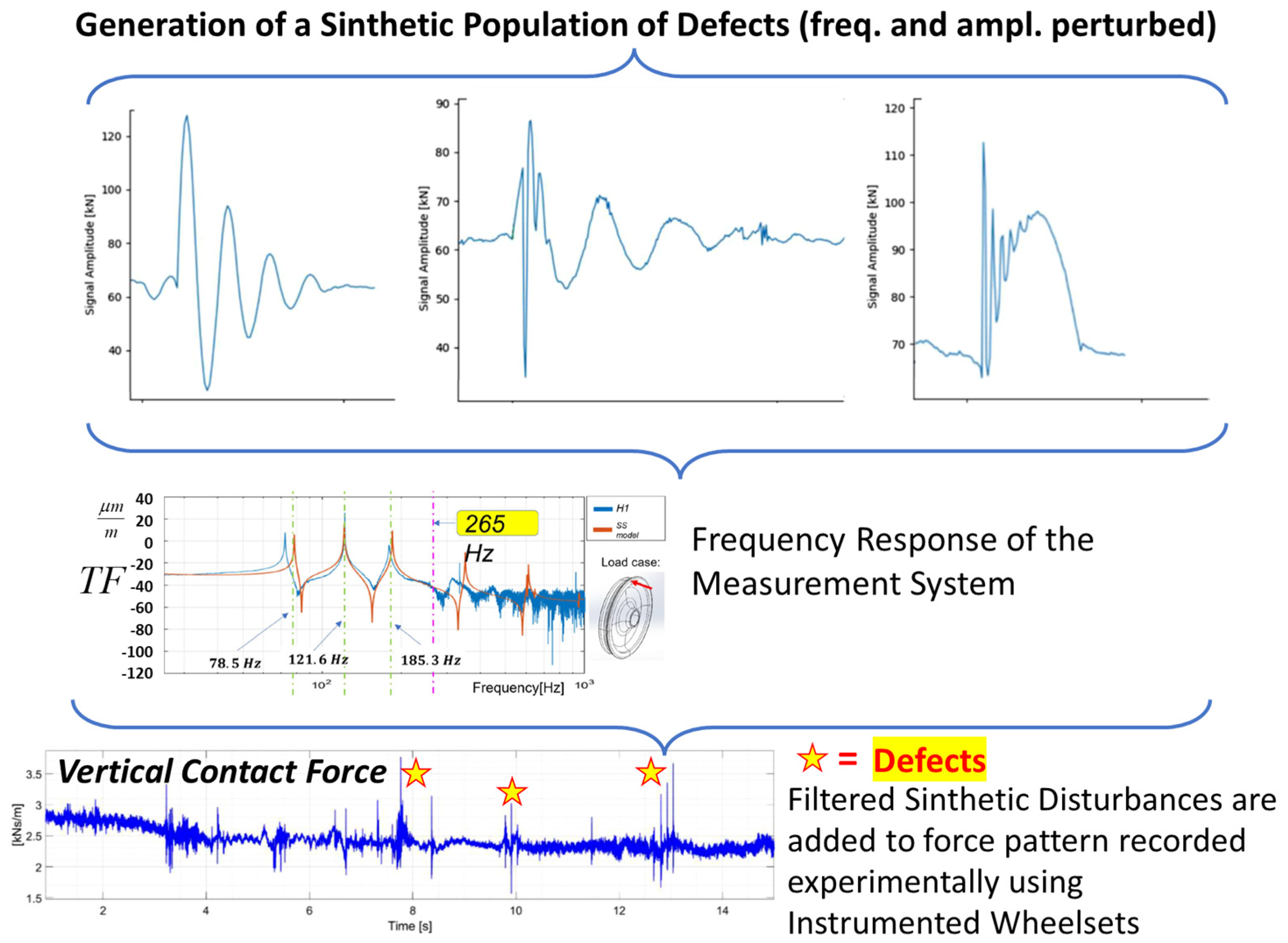
Regarding the anomalies to be detected, there is a wide literature base such as example by Hoelz et al. [23], Iwnicky [24] and Esveld [25] that describes some well-known defects and irregularities of the track head, such as squats as described by Zhao and Li [26] or dipped joints as proposed by Dukkipati and Dong [27] in terms of recorded vertical contact forces profiles, as shown in Figure 1.

Thus, it is possible to recreate synthetic force patterns that reproduce the typical behavior of the real or numerically generated effect. As a baseline for this work, artificially generated numerical defects are injected into real recorded force profiles of high-speed lines, which are reasonably considered free of defects. There are a significant number of synthetic defect patterns that are also pre-filtered to reproduce frequency response limitations or distortions associated with the adopted measurement systems. The estimated frequency response of IWS was known from previous research activities performed by the authors [28] using Python libs [29].

Once the methodology for generating artificial mission profiles with known faults was established, different ML algorithms were applied and compared:

• OCSVM;
• IF;
• LOF.

Analysis has been repeated considering different signal features with a particular distinction between statistical time- or space-sample-based features (sampled with respect to time or space, respectively) and spectral-based features calculated using the Fourier Transform (FT) or Wavelet Decomposition.

The paper is organized as follows:

• Datasets and feature calculation used for model calibration and validation, referring to a mission profile at more than 300 km/h on a high-speed line. Such data cannot be explicitly revealed since it is covered by a non-disclosure agreement with the data supplier. Only limited information can be provided.
• Application of ML algorithms to statistical space-based features.
• Application of ML algorithms to statistical frequency domain features.
• Mixed approach: ML is applied to a mixed set of features (both in the space and frequency domains).
• Final Evaluation of the results, aiming to summarize the performances of the proposed approaches.

Novelty of the proposed approach can be summarized in the following key points:

• Most of the literature regarding on-line monitoring of track quality in terms of vertical displacements is more focused on different kinds of inputs (inertial).
• The proposed methodology for the injection of artificial disturbances is quite innovative, and it is supported by a preliminary knowledge and modeling of the bandwidth achieved by the considered IWS.
• Three different ML methodologies and different signal features, both in the space and frequency domains, are compared. The proposed analysis, far from complete (research is still ongoing), still represents a good and interesting tutorial for the scientific community. This third contribution is useful for understanding the potential advantages of the proposed injected disturbances, not for the novelty of the proposed algorithms that are deliberately aligned with some of the most adopted techniques for anomaly detection.

2. Adopted Datasets for Both Calibration and Validation

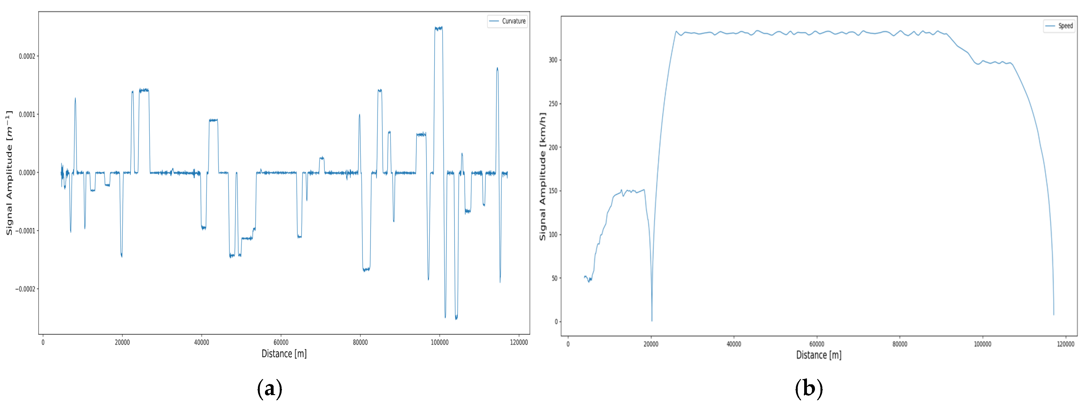
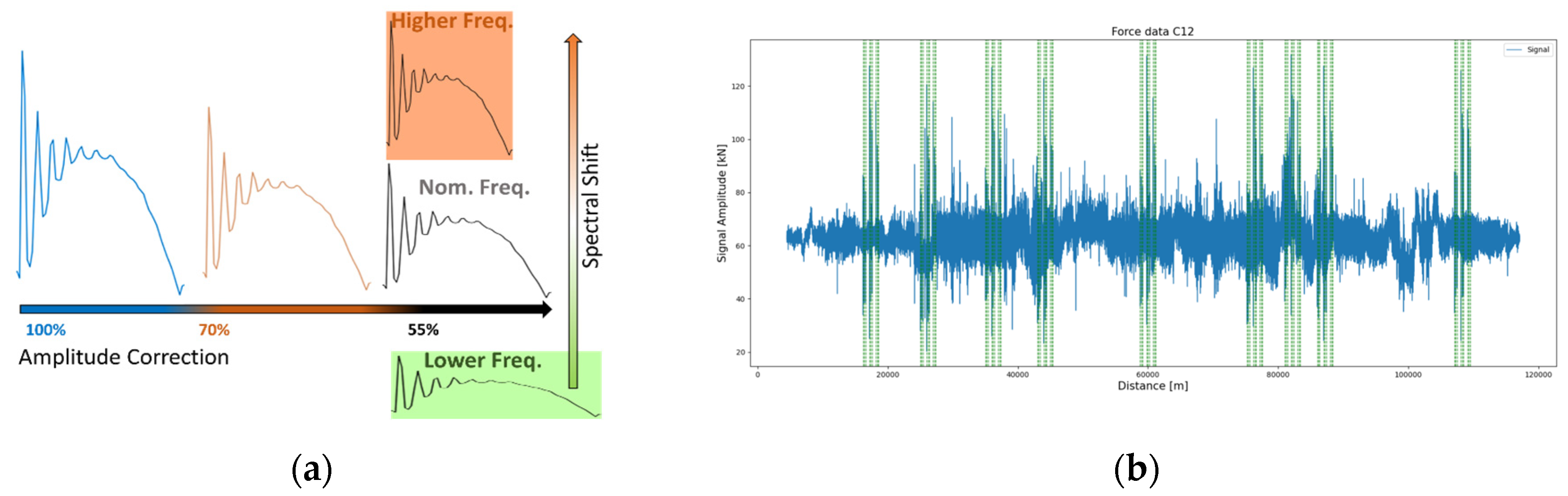
The main features of the adopted training and validation dataset are shown in

Table 1. Adopted training and validation sets.

Dataset Name	Train Max Speed and Tolerance [km/h]	Track Type	Length [km] (Duration [s]) Sampling Period [m]
C14 (Training Set)	330 ± 5	Mixed *	113.2 (2263) ** 2.5 × 10−2
C12 Validation/Fitting Set	320 ± 5	Mixed *	112.6 (2252) ** 2.5 × 10−2

* For both mission profiles: Min curv. radius 4000 [m]. Max slope 5‰; ** data are resampled with a spatial sampling of 2.5 cm, starting from data originally sampled at several kHz; for both profiles, 81 randomly distributed irregularities are introduced.

: data are referred to high-speed service as shown in Figure 2a,b, where speed and curvature profiles are associated with the training dataset, namely C14. The validation dataset force profiles are perturbed with 81 disturbances, corresponding to well-known defects such as welds, squats, and joints previously described in Figure 1. As shown in Figure 3a, disturbances are further modified by introducing amplitude and frequency scaling. This operation is performed to introduce a wider variability in the shape of anomalies that must be recognized by tested ML algorithms, stressing their robustness, which is critical in a real field application, since three different waveforms are introduced with variable amplitudes and shifted frequency contents.

In Figure 3b, the force profile perturbed by injected disturbances (marked with green vertical-dashed lines on the resulting pattern) is shown. It is interesting to notice that the shape of the signal correspondence of the injected synthetic anomalies does not differ substantially from other sections of the original signal. It can be confirmed that injected disturbances are not too easy to detect. Thus, the proposed profiles represent a significant benchmark to test the proposed ML algorithms for anomaly detection (each validation and training set is composed of about 4.5 million force measurements). Tests in Figure 2 are related to a high-speed train traveling at about 300 km/h. The diagnostic train is equipped with instrumented wheelsets.

Creation of Injected Disturbances

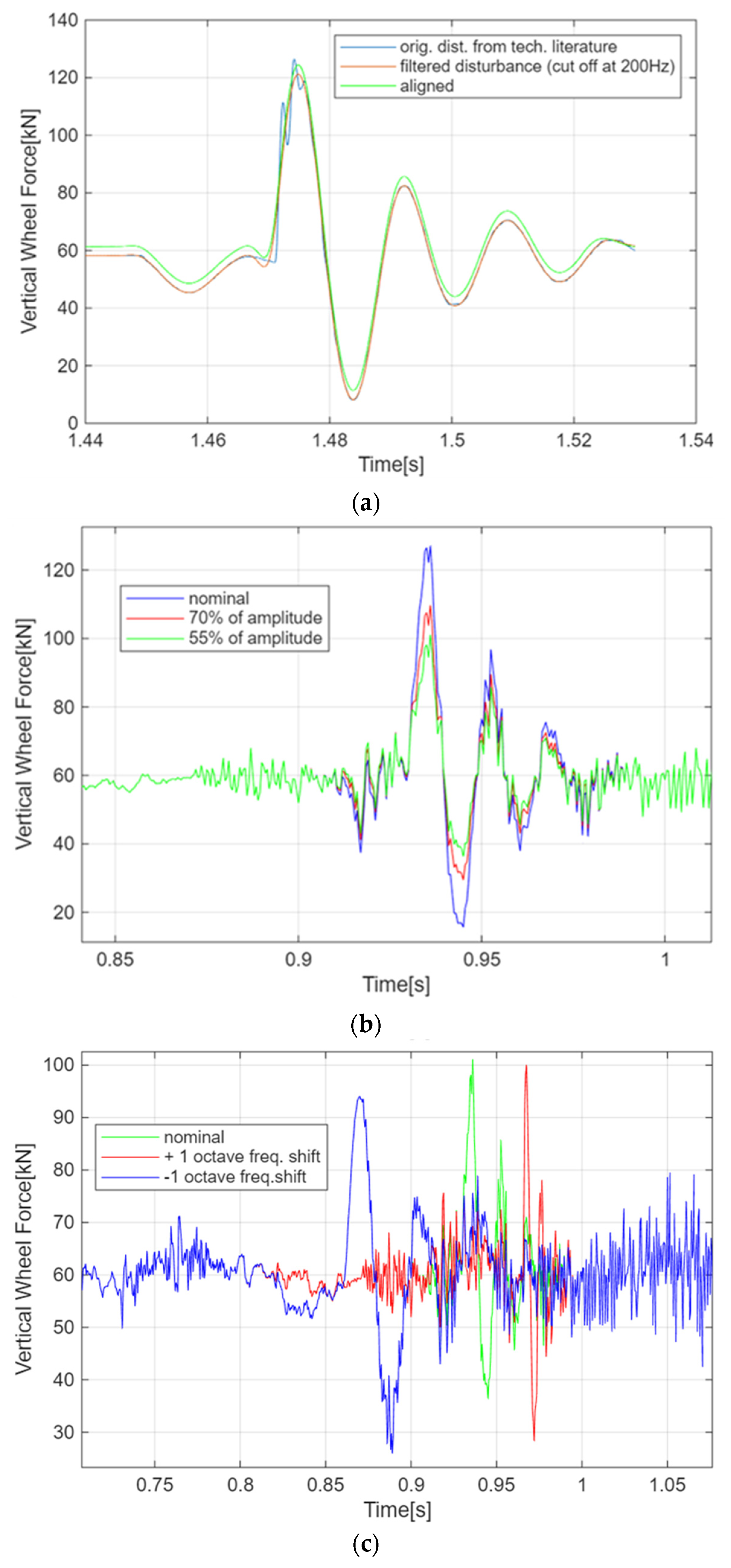
Creation of simulated-synthetic defects such as the ones represented in Figure 1, the authors have adopted the approach that is briefly described in Figure 4a–c:

• First, an irregular pattern profile is extracted from reference tech work. For example, the (a) defects that are often associated with a weld as described by Correa et al. [29], with a dip joint as introduced by Sun et al. [30] or Welds as investigated by Gao et al. [31] are digitally acquired as visible in Figure 4a.
• As shown in Figure 4a, the acquired waveform is filtered according to the cautiously estimated bandwidth of the adopted measurement system, which is assumed to be between 200 and 250 Hz, as previously estimated by the same authors [32]. Additional preprocessing features involve the subtraction of the mean force value (only force fluctuation is considered) and a windowing (a trapezoidal window is adopted) that is performed to reduce numerical discontinuities between the injected disturbance and preexisting signals.
• Then, the disturbance is directly summed to a real contact force measurement in which smaller fluctuations are associated with null or acceptable defects. In this way, high-frequency components associated with noise and unmodeled dynamics of the measurement systems are directly taken from the real measurement system.
• As shown in Figure 4b,c, the defect can be scaled to reproduce different amplitudes or stretched to shift the associated frequency content:

  ○

  Scaling, as shown in Figure 4b, is performed by simply multiplying the disturbance by an assigned factor (1, 0.7, or 0.5).

  ○

  Frequency shifting can be performed alternatively both in the time and frequency domains. As shown in Figure 4c, a spectrum shift of one octave is considered.

• Scaling and frequency shifting of injected disturbances are introduced to stress the capacity of the proposed algorithm to recognize different disturbances. The tech. literature offers a wide variety of described anomalies, but these examples are related to a wide variety of different conditions in terms of rolling stock, considered defects, and mission profiles. So, the aim of the performed scaling and frequency shifting is to introduce a wider variety of injected disturbances to test the robustness of the investigated algorithms.

3. Application of ML Algorithms to Space-Domain Features

As previously introduced, three different ML algorithms, OCSVM, IF, and LOF, have been used for anomaly detection (Novelty detection). Analysis was performed in Python (version 3.14), using the libraries listed in

Table 2. Python Libraries used for the implementation of the proposed algorithms.

Library *	Usage Description
NumPy [33]	Basic mathematical operations
SciPy [34]	Signal analysis, spectral analysis, FFT
Scikit-learn [35]	Machine learning algorithms, frameworks, classifiers, evaluation metrics
Pandas [36]	Tables and data management
Joblib [37]	Load/save datasets, data management, features, parallel computing
Tkinter [38]	GUI design
Mdf Reader [39]	Load/save datasets
Matplotlib [40]	Figure plotting
Numba [41]	High-speed parallelized feature calculation

* all update with last version 3.14 of Python.

. After several iterations, omitted for brevity, some statistical features were selected as listed in

Table 3. Extracted spatial features.

Parameter	Symbol	Formula
Mean	µ	$\mu ={\displaystyle \frac{1}{N}}{\displaystyle \sum _{i=1}^N}x\left[i\right]$
Peak value	$x_{peak}$	$max\left|x_i\right|$
RMS	RMSf	${RMS}_f=\sqrt{{\displaystyle \frac{1}{N}}{\displaystyle \sum _{i=1}^N}{\left(x_i\right)}^2}$
Skewness	${Sk}_f$	${Sk}_f={\displaystyle \frac{\frac{1}{N}{\sum }_{i=1}^N{(x_i-\mu )}^3}{{\sigma }^3}}$
Kurtosis	${Kr}_f$	${Kr}_f={\displaystyle \frac{\frac{1}{N}{\sum }_{i=1}^N{(x_i-\mu )}^4}{{\sigma }^4}}$
Superior order moments (order k = 5.6)	Ord_kf	${Ord\_k}_f={\displaystyle \frac{\frac{1}{N}{\sum }_{i=1}^N{(x_i-\mu )}^k}{{\sigma }^k}}$
Peak factor	Pkf	${Pk}_f={\displaystyle \frac{x_{peak}}{\mu }}$
Crest Factor	Crf	${Cr}_f={\displaystyle \frac{x_{peak}}{{RMS}_f}}$
Impulse factor	Impf	${Imp}_f={\displaystyle \frac{x_{peak}}{\frac{1}{N}{\sum }_{i=1}^N\left|x_i\right|}}$
Shape factor	Shf	${Sh}_f={\displaystyle \frac{{RMS}_f}{\frac{1}{N}{\sum }_{i=1}^N\left|x_i\right|}}$
Clearance Factor	Clf	${Cl}_f={\displaystyle \frac{x_{peak}}{{\left(\frac{1}{N}{\sum }_{i=1}^N\sqrt{\left|x_i\right|}\right)}^2}}$
Margin Factor	Maf	${Ma}_f={\displaystyle \frac{{Cl}_f}{{Sh}_f}}$
Mobility	MH	$M_H=\sqrt{{\displaystyle \frac{Var\left[\dot{x}\right]}{Var\left[x\right]}}}$
Complexity	CH	$C_H=\sqrt{{\displaystyle \frac{Var\left[\ddot{x}\right]/Var\left[\dot{x}\right]}{M_H}}}$

.

Let Q(s) denote the wheel–rail contact force as a function of the spatial coordinate s [m]. Space s is integrated from speed v according to (1).

The raw time-series signal Q(t), mapped to space using (1), is resampled on a uniform spatial grid (2) where ∆s is the sampling distance.

$$s\left(t\right)={\int }_0^{t}v\left(\tau \right)d\tau ,\hspace{1em}\hspace{1em}\hspace{1em}\hspace{1em}\left(Q\left(s\right)=Q\left(t\left(s\right)\right)\right),$$

(1)

$$s_n=n∆s,\hspace{1em}\hspace{1em}\hspace{1em}\hspace{1em}\left(n=0, \dots , N-1\right).$$

(2)

Feature extraction is performed over overlapping spatial windows of length Lw = NΔs (Each window is tapered with a suitable weighting function w[n] (Hann with unit energy) to reduce spectral leakage.

$$x_w\left[n\right]=x\left[n\right]w\left[n\right],\hspace{1em}\hspace{1em}\hspace{1em}\hspace{1em}\left(n=0, \dots , N-1\right)$$

(3)

Additionally, Hjorth parameters as described by Oh et al. [42], also listed in Table 3, are used. Hjorth parameters provide a compact description of a signal’s variability and frequency content and have shown potential in condition-monitoring applications. Given a windowed signal x[n], let $\dot{x}$[n] and $\ddot{x}$[n] denote its first and second discrete derivatives. Defining the variance operator as Var[⋅], the Hjorth parameters of mobility and complexity are defined according to formulas also shown in Table 3. Compared ML algorithms are calibrated with respect of the metrics defined in Equations (4)–(6), functions of statistical performances of the algorithms in terms of identified anomalies, classified in True Positives (TP), defined as correctly identified signal windows with Ground Truth (GT) anomalies; False Positives (FP), healthy windows misclassified as defective; False Negatives (FN), missed/unrecognized anomalies; True Negatives (TN), properly recognized healthy data points.

$$Precision={\displaystyle \frac{TP}{TP+FP}}$$

(4)

$$Recall={\displaystyle \frac{TP}{TP+FN}}$$

(5)

$$F1score=2·{\displaystyle \frac{Precision·Recall}{Precision+Recall}}$$

(6)

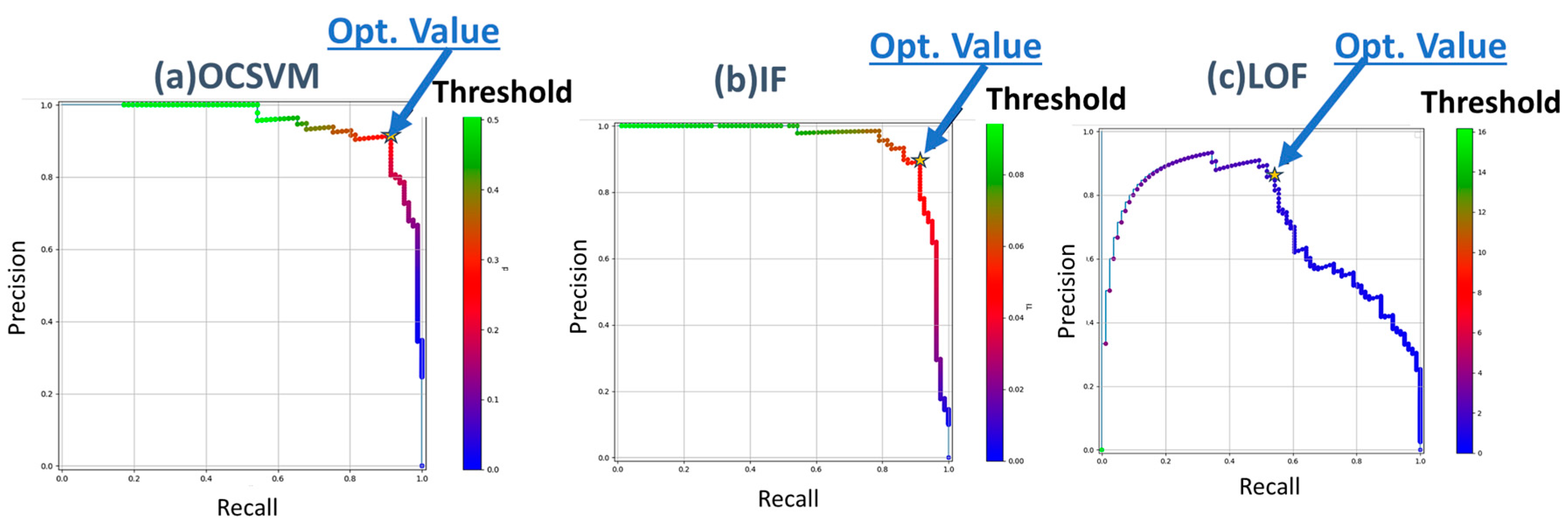
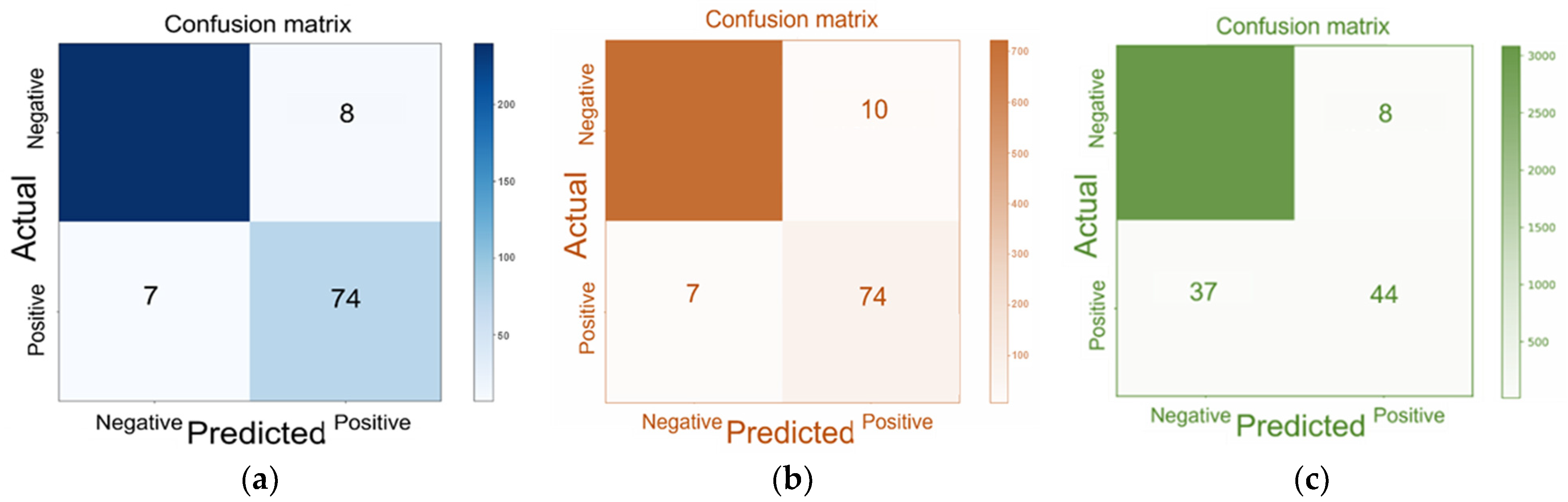
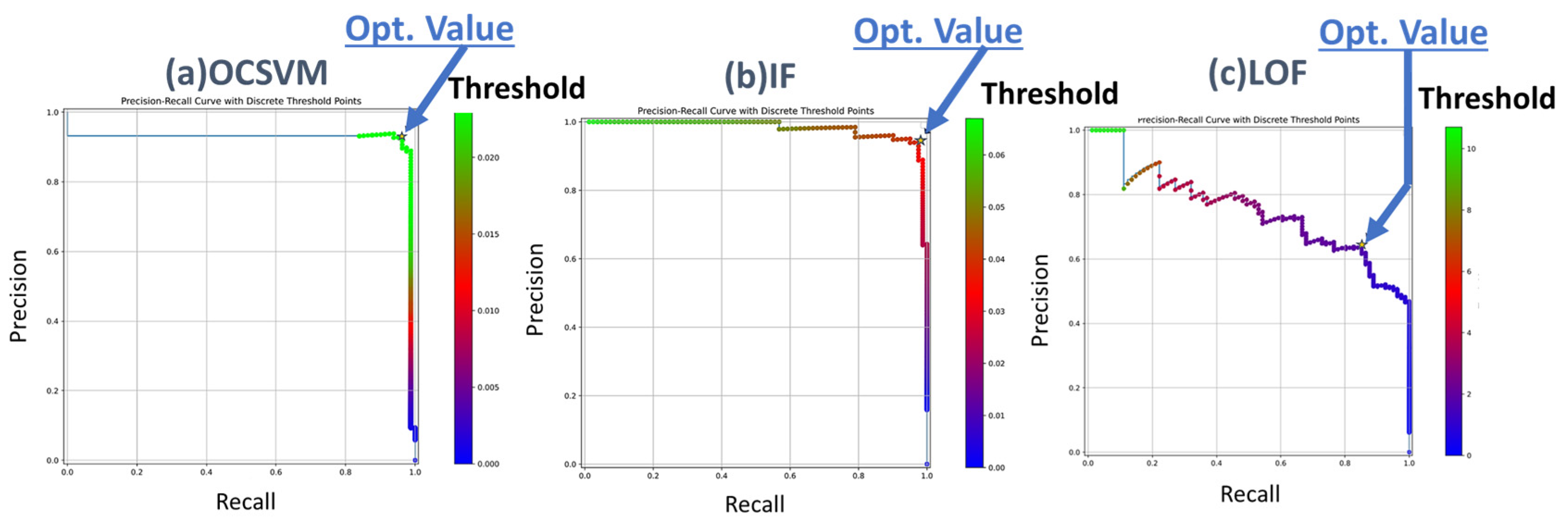
The results of calibrated OCSVM, IF, and LOF are shown in

Table 4. Classifier comparison and detection performance summary (Space domain).

Classifier	Retrieved Instances	Optimal F1-Score	Optimal Precision	Optimal Recall	Time Performance
OCSVM 1 (Threshold 0.24)	TP: 74/81 FP: 8 FN: 7 Max TP: 81	0.914	0.902	0.914	Training: 180 s Fitting: 136 s
IF 2 (Threshold 0.051)	TP: 74/81 FP: 10 FN: 7 Max TP: 81	0.897	0.881	0.914	Training: 249 s Fitting: 23 s
LOF 3 (Threshold 1.6)	TP: 44/81 FP: 8 FN: 37 Max TP: 81	0.667	0.846	0.543	Training: 6540 s Fitting: 13,200 s

Adopted hyper-parameters for Classifiers: OCSVM ¹: ν = 10⁵ (reciprocal of regularization/anomaly fraction); γ = 0.01 (kernel width); kernel: RBF (Radial Basis Function kernel); L_W = 50 (window length); Scaling: Robust; Overlapping 90%; IF ²: n_estim = 1000 (number of isolation trees in the forest); Contamination = 0.001; L_W = 50 (window length); Scaling: Standard; Overlapping 90%; LOF ³: Neighbors = 200 (Number of nearest-neighbors used to compute the local density), Contamination = 2 × 10⁻⁵ (expected fraction of anomalies), L_W = 50 (window length); Scaling: Standard; Overlapping 90%.

, in Figure 5, and in Figure 6a–c. As expected, none of the chosen algorithms can properly detect all the injected irregularities. For OCSVM, the inclusion of fifth- and sixth-order statistical moments significantly improved detection accuracy, with all other parameters held constant (signal windowing, scaling method, etc.). Conversely, the Hjorth parameters proved highly effective in the case of IF, resulting in a substantial reduction in FP and an increase in TP. By comparing the classifiers under their respective optimal configurations, which is given by the adoption of the decision function threshold that maximizes a selected metric (e.g., F1 score), it was determined that OCSVM achieved the best detection performance. It outperformed LOF and showed superior accuracy compared to IF. On the other hand, IF demonstrated the fastest training and inference times among the three classifiers. Regarding LOF, performances at least for the purpose of this work seem to be less interesting. Hyperparameters adopted for the calibration of each algorithm are listed at the bottom of the table. Parameter optimization was performed using a grid search approach (simulations are repeated with different sets of hyperparameters until a reasonable optimization is reached). The results of the iteration procedure in terms of chosen thresholds for the three investigated algorithms are shown in Figure 5.

4. Results

Spectral analysis is a fundamental approach for signal investigation, with the Short-Time Fourier Transform (STFT) being widely used for analyzing non-stationary signals whose frequency content changes over time. Unlike the traditional Fourier Transform, which gives only global frequency information, the STFT divides a signal into short, overlapping segments using a sliding window (e.g., Hann or Hamming). A Fourier Transform is computed for each segment, producing a time-localized frequency spectrum. Stacking these spectra generates a spectrogram image, where time (or space), frequency (or wavenumber), and spectral intensity are plotted on two axes and color, respectively. This representation allows tracking spectral evolution over time (or space), which is particularly useful in applications such as vibration analysis and condition monitoring. The STFT, however, involves a trade-off between time and frequency resolution: shorter windows improve time resolution but reduce frequency resolution, and vice versa. Despite this, its simplicity and clarity make it a key tool for analyzing transient or time-varying phenomena, such as contact forces. A similar approach makes use of wavelet decomposition/transforms as previously described in this work of Bellacci et al. [43].

Rather than analyzing the entire waveform directly, each windowed segment was represented by a set of descriptive statistics that are briefly listed in

Table 5. Extracted spectral features.

Parameter	Symbol	Formula
Spectral Centroid	Cs	$C_s={\displaystyle \frac{{\sum }_k{f}_k{\left|X\left[k\right]\right|}^2}{{\sum }_k{\left|X\left[k\right]\right|}^2}}$
Spectral Spread	Ss	$S_s=\sqrt{{\displaystyle \frac{{\sum }_k{\left(f_k-C_s\right)}^2{\left|X\left[k\right]\right|}^2}{{\sum }_k{\left|X\left[k\right]\right|}^2}}}$
Spectral Skewness	Sks	$S_{ks}={\displaystyle \frac{{\sum }_k{\left(f_k-C_s\right)}^3{\left|X\left[k\right]\right|}^2}{{S_s}^3{\sum }_k{\left|X\left[k\right]\right|}^2}}$
Spectral Kurtosis	Ks	$K_s={\displaystyle \frac{{\sum }_k{\left(f_k-C_s\right)}^4{\left|X\left[k\right]\right|}^2}{{S_s}^4{\sum }_k{\left|X\left[k\right]\right|}^2}}$
Spectral Crest Factor	CFs	$C_{Fs}={\displaystyle \frac{max\left(\left|X\left[k\right]\right|\right)}{\sqrt{\frac{1}{N}{\sum }_k{\left|X\left[k\right]\right|}^2}}}$
Spectral Flatness	SFs	$S_{Fs}={\displaystyle \frac{{\left({\prod }_k\left|X\left[k\right]\right|\right)}^{\frac{1}{N}}}{\sqrt{\frac{1}{N}{\sum }_k\left|X\left[k\right]\right|}}}$
Band-Energy Ratios	Eb	$E_b={\displaystyle \sum _k}{\left|X\left[k\right]\right|}^2$

.

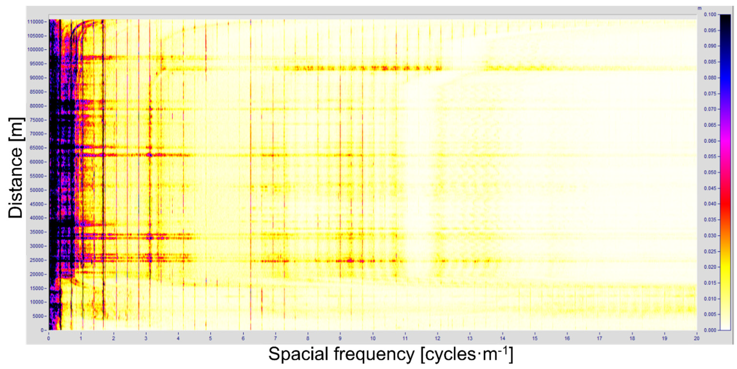
The data (the same datasets described in Table 1) were processed using a band-pass filter within the wavenumber range 0.1–15.625 [cycles/m]. The lower cut-off was selected to ensure the interpretability of the spectrogram, following a preliminary Fourier analysis. As shown in Figure 7, it was observed that, below a certain threshold, it becomes difficult to effectively distinguish relevant spectral features.

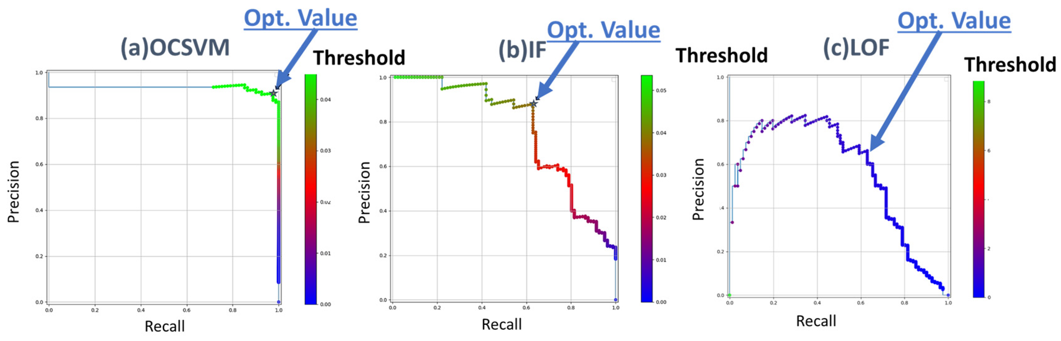
The same three anomaly detection algorithms (OCSVM, IF, and LOF) are then calibrated using the frequency features of Table 5. The obtained calibration results are shown in

Table 6. Classifiers comparison and detection performance summary (frequency domain).

Classifier	Retrieved Instances	Optimal F1-Score	Optimal Precision	Optimal Recall	Time Performance
OCSVM 1 (Threshold 0.045)	TP: 79/81 FP: 9 FN: 2 MaxTP: 81	0.940	0.898	0.975	Training: 877 s Fitting: 1150 s
IF 2 (Threshold 0.038)	TP: 51/81 FP: 8 FN: 30 MaxTP: 81	0.734	0.864	0.630	Training: 127 s Fitting: 195 s
LOF 3 (Threshold 0.60)	TP: 59/81 FP: 30 FN: 22 MaxTP: 81	0.698	0.663	0.728	Training: 5840 s Fitting: 8910 s

Adopted hyper-parameters for Classifiers: OCSVM ¹: ν = 10⁵ (reciprocal of regularization/anomaly fraction); γ = 0.01 (kernel width); kernel: RBF (Radial Basis Function kernel); L_W = 50 (window length); Scaling: Robust; Overlapping 90%; IF ²: n_estim = 1000 (number of isolation trees in the forest); Contamination = 0.001; L_W = 50 (window length); Scaling: Standard; Overlapping 90%; LOF ³: Neighbors = 200 (Number of nearest-neighbors used to compute the local density), Contamination = 2 × 10⁻⁵ (expected fraction of anomalies), L_W = 50 (window length); Scaling: Standard; Overlapping 90%.

. Also, in Figure 8, the iterative calibration of the thresholds for the three investigated algorithms is shown.

The length Lw of the moving window used for feature calculation did not exhibit a consistent influence on detection performance, unlike in the case of statistical space-domain features. For all classifiers, the general trend observed for OCSVM indicated an increase in the maximum number of detected TPs with decreasing Lw (using the default decision function threshold > 0). However, when using the optimal threshold, selected to maximize the F1-score, the number of detected TPs decreased steadily. This suggests that the algorithm retrieves a larger number of positive instances (outliers) as Lw decreases, but most of them correspond to FPs with higher decision-function values than true anomalies. Contrary to initial expectations, shorter signal windows did not compromise the information captured by the FFT. No significant loss of spectral characteristics was observed when smaller Lw values were used. Based on the results, OCSVM remains the most promising classifier for novelty detection of rail-head faults, followed by IF and LOF. Despite the much smaller number of features used for anomaly detection with respect to the previous test case, OCSVM exhibits relatively good performance. From a computational point of view, the analysis of frequency-related features is numerically intensive. Increased computational effort can be attributed not only to the STFT process, requiring FFT computation for each signal window, which is inherently time-consuming, but also to limitations in parallelization: the STFT step cannot be executed within the Numba parallel computing framework, as it is incompatible with the FFT modules in SciPy and NumPy. Considering these critical aspects of implementation, there is a high probability of improvements in the feature if such libraries are updated.

Hyperparameters adopted for the calibration of each algorithm are listed at the bottom of the table. Parameter optimization was performed using a grid search approach (simulations are repeated with different sets of hyperparameters until a reasonable optimization is reached).

5. Application of ML Algorithms Considering a Mixed Set of Frequency- and Space-Domain Features of Measured Contact Forces

Comparison between ML algorithms is finally repeated considering the analysis of both statistical space features and frequency features, respectively described in Table 3 and Table 5. The results of the model fitting are shown in

Table 7. Classifiers comparison and detection performance summary (combined approach with spatial- and frequency-based features).

Classifier	Retrieved Instances	Optimal F1-Score	Optimal Precision	Optimal Recall	Time Performance
OCSVM 1 (Threshold 0.023)	TP: 78/81 FP: 6 FN: 3 MaxTP: 81	0.945	0.929	0.963	Training: 2590 s Fitting: 2443 s
IF 2 (Threshold 0.043)	TP: 79/81 FP: 6 FN: 2 MaxTP: 81	0.952	0.930	0.975	Training: 230 s Fitting: 219 s
LOF 3 (Threshold 1.70)	TP: 69/81 FP: 40 FN: 12 MaxTP: 81	0.730	0.633	0.851	Training: 7760 s Fitting: 16,060 s

Adopted hyper-parameters for Classifiers: OCSVM ¹: ν = 10⁵ (reciprocal of regularization/anomaly fraction); γ = 0.01 (kernel width); kernel: RBF (Radial Basis Function kernel); L_W = 50 (window length); Scaling: Robust; Overlapping 90%; IF ²: n_estim = 1000 (number of isolation trees in the forest); Contamination = 0.001; L_W = 50 (window length); Scaling: Standard; Overlapping 90%; LOF ³: Neighbors = 200 (Number of nearest-neighbors used to compute the local density), Contamination = 2 × 10⁻⁵ (expected fraction of anomalies), L_W = 50 (window length); Scaling: Standard; Overlapping 90%.

. Also, in Figure 9, the iterative procedure used to calibrate the threshold adopted for the three investigated algorithms is shown.

The adoption of combined features involves an augmented computational load. The best performing and fastest algorithm proved to be the IF one. However, the results of IF with combined features are comparable to the corresponding performances of OCSVM when only frequency features are considered, at least when the most performing algorithm (OCSVM) is considered.

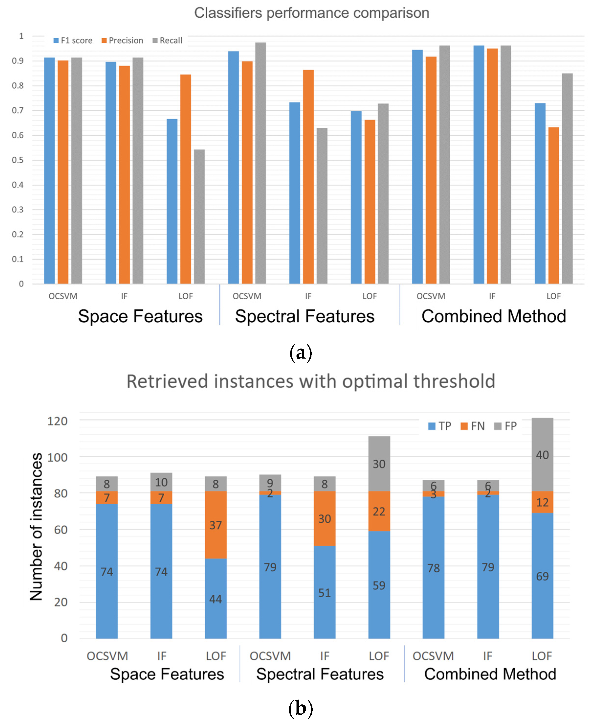
More generally, the usage of frequency-related features seems to bring benefits, lowering the number of FP instances, raising the related performance metrics (Precision, Recall, and F1 score). The higher performance of IF with the mixed set of features makes it preferable (in the present case) to OCSVM. Such consideration seems to be largely justified by the results summarized in Figure 10a,b, where all the tested configurations are compared.

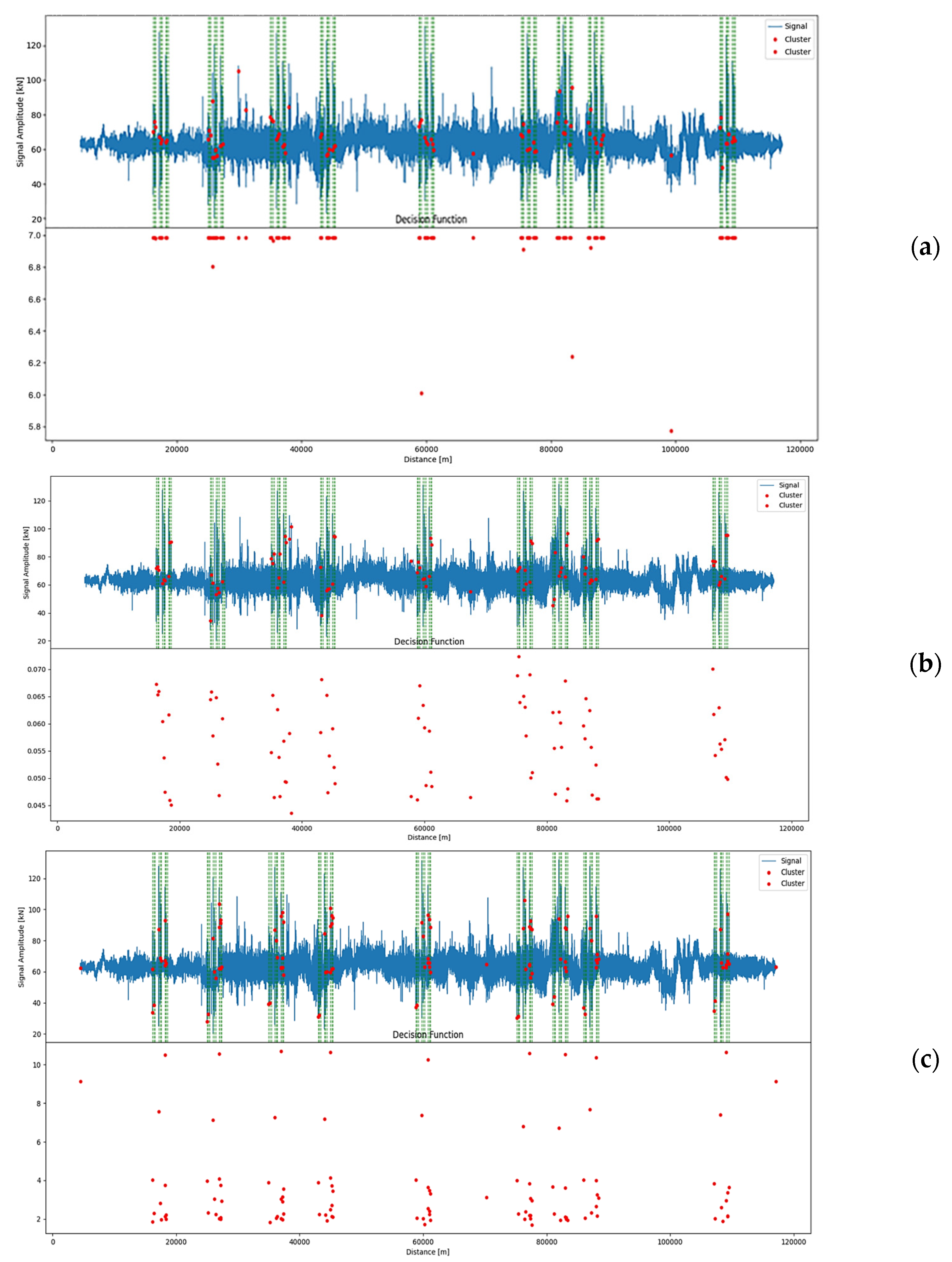
It is interesting to note that at least two or three injected anomalies are not always properly recognized by the most performing algorithms, and the quantity of FN remains consistent. The reason is quite simple: these are the injected disturbances with the lowest amplitude and the most shifted spectrum. Thus, this small low-frequency disturbance imposes contact force fluctuations with patterns associated with normal behavior. An example of classifier outlier-detection output is finally shown in Figure 11. This comparison shows that the OCSVM has proven to be quite easy to calibrate with respect to the other tested algorithms.

Hyperparameters adopted for the calibration of each algorithm are listed at the bottom of the table. Parameter optimization was performed using a grid search approach (simulations are repeated with different sets of hyperparameters until a reasonable optimization is reached).

Critical Evaluation of Obtained Results in Terms of Recorded False Positive and False Negative Estimations

Looking at the preliminary results shown in this work, it is noticeable that there is a residual population of wrong classifications (False Positives and False Negatives), which is very small but not null. This result cannot be explained by a suboptimal calibration of chosen algorithms (at least for OCSVM and IF). So, authors have investigated the limited number of samples in which the performed anomaly detection fails; this result is interesting: every False Negative estimation is associated with injected disturbances with reduced amplitudes and reduced frequency content (spectrum shifted down by 1 octave). Anomaly scores associated with these False Negative classifications are quite near the chosen thresholds.

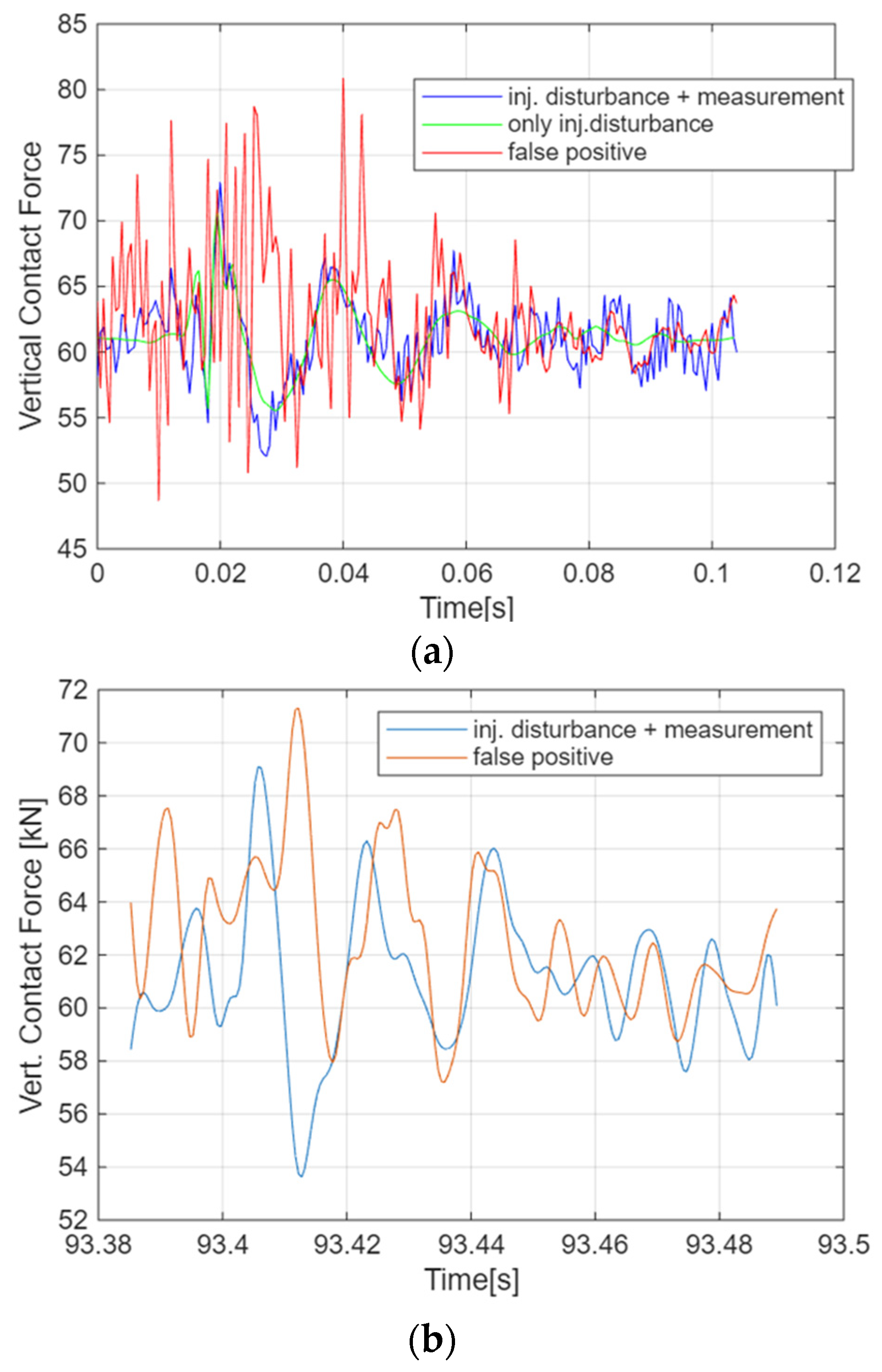
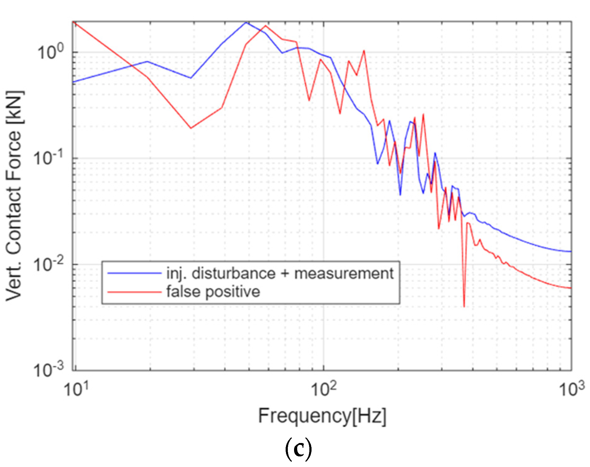
Otherwise, False Positive estimations are associated with experimental samples for which the presence of some very small defect that is normally not considered is at least feasible or probable. An example in this sense is represented by the comparison of an experimental signal, which is classified as a False Positive, with an injected disturbance that is classified as a True Positive. In 12/a, three curves are compared: the measured force with synthetic injected disturbance, the pure injected disturbance (that is summed to the force pattern), and finally the real measurement classified as False Positive. Profiles are quite similar.

As shown in Figure 12b,c, if both signals are filtered at 200 [Hz], the bandwidth for which is considered more reliable is the adopted measurement system. The comparison of force patterns both in the time and frequency domains is even more similar. So, there is a clear indication that the pattern classified as False Positive is probably a small defect that is normally tolerated because it is still too small to be detected or to be potentially harmful for railway exercise, also considering that recorded patterns are referred to a train traveling at about 300 km/h.

This also shows that some of the smallest defects that are injected in this study are near this minimum sensitivity level, which corresponds to small acceptable irregularities that are physiological, even on a well-maintained line.

So, these results give interesting indications:

• The shape of a very small disturbance, not deliberately introduced in the measurement, is quite similar to an injected disturbance. This is a partial indirect validation of the proposed method to inject disturbances into a real measurement pattern.
• The proposed system, even when performing wrong classification (a False Positive Anomaly), identifies something that has at least the probability of being classified or evolving in the future into a defect. Comparison with further inspection systems normally installed on Italian diagnostic trains can help to refine the classification of recorded anomalies. Results confirm the choice of integrating multiple measurement technologies on Italian diagnostics [2] as the right one.
• The limitation of the proposed approach is not the algorithm, but the usage of only one class for the detection of anomalies. The adoption of multiple classes aiming to classify detected anomalies also in terms of severity should probably be the right choice to recognize hard anomalies for which intervention is mandatory, with respect to light anomalies that should eventually be mapped for further evolutionary analysis of the line state. So, it is not only a trivial question of refining the calibration of ML algorithms but also of improving the engineering know-how associated with the definition of defects that should be recognized.

6. Conclusions and Future Development

In this work, the authors have proposed and investigated the application of different ML algorithms for the detection of anomalies in terms of local short-wavelength irregularities of recorded measurements of vertical contact forces Q, measured with an IWS.

Preliminary results are promising, although obtained on a relatively small dataset with artificially generated disturbances, are quite interesting, exploring a topic that is relatively under-investigated by the current scientific literature. Authors are working on the further extension of the proposed method to other kinds of rolling stock and to other mission scenarios, both in terms of performed mission profiles and defects recorded or injected on the line.

However, authors believe that thanks to the increasing diffusion of diagnostic rolling stock equipped with IWS, this kind of measurement could gain increasing favor in Italy and more generally in Western Europe.

Currently, the authors are continuing to work on this topic, focusing their attention on these possible improvements:

• Field validation: conducting extensive measurement campaigns to correlate anomalies with verified track defects, providing robust GT for model and ML validation.
• Anomaly Classification in Multiple Classes: performed activities have demonstrated that the classification of anomalies with multiple classes related at least to severity should be useful to better manage the maintenance actions that should be accomplished according to the detection of an anomaly. This approach should also be useful for improving the way in which detected anomalies are managed by those responsible for maintenance.
• Advanced spectral analysis: Integrate Wavelet or Empirical Mode Decomposition (EMD) with Hilbert-Huang transform to improve transient resolution and complement the limitations of the STFT.
• Feature selection and explanation: Implement interpretability-driven approaches (e.g., SHAP, LIME, ANOVA) to identify the most informative features contributing to fault detection. As far as this activity is concerned, some preliminary investigations have been carried out; however, the authors have been currently delayed in favor of a more articulated identification of anomalies with multiple classes.
• RMS and mean in the figure, retaining only one representative from each group.
• Real-time deployment: Explore edge-computing or cloud-assisted implementations to enable on-board real-time monitoring and decision support for maintenance operations.
• Synergy with inspection drones: recent developments of VTOL drones proposed by Pugi et al. [44] offer the possibility of interesting synergies with diagnostic rolling stock equipped with IWS. The drone, as proposed by Cardellichio et al. [45], can automatically reach areas in which defects are detected by the IWS, giving the possibility of rapid verification before human intervention.

References

1. Chiachío, J.; Chiachío, M.; Prescott, D.; Andrews, J. A knowledge-based prognostics framework for railway track geometry degradation. Reliab. Eng. Syst. Saf. 2019, 181, 127–141. [Google Scholar] [CrossRef]
2. Bianchi, G.; Fanelli, C.; Freddi, F.; Giuliani, F.; La Placa, A. Systematic review of railway infrastructure monitoring: From classic techniques to predictive maintenance. Adv. Mech. Eng. 2025, 17, 1–26. [Google Scholar] [CrossRef]
3. CIFI. La Diagnostica Mobile e le Misure per la Certificazione. Webinar. 31 January 2022. Available online: https://www.cifi.it/UplDocumenti/Roma31012022/Presentazione%20Bonafe_Palmiotto%20CIFI%202022-01-31.pdf (accessed on 7 January 2025).
4. MERMEC Group. I Rotabili di RFI—Il Treno Archimede. Available online: https://www.mermecgroup.com/press-room/media-coverage/420/i-rotabili-di-rfi-iltreno-archimede.php (accessed on 7 January 2025).
5. Hoelzl, C.; Dertimanis, V.; Landgraf, M.; Ancu, L.; Zurkirchen, M.; Chatzi, E. On-board monitoring for smart assessment of railway infrastructure: A systematic review. In The Rise of Smart Cities: Advanced Structural Sensing and Monitoring Systems; Elsevier Inc.: Amsterdam, The Netherlands, 2022; pp. 223–259. [Google Scholar] [CrossRef]
6. Ward, C.P.; Weston, P.F.; Stewart, E.J.C.; Li, H.; Goodall, R.M.; Roberts, C.; Mei, T.X.; Charles, G.; Dixon, R. Condition Monitoring Opportunities Using Vehicle-Based Sensors. Proc. Inst. Mech. Eng. Part F J. Rail Rapid Transit 2011, 225, 202–218. [Google Scholar] [CrossRef]
7. EN 13848-3:2021; Railway Applications. Track. Track Geometry Quality Measuring Systems. Track Construction and Maintenance Machines. International Heavy Haul Association: Minneapolis, MN, USA, 2021.
8. Rosano, G.; Massini, D.; Bocciolini, L.; Zappacosta, C.; Di Gialleonardo, E.; Somaschini, C.; La Paglia, I.; Pugi, L. Diagnostics of the railway track-Possibility of development through the measurement of accelerations and contact forces [La diagnostica dell’armamento ferroviario-Possibilità di sviluppo attraverso la misura di accelerazioni e forze di contatto]. Ing. Ferrov. 2024, 79, 81–102. [Google Scholar] [CrossRef]
9. Riggall, G.; Santos, G.F.M. Use of IWS to determine best bogie configuration for Vale under 37.5 tonne axle loads. In Proceedings of the 2011 International Heavy Haul Association Conference, Calgary, AB, Canada, 19–22 June 2011; pp. 1–9. [Google Scholar]
10. Gullers, P.; Dreik, P.; Nielsen, J.C.O.; Ekberg, A.; Andersson, L. Track Condition Analyser: Identification of Rail Rolling Surface Defects, Likely to Generate Fatigue Damage in Wheels, Using Instrumented Wheelset Measurements. Proc. Inst. Mech. Eng. Part F J. Rail Rapid Transit 2010, 225, 1–13. [Google Scholar] [CrossRef]
11. La Paglia, I.; Di Gialleonardo, E.; Facchinetti, A.; Carnevale, M.; Corradi, R. Acceleration-based condition monitoring of track longitudinal level using multiple regression models. Proc. Inst. Mech. Eng. Part F J. Rail Rapid Transit 2023, 238, 479–488. [Google Scholar] [CrossRef]
12. Pieringer, A.; Kropp, W. Model-Based Estimation of Rail Roughness from Axle Box Acceleration. Appl. Acoust. 2022, 193, 108760. [Google Scholar] [CrossRef]
13. Tsunashima, H. Condition Monitoring of Railway Tracks from Car-Body Vibration Using a Machine Learning Technique. Appl. Sci. 2019, 9, 2734. [Google Scholar] [CrossRef]
14. Malekjafarian, A.; Sarrabezolles, C.-A.; Khan, M.A.; Golpayegani, F. A machinelearning-based approach for railway track monitoring using acceleration measured on an inservice train. Sensors 2023, 23, 7568. [Google Scholar] [CrossRef]
15. Ghiasi, R.; Malekjafarian, A. Monitoring of railway tracks maintenance needs using dynamic responses collected by an in-service train. Railw. Eng. Sci. 2025, 33, 553–580. [Google Scholar] [CrossRef]
16. Ghiasi, R.; Malekjafarian, A. A data-driven framework for detecting railway maintenance needs using acceleration data collected from passing trains. In Transport Transitions: Advancing Sustainable and Inclusive Mobility; TRA Conference 2024, Lecture Notes in Mobility; McNally, C., Carroll, P., Martinez-Pastor, B., Ghosh, B., Efthymiou, M., Valantasis-Kanellos, N., Eds.; Springer: Cham, Germany, 2025. [Google Scholar] [CrossRef]
17. Schölkopf, B.; Platt, J.C.; Shawe-Taylor, J.; Smola, A.J.; Williamson, R.C. Estimating the support of a high-dimensional distribution. Neural Comput. 2001, 13, 1443–1471. [Google Scholar] [CrossRef]
18. Ghiasi, R.; Arslan, K.M.; Sorrentino, D.; Diaine, C.; Malekjafarian, A. An unsupervised anomaly detection framework for onboard monitoring of railway track geometrical defects using one-class support vector machine. Eng. Appl. Artif. Intell. 2024, 133, 108167. [Google Scholar] [CrossRef]
19. Pires, A.; Mendes, G.; Santos, G.; Dias, A.; Santos, A. Indirect identification of wheel rail contact forces of an instrumented heavy haul railway vehicle using machine learning. Mech. Syst. Signal Process. 2021, 160, 107806. [Google Scholar] [CrossRef]
20. Sresakoolchai, J.; Kaewunruen, S. Prognostics of unsupported railway sleepers and their severity diagnostics using machine learning. Sci. Rep. 2022, 12, 6064. [Google Scholar] [CrossRef]
21. Breunig, M.M.; Kriegel, H.-P.; Ng, R.T.; Sander, J. LOF: Identifying density-based local outliers. In Proceedings of the 2000 ACM SIGMOD International Conference on Management of Data; ACM: New York, NY, USA, 2000; pp. 93–104. [Google Scholar] [CrossRef]
22. Liu, F.T.; Ting, K.M.; Zhou, Z.H. Isolation forest. In 2008 Eighth IEEE International Conference on Data Mining (ICDM); IEEE: Piscataway, NJ, USA, 2008; pp. 413–422. [Google Scholar] [CrossRef]
23. Hoelzl, C.; Dertimanis, V.; Landgraf, M.; Ancu, L.; Zurkirchen, M.; Chatzi, E. Chapter 9-onboard monitoring for smart assessment of railway infrastructure: A systematic review. In The Rise of Smart Cities; Amir, H., Alavi, M., Feng, Q., Jiao, P., Sharif-Khodaei, Z., Eds.; Butterworth-Heinemann: Oxford, UK, 2022; pp. 223–259. [Google Scholar]
24. Iwnicki, S.; Spiryagin, M.; Cole, C.; McSweeney, T. (Eds.) Handbook of Railway Vehicle Dynamics, 2nd ed.; CRC Press: Boca Raton, FL, USA, 2019. [Google Scholar]
25. Esveld, C. Modern Railway Track, 3rd ed.; MRT-Productions: Warszawa, Poland, 2017. [Google Scholar]
26. Zhao, X.; Li, Z.; Dollevoet, R. The vertical and the longitudinal dynamic responses of the vehicle–track system to squat-type short wavelength irregularity. Veh. Syst. Dyn. 2013, 51, 1918–1937. [Google Scholar] [CrossRef]
27. Dukkipati, R.V.; Dong, R. The dynamic effects of conventional freight car running over a dipped-joint. Veh. Syst. Dyn. 1999, 31, 95–111. [Google Scholar] [CrossRef]
28. Bellacci, G.; Pugi, L.; Baldanzini, N. Validation of a Wheelset Finite Element Model for Static Structural Analysis and Inverse Force Identification; Lecture Notes in Networks and Systems, 1124 LNNS; Springer: Berlin/Heidelberg, Germany, 2024; pp. 236–244. [Google Scholar] [CrossRef]
29. Correa, N.; Vadillo, E.G.; Santamaria, J.; Blanco-Lorenzo, J. On the non-proportionality between wheel/rail contact forces and speed during wheelset passage over specific welds. J. Sound Vib. 2018, 413, 79–100. [Google Scholar] [CrossRef]
30. Sun, Y.Q.; Cole, C.; Spiryagin, M. Study on track dynamic forces due to rail short-wavelength dip defects using rail vehicle-track dynamics simulations. J. Mech. Sci. Technol. 2013, 27, 629–640. [Google Scholar] [CrossRef]
31. Gao, J.; Zhai, W.; Guo, Y. Wheel–rail dynamic interaction due to rail weld irregularity in high-speed railways. Proc. Inst. Mech. Eng. Part F J. Rail Rapid Transit 2018, 232, 249–261. [Google Scholar] [CrossRef]
32. Bellacci, G.; Neri, F.; Pugi, L.; Giachetti, A.; Barlacchi, E.; Baldanzini, N. Preliminary Frequency Response Analysis of a Contact Force Measurement System for Rail Applications; Lecture Notes in Electrical Engineering, 1110 LNEE; Springer: Berlin/Heidelberg, Germany, 2024; pp. 139–145. [Google Scholar] [CrossRef]
33. Numpy Library. Available online: https://numpy.org/ (accessed on 5 April 2026).
34. Scipy Library. Available online: https://scipy.org/ (accessed on 5 April 2026).
35. Scikit-Learn Library. Available online: https://scikit-learn.org/stable/index.html (accessed on 5 April 2026).
36. Pandas Library. Available online: https://pandas.pydata.org/ (accessed on 5 April 2026).
37. Joblib Library. Available online: https://pypi.org/project/joblib/ (accessed on 5 April 2026).
38. TKinter Library. Available online: https://docs.python.org/3/library/tkinter.html (accessed on 5 April 2026).
39. MDF Reader Library. Available online: https://pypi.org/project/mdfreader/ (accessed on 5 April 2026).
40. Matplotlib Library. Available online: https://matplotlib.org/ (accessed on 5 April 2026).
41. Numba Compiler. Available online: https://numba.pydata.org/ (accessed on 5 April 2026).
42. Oh, S.-H.; Lee, Y.-R.; Kim, H.-N. A novel EEG feature extraction method using Hjorth parameter. Int. J. Electron. Electr. Eng. 2014, 2, 106–110. [Google Scholar] [CrossRef]
43. Bellacci, G.; Baldanzini, N.; Pugi, L. On the Use of Wavelet Analysis for the Detection and Position Estimation of Short Wavelength Rail Head Faults. Mech. Mach. Sci. 2025, 180, 588–595. [Google Scholar] [CrossRef]
44. Pugi, L.; Mela, A.; Reatti, A.; Casazza, A.; Fiorenzani, R.; Mattei, G. A fixed wing UAV with VTOL capabilities: Design, control and energy management. Int. J. Model. Identif. Control 2022, 41, 206–221. [Google Scholar] [CrossRef]
45. Cardellicchio, A.; Faccini, L.; Nitti, M.; Renò, V.; Tarsitano, D.; Zappa, E. Enhancing railway infrastructure monitoring using hybrid VTOL drones: A case study on inspection and surveillance using custom YOLOv12 object detector. In Multimodal Sensing and Artificial Intelligence for Sustainable Future; SPIE: Bellingham, WA, USA, 2025; Volume 13570, pp. 203–210. [Google Scholar]
Figure 1. Proposed method for the injection of synthetic defects in experimental records.
Machines 14 00424 g001
Figure 2. (a) Curvature; (b) Speed profiles of the training dataset.
Machines 14 00424 g002
Figure 3. (a) Amplitude and spectral shift are introduced by scaling the signal with respect to the duration in the space domain; (b) corresponding behavior of the validation dataset (fitting) in terms of vertical forces Q after the injection of disturbances.
Machines 14 00424 g003
Figure 4. (a) Extraction and pre-filtering of defects from the literature; (b) example of amplitude scaling; (c) example of frequency shifting by one octave.
Machines 14 00424 g004
Figure 5. Iterative calibration process of the thresholds of the three proposed algorithms when only space domain features are used.
Machines 14 00424 g005
Figure 6. Confusion matrices of the calibrated (a) OCSVM; (b) IF; (c) LOF classifiers.
Machines 14 00424 g006
Figure 7. STFT of the C14 training dataset.
Machines 14 00424 g007
Figure 8. Calibration process in terms of thresholds for the three investigated algorithms when frequency domain features are exploited.
Machines 14 00424 g008
Figure 9. Calibration process in terms of thresholds for the three investigated algorithms when both space and frequency domain features are exploited.
Machines 14 00424 g009
Figure 10. Final Comparison of different ML algorithms in terms of (a) F1 score, Precision, and Recall; (b) number of TP, FN, and FP instances.
Machines 14 00424 g010
Figure 11. Classifiers outlier-detection output (considering combined spatial and frequency features): (a) OCSVM (threshold: 0.023); (b) IF (threshold: 0.043); (c) LOF (threshold: 1.70).
Machines 14 00424 g011
Figure 12. (a) Comparison of a synthetic anomaly detected as True Positive, compared with a pattern classified as False Positive, and corresponding comparison in the time (b) and frequency (c) domains considering a limited bandwidth of 200 [Hz] (3rd-order filter of Butterworth).
Machines 14 00424 g012aMachines 14 00424 g012b