Regenerative–Frictional Brake Blending in Electric Vehicles Considering Energy Recovery and Dynamic Battery Charging Limit: A Reinforcement Learning-Based Approach

Abstract

This paper presents the design, development, and evaluation of a Reinforcement Learning (RL)–based torque-split controller for the regenerative braking system (RBS) in battery electric vehicles (BEVs). The controller employs a Deep Deterministic Policy Gradient (DDPG) agent to distribute the braking demand between regenerative and frictional braking systems with the aim of maximizing energy recovery while adhering to the physical and operational constraints. To capture the charging limitation of the battery, a State-of-Power (SoP) calculation mechanism is incorporated, providing a time-varying bound on the regenerative charge power. The agent is trained in a MATLAB/Simulink environment representing the digital twin of a BEV drivetrain, and considers a mix of different braking scenarios, i.e., light braking, medium braking, hard braking, and emergency braking. The RL’s reward shaping promotes efficient utilization of the SoP-limited regenerative capability while discouraging constraint violations and aggressive control behavior. Across a range of State-of-Charge (SoC) conditions and driving cycles, including the Worldwide Harmonized Light–Vehicle Test Procedure (WLTP) and synthetic random-rich driving cycle, the RL controller consistently delivers promising performance, yielding energy recovery of up to ~98% of the total braking energy available on WLTP type 3 driving cycle while being able to operate closely to the battery SoP limit. The results demonstrate the proposed controller’s capability for adaptive, constraint-aware energy management in BEVs and underline its potential for future intelligent braking strategies.

1. Introduction

The accelerating global transition toward electric mobility has intensified the need for improvements in vehicle efficiency. Although battery electric vehicles (BEVs) eliminate tailpipe emissions, their overall energy efficiency depends on how effectively energy is recovered and utilized during operation. One of the mechanisms contributing to this efficiency is regenerative braking, in which the traction motor operates as a generator to convert the BEV’s kinetic energy into electrical energy during deceleration, thereby recharging the battery and extending driving range [1]. Research shows that regeneration can improve the energy efficiency by about 10% for some BEVs [2].

However, since in practice both frictional and regenerative braking should be engaged in parallel, achieving optimal braking torque split leads to a complex control problem. This is because the regenerative braking system (RBS) must simultaneously satisfy several competing objectives: ensuring safe and stable deceleration, maintaining braking comfort, maximizing energy recovery, and protecting battery health [1]. Existing BEVs rely on rule-based strategies to coordinate the torque split between regenerative and hydraulic braking systems [3]. While these approaches are robust and straightforward to certify, they depend on fixed calibration parameters, rendering their adaptability limited. As operating conditions change, due to variations in battery conditions, road gradient, vehicle load, etc., such controllers may become suboptimal or overly conservative, resulting in energy recovery opportunities being missed [4]. Thus, regeneration is often restricted prematurely, leaving a substantial amount of potentially recoverable energy unused [4]. Research shows that transitioning from conventional control strategies (e.g., rule-based or proportional–integral (PI) controllers) to more predictive or optimized braking strategies can increase energy recuperation by approximately 5–10% [1]. Even improvements within this range translate directly into increased effective driving range and reduced charging frequency—two factors closely tied to user confidence and acceptance of BEVs [5]. Consequently, there is growing interest in adaptive control methods capable of responding to dynamic conditions while honoring strict safety and physical constraints. In the following, a brief review of the state-of-the-art (SotA) is provided.

Fuzzy logic offers an alternative early approach, valued for its ability to encode expert knowledge and inherent robustness to nonlinear dynamics. Improvements in energy recovery of 20–30% have been reported using fuzzy logics [6,7]. A hybrid approach combining fuzzy logic and sliding mode control (SMC) in RBS has also been explored in [8], yielding energy recovery improvements of up to 6%. However, fuzzy systems are generally constrained by their manual design process since the membership functions and rule sets can be crafted only by experts. In addition, fuzzy logic cannot evaluate or optimize long-horizon performance metrics due to poor generalization to unseen conditions. Early artificial intelligence (AI) approaches focused on supervised learning, particularly the use of artificial neural networks (ANNs) [1]. In these studies, networks were trained on labeled datasets containing variables such as vehicle speed, driver demand, battery State-of-Charge (SoC), and road gradient to estimate optimal regenerative-braking torque. Although these models demonstrated improved energy recovery compared with conventional rule-based systems, they rely on extensive labeled datasets covering a wide range of operating conditions and produce purely reactive torque commands. Because they lacked any mechanism for sequential decision-making, these controllers could not account for longer-term dependencies related to how battery status evolves and/or regarding the cumulative energy recovery. Reinforcement Learning(RL) marked a methodological shift by framing the torque-allocation problem as one of optimizing cumulative reward over time. Rather than imitating labeled data, RL agents can learn braking strategies through interaction with an environment, capturing the long-term effects of each torque decision on battery SoC, vehicle dynamics, etc. Early RL research used discrete-action algorithms such as Q-learning and deep Q-networks (DQNs), which demonstrated energy-recovery gains of up to 13% [9]. However, discrete formulations inherently constrain performance by quantizing braking torque, limiting smoothness, and preventing fine-grained adjustments essential for comfort and stability. In addition, the DQN-based approach misses the battery power-limit awareness. To partly address the continuous action control, later work adopted RL algorithms such as Deep Deterministic Policy Gradient (DDPG) [10], Twin Delayed DDPG [11], and Soft Actor–Critic (SAC) [12]. These methods output real-valued torque commands and have been shown to capture the nonlinear motor–battery interactions more effectively. Hybrid approaches that combine multiple techniques have also emerged, such as fuzzy Q-learning [13] and ANN-assisted model reference controllers [14]. These systems generally achieve smoother braking transitions and enhanced adaptability. More recent studies have further expanded the scope of regenerative braking research. For instance, Chao Yang et al. [15] provide a comprehensive review of RBSs, highlighting the growing importance of integrated energy management and battery-aware control strategies, which are not explicitly addressed in earlier RL-based studies. In contrast, Jiajun Wu et al. [16] propose a multi-objective RL framework based on Munchausen Prioritized Experience (MPE)-SAC, focusing on balancing energy recovery and battery degradation. This approach focuses on long-term battery optimization through an empirical lifetime model. However, it does not consider safe dynamic power limits in the RBS control problem. In [17], a hierarchical controller is proposed in which a higher-level strategy ensures the vehicle’s stability, while a lower-level strategy handles torque allocation for energy conservation. Similarly, this approach does not consider battery power limits in problem formulation.

While early research demonstrates promising results for applying AI in RBS control, a key gap remains in the explicit handling of constraints related to vehicle and battery safety. Regenerative braking introduces large pulse currents that can lead to battery overcharging or excessive heating, causing damage and degradation. It is thus critical to handle regeneration with care, especially as battery service life increases make them more vulnerable to stressed spike charging. Our paper builds on the premise that RL can effectively learn an optimal brake–torque split that simultaneously ensures energy recovery and battery safety. This premise is grounded in RL’s inherent capability for optimal sequential decision-making, which aligns well with the structure of the control problem: each brake control action affects the BEV and battery states, which, in turn, influence subsequent decision steps. Accordingly, we design and train an RL agent that autonomously learns the optimal torque-split decisions based on experience and feedback from a BEV drivetrain model, considered as the drivetrain digital twin and developed in MATLAB/Simulink 2025b environment. We further incorporate physical limits, battery constraints, and powertrain dynamics into the learning process, and we demonstrate that doing so enables the agent to more effectively enhance regenerative braking performance under varied and time-varying operating conditions. As an additional contribution, the paper provides a thorough examination of the requirements, constraints, safety considerations, and operational limitations that govern braking. To avoid overstating novelty, this study does not claim novelty in the use of RL per se for regenerative braking or algorithmic optimization, e.g., as in [16]. Rather, the main novelty lies in the way we formulate the RL agent to blend regenerative and frictional braking in an RBS with a series configuration to be able to recover as much energy within the safe limits of battery power, which can be autonomously learned by the RL agent. This approach ensures battery safety and lifetime optimization, which is critical due to frequent spike-like charge currents during braking.

The rest of the paper is organized as follows: Section 2 presents the problem analysis related to the BEV brake system together with underlying principles, limitations, and strategies. Section 3 describes the modeling process, including electro-mechanical subsystems of the BEV, as well as the RBS control unit. In Section 4, the problem formulation and details of the proposed methodology are provided. Section 5 includes the training and testing procedures for the proposed method, along with a discussion of the results. Section 6 is dedicated to a discussion of limitations of the proposed implementation, which then ends with a presentation of the potential future research lines and our future research plan. Finally, Section 7 concludes the paper.

2. Problem Analysis

Electric traction machines used in BEVs are inherently bidirectional: they operate as motors when delivering torque to the wheels, and as generators during braking, converting mechanical energy back into electrical energy, upholding the following equation:

$$P=T_m\cdot {\omega }_m$$

(1)

where P is the power at the motor shaft (assumed ‘+’ in motoring and ‘–’ in generating mode), $T_m$ is the motor torque, and ${\omega }_m$ is the motor’s angular velocity. The BEV satisfies the total braking demand through a combination of regenerative and frictional braking, as follows:

$$T_{\mathrm{req}}=T_{\mathrm{regen}}+T_{\mathrm{fric}}$$

(2)

where T_req is the total brake torque demand, T_regen is the regenerative braking torque contribution, and T_fric is the friction brake torque. Regenerative braking can be achieved by either a parallel combination or a series combination with frictional braking. Parallel regenerative braking operates the electric motor and disk brakes simultaneously. In contrast, series regenerative braking prioritizes the electric motor first to maximize energy recovery before engaging frictional brakes, which are only applied when there is insufficient regeneration possibility (e.g., high brake demand, low vehicle speed, or fully charged batteries). Parallel regenerative braking is safer and simpler to control and offers higher reliability [1]. In this paper, we thus focus on a parallel regenerative braking strategy. The brake electronic control unit (ECU) allocates the torque split dynamically based on the vehicle’s state, battery conditions, and other factors pertaining to comfort or safety. Conventional rule-based logic relies on fixed thresholds to divide torque between T_regen and T_fric. For example, regeneration may be disabled/suppressed when the battery is in a high SoC or is cold (regenerative charging at low temperature accelerates degradation), friction braking is prioritized under strong braking demand, and regenerative braking is gradually reduced at low vehicle speeds (due to low-amplitude of the motor internal voltages). These deterministic rules, while ensuring critical safety limits, lack the ability to adapt to dynamic/changing conditions. To achieve realistic problem formulation, some practical considerations should be taken into account, as described in the following subsections.

2.1. Braking Mode Transitions

Actual RBSs typically implement different operating modes based on brake intensity, often expressed as a normalized deceleration demand $Z_N$ [18]. It is defined as the division between the requested deceleration a_required and the maximum achievable deceleration a_max. Typical thresholds are provided below [18]:

• Low Braking Intensity (Z_N < 0.5): RBS provides most or all braking torque, maximizing energy recovery.
• Moderate Braking Intensity (${0.5\le Z}_N\le 0.8$): As braking intensity increases, frictional braking is progressively introduced to supplement RBS, ensuring that deceleration demand and stability requirements are met [19].
• High/Emergency Braking Intensity ($Z_N>0.8$): Frictional braking dominates to ensure rapid deceleration; RBS is minimized or disabled [18].

The braking intensity $Z_N$ determines which mode is active. This guarantees that emergency braking is never limited by motor or battery constraints.

2.2. Operating Constraints and Considerations on RBS

The instantaneous maximum regenerative torque is also constrained by multiple factors:

• Vehicle Speed Limitations: At low BEV speeds, e.g., <~15 km/h, the motor back-electromotive force (back-EMF) is insufficient to drive current into the battery; thus, only frictional braking can be used [20]. This low-speed cutoff is a fundamental physical limitation and appears explicitly in blended braking strategies.
• Motor Speed and Power Constraints: Maximum motor brake torque T_max depends on motor speed n. Below the rated speed n_rated, the machine operates in a constant-torque region with a torque of T_max,rated, while above the rated speed, it operates in a constant-power region; thus, torque decreases inversely with the following speed [21]:

  $$T_{\max }(n)=\left\{\begin{array}{ll}{T}_{\max ,\mathrm{rated}}\hfill & n\le n_{\mathrm{rated}}\hfill \\ {\displaystyle \frac{9550P_{\mathrm{rated}}}{n}}\hfill & n>n_{\mathrm{rated}}\hfill \end{array}\right.$$

  (3)

  In the context of regenerative braking, this torque–speed characteristic directly limits how much braking torque can be produced electrically at a given vehicle speed and, thus, how much of the demanded deceleration can be covered by regeneration rather than friction.
• Battery SoC Restrictions: When the battery SoC exceeds ~90–95% [22], the Battery Management System (BMS) significantly restricts/blocks charging current to prevent overcharge damage [23]. Regenerative braking should usually be disabled in this range.
• Battery Temperature Constraints: Cold temperatures reduce ionic conductivity and slow lithium intercalation kinetics, which significantly limit charge acceptance. As documented in [24], regenerative charging power must be reduced when the cell temperature falls below ~5–10 °C to avoid lithium plating. At the opposite extreme, temperatures above ~50 °C (chemistry dependent) increase the risk of accelerated degradation and thermal instability; thus, the BMS similarly restricts charge current in high-temperature conditions.
• Vehicle Dynamics and Wheel Slip: The braking force distribution must ensure wheel slip remains within the safe bounds (~10–20%) to maintain adhesion and stability [25]. The adhesion utilization coefficient must satisfy:

  $${\mu }_i={\displaystyle \frac{F_{X,i}}{F_{Z,i}}}\le {\mu }_{\mathrm{road}}$$

  (4)

  where ${\mu }_i$ is the adhesion utilization coefficient for wheel i, representing the ratio of longitudinal braking force to the normal load, $F_{X,i}$ is the longitudinal (braking) force acting on wheel i, $F_{Z,i}$ is the normal (vertical) load on wheel i, and ${\mu }_{road}$ is the maximum road–tire friction coefficient available under current surface conditions. When Anti-lock Braking System (ABS) intervention is required, regenerative braking is overridden to ensure stability [25].
• Driver Comfort: Driver comfort in RBS is typically assessed through limits on deceleration (~2.5 $\mathrm{m}/{\mathrm{s}}^2$ in normal braking) and jerk (~3 $\mathrm{m}/{\mathrm{s}}^3$), which helps ensure smooth and predictable braking [26]. Transitions between regenerative and friction braking can challenge these limits when motor torque decreases suddenly due to low speed or battery constraints.

2.3. Safety and Regulatory Requirements for BEV Braking Systems

Existing braking systems are designed with the principle that braking functionality must never be compromised (UN Regulation 13-H). This calls for several critical considerations, including but not limited to the following:

• Redundancy: Multiple independent braking pathways ensure that single-point failures do not eliminate braking capability [27].
• Deterministic Fallback: The system must always revert to a safe state (mechanical braking) if any active control subsystem malfunctions, as mandated in brake-by-wire safety guidelines [28].
• Conservative Operation: When safety and energy efficiency conflict, safety always takes priority. Production regenerative braking strategies, therefore, prioritize hydraulic braking during uncertainty, ABS operation, or fault conditions.
• Predictable Behavior: Drivers and surrounding vehicles must be able to reliably predict deceleration behavior. Regulatory frameworks (UNECE Regulation 13-H) prescribe strict limits on variability in braking response (UN Regulation 13-H).

In current systems, regenerative braking is a secondary enhancement to the primary mechanical braking system, but never a replacement. This architectural choice simplifies safety assurance: if regenerative capability becomes unavailable due to the limits reviewed before, the vehicle still decelerates safely through hydraulic braking. Rule-based controllers exploit this hierarchy, enabling regeneration only when mechanical braking can immediately take over if regeneration is insufficient. These safety requirements explain the conservative nature of existing RBSs, which causes occasional regeneration opportunities to be missed. With the help of advanced control methods, as we also propose in this paper, it is possible to push the RBS to its full limit, making the most of the available regeneration power while closely adhering to safety requirements.

2.4. Considerations Related to the Battery Energy Storage

Regenerative braking imposes short high-power charging pulses that intensify electrochemical and thermal stress on the lithium-ion batteries (LIBs), thereby accelerating their degradation. Therefore, it is crucial to respect LIB constraints related to the SoC, State-of-Health (SoH), SoP, and temperature. Attempting to recharge a low-SoH cell or a high-SoC cell can lead to overcharging, excessive cell heating or hotspots, and potential cell failure. In the proposed approach, such dynamic conditions related to the battery are taken into account in the RBS.

To concentrate the paper on the RL part and its feasibility in the braking context, we try to simplify modeling aspects only to the most necessary components/aspects. In this paper, comfort is discussed only at a conceptual level, as the simplified drivetrain and actuator models do not permit realistic estimation of deceleration or jerk. In Section 3, a simplified drivetrain model is developed to use as a digital twin for the design of the RBS control mechanism. The simplified model reduces computational burden, which is essential given that the simulations span long-duration driving cycles.

3. BEV and RBS Modeling

This section develops a simulation-efficient electric drivetrain model for forming the physical backbone for all subsequent RBS controller design. The Section therefore proceeds in a layered manner. Section 3.1 defines the modeling requirements. Section 3.2 introduces a generic BEV architecture containing the driver, motor controller, motor–inverter block, vehicle body, and battery-related subsystems. Section 3.3 then specializes this template to a commercial BEV, namely Škoda Enyaq iV 80 (Mladá Boleslav, Czech Republic), by providing available manufacturer data, derived parameters, and calibration procedures, as well as evaluation against key performance figures of the reference vehicle.

3.1. Modeling Requirements

A set of minimum requirements is defined for the drivetrain model. The objective is to capture the dominant energy flows and actuator limits that affect braking performance while avoiding unnecessary complexity, as this will increase runtime during the AI training part. The following components and effects are thus represented explicitly in the model:

• Electric traction motor with operation in both motoring and generating modes.
• Battery system with representation of charging power limitations.
• Friction brake system capable of providing the remaining brake torque when regenerative capacity is insufficient or unavailable.
• Equivalent inertial load representing the vehicle mass at the wheels.
• Road load and environmental resistances acting on the wheels, including aerodynamic drag, rolling resistance, viscous (speed-proportional) friction, and slope or road grade.

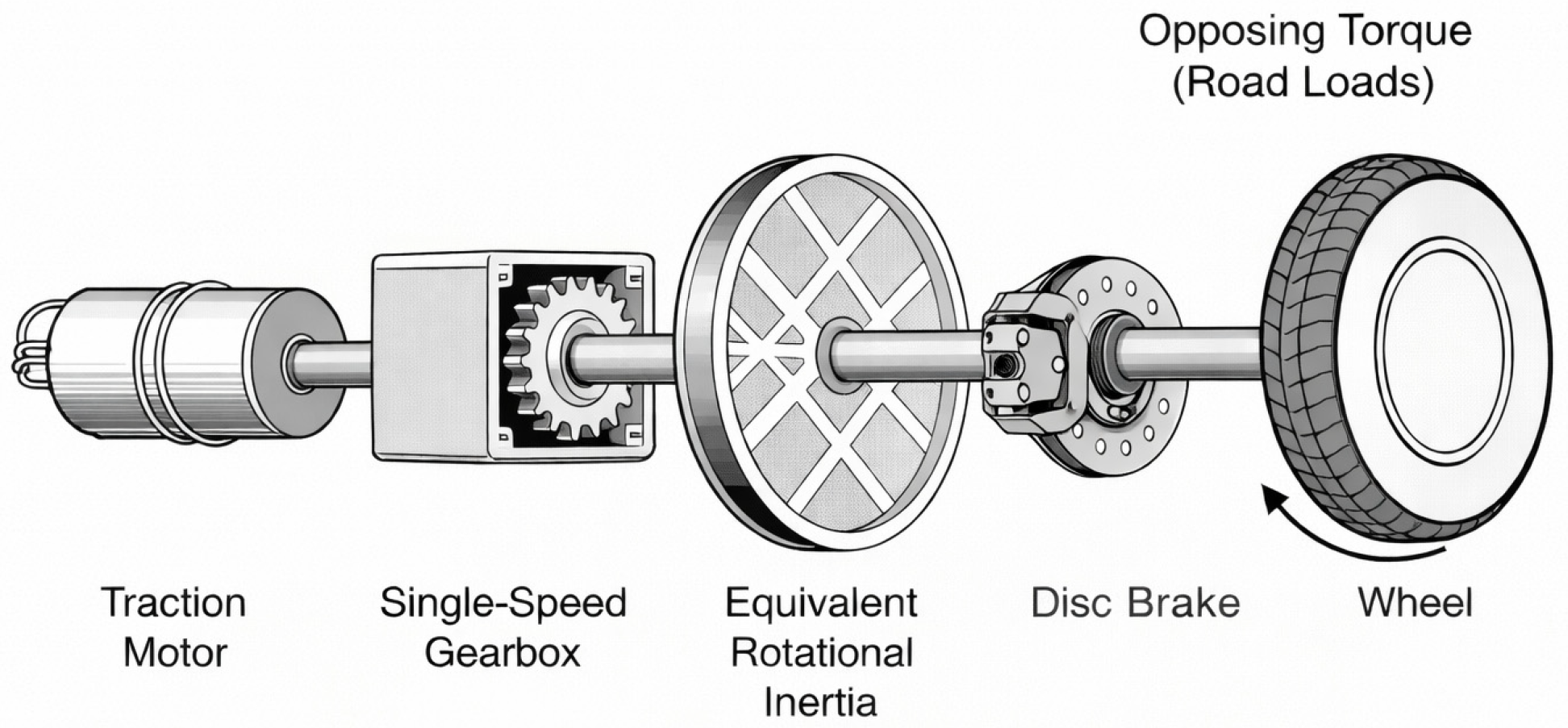
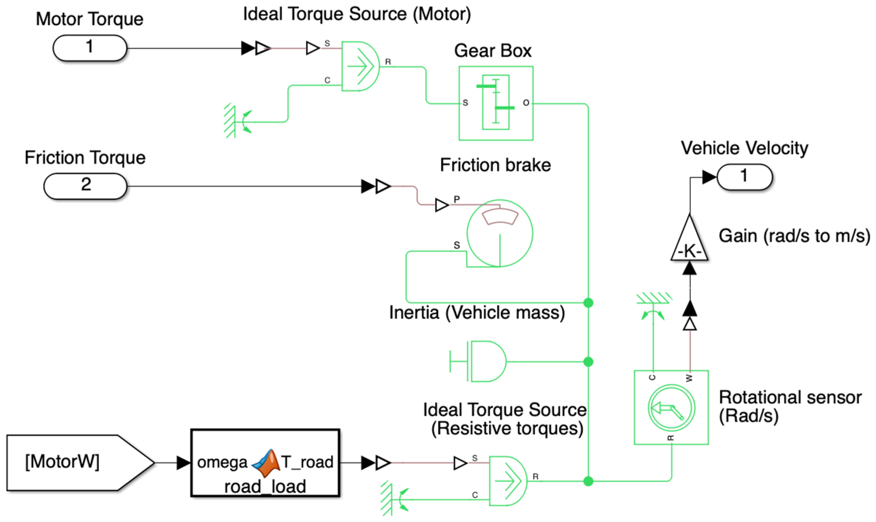
To satisfy these requirements with minimal structural complexity, the drivetrain is implemented as a traction motor driving a single-speed gearbox, which, in turn, drives an equivalent rotational inertia representing the vehicle mass. A friction brake acts on the same shaft, and the combined road loads are converted into an equivalent opposing torque at the wheel, as shown in Figure 1. This configuration provides a compact but physically meaningful basis for studying torque allocation, energy recovery, and battery loading in the subsequent control design and AI experiments.

3.2. BEV Drivetrain Modeling

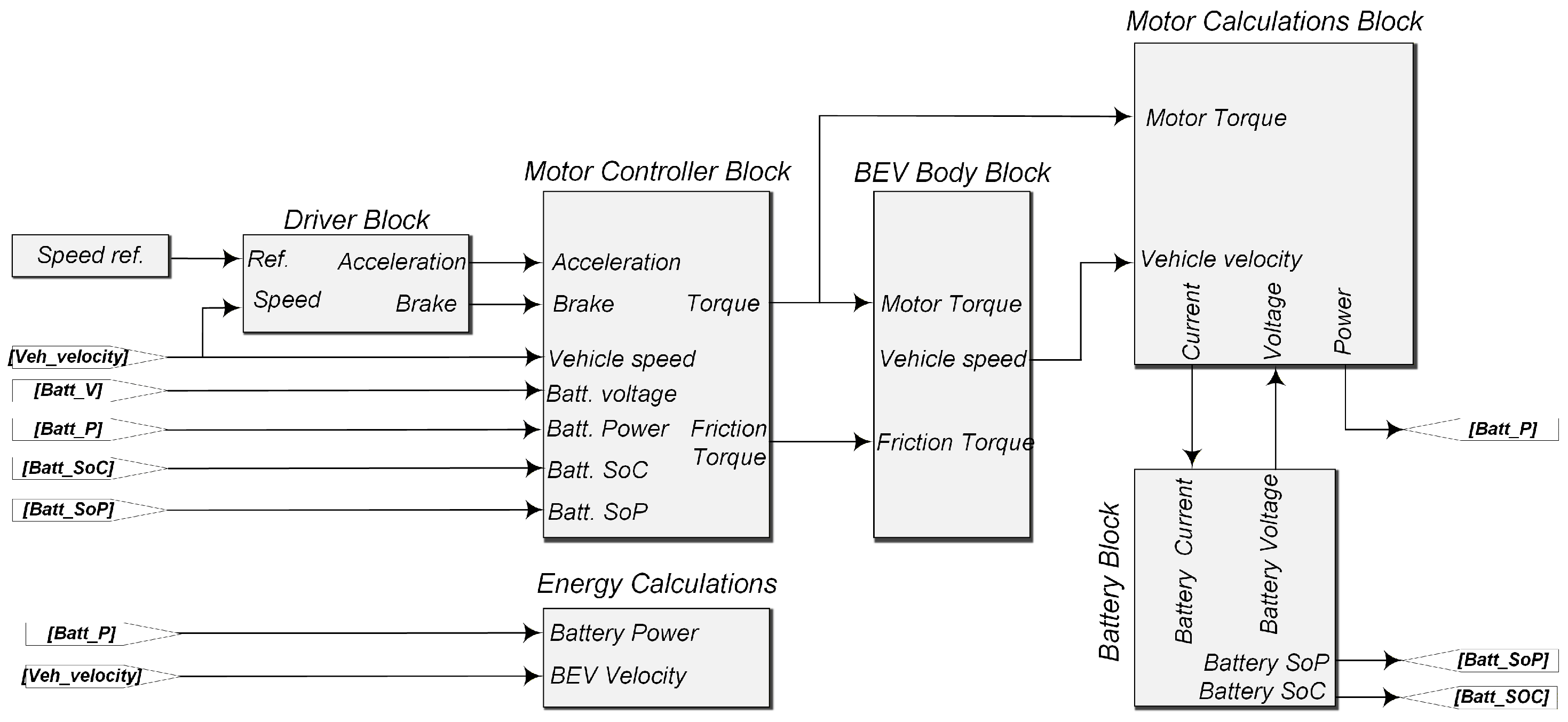
MATLAB/Simulink is used to establish the BEV drivetrain model and the related RBS control logics. MATLAB tools enable rapid prototyping and visualization of dynamic system interactions. A screenshot of the Simulink drivetrain model is shown in Figure 2.

3.2.1. Longitudinal Driver Model

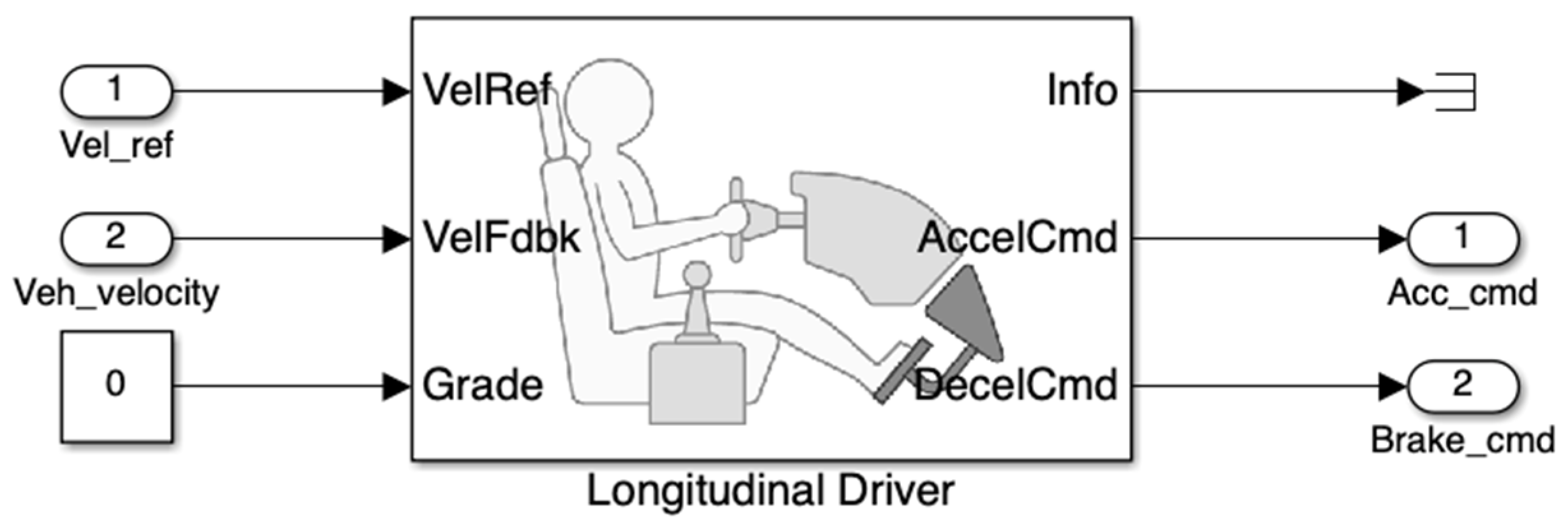
The driver employs the Longitudinal Driver block from Simulink to automate velocity tracking and emulate driver pedal inputs. The block utilizes a proportional–integral (PI) control strategy to generate normalized acceleration and braking commands based on the difference between a reference velocity $v_{ref}$ and the measured vehicle velocity v. Two input signals are required: the interpolated reference velocity and real-time vehicle velocity feedback. The resulting outputs are mapped to pedal commands for acceleration and braking.

Figure 3 shows the configuration and inputs/outputs of the driver block within the overall Simulink model. The PI controller logic implemented in the block is expressed as [30]:

$$y={\displaystyle \frac{K_{ff}}{v_{nom}}}{v}_{\mathrm{ref}}+{\displaystyle \frac{K_p{e}_{ref}}{v_{nom}}}+{\displaystyle \int \left(\frac{K_i{e}_{ref}}{v_{nom}}+K_{aw}{e}_{out}\right)}dt+K_g{y}^{\prime }$$

(5)

where $v_{nom}$ is the nominal vehicle speed, $K_p$ is the proportional gain, $K_i$ is the integral gain, $K_{aw}$ is the anti-windup term, $K_{ff}$ is the speed feedforward term, and $K_g$ is the grade angle feedforward gain. The error terms $e_{ref}$ and $e_{out}$ can be written as follows:

$$e_{ref}=v_{\mathrm{ref}}-v$$

(6)

$$e_{out}=y_{sat}-y$$

(7)

The output y is limited to the admissible range $[-1, 1]$ using:

$$y_{sat}=\left\{\begin{array}{ll}-1\hfill & y<-1\hfill \\ y\hfill & -1\le y\le 1\hfill \\ 1\hfill & y>1\hfill \end{array}\right.$$

(8)

Here, the output y is the longitudinal control command acting as a virtual pedal signal, which represents the driver’s intent (y > 0 represents acceleration while y < 0 represents braking/deceleration). Pedal command signals are then derived as follows:

$$y_{acc}=\left\{\begin{array}{ll}0\hfill & y_{sat}<0\hfill \\ y_{sat}\hfill & 0\le y_{sat}\le 1\hfill \\ 1\hfill & y_{sat}>1\hfill \end{array}\right.\hspace{1em}\hspace{1em}{y}_{dec}=\left\{\begin{array}{ll}0\hfill & y_{sat}>0\hfill \\ -y_{sat}\hfill & -1\le y_{sat}\le 0\hfill \\ 1\hfill & y_{sat}<-1\hfill \end{array}\right.$$

(9)

3.2.2. Electric Motor

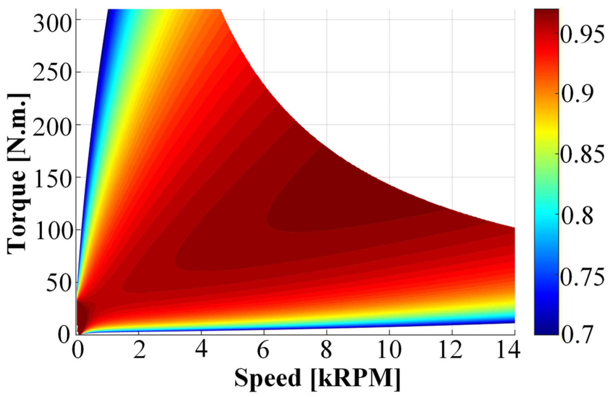
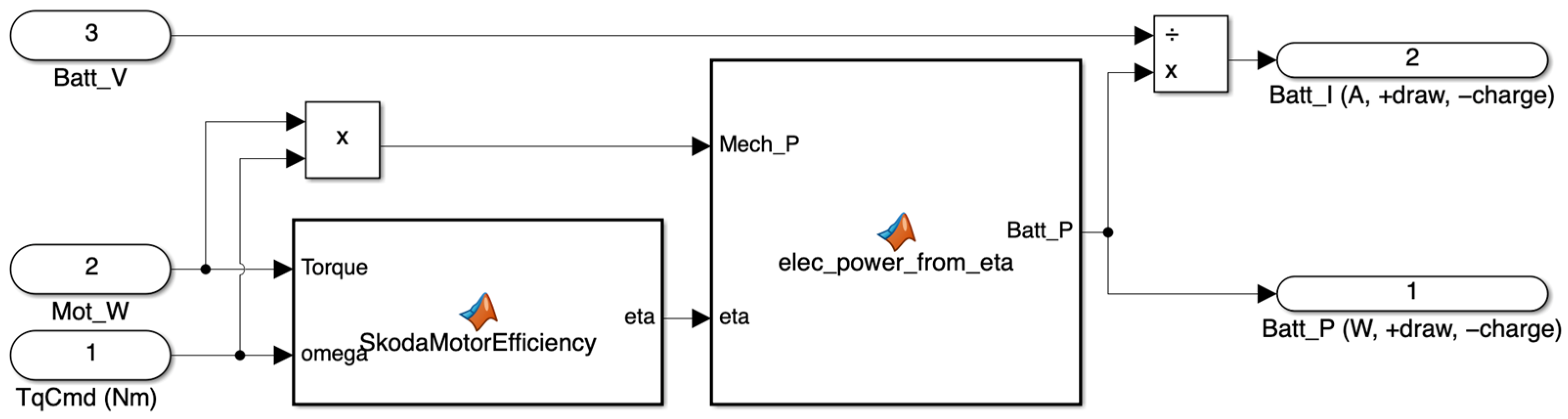
The electric motor is represented using an efficiency map and an Ideal Torque Source block, rather than a detailed physical model of a specific machine type. This efficiency map directly relates motor operating conditions (such as torque and speed) to efficiency values, enabling calculation of power losses and actual output without modeling the underlying electrical and magnetic processes. The primary motivation for this approach is to simplify the simulation while retaining accuracy in the assessment of energy flows and system performance. This is illustrated in Figure 4. The block receives the motor torque command $T_{qCmd}$ [Nm] (positive motoring, negative regeneration), motor rotational velocity ${\omega }_{mot}$ [rad/s], and battery terminal voltage $V_{batt}$ [V] and outputs the mechanical power at the shaft $P_{mech}$ [kW], power at the DC bus (positive draw, negative charge) $P_{DC}$ [W], battery current $I_{batt}$ [A], and instantaneous motor–inverter efficiency ${\eta }_{now}$ [-]. For a given operating point $({\omega }_{mot},T_{qCmd})$ the map implements the following:

$$P_{\mathrm{mech}} ={\omega }_{\mathrm{mot}}{T}_{\mathrm{qCmd}}$$

(10)

$$\eta =\eta ({\omega }_{\mathrm{mot}},T_{\mathrm{qCmd}})$$

(11)

$$P_{\mathrm{DC}}=\left\{\begin{array}{l}{\displaystyle \raisebox{1ex}{$P_{\mathrm{mech}}$}\!\left/ \!\raisebox{-1ex}{$\eta $}\right.}, P_{\mathrm{mech}}\ge 0\hspace{1em}\left(\mathrm{motoring}\right)\hfill \\ -\eta P_{\mathrm{mech}}, P_{\mathrm{mech}}<0\hspace{1em}\left(\mathrm{regeneration}\right)\hfill \end{array}\right.$$

(12)

$$I_{\mathrm{batt}}={\displaystyle \raisebox{1ex}{$P_{\mathrm{DC}}$}\!\left/ \!\raisebox{-1ex}{$V_{\mathrm{batt}}$}\right.}$$

(13)

The sign convention is such that $P_{DC}<0$ and $I_{batt}<0$ during regenerative braking (charging). The efficiency map is implemented as follows:

$$\eta =f({\omega }_{\mathrm{mot}},T_{\mathrm{qCmd}})$$

(14)

where at each point $\left({\omega }_{mot},T_{qCmd}\right),$ a scalar efficiency value $\eta$ is computed.

3.2.3. Motor Controller Model

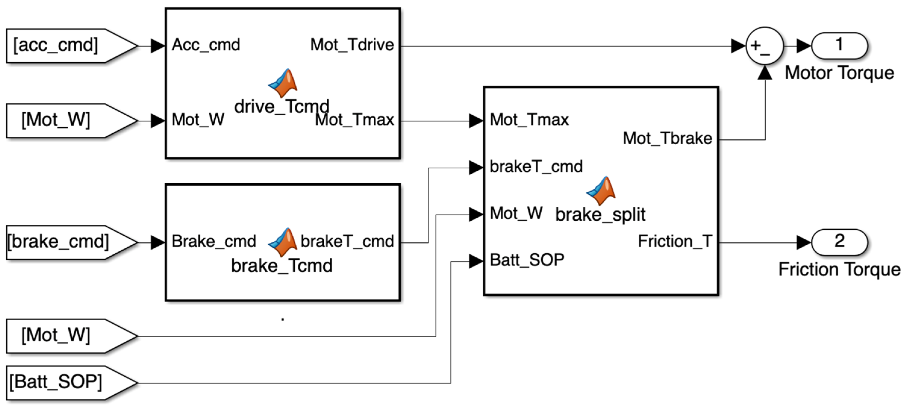
The motor controller subsystem translates accelerator and brake pedal inputs into appropriate drive and brake torque commands. For motoring, the controller computes the available torque envelope based on motor speed and power limits, applying a smooth taper to avoid abrupt transitions. For braking, the controller determines the torque split between regenerative and friction braking, taking into account speed-dependent fade, brake intensity, and battery power constraints. The computed torque commands are then fed directly into the efficiency map, which calculates the corresponding electrical power for accurate energy accounting. Additionally, these torque signals are input to the Ideal Torque Source, representing the electric motor in the drivetrain model by translating mechanical torque commands into motion. The implemented block diagram is illustrated in Figure 5.

The accelerator input, acc_cmd, is a normalized value in [0, 1] representing throttle demand. This input is scaled to compute the motoring torque envelope T_max as follows:

$$T_{\max }=\min (T_{maxmot},{\displaystyle \frac{P_{maxmot}}{w_{\mathrm{mot}}}})$$

(15)

where T_maxmot is the motor’s peak allowed torque, P_maxmot is the peak power output, and w_mot is the current motor speed (rad/s). To avoid an abrupt torque cutoff at the no-load speed, the maximum motoring torque is multiplied by a smooth taper function. Let w_taper denote the speed at which the reduction starts and w_no the no-load speed. The taper factor is defined as follows:

$$\mathrm{taper}(w_{\mathrm{mot}})=\left\{\begin{array}{ll}1\hfill & \left|w_{\mathrm{mot}}\right|<w_{\mathrm{taper}}\hfill \\ {\displaystyle \frac{1}{2}}\left(1+\cos \left({\displaystyle \frac{\pi \left(\left|w_{\mathrm{mot}}\right|-w_{\mathrm{taper}}\right)}{w_{\mathrm{no}}-w_{\mathrm{taper}}}}\right)\right)\hfill & w_{\mathrm{taper}}\le \left|w_{\mathrm{mot}}\right|<w_{\mathrm{no}}\hfill \\ 0\hfill & \left|w_{\mathrm{mot}}\right|\ge w_{\mathrm{no}}\hfill \end{array}\right.$$

(16)

The middle branch of (16) is constructed as a standard raised–cosine (cosine-taper) window, chosen to obtain a smooth transition between 1 and 0. First, the motor speed is normalized to:

$$z={\displaystyle \frac{\left|w_{\mathrm{mot}}\right|-w_{\mathrm{taper}}}{w_{\mathrm{no}}-w_{\mathrm{taper}}}}$$

(17)

so that $z=0$ at the onset of tapering $\left|w_{mot}\right|=w_{taper}$ and z = 1 at the no-load speed $\left|w_{mot}\right|=w_{no}$. Over this interval, the function $0.5\left(1+\mathrm{c}\mathrm{o}\mathrm{s}\left(\pi z\right)\right)$ decreases smoothly from 1 (at z = 0) to 0 (at z = 1), with zero slope at both endpoints. Substituting the expression for z into this cosine expression yields the middle case in (16). The effective maximum motoring torque envelope then becomes:

$$T_{\max }(w_{\mathrm{mot}})=T_{\max }(w_{\mathrm{mot}})\cdot \mathrm{taper}(w_{\mathrm{mot}})$$

(18)

so that the available torque is constant up to $w_{taper}$, smoothly decreases to zero between $w_{taper}$ and $w_{no}$, and is zero beyond the no-load speed. The actual motoring torque request sent to the drivetrain is then:

$$T_{\mathrm{drive\_cmd}}=\mathrm{acc\_cmd}\cdot T_{\max }(w_{\mathrm{mot}})$$

(19)

The brake pedal input brk_cmd is a normalized signal in the range [0, 1], where 0 corresponds to no braking and 1 to a full-brake request. The total commanded brake torque is:

$$T_{\mathrm{br},\mathrm{cmd}}=\mathit{brk\_cmd}\cdot T_{\mathrm{br},\max }$$

(20)

with T_br,max denoting the maximum available braking torque of the vehicle. This commanded torque is distributed between regenerative torque T_r and friction torque T_f with a speed-dependent fade of regeneration, meaning that the regenerative braking is progressively reduced as motor speed decreases. To model this effect, a scalar fade factor is defined as follows:

$$\mathrm{fade}(w)=\left\{\begin{array}{ll}0\hfill & w\le w_{\mathrm{off}}\hfill \\ {\displaystyle \frac{w-w_{\mathrm{off}}}{w_{\mathrm{full}}-w_{\mathrm{off}}}}\hfill & w_{\mathrm{off}}<w<w_{\mathrm{full}}\hfill \\ 1\hfill & w\ge w_{\mathrm{full}}\hfill \end{array}\right.$$

(21)

so that regeneration is disabled at low speed, increases linearly between w_off and w_full, and reaches full strength above w_full. The brake command determines the nominal share of the requested torque that may be provided, regeneratively:

$$\mathrm{share}(\mathit{brk\_cmd})=\left\{\begin{array}{ll}1\hfill & \mathit{brk\_cmd}\le 0.5\hfill \\ {\displaystyle \frac{0.8-\mathit{brk\_cmd}}{0.3}}\hfill & 0.5<\mathit{brk\_cmd}\le 0.8\hfill \\ 0\hfill & \mathit{brk\_cmd}>0.8\hfill \end{array}\right.$$

(22)

For light braking (brk_cmd $\le$ 0.5), the request is fully assigned to regeneration. Between 0.5 and 0.8, the regenerative share decreases linearly, and for hard braking (brk_cmd $>$ 0.8), the friction brakes are assumed to provide the entire additional torque. The maximum admissible regenerative torque is limited by the battery charging power and motor speed.

$$T_{r,\mathrm{cap},\mathrm{pow}}={\displaystyle \frac{P_{\mathrm{cap}}}{\eta w}}$$

(23)

where P_cap is the battery-side charging power limit and $\eta$ is the regenerative efficiency. The overall regenerative torque cap is as follows:

$$T_{r,\mathrm{cap}}=\mathrm{fade}(w)\min (T_{\max },T_{r,\mathrm{cap},\mathrm{pow}})$$

(24)

The commanded regenerative and friction torques then become as follows:

$$T_r=\mathrm{share}(\mathit{brk\_cmd})\min (T_{\mathrm{br},\mathrm{cmd}},T_{r,\mathrm{cap}}),\hspace{1em}\hspace{1em}{T}_f=T_{\mathrm{br},\mathrm{cmd}}-T_r$$

(25)

3.2.4. BEV Body Model

The vehicle body and drivetrain are modeled as a single-speed, two-wheel-drive electric powertrain: a BEV motor drives an inertial disk (representing the car mass) through a gearbox. This subsection details the modeling of the inertial load, frictional brakes, gearbox, and resistive torques that together define the dynamics of the vehicle. This implementation, illustrated in Figure 6, is described in detail below. In the implemented model, only a single axle is represented, and the load transfer between the rear and front axles is neglected. This simplification is intentionally performed to reduce model complexity related to brake force proportioning, ABS coordination, etc. Accordingly, the full vehicle mass and all longitudinal road loads are mapped to an equivalent single wheel. This preserves the correct longitudinal dynamics while enabling focused analysis of energy flow, torque blending, and control strategies. The total vehicle inertia is represented using the Inertia block from Simulink. The equivalent rotary inertia applied at the wheel shaft is computed as follows:

$$J_{\mathrm{Vehicle}}=M_{\mathrm{Vehicle}}\cdot R_{\mathrm{Wheel}}^2$$

(26)

where M_Vehicle is the vehicle mass, and R_Wheel is the effective wheel radius. The brake system is modeled using the Disc Brake block from Simulink. A normalized brake command $\mathit{brk\_cmd}\in [0,1]$ is scaled to a hydraulic pressure P (in Bars), calibrated such that $\mathit{brk\_cmd}=1$ corresponds to a severe braking or full-stop event. Internally, the block computes the friction torque based on the applied pressure P, the actuator bore diameter D_b, the mean pad radius R_m, the number of pads N, and the kinetic friction coefficient ${\mu }_k$. For a rotating wheel ($\omega \ne 0$), the maximum brake torque is as follows:

$$T={\displaystyle \frac{{\mu }_{k}P\pi D_b^2{R}_{m}N}{4}}$$

(27)

A fixed-ratio single-speed gearbox is represented using the Gearbox block from Simulink. The gearbox connects the motor to the wheel and transmits speed and torque between them. Gearbox efficiency is neglected for simplicity. The core mechanical relationship is as follows:

$$G={\displaystyle \frac{{\omega }_m}{{\omega }_w}}={\displaystyle \frac{T_w}{T_m}}$$

(28)

where ${\omega }_m\left(T_m\right)$ and ${\omega }_w\left(T_w\right)$ are the angular velocity (torque) of the motor and wheel, respectively. All external road loads, i.e., aerodynamic drag, rolling resistance, viscous friction, and grade resistance, are combined into a single resistive torque. These are computed within the MATLAB Function block and summed into the drive shaft via an Ideal Torque Source block. The vehicle velocity V and wheel angular velocity ${\omega }_w$ are related as follows:

$$V={\omega }_w\cdot R_{\mathrm{Wheel}}$$

(29)

The resistive components are calculated as follows. The Aerodynamic drag force is calculated as:

$$T_d={\displaystyle \frac{1}{2}}\rho C_{d}A{R}_{\mathrm{Wheel}}{V}^2$$

(30)

where $\rho$ is air density [kg/m³], C_d is the drag coefficient, A is frontal area [m²], R_Wheel is the wheel radius, and V is vehicle velocity [m/s]. The rolling resistance force is calculated as:

$$T_{rr}=C_{rr}{M}_{\mathrm{Vehicle}}g{R}_{\mathrm{Wheel}}\cos (\theta )$$

(31)

where C_rr is the rolling resistance coefficient, g is the gravitational acceleration, and $\theta ={tan}^{-1}\left(grade\left[\%\right]/100\right)$ converts percentage grade to radians. A positive $\theta$ models uphill, while negative $\theta$ models downhill. The viscous friction force is calculated using the following formula:

$$T_v=b_{\mathrm{vis}}V$$

(32)

where b_vis is a viscous damping constant. Finally, the force associated with the road slope (grading) is obtained as follows:

$$T_g=M_{\mathrm{Vehicle}}g{R}_{\mathrm{Wheel}}\sin (\theta )$$

(33)

The total reactive torque can then be obtained by summing all the resistive forces as follows:

$$T_{\mathrm{road}}=-(T_{rr}+T_g+T_d+T_v)$$

(34)

The negative sign indicates opposition to vehicle movement. For numerical stability near zero speed, a smoothed sign function based on the hyperbolic tangent is used:

$$\mathrm{sgn}(\omega )=\tanh \left({\displaystyle \frac{\omega }{{\omega }_0}}\right)$$

(35)

This suppresses chattering and ensures a smooth, continuous transition from standstill to motion.

3.2.5. Battery Model

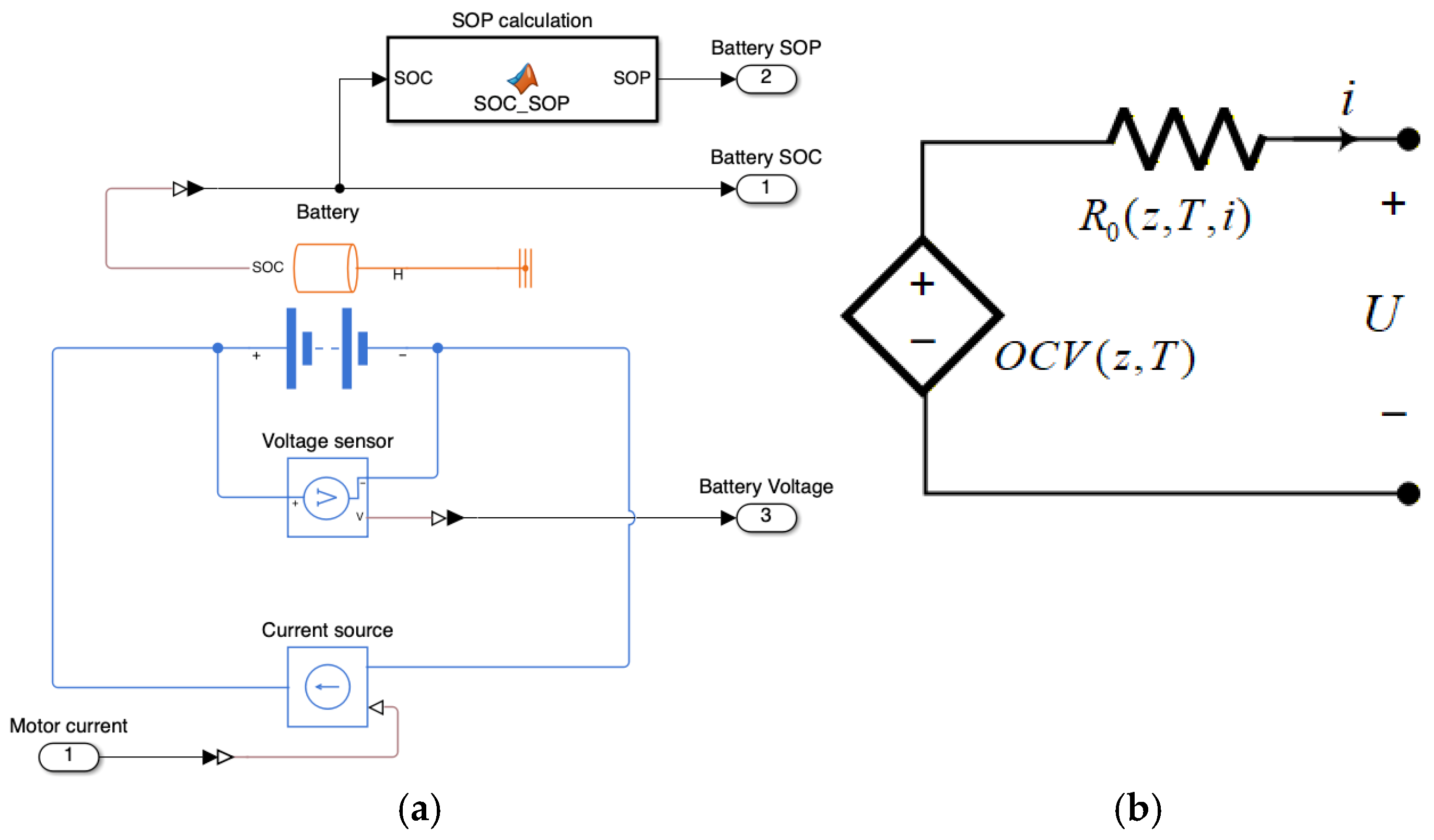
The Battery (Table-Based) block from MATLAB’s Simscape Electrical is used to model the battery. The block implements an equivalent circuit model (ECM) whose parameters are obtained from tabulated data. In particular, the block uses lookup tables to describe the open-circuit voltage (OCV), internal resistance, and optional dynamic resistive–capacitance (RC) elements as functions of SoC, cell temperature, and current direction. Figure 7a shows the battery subsystem implemented in Simulink, as well as the ECM used for battery modeling, in which R₀ denotes the battery internal resistance, OCV denotes the internal open-circuit voltage, i is the battery current (i > 0 during discharging and i < 0 during charging), and U is the terminal voltage. From Figure 7b, one can write:

$$U=\mathrm{OCV}(z,T)-R_0(z,T,i)\times i$$

(36)

where z is the SoC, and T is the temperature. With the OCV and internal resistance R₀ obtained from user-supplied lookup tables. The OCV curve is based on a representative NMC cell discharge characteristic typical of high-energy automotive cells [31]. The per-cell OCV values used in this work are as follows:

$$\begin{array}{l}\hspace{0.17em}\hspace{0.17em}\hspace{0.17em}\hspace{0.17em}\hspace{0.17em}\hspace{0.17em}\hspace{0.17em}\hspace{0.17em}\hspace{0.17em}\hspace{0.17em}\hspace{0.17em}\hspace{0.17em}\hspace{0.17em}\hspace{0.17em}\hspace{0.17em}\hspace{0.17em}\hspace{0.17em}\hspace{0.17em}\hspace{0.17em}\hspace{0.17em}\hspace{0.17em}\hspace{0.17em}z\in [0.0,\hspace{0.33em}0.1,\hspace{0.33em}0.2,\hspace{0.33em}0.3,\hspace{0.33em}0.4,\hspace{0.33em}0.5,\hspace{0.33em}0.6,\hspace{0.33em}0.7,\hspace{0.33em}0.8,\hspace{0.33em}0.9,\hspace{0.33em}1.0]\\ {\mathrm{OCV}}_{\mathrm{cell}}(z)=[3.34,\hspace{0.33em}3.53,\hspace{0.33em}3.59,\hspace{0.33em}3.63,\hspace{0.33em}3.66,\hspace{0.33em}3.70,\hspace{0.33em}3.75,\hspace{0.33em}3.83,\hspace{0.33em}3.92,\hspace{0.33em}4.03,\hspace{0.33em}4.13]\end{array}$$

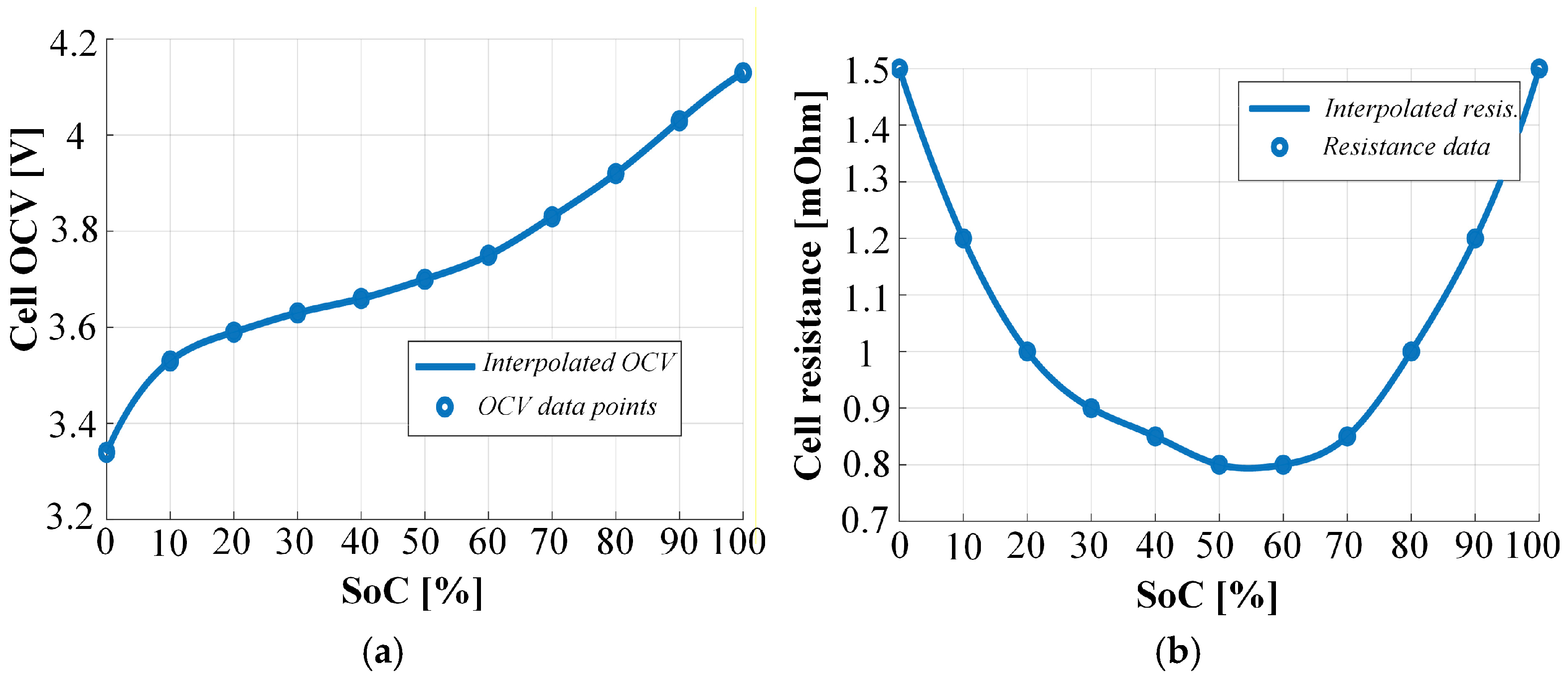
The OCV curve is shown in Figure 8a. To obtain pack-level voltages for the 96s3p configuration, the OCV table is scaled by the following series cell count:

$${\mathrm{OCV}}_{\mathrm{pack}}(z)=96\cdot {\mathrm{OCV}}_{\mathrm{cell}}(z)$$

(37)

This yields terminal voltages in the range [240, 403] V, consistent with public data for the Enyaq iV 80 battery pack. The internal resistance model follows the same SoC grid as the OCV table and reflects the typical U-shaped dependence of cell resistance on the SoC. The per-cell discharge resistance values are provided below and shown in Figure 8b.

$$R_{0,\mathrm{cell}}(z)=[1.50,\hspace{0.33em}1.20,\hspace{0.33em}1.00,\hspace{0.33em}0.90,\hspace{0.33em}0.85,\hspace{0.33em}0.80,\hspace{0.33em}0.80,\hspace{0.33em}0.85,\hspace{0.33em}1.00,\hspace{0.33em}1.20,\hspace{0.33em}1.50] \mathrm{m}\mathrm{\Omega }$$

Because the pack consists of 96 series cells and three parallel strings, the pack-level resistance during discharge is calculated as follows:

$$R_{0,\mathrm{pack}}(z)={\displaystyle \raisebox{1ex}{$96\times R_{0,\mathrm{cell}}(z)$}\!\left/ \!\raisebox{-1ex}{$3$}\right.}$$

(38)

A similar approach yields internal resistance during the charging (regenerative braking) process. The SoP calculation is accordingly fulfilled using the method proposed in [31]. The SoP approach is used to calculate power limits by the model, while the RL controller is trained to learn these dynamic limits inherently into itself.

3.3. Reference BEV

The reference vehicle is considered to be the Skoda Enyaq iV 80 with a 150 kW drivetrain. The main vehicle and powertrain parameters used in the simulation model are summarized in

Table 1. Simulation parameters considered for the studied BEV.

Category/Parameter	Value/Unit
Powertrain
Motor type	Permanent Magnet Synchronous Motor (PMSM)
Maximum Power	150 kW
Maximum Torque	310 Nm
No-load speed	~14,000 rpm
Gearbox	Single-speed reduction ≈ 10.5:1 ratio
Battery System
Battery type	Lithium-ion (Nickel Manganese Cobalt Oxide)
Configuration	96s3p
Nominal voltage	352 V
Usable capacity	77 kWh
Performance
Top Speed	160 km/h
Acceleration (0–100 km/h)	8.7 s
Energy consumption (WLTP)	170 Wh/km
Stopping distance (130–0 km/h)	80 m
Vehicle body and aerodynamics
Drag coefficient (Cd)	0.255
Frontal area (A)	2.54 m2
Wheel radius (RWheel)	0.358 m
Kerb weight (MVehicle)	2148 kg

. It should be noted that some of the required model parameters (such as vehicle mass, battery capacity, and rated motor power) are taken directly from manufacturers and database specifications, while others (such as drivetrain efficiency and motor no-load speed) are estimated to match typical values reported in the literature and public data sources. As described in Section 3.2.4, the friction brake block is parameterized by the mean pad radius, cylinder bore, and number of brake pads. In the absence of detailed caliper data for the reference vehicle, these parameters are selected to represent a typical front-axle disk brake for a mid-size BEV, with mean pad radius r_pad = 0.14 m, cylinder bore diameter d_bore = 0.057 m, and two brake pads per caliper (N_pads = 2). The input to the Frictional Brake block is hydraulic pressure, whereas the high-level brake command in the vehicle model is a normalized signal in the range 0–1. To obtain a realistic mapping between this normalized command and the physical brake torque, a simple calibration procedure is applied. First, a target stopping distance from 130 km/h to 0 km/h is defined, consistent with representative high-performance braking data reported in [32] (≈80 m). The vehicle model is then driven to a steady speed of 130 km/h, and a full brake command (brk_cmd = 1) is applied. A scalar gain is inserted between the normalized brake signal and the brake pressure input, and this gain is tuned such that the simulated stopping distance matches the 80 m target. In the final model, a gain of 180 yields a stopping distance of $\approx$80 m, and the resulting brake torque is $\approx$4400 Nm. This calibration effectively defines the maximum friction brake torque available in the simulation. It is further assumed that any higher equivalent braking torque demand would lead to wheel slip and thus lie outside the admissible operating region of the tire-road interface.

As for the electric motor efficiency map, exact data for the Skoda Enyaq iV 80 drive motor is unavailable. To circumvent this, a general polynomial efficiency mapping approach is adopted following the method proposed in [21]. This method is physically grounded and widely used for practical electric machine modeling when detailed test data is unavailable. The loss function model is based on the observation that the power loss P_loss in an electrical machine can be described as a sum of terms, each involving integer powers of torque (T) and speed ($\omega$), as originally proposed in [21]:

$$P_{loss}(T,\omega )={\displaystyle \sum _{m,n}{k}_{mn}}{T}^m{\omega }^n$$

(39)

where k_mn are fitting coefficients for each term, and m and n are integers. This polynomial approach has a solid physical basis. In a typical PMSM, the no-load iron (eddy-current) losses are proportional to ${\omega }^2$, copper losses are proportional to T² (torque is proportional to current), and cross-terms and higher-order effects (windage, field-weakening) may be neglected. Thus, for first-order loss estimation, one can obtain a simple approximation as follows:

$$P_{loss}(T,\omega )=k_{20}{T}^2+k_{02}{\omega }^2$$

(40)

The efficiency map in this work is constructed by synthesizing a polynomial loss model in per-unit (p.u.) coordinates, scaled to the Skoda motor’s rated values:

$$T_{\mathrm{pu}}={\displaystyle \frac{T}{T_b}},\hspace{1em}{\omega }_{\mathrm{pu}}={\displaystyle \frac{\omega }{{\omega }_b}}$$

(41)

where T_b = 310 Nm and ${\omega }_b$ = 2$\pi \times {\displaystyle \frac{\mathrm{14,000}}{60}}\mathrm{r}\mathrm{a}\mathrm{d}/\mathrm{s}$(motor peak specifications). Using the polynomial form proposed in [21], a custom set of coefficients is synthesized in this work to emulate the loss behavior of the traction motor:

$$\begin{array}{l}{P}_{\mathrm{loss},\mathrm{pu}}=-0.002+0.175{\omega }_{\mathrm{pu}}-0.065T_{\mathrm{pu}}+0.181{\omega }_{\mathrm{pu}}^2+0.577T_{\mathrm{pu}}{\omega }_{\mathrm{pu}} +\\ \hspace{0.17em}\hspace{0.17em}0.697T_{\mathrm{pu}}^2+0.443{\omega }_{\mathrm{pu}}^3-0.542T_{\mathrm{pu}}^2{\omega }_{\mathrm{pu}}-1.043T_{\mathrm{pu}}{\omega }_{\mathrm{pu}}^2+0.942T_{\mathrm{pu}}^3\end{array}$$

(42)

The actual machine loss in watts is obtained by scaling the per-unit loss with a loss base power:

$$P_{\mathrm{loss}}=P_{\mathrm{loss},\mathrm{pu}}\cdot P_{\mathrm{loss},\mathrm{base}}$$

(43)

In this work, P_loss,base is set at 9 kW. This value is chosen to be consistent with typical loss levels reported for high-power BEV traction machines, where rated efficiencies in the range of 95–97% imply loss fractions of approximately 3–5% of the mechanical output power at high load [21]. For a 150 kW drive, this corresponds to a loss range of roughly 4.5–7.5 kW at high torque and speed. The instantaneous efficiency is then calculated using:

$$\eta (T_m,{\omega }_m)={\displaystyle \frac{P}{P+P_{\mathrm{loss}}}}$$

(44)

Figure 9 shows the resulting motor efficiency map across the expected operating range. It is approximated that the map is symmetrical between the first and fourth quadrants, yielding equal efficiency during motoring and regenerative modes. This prevents the model from becoming unnecessarily complicated.

3.4. Preliminary Model Validation

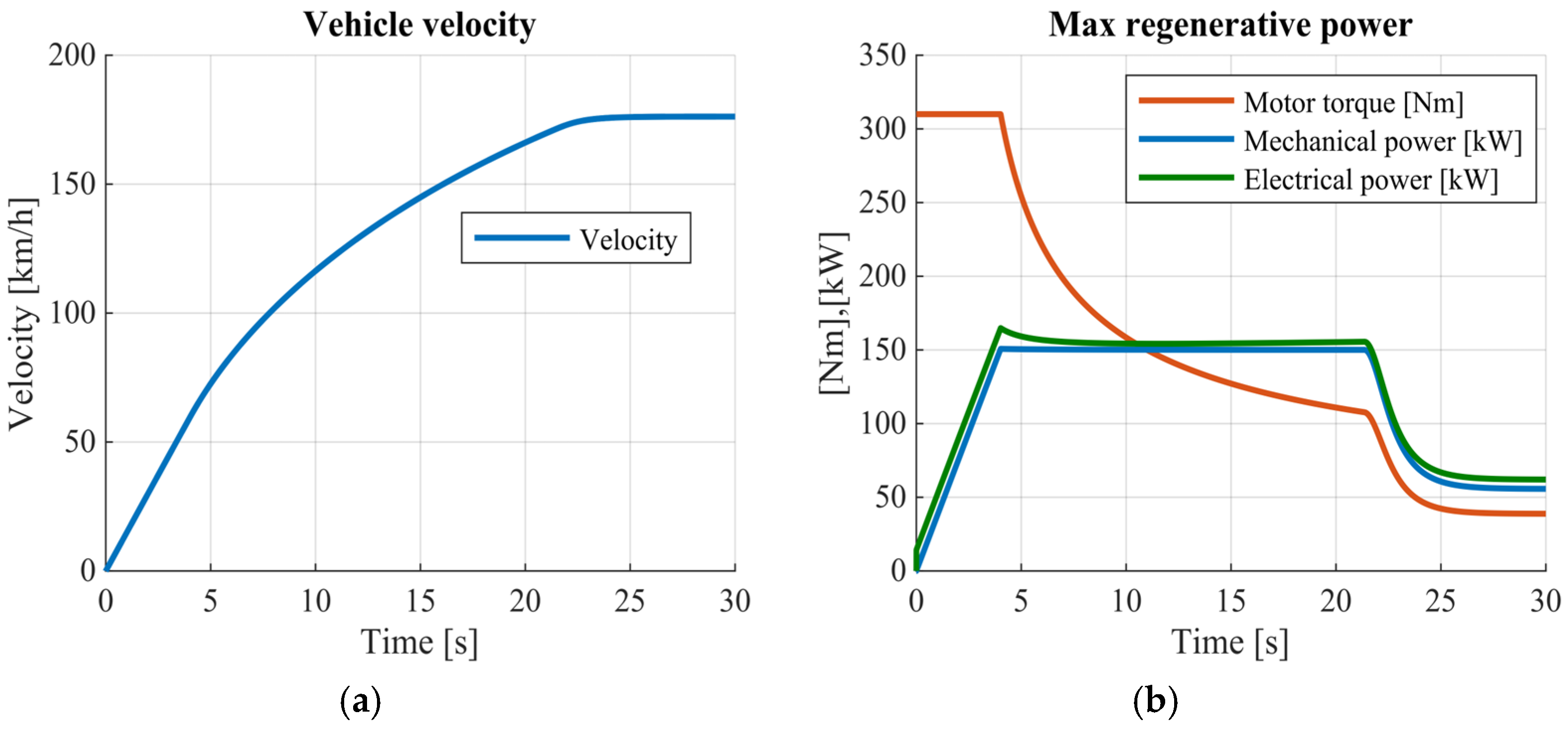
The Simulink model is preliminarily validated considering some performance criteria, including the 0–100 km/h acceleration time, achievable top speed, maximum motor torque, and energy consumption over a Worldwide Harmonized Light-Vehicles Test Procedure (WLTP) Class 3 drive cycle. A full-acceleration test is carried out by applying a constant accelerator command of 1.0, corresponding to a fully pressed pedal. The resulting vehicle speed and motor torque trajectories are shown in Figure 10.

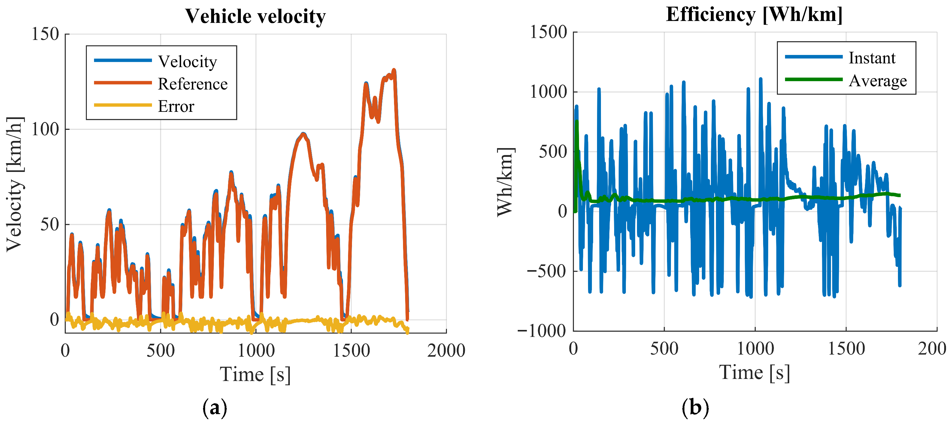
The simulated 0–100 km/h time is approximately 7.5 s, the steady-state top speed is about 176 km/h, and the peak motor torque is 310 Nm. Relative to the nominal Skoda Enyaq iV 80 specifications, this corresponds to deviations of roughly 11% in acceleration time, 9% in top speed, and negligible deviation in maximum torque. These differences are considered acceptable for the system-level analysis carried out in this work. To assess the overall energy efficiency, the model is driven over the WLTP Class 3 drive cycle for its full duration of approximately 30 min. The corresponding vehicle speed and specific energy consumption are shown in Figure 11.

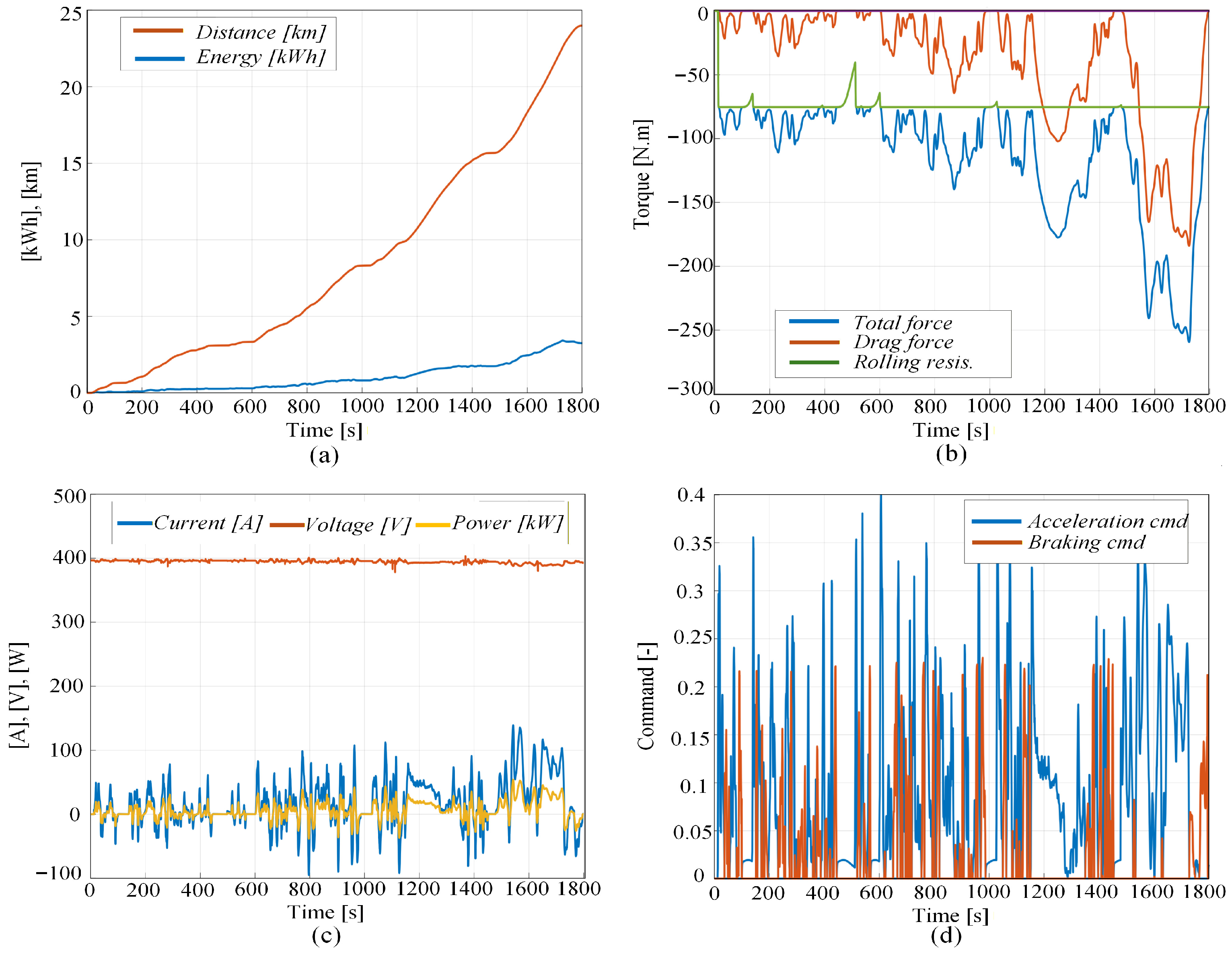
The simulated net energy consumption is 137 Wh/km. The difference with reference 159 Wh/km in part lies in simplifying modeling assumptions, such as standard air density (ambient temperature) and the omission of auxiliary loads/losses, which increase the measured consumption in a real car. Additional model simulation results are provided in Figure 12. Figure 12a shows the kWh energy consumption and total driven distance in a standard WLTP cycle. Figure 12b shows the simulated resistive forces during the WLTP cycle, in which the forces related to slope and viscosity are considered zero. The battery electrical measurements and the input commands are also, respectively, depicted in Figure 12c,d. These results confirm that the accelerating/braking commands/forces are correctly applied and meet the expectations from the established model.

In this paper, some parts of the model are deliberately simplified to improve the simulation speed and reduce training time over long-duration driving cycles. Such model simplifications are not expected to compromise the research conclusions because the proposed RL controller learns a constraint-aware policy structure rather than exploiting model-specific artifacts. Thus, absolute numerical results (e.g., percentage of recovered energy) may vary with the introduction of more model details, but the relative performance improvement and qualitative behavior of the RL-based strategy are expected to remain consistent.

The model is used in the next Section as a BEV digital twin to develop the proposed regenerative braking control strategy.

4. Principles of the Proposed Method

In this paper, an RL agent is trained and deployed in the RBS control system. RL learns a control policy by interacting with the environment, receiving a reward in response to actions [33]. RL is a perfect tool for sequential decision-making problems where current actions influence future states and rewards [34]. The RBS context demands a similar requirement, i.e., the controller must balance immediate energy recovery against future battery degradation, thermal constraints, and comfort. For instance, a gentle braking now may enable higher power regeneration in a subsequent phase (e.g., by keeping battery temperature optimal). The reward function in the RL can encode energy, comfort, and battery health simultaneously, enabling a multi-objective optimization of different control parameters. In the RL, an agent observes a state s_t, applies an action a_t, and receives a reward r_t from the environment. Over time, the agent learns a policy $\pi \left(a\right|s)$ that maximizes the expected long-term reward as follows:

$$J(\pi )={\mathbb{E}}_{\pi }\left[{\displaystyle \sum _{t=0}^{\infty }{\gamma }^t}{r}_t\right]={\mathbb{E}}_{\pi }\left[{\displaystyle \sum _{t=0}^{\infty }{\gamma }^t}r(s_t,a_t)\right]$$

(45)

where $s_t\in \mathcal{S}$ is the observation state at time t (battery SoC, vehicle speed, etc.), a_t$\in \mathcal{A}$ is the action at time t (regenerative motor torque command), $r_t=r\left(a_t,s_t\right)$ is the immediate reward obtained for action a_t in state $s_t$, $\gamma \in [0,1)$ is a discount factor influencing the weight for future rewards, $\pi \left(a\right|s)$ is the policy that prescribes which action a to take in state s, and ${\mathbb{E}}_{\pi }[·]$ is the expected value over trajectories generated by policy.

The RL agent will not replace the entire braking logic. Instead, it learns the decision layer that determines the regenerative torque share. Safety fallbacks (hydraulic braking, hard SoP limits, stopping distance constraints) remain active in the environment. The drivetrain model is simulated using MATLAB, and the model serves as a digital twin environment to train the RL agents using MATLAB’s Reinforcement Learning Toolbox. Additionally, a rule-based strategy is developed to serve as a baseline. The baseline controller follows the deterministic structure and logics described in Section 2, considering the feasible and edge operational boundaries, such as applicable maximum charging power levels that do not violate the control criteria. This enables a realistic assessment of the RL controller’s effectiveness in achieving the intended control objectives.

4.1. Architecture of the RL Agent

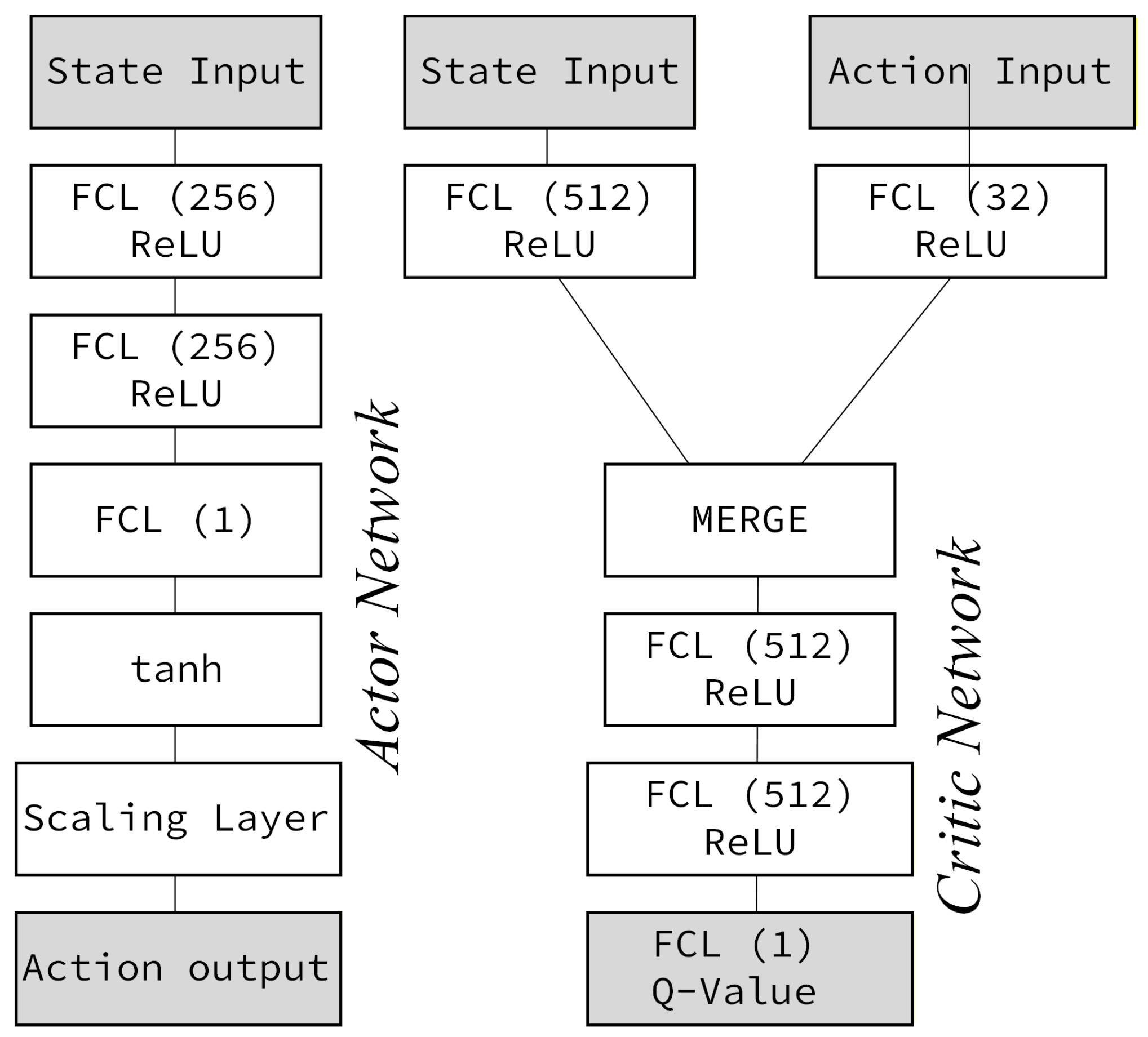
The RL agent is implemented as a DDPG controller consisting of an actor network (policy) and a critic network. DDPG was selected for two main reasons. First, it naturally accommodates continuous control actions, which are essential for the torque-split problem in the RBS. Second, it provides stable and smooth training behavior in deterministic environments, such as the digital twin simulation of the BEV considered in this study, where well-defined physical constraints (e.g., SoP limits) are present. In physical terms, the actor output represents the regenerative torque fraction used to split braking demand between the electric motor and friction brakes. The actor network maps the observation vector to a single continuous control action a_t. The actor features an input layer with dimensionality equal to the state vector, two fully connected layers (FCLs), and Rectified Linear Units (ReLUs) activation functions. Each of the FCLs contains 256 neurons. At the output, an FCL with one neuron is placed, followed by a hyperbolic tangent (tanh) activation function and a scaling layer. As for the critic, the network comprises two paths: a state stream with an FCL of 512 neurons followed by ReLU, and an action stream with a FCL of 32 neurons followed by ReLU. The two streams are then merged in order through an FCL (512 neurons), a ReLU function, an FCL (256 neurons), a ReLU function, and lastly an FCL (1 neuron). The architecture is selected following the choices commonly reported in the DDPG control tasks [33]. Figure 13 depicts the architecture of the actor and critical networks. Intuitively, the critic first builds an internal representation of the state (e.g., speed, SoC, braking demand) and a separate representation of the action (requested torque split). After merging these, the larger hidden layers allow the network to learn how state and action interact, including nonlinear effects such as the sharp change in value when the action approaches the SoP limit. The final layer is linear and outputs a single scalar value without any bounding.

In the DDPG agent, action a_t represents the regenerative torque fraction as follows:

$$T_{\mathrm{regen}}=a_t{T}_{\mathrm{req}},\hspace{1em}\hspace{1em}{T}_{\mathrm{fric}}=T_{\mathrm{req}}-T_{\mathrm{regen}}$$

(46)

4.2. Environment Design for RL Training

The nonlinear Simulink-based BEV drivetrain model developed in Section 3 serves as the environment for the RL training. The observation space is a six-dimensional state vector $o\in {\mathbb{R}}^6$, comprising the braking command (brake_cmd $\in [0,1]$), motor power P_ee (normalized to peak power), motor speed n_rpm (normalized to base speed), motor torque T_req (normalized to the peak torque), battery SoC, and SoP (P_cap). All components are scaled to [0,1] to improve learning stability. The normalization bases for speed and torque are considered as 4000 rpm and 300 Nm, respectively. The action space a_t is a single scalar representing the fraction of regenerative braking torque.

4.3. Reward Function Design

The reward function (RF) is designed to balance two objectives: (i) maximizing regenerative energy recovery under a time-varying SoP-based charging limit, and (ii) ensuring safe and smooth regenerative braking power levels. For the RF design, the following ratio is first defined and computed:

$$\chi ={\displaystyle \raisebox{1ex}{$P_{\mathrm{ee}}$}\!\left/ \!\raisebox{-1ex}{$P_{\mathrm{cap}}+\epsilon $}\right.}$$

(47)

where $\mathit{\epsilon }$ is a small number to avoid division by zero. This can be considered as a soft-constrained optimization problem, where the RL agent approximately solves to maximize P_ee (maximum recovery) while ensuring P_ee $\le$ P_cap (battery safety). The interpretation is as follows: (i) no regenerative power is used when $\chi =0$; (ii) the agent uses power up to the safe power cap of the battery when $\chi <1$; and (iii) when $\chi >1,$ the requested electric power exceeds the permissible battery power cap. Based on the definition, the reward is formulated considering the following three regions:

• Safe region (considered as $\chi \le 0.8$): The agent is far below the safety limit; thus, the regenerative energy term r_energy encourages regeneration by $r_{energy}=\chi$. This grows linearly from 0 to 0.8 and pushes the agent to increase regenerative power when it is clearly safe.
• Near the limit ($0.8<\chi \le 1$): The agent is close to the gap, so the reward rises more slowly: $r_{energy}=0.8+\phi (\chi -0.8)$, where $0<\phi <1$ balances between regeneration and safety, i.e., there is little gain in pushing right up to the exact limit.
• Over the cap ($\chi >1$): Exceeding the cap is discouraged by a penalty: $r_{energy}=-2(\chi -1)$. This enforces hard safety compliance by making constraint violation suboptimal. It ensures that the learned policy respects battery charging limits even without explicit hard constraints in the policy network.

Overall, this RF shaping teaches the agent to avoid wasting the regenerative potential while respecting the battery safety limit. To discourage very abrupt changes in the control action, a small smoothness penalty is added as $r_{smooth}=-0.05\times \left|a_{act}-a_{prev}\right|$, which encourages smoother braking. The weighting factor 0.05 is chosen to be small so that energy recovery dominates the learning objective while still nudging the agent towards less jerky commands. The final RF yields as follows:

$$r=r_{\mathrm{energy}}+r_{\mathrm{smooth}}$$

(48)

For numerical robustness, the RF is clipped to the interval [−2, 1] to prevent extremely large values from destabilizing training.

The reward parameters $\phi$, the penalty coefficient, and the smoothness weight are selected based on trial-and-error to reach satisfactory learning. The reward parameter is chosen to be 0.2. A higher $\phi$ enables a more aggressive use of the battery, while lowering it leads to more conservative behavior. Likewise, the penalty coefficient in r_energy determines the constraint strictness versus the learning speed, which is set to 2. The reward shaping in each region improves policy convergence. The linear region $\chi \le 0.8$ provides a consistent learning signal, accelerating early training. Near the constraint $\chi =1$, the reduced slope prevents oscillatory behavior and reduces variance in value estimation. Moreover, a strong penalty beyond $\chi >1$ discourages exploration in unsafe regions, improving stability in training. Finally, we emphasize that the RL policy operates within an environment where hard constraints (e.g., SoP limits, friction braking fallback) remain enforced at the system level. In addition, the RL agent is designed to only optimize the torque-split decision layer, not the full braking authority. This hierarchical design ensures that even if the rewards were imperfect, safety is not compromised.

4.4. Synthesizing the Training Data

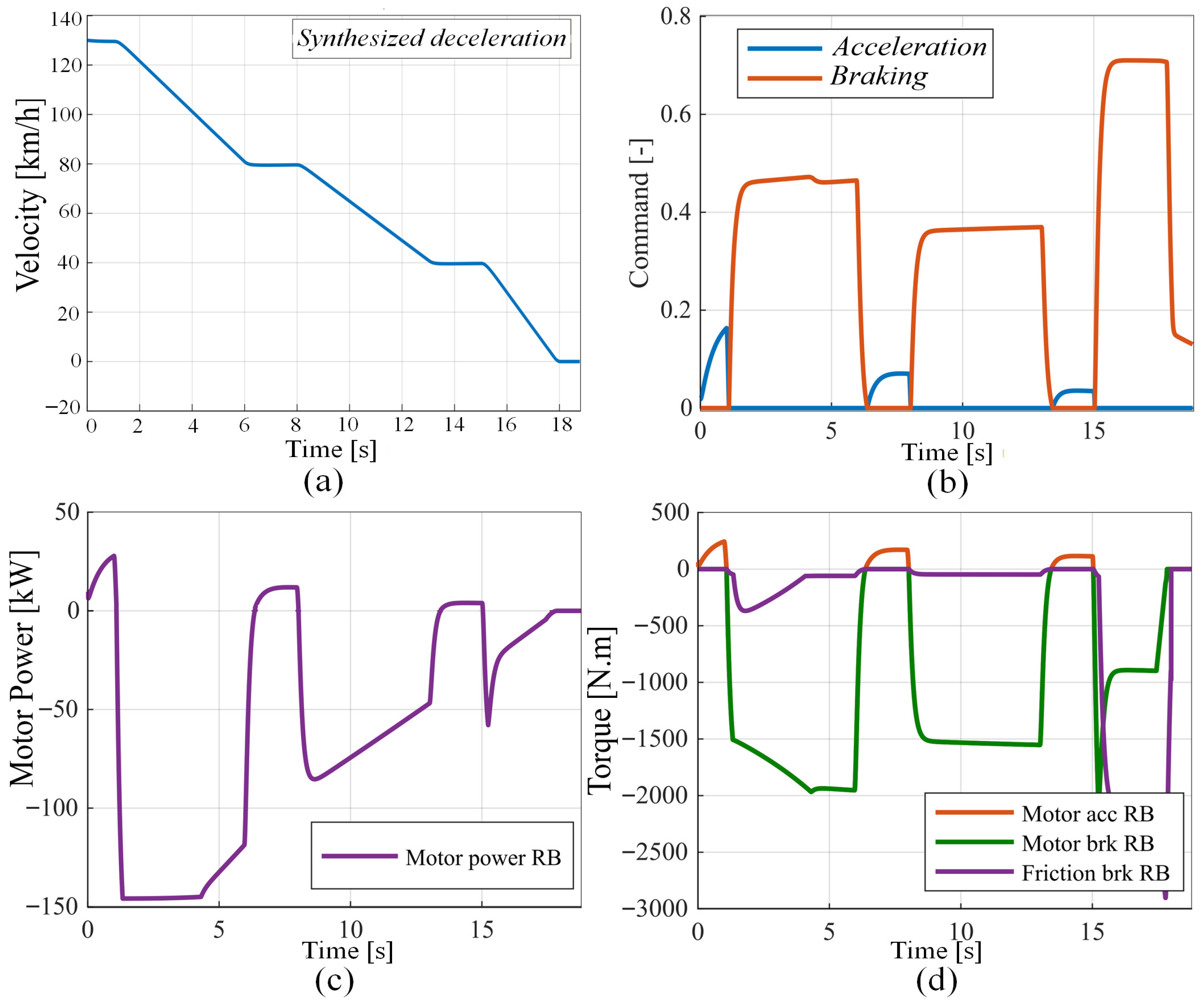
For the RL training, different braking scenarios are synthesized to emulate “soft braking”, “moderate braking”, and “hard braking”. The soft braking scenario involves pedal inputs below the blending threshold; thus, the braking is limited only by the requested deceleration and the motor’s regenerative capability. In moderate braking, the brake is considered strong enough to cap the regeneration by the 150 kW motor power limit, while the pedal input is still below the friction-blending threshold. As for the hard braking, the pedal input is considered above the blending threshold, so friction braking is added even if the power limit has not yet been reached. Three constant-deceleration phases are tuned to realize these cases, with target decelerations of $a_{soft}\approx -2.2 \mathrm{m}/{\mathrm{s}}^2$, $a_{med}\approx -2.8 \mathrm{m}/{\mathrm{s}}^2$, and $a_{hard}\approx -4.0 \mathrm{m}/{\mathrm{s}}^2$. In synthesized training episodes, medium braking is placed first because it reaches the regenerative power limit before the safety-related friction blending becomes active. Between each braking phase, the vehicle cruises for 2 s at constant speed. The total duration of the braking events is ~20 s. Figure 14 illustrates the BEV speed profile, the corresponding driver inputs, and axle torques. In Figure 14b, the first braking event is just below the blending threshold (brk_cmd = 0.5). Figure 14c shows that this still drives the motor up to the regenerative limit, after which additional torque is supplied by the friction brakes. In the last braking event, the pedal demand is well above the blending threshold, so the safety logic allocates a larger friction share, as seen in Figure 14d.

For each training episode, the initial battery SoC is sampled uniformly in the range 0.3–1. To consider the uncertainty in SoC estimation by the BMS, the SoC is randomly varied by $\pm 0.03$ during training. The RL agent then adjusts the brake bias over the three braking events to maximize the reward, i.e., to recover as much energy as possible while avoiding violations of the instantaneous SoP limit.

4.5. Training Procedure

Training is organized as a sequence of episodes, each corresponding to one complete simulation of a drive cycle. Within each episode, the following steps are repeated at every simulation time step: (i) The Simulink environment computes the current observations from the plant and driver signals and assembles the state vector s_t; (ii) The current reward r_t is computed, evaluating regenerative power utilization relative to the SoP-based power cap; (iii) The RL agent uses its current policy to select an action a_t, representing the regenerative braking fraction; (iv) The resulting transition $(s_t,a_t,r_t,s_{t+1})$ is stored in a replay buffer for off-policy learning, from which mini-batches are later sampled uniformly for gradient updates. The training hyperparameters are tabulated in

Table 2. RL’s training hyperparameters.

Parameter	Value
Sample time $∆t$	0.01 s
No. of episodes	5000
Actor learning rate ${\alpha }_{actor}$	$3\times {10}^{-4}$
Critic learning rate ${\alpha }_{critic}$	$3\times {10}^{-4}$
Replay buffer size	$2\times {10}^5$
Mini-batch size	256
Discount factor $\gamma$	0.995
Exploration noise type	Zero-mean Gaussian
Exploration noise variance	0.1
Network update rate $\tau$	0.001

. The hyperparameters were chosen considering typical values reported for neural networks in similar applications. The stochastic gradient descent algorithm is used to optimize networks during training. The training sessions were conducted on a laptop with specifications such as Apple Silicon M3 CPU and 18 GB of RAM using MATLAB version R2024a. The episodes required, on average, 5 s of wall-clock simulation time, resulting in a total training duration of approximately 6.94 h for the total number of episodes. 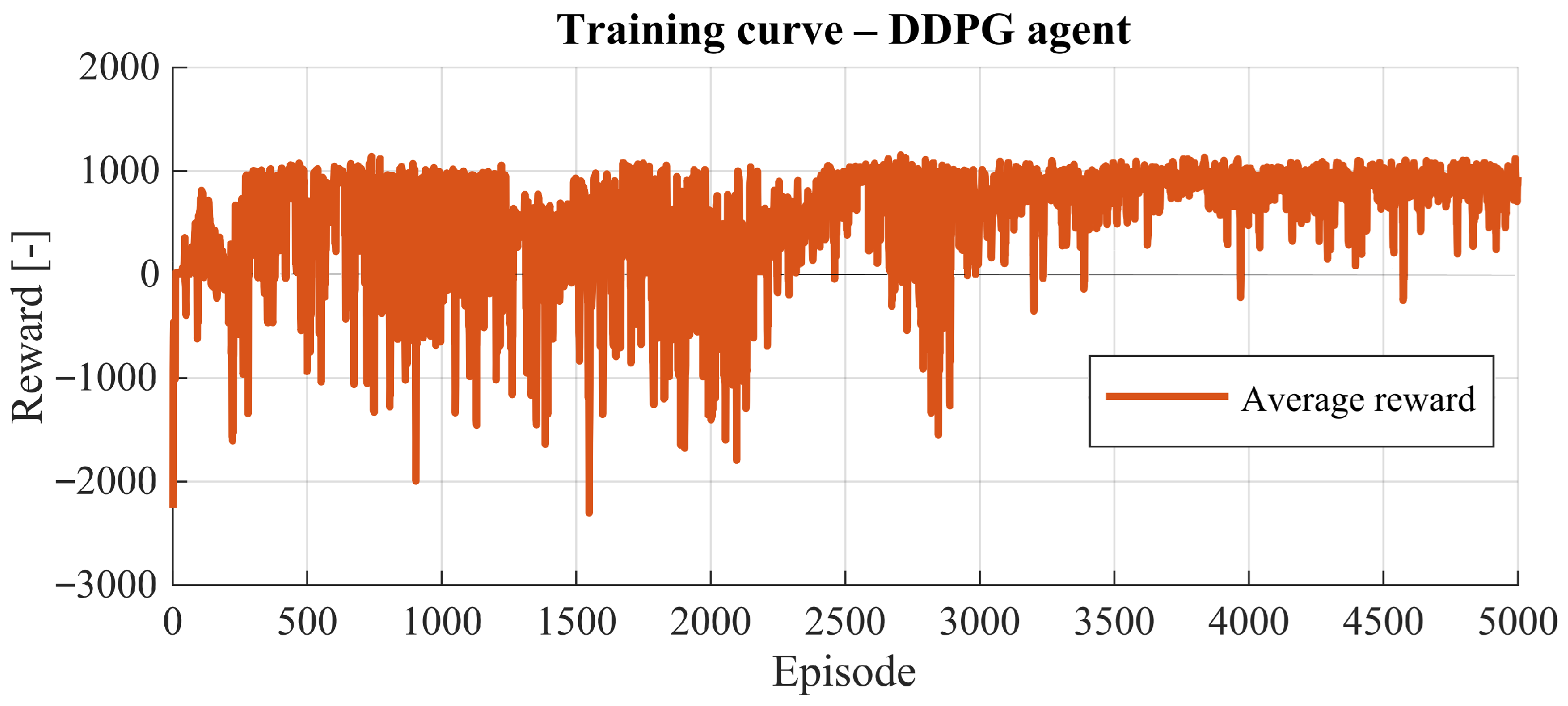Figure 15 shows the episodic reward over the training procedure. As seen, the running average increases over time while the frequency and severity of negative outliers gradually decrease as exploration noise decays, confirming a stabilizing policy.

5. Results and Discussions

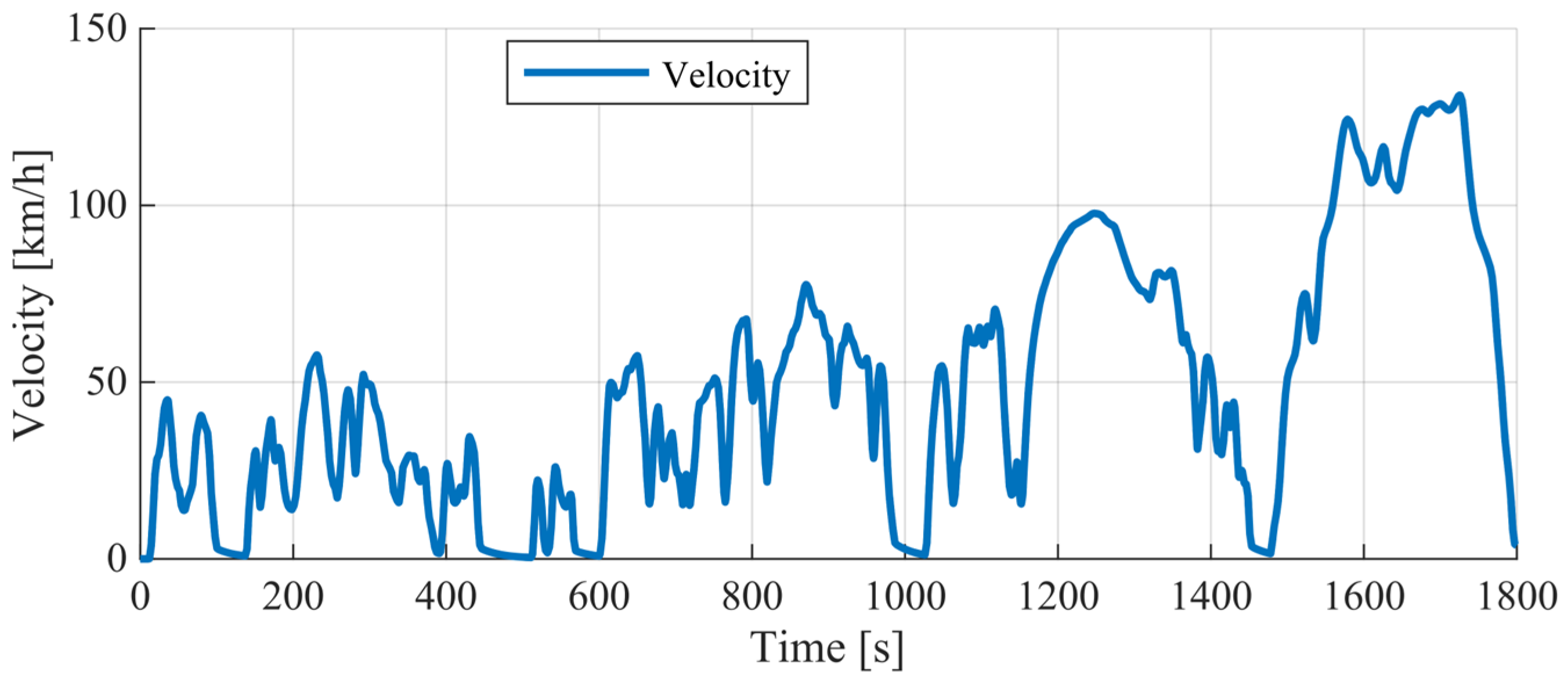
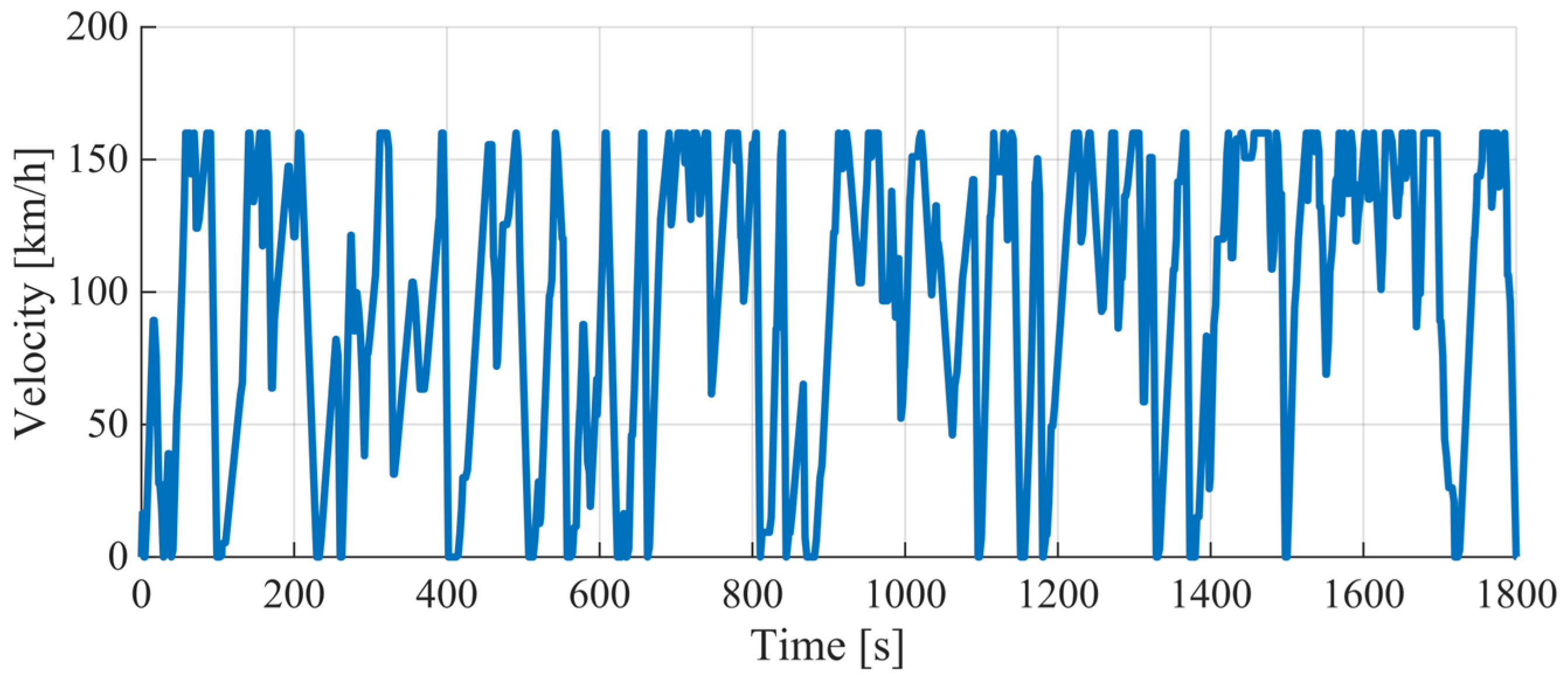
The proposed RL-based brake-split controller is evaluated using some performance criteria across multiple driving cycles that are different from the ones used during training. The tested cycles include both the standardized WLTP and a synthetic, randomness-rich driving profile containing numerous accelerations, soft and hard braking events, emergency stops, etc. The objective is to ensure not only standardized evaluation but also exposure of the RL controller to a wide spectrum of braking intensities that WLTP seldom provides. The driving cycles are shown in Figure 16 and Figure 17. The WLTP cycle is assessed in two configurations: (i) standard WLTP, which assumes a flat road; (ii) WLTP with a constant downhill gradient, corresponding to the same cycle executed on a uniform −5% road slope. To probe various battery operating regimes under power-limiting constraints, the validation is further conducted using different initial battery SoC levels: 0.75, 0.95, and 1. For each braking scenario, the regenerative braking power P_regen (instantaneous electrical power recovered to the battery), the SoC trajectory, and the specific energy consumption (Wh/km) are recorded. As a benchmark for evaluating the effectiveness of the proposed RL approach, an ideal controller is constructed as a “perfect” reference. This ideal controller always regenerates the maximum feasible amount of power permitted by the effective constraints and, therefore, by design, tracks P_max. By comparing the RL controller against this reference, it becomes possible to assess how closely the learned policy approaches ideal regenerative braking performance. 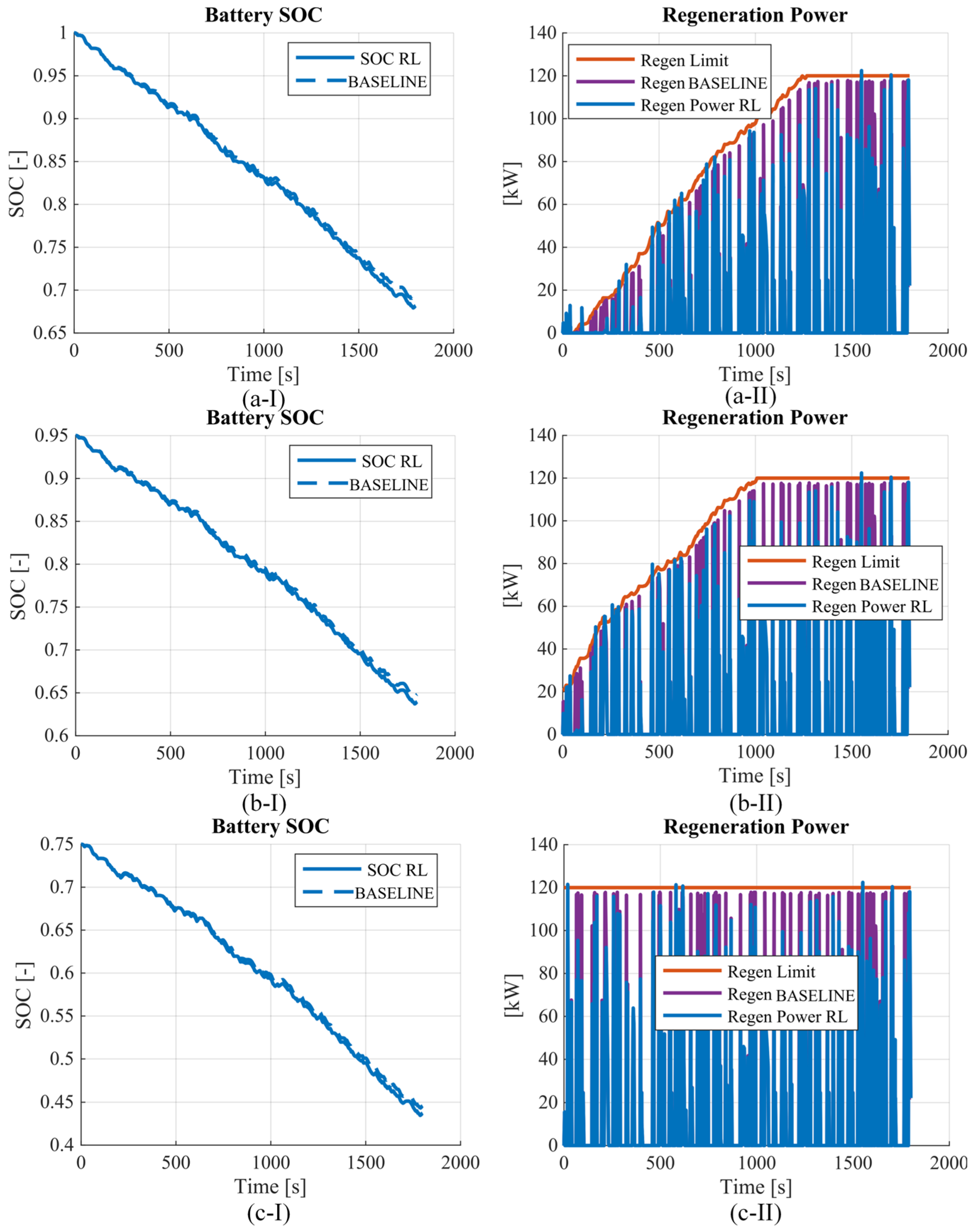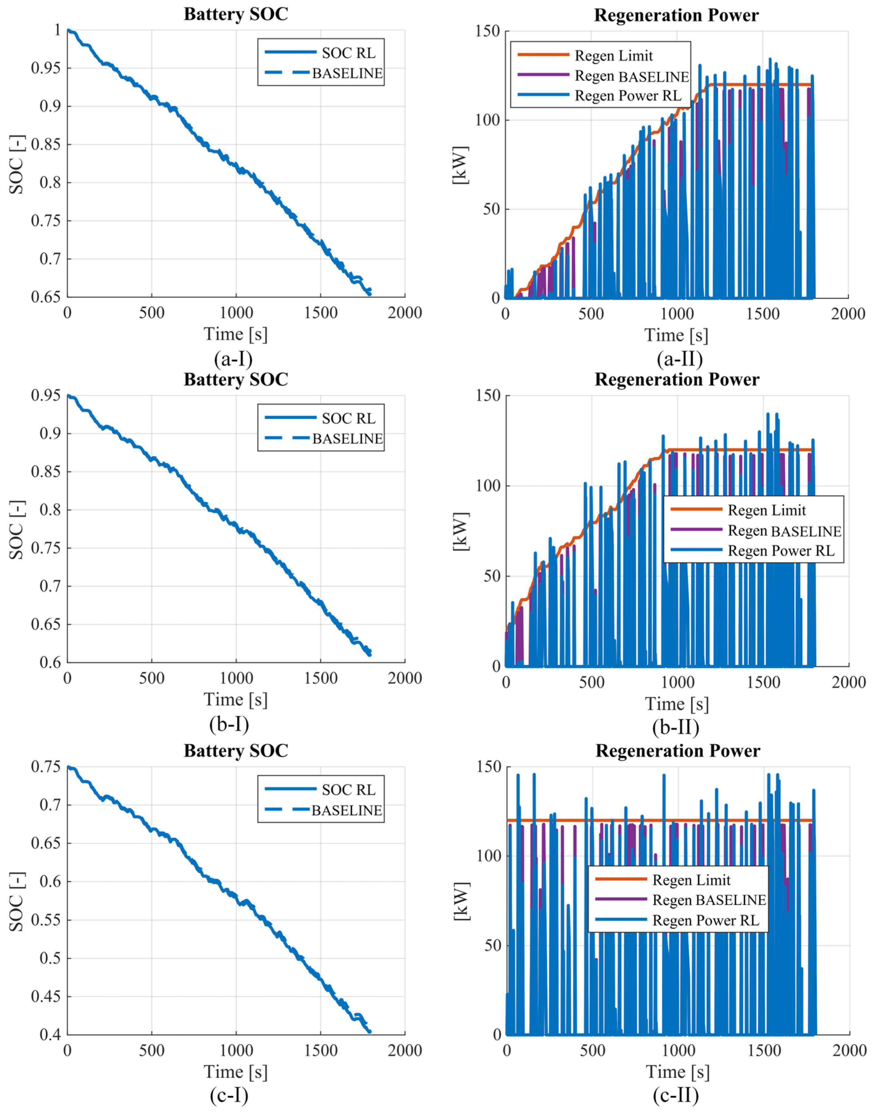Figure 18 shows the results in the random-rich driving cycle in different initial battery SoC conditions. The left-side plots show battery SoC evolution, while the right-side plots show the regenerative power P_regen considering different initial SoC levels, together with the SoP cap and the ideal baseline. The rule-based baseline is designed to approximate idealized control objectives (maximum achievable energy) under the given system constraints. This allows the evaluation to focus on the ability of the proposed RL approach to track the ideal behavior and quantify its relative performance gap.

Generally, the results suggest that the trained RL agent successfully tracks the SoP cap and only introduces a few short intervals of missed regenerative opportunity, seen as purple segments where the baseline controller applies more P_regen. The qualitative behavior is similar when the initial SoC values are 0.95 and 1. However, small initial overshoots are observed when the SoC is 1, which almost disappear when the initial SoC is 0.95. The tracking of P_cap in Figure 18(b-II) is also visibly tighter compared to Figure 18a. Remaining differences relating to the ideal reference mainly correspond to locally reduced P_regen and thus are small. With an initial SoC of 0.75, the controller clearly stays within the power cap throughout the cycle in Figure 18(c-II), but at the expense of more conservative behavior. Several braking events show that the RL agent selects less regenerative power than the ideal baseline, even when P_cap is not binding, which indicates additional lost opportunities but no aggressive use of the battery. Across all three initial SoC levels, the SoC trajectories of the RL controller and the ideal benchmark are nearly identical. This close agreement suggests that, despite local overshoots and occasional conservatism, the RL controller achieves the same net energy recovery as the idealized reference on the random drive cycle. For further validation, a more aggressive driver profile is simulated by increasing the proportional and integral gains of the driver block (PI controller, see (5)). This creates sharper accelerations and braking inputs, creating an opportunity to test the controllers’ resilience to high-frequency torque fluctuations and less predictable braking behavior. 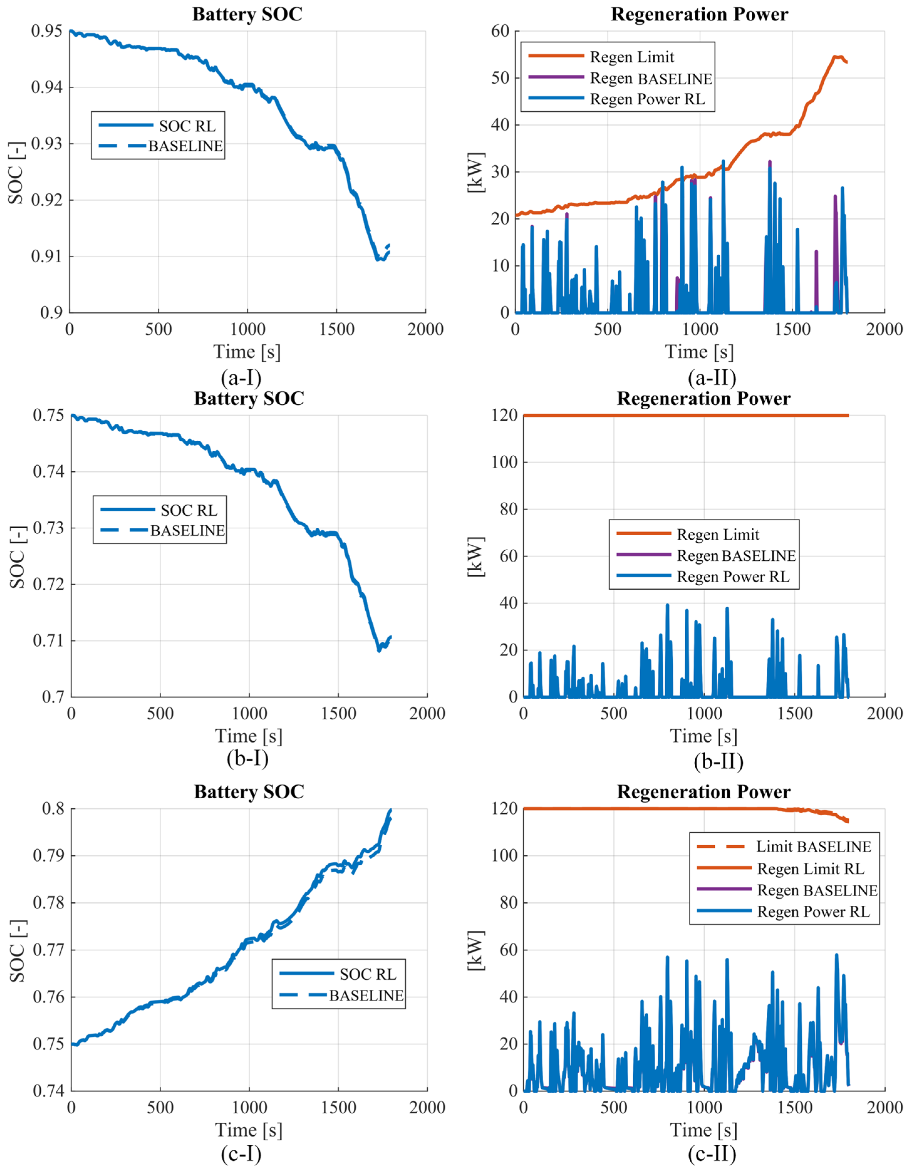Figure 19 shows the SoC (on the left) and regenerative power (on the right) trajectories for the alternative, more aggressive driver profile at the three initial SoC levels. Figure 19 generally shows that the SoC trajectories of the proposed RL controller and the ideal baseline remain almost indistinguishable.

This close agreement indicates that the net energy balance over the driving cycle is essentially preserved, and that the RL controller maintains comparable overall efficiency even under more aggressive driver behavior. This confirms that energy regeneration is successfully reached very close to the feasible range. However, as compared to the less-aggressive driving condition, the regeneration power curves (right side) show slight overshoots over P_cap during some braking incidents. While generally this suggests that the RL has been successfully trained to follow the defined objectives, the overshoot issue can be addressed directly by increasing the weight of the penalty term in the reward function or indirectly by integrating hard limits at the RL’s output gate. Typical results obtained when tested under the WLTP driving cycle are presented in Figure 20. Figure 20a,b show the results of the WLTP under flat road conditions. Moreover, Figure 20c corresponds to the results of WLTP with a simulated constant downhill slope of 5%, which is considered to investigate the controller behavior with sustained gravitational loading. Figure 20a shows that the RL regenerative power closely follows the ideal baseline, with only a few small overshoots of the limit around $t\approx 1000 \mathrm{s}$. The SoC trajectories are also almost identical, which means that the RL controller regenerates almost all the available energy during braking. When the start SoC was 0.75 in the flat WLTP simulation, the effective power remained almost constant. In this regime, all braking demand that can physically be handled by the electric motor is effectively recovered by regenerative braking. Figure 20c also confirms that in the presence of a constant downhill slope, the RL produces identical SoC and regenerative power trajectory to the ideal baseline, affirming the effectiveness of the trained RL controller.

Table 3. Summary of the numeric results.

Diving Cycle	Start SoC	RL Wh/km	Baseline Wh/Km	Diff [%]
WLTP 3 Flat	1	169.951	166.654	+1.98%
WLTP 3 Flat	0.95	138.079	133.854	+3.15%
WLTP 3 Flat	0.75	131.674	131.656	+0.01%
Random Cycle—Standard	1	496.994	483.182	+2.86%
Random Cycle—Standard	0.95	479.262	466.025	+2.84%
Random Cycle—Standard	0.75	463.654	450.632	+2.90%
Random Cycle—Aggressive	1	565.204	555.217	+1.80%
Random Cycle—Aggressive	0.95	548.733	540.330	+1.56%
Random Cycle—Aggressive	0.75	536.691	527.923	+1.66%

presents a summary of the numeric simulation results. The results suggest that the trained RL agent recovers almost all the regenerative energy available. For the WLTP3 case on the flat road, the control scheme is just about 2 and 3% less efficient than the ideal benchmark when the start SoC is 1 and 0.75, respectively. At the initial SoC of 0.75, the RL scheme closely follows the benchmark, demonstrating that it can recover almost all the regenerative energy available when the Pcap is not the limiting factor. For the random-rich driving cycle, the RL controller consistently consumes about 2.8–2.9% more energy than the benchmark across all start SoC levels. Altogether, it is seen that the proposed RL agent has been trained to successfully blend regenerative braking and frictional braking to achieve optimum recovery while meeting battery power criteria.

As for safety, the proposed approach uses a combination of learning and hard constraints to ensure it. The RL agent operates within a constrained environment, where the maximum allowable regenerative torque is explicitly bound by the battery SoP, motor limits, and operational constraints. These limits are computed at each time step and act as hard caps on the control output, which are learnt by RL. Additionally, rule-based fallback mechanisms remain active, ensuring that if RBS is not feasible or safe, friction braking fully compensates (as per the requirements of Section 2.2). Results under the edge test scenarios under intense decelerations (up to −4 m/s²) and high-SoC situations where battery charging limits are restrictive confirm that the regenerative torque rarely exceeds the SoP-imposed limits. It must also be noted that the RL controller does not govern the total braking force, but only the torque split. The required deceleration (and thus stopping distance) is enforced by higher-level controllers and tracking objectives. Such separation ensures that vehicle-level safety is guaranteed independently of the RL policy. Nevertheless, the challenges associated with certifying AI-based controllers under standards such as [28] and achieving the required Automotive Safety Integrity Levels (ASILs) are acknowledged. A pragmatic pathway toward adoption may involve hybrid control architectures, in which RL augments existing certified controllers rather than replacing them, thereby enabling incremental validation and regulatory acceptance.

While the proposed method is trained only on a limited driving cycle scenario, safety does not depend on generalization alone, since all actions are filtered through physical and control constraints at runtime. Even if the policy encounters unseen states, it cannot violate safety-critical limits due to these enforced bounds. While limited training data was used only to demonstrate the feasibility of the RL-based approach, it is possible to expand the RL training to consider more driving situations, considering new driving cycles and conditions, as outlined in the next Section.

6. Limitations of the Proposed Method and Potential Future Directions

As shown, RL facilitates an advantageous balance between competing objectives such as maximizing energy recovery, ensuring battery safety, and achieving smooth and comfortable braking performance. In principle, RL can be trained to provide even the possibility to adapt braking behavior to individual driver preferences and varying road conditions [35]. However, several important aspects remain to be addressed in the future. Further improvements can be achieved by enhancing the fidelity of the drivetrain and training models. Incorporating additional dynamics such as wheel and tire behavior, including slip and anti-lock mechanisms, would allow the controller to cover more realistic driving conditions. Moreover, modeling asymmetrical power losses between propulsion and regenerative braking modes, as well as integrating battery aging and thermal effects, are yet to be explored. While battery safety is indirectly considered through feasible power constraints, a dedicated battery lifetime model helps to assess how repeated braking events influence long-term battery health. The control objectives can also be expanded beyond energy recovery and battery power limits. A complete braking system should simultaneously account for vehicle stability, jerk minimization for ride comfort, and potentially individualized braking characteristics. These objectives can be embedded directly into the reward function, enabling the RL agent to learn an appropriate balance among multiple, and sometimes conflicting, criteria. Another promising extension involves distributing braking torque between axles and even individual wheels to support stability-oriented control strategies. Such an approach would allow closer integration with advanced vehicle dynamics systems and improve performance under low-friction or asymmetric road conditions. A systematic comparison with more recent RL algorithms (e.g., SAC) is an important direction for future work and will be considered to further assess potential gains in stability and sample efficiency. Finally, experimental validation and embedded implementation remain essential steps toward practical deployment. While direct deployment on an automotive ECU is beyond the current scope, the proposed approach is inherently lightweight, as the RL agent outputs only a single scalar control variable (i.e., torque-split factor), thereby limiting computational complexity compared to more elaborate policy structures. This characteristic supports the potential for real-time implementation, particularly when combined with standard embedded optimization techniques such as model quantization, pruning, and discretization. A laboratory prototype based on a scaled motor-generator setup is currently under development, with future work focusing on real-time implementation of the trained RL agent. Integration into the overarching RBS architecture, including coordination with actuator-level control loops, anti-lock braking systems, and supplementary stability control modules, should also be investigated to allow for a more synergetic assessment.

7. Conclusions

In this paper, the problem of optimal blending of the frictional and regenerative braking is studied. First, the braking problem is explored, and the operating requirements, considerations, and constraints, such as feasible regeneration regions by the electric motor, battery, and due to vehicle speed, as well as safety rules/regulations and fail-safes, are identified. Some of the identified requirements imply that, due to safety, existing controllers are designed in a conservative manner, resulting in regeneration potential being missed. To utilize the regeneration possibility to its full potential, more advanced controllers are needed to meet multiple control criteria simultaneously. To this end, the paper proposes that RL perform the blend control loop in the RBS control scheme. Training of the RL is fulfilled considering a digital twin model for the drivetrain of a Skoda Enyaq iV 80, established in MATLAB/Simulink. The RL’s reward function is shaped to maximize energy recovery while respecting the battery dynamic power limits and control smoothness. It is then exposed to synthetic braking scenarios emulating different braking scenarios, e.g., soft, moderate, and emergency braking. The test results on WLTP3 and random-rich driving cycles show that the RL successfully tracks the feasible regeneration energy available during braking while closely respecting battery SoP. The initial successful results demonstrate RL as a promising solution for integration in next-generation braking systems. The paper also provides a balanced discussion of potential limitations and outlines several directions for future work. Among other points, it highlights that although such schemes facilitate improved regeneration performance, safety must be ensured in accordance with the functional safety standard [28]. Consequently, future research should explore how AI-based methods, such as RL, can be integrated into BEV braking systems while respecting hard limits, implementing fail-safe mechanisms, and defining override strategies that revert the system to a safe baseline in case of RL instability, including reliable detection of such situations. This would likely require conducting a comprehensive Failure Mode and Effects Analysis (FMEA) to identify potential failure modes and appropriate mitigation techniques.