Fault Diagnosis of Rolling Bearings Based on an Ascending-Dimension Convolutional Neural Network

Abstract

Rolling bearings are critical and vulnerable components in mechanical equipment and are prone to various types of damage during operation. Consequently, rolling bearing fault diagnosis is of significant engineering importance. In recent years, deep learning-based approaches have achieved considerable progress in intelligent bearing fault diagnosis. However, existing models still suffer from several limitations, including insufficient feature extraction under noisy conditions, limited diagnostic accuracy, high computational cost, and low operational efficiency. To address these challenges, an intelligent rolling bearing fault diagnosis method based on an ascending-dimensional convolutional neural network (ADCNN) is proposed. Compared with conventional neural networks, the proposed ADCNN features a more compact model size, improved noise robustness, and higher diagnostic accuracy. A large convolutional kernel is introduced in the first layer to enhance noise immunity, while an ascending-dimensional module is employed to reduce the number of network parameters and improve feature extraction capability. In addition, a reduced linear transformation layer (RLTL) is incorporated to further achieve a lightweight architecture. Experimental results on the Case Western Reserve University (CWRU) dataset and a self-designed test dataset demonstrate that the proposed ADCNN achieves superior fault diagnosis performance under different noise environments while maintaining computational efficiency and model compactness.

1. Introduction

In recent years, fault diagnosis of rolling bearings has attracted attention due to its significance in maintaining industrial machinery. Traditional methods often struggle with noisy signals, leading to poor feature extraction. To address this, we propose an Ascending-Dimensional Convolutional Neural Network (ADCNN), which utilizes a larger convolutional kernel in the first layer and introduces a dimensional enhancement technique. These adjustments allow the network to better handle noisy environments, providing improved accuracy in fault diagnosis, even under challenging conditions.

With the improvement of industrialization and the rapid development of science and technology, rotating equipment is developing towards high-speed, large-scale, and automation directions [1]. Rolling bearings are not only essential components of rotating machinery but also vulnerable components in mechanical equipment. The health status of bearings has a significant impact on the performance, smooth operation, and service life of mechanical equipment [2,3]. Statistics have shown that about 44% of equipment failures are caused by rolling bearing failures [4]. Once a bearing fails, it will not only affect the operating efficiency of mechanical equipment but also cause economic losses and even threaten human life safety. Therefore, the fault diagnosis of rolling bearings has always been a focus of researchers [5,6,7].

The fault diagnosis of rolling bearings can be roughly divided into the following steps: (1) acquisition of vibration signals, (2) signal preprocessing, (3) extraction of useful feature information from the signals, and (4) fault modeling and diagnosis [8]. Traditional fault diagnosis methods are mainly based on signal analysis theory and are realized by improving the signal processing method. Wang et al. proposed a sparse guided empirical wavelet transformation method and successfully identified the resonance frequency band [9]. Kiral and Karagülle proposed a rolling bearing defect detection method for single and multiple defects based on finite element vibration analysis and established the relationship between bearing failure and vibration response [10]. Jiang et al. proposed a variational mode decomposition (VMD) method based on initial center frequencies (ICF-guided) to accurately extract weak damage features of rotating machinery [11]. The traditional signal processing method is of great significance in the fault diagnosis of rolling bearings and has provided important guidance for subsequent research. However, it is difficult to extract the feature signals manually using traditional fault diagnosis methods, and the work is further complicated if the bearing vibration signals are too complex [12]. Addressing this limitation has therefore become a key research objective.

Recent advancements in traditional methodologies continue to push the boundaries of fault diagnostics. For instance, Yang et al. [13] provided an in-depth analytical model for the time-varying excitation mechanism of bearing surface defects, offering a fundamental theoretical understanding that underpins many vibration-based diagnosis approaches. Furthermore, advanced signal processing techniques, such as the wavelet-supported residual processing method proposed by Melluso et al. [14] for the extraction of subtle torque faults in complex hybrid electric powertrains, demonstrate significant potential for robust extraction under challenging, noisy conditions. Despite these sophisticated developments, the reliance on expert knowledge for manual feature design and the computational complexity involved in processing highly non-stationary signals remain inherent limitations.

In recent years, data-driven bearing fault diagnosis methods have gradually developed. For example, the rolling bearing fault diagnosis method based on a multi-layer perceptron (MLP) [15,16] has played a certain role in solving the problems outlined above. Among many data-driven methods, the method based on deep learning has achieved certain results in bearing fault diagnosis [17]. Currently, a number of deep learning methods are commonly used, including transfer learning [18,19], deep residual networks (ResNets) [20,21], generating confrontation networks [22], deep confidence networks [23], convolutional neural networks [24] and so on. They have been successfully applied to computer vision [25], natural language processing [26], medical image diagnosis [27], automatic driving [28], etc. Janssens et al. [29] carried out early research on fault diagnosis based on the CNN architecture, converting the original signal into a frequency-domain signal through Discrete Fourier Transform (DFT) and inputting it into the CNN for model training. Compared to traditional diagnostic methods, the accuracy rate was improved by 6%. Xue F et al. [30] extracted depth features from the parallel multi-channel structures of 1D-CNN and 2D-CNN architectures, and they proposed a method to solve the problems of low accuracy of bearing fault diagnosis models and long network iteration times. Zhao B et al. proposed a new normalized CNN model for bearing fault diagnosis under complicated operating conditions in actual industrial scenarios [31]. In practical applications, there is a greater need for models that require less computer memory and have higher prediction efficiency. Common lightweight models include SqueezeNet [32], Xception [33], MobileNet [34], ShuffleNet [35], and deeply separable convolutional networks [36,37]. In actual operating conditions, bearings work in extremely severe environments, and it is inevitable that the noise will interfere with signals when acquiring vibration signals. The characteristic data of noise interference greatly reduces the accuracy rate in fault diagnosis. Therefore, it is also necessary to improve the noise resistance performance of the network (effectively extracting feature data from noisy signals and performing fault classification).

A fault diagnosis method based on ADCNN is presented in this paper to address the issues outlined above. The work done in this paper is summarized as follows:

(1)

A super convolutional kernel is used in the first layer, and an RLTL module is introduced in the tail layer of the network to improve the overall noise resistance and achieve a lightweight design.

(2)

Multiple sources of channel data are combined into two-dimensional data in parallel, using a 2D-CNN network in the spatial dimension of the two-dimensional channel and combining the weight-sharing mechanism to solve the information interaction problem while reducing the number of channels in the height direction and the feature information in the width direction, in addition to increasing the number of channels in the depth direction and achieving a network that is lightweight overall and improving the noise resistance performance.

(3)

The grouping convolution method is introduced to reduce the model’s parameters. The increased channel area is divided into three groups through a shuffle operation, further improving the feature extraction ability and network diagnosis accuracy of the convolution layer.

The rest of this paper is structured as follows. Section 2 covers the theoretical basis for improving the bearing fault diagnosis model. The architecture of the proposed bearing fault diagnosis network is described in detail in Section 3. A validation example of the model is presented in Section 3. The conclusion of this paper is revealed in Section 4.

Although simple fault detection is sufficient for deciding whether a bearing should be replaced, detailed fault-type identification provides additional value in practical engineering applications. Specifically, distinguishing between inner-race, outer-race, and rolling-element faults is beneficial for root-cause analysis, maintenance strategy optimization, and fault progression monitoring. Therefore, fine-grained fault diagnosis remains an important task in intelligent condition monitoring systems.

In addition to conventional CNN-based diagnostic pipelines, recent studies have explored transfer learning strategies for bearing diagnosis in industrial servomotor settings, as well as multi-size, wide-kernel convolution designs to enhance multi-scale feature extraction. Compared with these approaches, our ADCNN focuses on (i) improving noise robustness via a large-kernel frontend, (ii) reducing parameters through the ascending-dimension 2D weight-sharing design, and (iii) compressing the classifier using the RLTL module. These design choices jointly target robust and lightweight deployment.

Conventional 1D-CNN bearing diagnosis models typically rely on the stacking of 1D convolutions and frequent 1 × 1 pointwise convolutions to achieve cross-channel fusion. This often increases parameters rapidly with the channel number and does not explicitly exploit structured inter-channel correlations. In contrast, our ascending-dimension design reshapes the concatenated multi-channel 1D vibration segments into a 2D representation, enabling 2D convolutions to jointly model (i) temporal patterns along the signal axis and (ii) inter-channel correlation patterns along the newly formed spatial axis. Because 2D convolution shares weights across spatial locations, the proposed formulation provides stronger feature interaction with fewer parameters than repeated 1D fusion blocks, which is particularly beneficial under low-SNR conditions and for resource-constrained deployments.

Although this work focuses on robust single-domain training under a low SNR, the proposed ADCNN backbone can be naturally extended with transfer learning schemes to handle cross-machine or cross-condition adaptation in future work.

2. Materials and Methods

2.1. Theoretical Basis for Relevant Improvements

2.1.1. Theoretical Basis for the Influence of Convolutional Kernel Size on Network Noise Immunity

In the presence of noise, smaller convolutional kernels have a reduced receptive field, making it challenging to extract useful features from large vibration signals, especially in noisy conditions. By increasing the convolutional kernel size, we can achieve a larger receptive field, which helps in effectively extracting features from the input data while minimizing the impact of local noise. The proposed method uses large convolutional kernels in the first layer to increase noise immunity, especially in the presence of varying noise levels.

In actual operating conditions, the acquired fault signals are often accompanied by noise interference, which can affect the extraction of feature signals. Using large convolutional kernels is beneficial for eliminating local noise influence for the following reasons:

For convolutional neural networks, the main function of convolutional layers is to extract features from the input data. The neural network contains multiple convolutional layers, which transfer feature information hierarchically through the stack of multiple convolutional layers to achieve good feature extraction results. The convolutional layer is connected to the previous layer through local connections and weight sharing, which significantly reduces the number of parameters. The convolutional layer consists of several convolutional kernels, and each neuron in the convolutional layer is connected to multiple neurons located close to the region in the previous layer. The size of the region depends on the size of the convolutional kernel, which is called the receptive field. The larger the convolutional kernel, the larger the receptive field and the better the effect of extractable input features. The calculation formula of the receptive field is expressed as follows:

$$\begin{array}{c}{l}_k=l_{k-1}+\left[\left(f_k-1\right){\displaystyle \prod _{i = 1}^{k-1}}{s}_i\right]\end{array}$$

(1)

where l_k denotes the size of the receptive field at the k-th layer (in samples), l_{k − 1} denotes the size of the receptive field at the (k − 1)-th layer (in samples), f_k denotes the kernel size of the k-th convolution layer (in samples), s_k denotes the stride of the k-th layer, and k is the layer index. All symbols are summarized in the Nomenclature section. The principal calculation formula of the convolutional layer is expressed as follows:

$$\begin{array}{c} y_j=f\left({\displaystyle \sum _i}{X_i}^{*}{W}_{ij}+b_j\right)\end{array}$$

(2)

where $y_j$ denotes the j-th output feature map, $X_i$ denotes the i-th input feature map, W_ij denotes the convolution kernel connecting the i-th input channel to the j-th output channel, b_j denotes the bias term of the j-th output channel, * denotes the convolution operation and f(·) denotes the nonlinear activation function. All symbols are summarized in the Nomenclature section. $b_j$ represents the offset corresponding to the j-th output feature of the current convolution layer, while $f\left(x\right)$ is a nonlinear activation function. For the first layer of the network applied to rolling bearing fault diagnosis, $X_i$ represents the input vibration signal, which has a larger size in a single-dimensional direction, typically above 1000 [38], far exceeding the number of pixels in a single dimension of the image. Formula (1) indicates that the receptive field corresponding to small convolutional kernels is smaller, and it is inherently difficult to extract features from large vibration signals. The extraction effect of a small convolutional kernel for feature signals will deteriorate, especially when there is noise interference in the original input signals. Large convolutional kernels can be used to extract fault features of different fault types on a broader scale due to their larger receptive fields, eliminating the impact of local noise.

2.1.2. Theoretical Basis for Grouping Convolution

Grouping convolution is employed in this model to reduce the computational burden while maintaining the feature extraction performance. By splitting convolution kernels into groups, the number of operations is minimized, allowing for faster training and reduced model size, which is crucial for deployment in real-time fault detection applications.

Ordinary convolutional neural networks often impose a certain burden on computer hardware due to their large number of parameters and high demand for computing and data storage. Grouping convolution [39] is used for this model to reduce this burden, improve the operational efficiency of the model and build a lightweight network model. The reasons are outlined as follows:

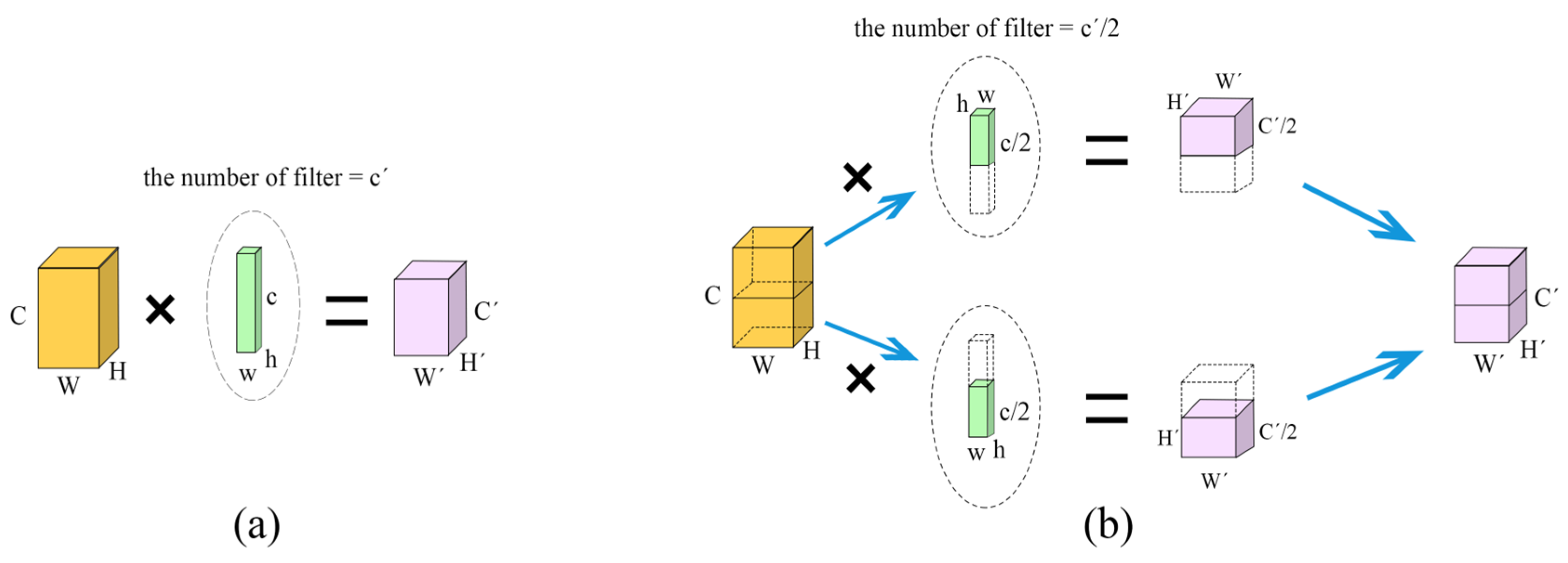
Figure 1 shows the difference between standard convolution and grouping convolution: In Figure 1a, depicting standard convolution, if the input feature is H $\times$ W $\times$ C, the number of convolutional kernels applied to the convolutional layer is C’, and the size of each convolutional kernel is h $\times$ w $\times$ c; at this point, the features of the input layer are converted to H’ $\times$ W’ $\times$ C’. For the grouping convolution shown in Figure 1b, each convolutional kernel group contains ${\displaystyle \frac{\mathrm{C}\mathrm{’}}{2}}$ convolutional kernels. Due to the molecules, the channel number of each convolutional kernel also becomes half of the original value, i.e., ${\displaystyle \frac{\mathrm{C}}{2}}$. Finally, the output feature of each convolutional kernel group after conversion is H’ $\times$ W’ $\times {\displaystyle \frac{\mathrm{C}’}{2}}$. The same effect as standard convolution is obtained after stacking.

The description above has shown that grouping convolution can achieve the same effect as standard convolution. According to the calculation, the parameter count of standard convolution is H $\times$ W $\times$ C $\times$ C’, while the parameter count of grouping convolution is H $\times$ W $\times {\displaystyle \frac{\mathrm{C}}{2}}\times {\displaystyle \frac{\mathrm{C}´}{2}}\times$ 2. The parameter count is reduced to 1/2 of the original value. The training results do not tend to be over-fitted, and the effect of a lightweight network is achieved by reducing the training parameters in this way.

2.1.3. Theoretical Basis for Channel Shuffle

For the bearing fault diagnosis signal features, the channel shuffle method is used for feature shuffling, which promotes information fusion between channels and improves the feature extraction ability of convolutional layers. The specific reasons are described as follows:

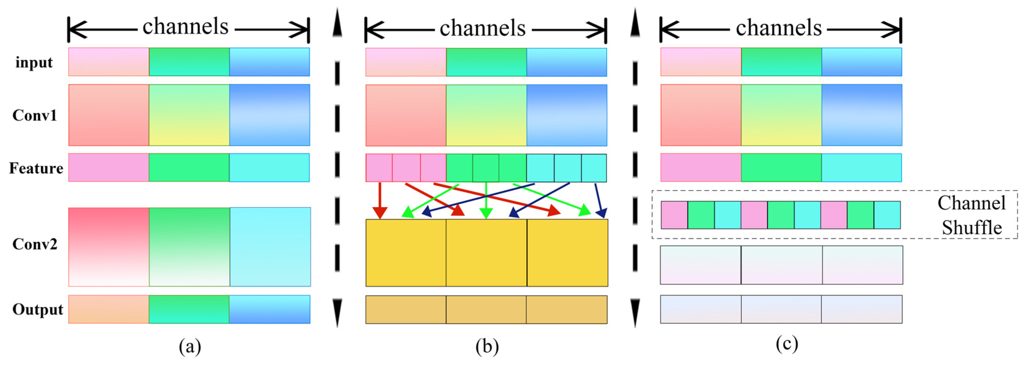
In a broad sense, convolutional operations include three processes, i.e., convolutional operations, batch standardization and nonlinear activation. A conventional CNN model entails a process in which convolution continuously reduces the feature size and increases the number of channels. The number of channels is the number of convolutional kernels, as well as the number of different abstract modes. The channel contains information about the adaptation of a mode to the data of the previous layer. A set of adaptation information can be weighted and mapped to multiple channels, and multiple sets of adaptation information can also be mapped to multiple channels. However, multiple sets of adaptation information being aggregated in a single channel will cause confusion and mutual interference of the adaptation information. Full channel convolution is used in traditional CNNs, as shown in Figure 2a. This would hinder the information flow and reduce the ability to express features if there is no pointwise 1 $\times$ 1 convolution or channel shuffle, and the final output features are only calculated from a portion of the input channel features. In practical work, we expect that the channel information between feature maps can be fused after the convolution of a group, as shown in Figure 2b, and the features of each group can be dispersed into different groups before proceeding with the next group of convolution. The channel shuffle method (Figure 2c) scrambles the channel order of the output results after the first pointwise group convolution so that the feature information of the output channels no longer only comes from a small portion of the input channels, that is, the output channels and the input channels are completely correlated.

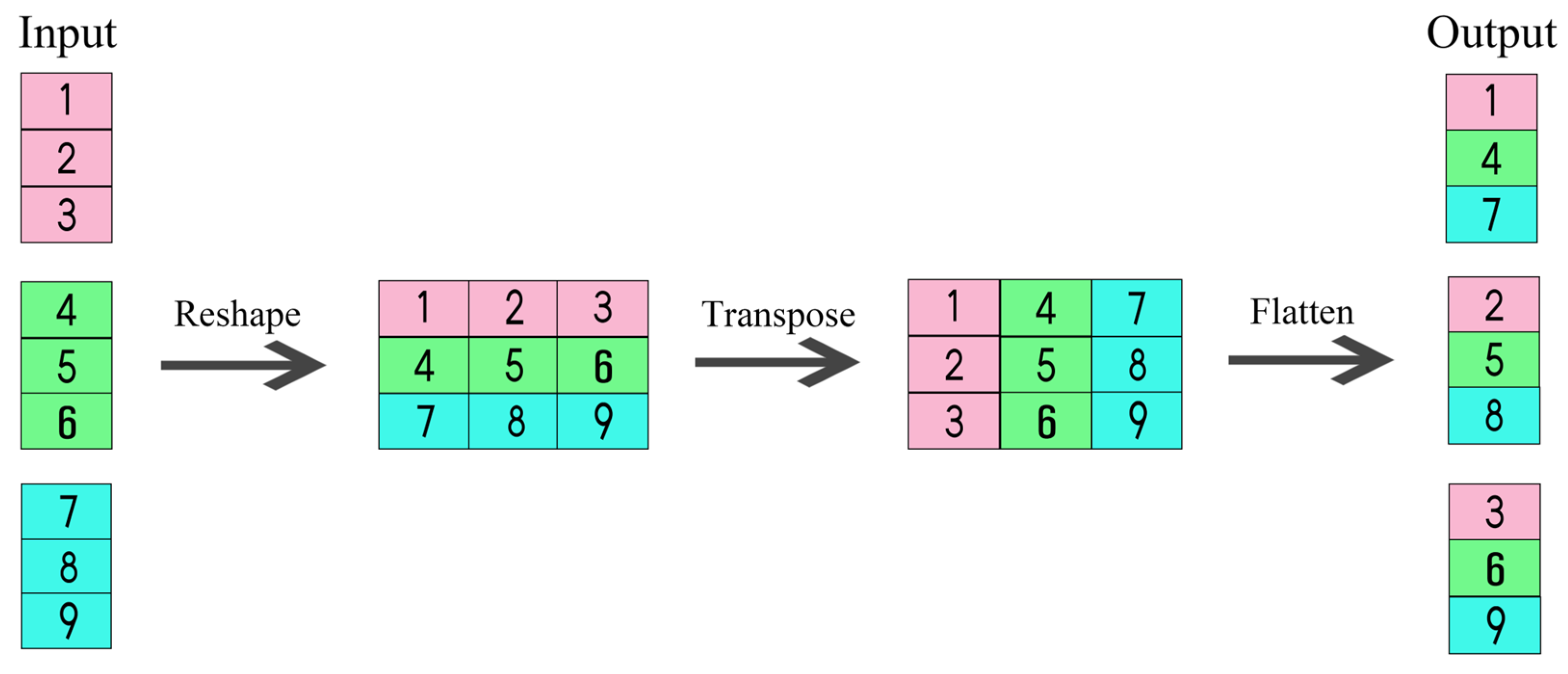
The specific implementation of channel shuffle is achieved through several conventional tensors, as shown in Figure 3, divided into three steps: (1) Reshape: First, the input channel is reshaped from one dimension into two dimensions; one is the number of convolutional groups, and the other is the number of channels contained in each convolutional group. (2) Transpose: The two expanded dimensions are replaced. (3) Flatten: The final channel shuffle can be completed after the replaced channels are flattened. After the channel shuffle, the features do not correspond to channels; instead, all channels are correlated. This promotes information fusion between the channels and is more conducive to feature signal extraction.

2.1.4. Theoretical Basis for Weight Sharing

Based on the parallel combination of multiple pieces of channel data into two-dimensional data, using a 2D-CNN network in the spatial dimension of the two-dimensional channel, in combination the weight-sharing mechanism, to solve information interaction problems can effectively reduce the network weight parameters and achieve an overall lightweight design of the network. The reasons are presented as follows:

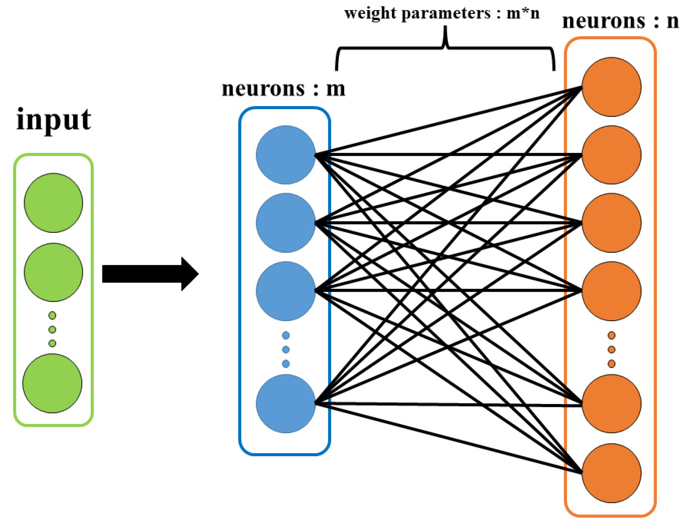
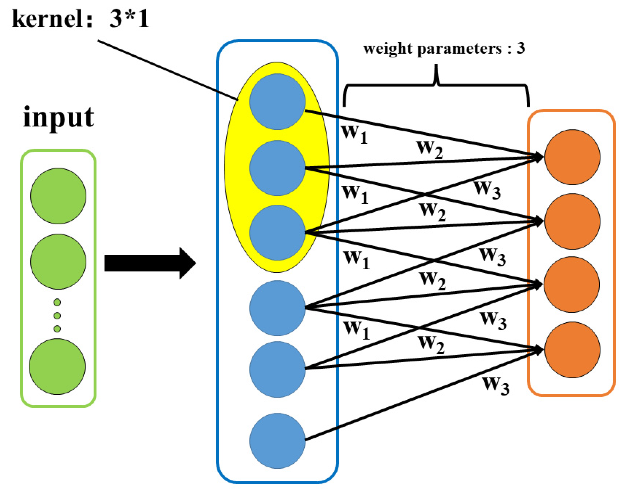
For a neural network, a lightweight design is closely related to the operational efficiency of the network. Making the network lightweight is an unavoidable issue in engineering applications. In general, the form of a full connection is used for the connection between layers of the neural network, as shown in Figure 4. Each neuron is connected to all neurons in the previous layer, and the weights of these connecting lines are independent of other neurons. It is assumed that the previous layer has m neurons and the current layer has n neurons. Then, the weight parameter in the entire calculation process is m $\times$ n.

For convolutional neural networks, weight sharing is an important feature that can reduce weight parameters. As shown in Figure 5, when extracting features, the convolution kernel moves from the head of the input feature to the tail according to the step size set by the network. For single-channel signal features, this process is completed by a single convolutional kernel, so the weight parameter of the entire process is the size of the convolutional kernel, as shown in the figure as 3. If a full connection is used, the parameter is 24. Obviously, this feature reduces the number of parameters and results in lightweight network to some extent.

Similarly, this property can also be applied to multiple channels. Parallelizing multiple pieces of channel data into two-dimensional data and utilizing the weight-sharing property of 2D-CNN can effectively reduce the network weight parameters. The specific operations are described in detail in Section 2.

2.2. The Proposed Bearing Fault Diagnosis Network Architecture

2.2.1. Model Architecture and Training Process

The proposed Ascending-Dimension Convolutional Neural Network (ADCNN) architecture consists of several key components: a large convolutional kernel module, an ascending-dimension module, an RLTL module, and standard convolutional pooling layers. The input to the network is a one-dimensional vibration signal, which is processed through multiple convolution and pooling layers, ultimately leading to fault-type classification.

Large Convolutional Kernel Module

To improve noise resistance, the first layer of the ADCNN uses a large convolutional kernel (e.g., 513-sized convolutional kernel). This approach allows the network to capture features from a larger area of the input signal, thereby reducing the impact of local noise interference. The use of large convolutional kernels is essential for feature extraction when the input signal is affected by noise, as it helps the network to focus on broader patterns in the data.

Ascending-Dimension Module

The primary motivation behind the ascending-dimensional module is to address the inefficiency of standard 1D-CNNs in processing multi-channel bearing vibration data. Conventional approaches often rely on pointwise (1 × 1) convolutions for cross-channel fusion, which can cause a rapid growth in parameters as the channel count increases and may fail to exploit inter-channel correlation structures. Therefore, we transform the concatenated multi-channel 1D signals into a 2D representation, enabling subsequent 2D convolutions to capture both intra-channel temporal patterns and inter-channel correlations within a unified feature-learning framework. Importantly, the weight-sharing property of 2D convolutions across the newly formed spatial dimension reduces parameters compared with stacked 1D convolutions, making the model lighter yet more expressive, which is particularly beneficial under noisy conditions.

We introduce an ascending-dimension module to expand the feature space. Initially, the feature dimensionality is increased by using a depth-wise expansion mechanism. The number of channels is first expanded from 16 to 48. This allows the model to focus on different aspects of the feature map, improving the network’s ability to capture meaningful patterns while maintaining efficiency. In the subsequent convolution layers, we use a 2D convolutional network (2D-CNN) to process these features in a higher spatial dimension, facilitating more effective feature extraction.

Compared with (i) purely stacked 1D-CNNs and (ii) channel fusion-heavy designs using repeated 1 × 1 convolutions, the ascending-dimension 2D formulation allows ADCNN to exploit inter-channel correlations with fewer parameters. This is especially beneficial for deployment under resource constraints and in low-SNR environments, where a compact model with a large receptive-field frontend is preferred.

RLTL Module

In traditional convolutional neural networks (CNNs), the fully connected (FC) layers typically consume many parameters and computation resources. To address this, we propose the RLTL (Reduced Linear Transformation Layer) module, which is based on Kronecker product decomposition. This module significantly reduces the size of the fully connected layers while maintaining or improving the network’s performance. It allows the model to maintain efficiency in terms of both parameter count and computational cost. The RLTL module replaces traditional FC layers, and the computational cost is reduced by decomposing the weight matrices, leading to a lighter network architecture without sacrificing fault diagnosis accuracy.

Training Process

The model is trained using the Adam optimizer with an initial learning rate of 0.001. To further ensure the robustness and generalizability of the model, 5-fold cross-validation (k = 5) is employed, where the dataset is divided into five subsets. In each fold, one subset serves as the test set, and the remaining four subsets are used for training. This approach ensures the model is validated across different data combinations, reducing the risk of overfitting and providing a more reliable performance measure. Cross-validation (k-fold cross-validation) is employed to ensure that the model generalizes well to unseen data. The data is split as follows: 80% for training and 20% for validation.

To prevent overfitting, we use data augmentation, specifically employing sliding window sampling techniques. For clarity, k-fold cross-validation is used for performance evaluation, while the reported test accuracy refers to the held-out fold in each validation round. The use of k-fold cross-validation inherently evaluates the model across multiple data subsets, and the reported results represent averaged performance over different validation folds, thereby reducing sensitivity to a single data split.

Hyperparameter Tuning

Hyperparameters such as the kernel size, learning rate, batch size, and number of convolutional layers were optimized using grid search and random search. The final selection of hyperparameters was based on performance metrics from the validation set. The hyperparameter search ranges were empirically determined based on preliminary experiments, and validation accuracy was used as the primary criterion for model selection.

2.2.2. Dataset Description and Preprocessing

For this study, we used the Case Western Reserve University (CWRU) dataset and our designed test dataset. The data includes vibration signals from rolling bearings under different fault conditions: healthy, inner-ring fault, outer-ring fault, and rolling fault.

Data Preprocessing: Before feeding the data into the network, we applied standardization to normalize the vibration signals. Gaussian white noise with different signal-to-noise ratios (SNRs) ranging from −5 dB to +5 dB was added to simulate real-world noise interference. The preprocessed data was then split into training and test sets (80% for training and 20% for testing).

Data Augmentation: To increase the number of training samples, we used the sliding window sampling method. The window size was set to 128, and the overlap between consecutive windows was set to 50%. This helps in capturing the time-series nature of the signal and reduces the risk of overfitting.

Dataset Example

The data from CWRU includes different fault types (inner-ring fault, outer-ring fault, and rolling fault) with varying damage sizes (7 mil, 14 mil, and 21 mil). The total length of the signals was determined to be 1024 samples, and this sample length was chosen to capture enough information to perform accurate fault diagnosis.

Hyperparameter Selection

The selection of hyperparameters (such as the kernel size, number of layers, learning rate, and batch size) was done based on validation performance. We used a combination of grid search and random search to find the optimal configuration. The learning rate was initially set to 0.001 and reduced by 10% after every 10 episodes. The batch size was set to 32, which balances training speed and model performance.

2.2.3. Construction of Ascending-Dimensional Module Based on Weight-Sharing Theory

The ascending-dimensional module is designed to enhance feature extraction efficiency while reducing computational overhead. This is achieved through grouping convolutions that reduce the dimensionality of feature maps, followed by the use of 2D-CNN layers that operate on higher-dimensional data, significantly improving the network’s ability to learn complex patterns in fault data while minimizing the number of parameters.

The primary motivation behind the ascending-dimensional module is to address the inefficiency of standard 1D-CNNs in processing multi-channel bearing vibration data. Conventional approaches rely heavily on pointwise (1 × 1) convolutions for cross-channel information fusion, which, while effective, lead to a quadratic increase in parameters with channel count and fail to exploit potential spatial correlations among channels. Our method transforms the concatenated multi-channel 1D signal into a 2D representation. This allows the subsequent 2D convolutional layers to capture both intra-channel temporal patterns and inter-channel correlation structures simultaneously within a unified spatial-feature learning framework. Crucially, the weight-sharing property of 2D convolution across the newly formed spatial dimension dramatically reduces parameters compared to using multiple stacked 1D convolutions, making the network both lighter and more powerful in feature extraction, which is particularly advantageous under noisy conditions.

From the weight-sharing theory in Section 2, we can see that the weight-sharing feature of convolutional neural networks can effectively reduce the weight parameters, thereby reducing the network calculation workload, and lighten the network model. For a 1D-CNN, the calculation process of the parameter count of the convolutional layer is expressed as follows:

$$\begin{array}{c} p_w=k\times c_i\times c_o\end{array}$$

(3)

$$\begin{array}{c} p_b=c_i\times c_o\end{array}$$

(4)

$$\begin{array}{c} p=p_w+p_b=\left(k\times c_i+1\right)\times c_o\end{array}$$

(5)

where p_w denotes the number of convolution weight parameters (dimensionless count), p_b denotes the number of bias parameters (dimensionless count), k denotes the kernel size of the convolution layer (in samples), C_in denotes the number of input channels, and C_out denotes the number of output channels. All symbols in Equation (5) are summarized in the Nomenclature section. The calculation process of the convolutional layer’s floating-point operations (FLOPs) is expressed as follows:

$$\begin{array}{c} f_m=k\times c_i\end{array}$$

(6)

$$\begin{array}{c}{ f}_a=\left(k-1\right)\times c_i+\left(c_i-1\right)+1=k\times c_i\end{array}$$

(7)

$$\begin{array}{c} Flops=\left(f_a+f_m\right)\times c_o\times l_o=\left(2\times k\times c_i\right)\times c_o\times l_o\end{array}$$

(8)

where $f_m$ denotes the number of multiplication operations, $f_a$ denotes the number of addition operations and $l_o$ denotes the output feature length (in samples). All symbols used in this equation are summarized in the Nomenclature section.

Equations (5) and (8) indicate that the CNN parameters and operations are mainly concentrated in layers with many channels. Many convolutional layers with K = 1 are used for channel information interaction to ensure the mapping relationship between the channels. However, secondary and tertiary mappings between channels do not increase the number of channels while convolving, thereby reducing the degree of matching with the original input data. By sharing weights and enhancing the dimensions of output data, convolution outputs several or a series of abstract patterns during training, making the training process more targeted and greatly reducing the number of parameters. Currently, for the mapping relationship between channels in CNN models, the weight-sharing and dimension promotion principles of CNNs in data feature length can also be used to enhance the spatial dimension of channels, and the weight-sharing method can be used between the channels.

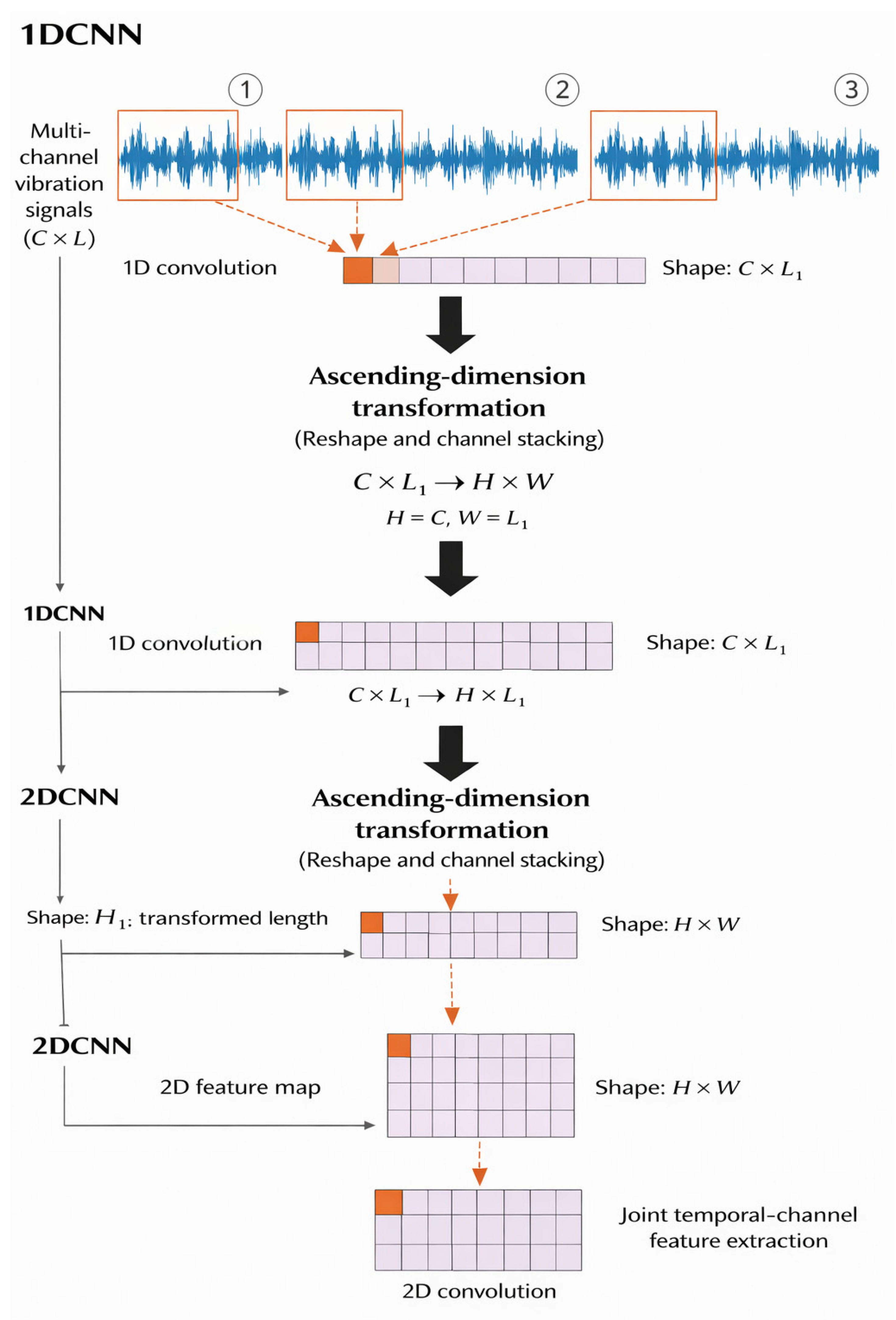
For a 1D-CNN, the channel change, in the usual sense, refers to the process in which the number of channels changes with the number of convolutional kernels after the input data passes through the convolutional layer. After the number of channels changes, feature information can be extracted more accurately using a 2D-CNN. The process of transforming a channel from a one-dimensional space to a two-dimensional space that can be convolutionally operated using a 2D-CNN is also a process of enhancing the spatial dimension of the channel. Based on the theory described above, an ascending-dimension convolutional module that combines the number of channels and feature signals into two-dimensional data is proposed in this paper. First, the size of the feature information is reduced significantly by using grouping convolution; then, a 2D-CNN is used to focus on the processing of channel issues in the convolution process in a higher spatial dimension. The principle of channel dimension promotion is shown in Figure 6.

2.2.4. RLTL Module Construction Based on Kronecker Product Decomposition

The fully connected layer is generally placed in the end layer of the convolutional neural network, playing the role of “classifier” in the entire convolutional neural network. Its essence is to transform from one feature space to another. Any dimension of the target space is affected by each dimension of the source space. In the fault diagnosis task of rolling bearings, the full connection layer plays the role of final classifier.

The fully connected layer, as an important component of the CNN model, often accounts for most of the parameters and computational complexity of the model. We propose an RLTL module as an improved form of the fully connected layer to achieve the goal of lightweight networks. The theoretical basis for the improvement is the Kronecker product decomposition theory.

The Kronecker product is also known as the tensor product or direct product. Its basic formula is expressed as follows:

$$\begin{array}{c}A\otimes B=\left[\begin{array}{ccc}{a}_{11}B& \dots & a_{1n}B\\ ⋮& \ddots & ⋮\\ a_{m1}B& \dots & a_{mn}B\end{array}\right]\in R^{mp\times nq}\end{array}$$

(9)

where $A=\left(a_{ij}\right)\in {\mathbb{R}}^{m\times n} ,B=\left(b_{ij}\right)\in {\mathbb{R}}^{p\times q}$. The matrix dimension obtained after the operation is the product of the two matrix dimensions involved in the operation $(mp\times nq)$. The specific calculation process is expressed as follows:

$$\begin{array}{c}A\otimes B=\left[\begin{array}{cc}\begin{array}{cc}\begin{array}{ccc}{a}_{11}{b}_{11}& a_{11}{b}_{12}& \dots \\ a_{11}{b}_{21}& a_{11}{b}_{22}& \dots \\ ⋮& ⋮& \ddots \end{array}& \begin{array}{cc}{a}_{11}{b}_{1q}& \dots \\ a_{11}{b}_{2q}& \dots \\ ⋮& \end{array}\\ \begin{array}{ccc}{a}_{11}{b}_{p2}& a_{11}{b}_{p2}& \dots \\ ⋮& ⋮& \end{array}& \begin{array}{cc}{a}_{11}{b}_{pq}& \dots \\ ⋮& \ddots \end{array}\end{array}& \begin{array}{cc}\begin{array}{cc}\dots & a_{1n}{b}_{11}\\ \dots & a_{1n}{b}_{21}\\ & ⋮\end{array}& \begin{array}{ccc}{a}_{1n}{b}_{12}& \dots & a_{1n}{b}_{1q}\\ a_{1n}{b}_{22}& \dots & a_{1n}{b}_{2q}\\ ⋮& \ddots & ⋮\end{array}\\ \begin{array}{cc}\dots & a_{1n}{b}_{p1}\\ & ⋮\end{array}& \begin{array}{ccc}{a}_{1n}{b}_{p2}& \dots & a_{1n}{b}_{pq}\\ ⋮& & ⋮\end{array}\end{array}\\ \begin{array}{cc}\begin{array}{ccc} ⋮& ⋮& \\ a_{m1}{b}_{11}& a_{m1}{b}_{12}& \dots \end{array}& \begin{array}{cc}⋮& \\ a_{m1}{b}_{1q}& \dots \end{array}\\ \begin{array}{ccc}{a}_{m1}{b}_{11}& a_{m1}{b}_{22}& \dots \\ ⋮& ⋮& \ddots \\ a_{m1}{b}_{p1}& a_{m1}{b}_{p2}& \dots \end{array}& \begin{array}{cc}{a}_{m1}{b}_{2q}& \dots \\ ⋮& \\ a_{m1}{b}_{pq}& \dots \end{array}\end{array}& \begin{array}{cc}\begin{array}{cc}\ddots & ⋮\\ \dots & a_{mn}{b}_{11}\end{array}& \begin{array}{ccc}⋮& & ⋮\\ a_{mn}{b}_{12}& \dots & a_{mn}{b}_{1q}\end{array}\\ \begin{array}{cc}\dots & a_{mn}{b}_{21}\\ & ⋮\\ \dots & a_{mn}{b}_{p1}\end{array}& \begin{array}{ccc}{a}_{mn}{b}_{22}& \dots & a_{mn}{b}_{2q}\\ ⋮& \ddots & ⋮\\ a_{mn}{b}_{p2}& \dots & a_{mn}{b}_{pq}\end{array}\end{array}\end{array}\right]\end{array}$$

(10)

The properties of Kronecker product are shown in the following formula:

$$\begin{array}{c} vec\left(Y\right)=vec\left(PXQ\right)=\left(Q^T⨂P\right)vec\left(X\right)\end{array}$$

(11)

where P, Q and Y are given matrices; X represents unknown matrices; and $PXQ=Y$ has a unique solution. $vec\left(·\right)$ represents the straightening operator of a matrix, which is a column vector formed by stacking all the columns of the matrix. The operation process of the FC layer includes three steps: linear operation, batch standardization, and activation. To simplify the derivation process, only the linear operation part of a single sample is considered, and the bias parameter is not considered. The linear operation of the FC layer can be understood as a weighted process, which can be expressed in the following form:

$$\begin{array}{c}y=Wx\end{array}$$

(12)

In this form, $x\in {\mathbb{R}}^{m\times 1}$ and $y\in {\mathbb{R}}^{n\times 1}$ are column vectors and $W\in {\mathbb{R}}^{n\times m}$ is a weight matrix. Let x and y be the straightened vectors of matrices X and Y; then, $x=vec\left(X\right)$ and $y=vec\left(Y\right)$. At this point, $X\in {\mathbb{R}}^{m_1\times m_2}$ and$Y\in {\mathbb{R}}^{n_1\times n_2}$. Combining Equations (10) and (11), it is concluded that a unique solution for $PXQ=Y$ is equivalent to a unique solution for $y=vec\left(PXQ\right)$.

Realization of the process expressed as $y=vec\left(PXQ\right)$ is completed in the following 3 steps:

Step 1, linear operation with X as input:

$$\begin{array}{c} Y_1=AX\end{array}$$

(13)

Step 2, transposition operation:

$$\begin{array}{c} Y_1^T=X^T{A}^T\end{array}$$

(14)

Step 3, linear operation with $Y_1^T$ as input:

$$\begin{array}{c} Y_2=B{Y}_1^T=B{X}^T{A}^T\end{array}$$

(15)

Equation (15) is equivalent to

$$\begin{array}{c}vec\left(Y_2\right)=vec\left(B\right)X^T{A}^T\end{array}$$

(16)

Taking $y=vec\left(Y_2\right)$ into account, in combination with Formula (11), the following results are obtained:

$$\begin{array}{c} y=vec\left(Y_2\right)=vec\left(B{X}^T{A}^T\right)=\left(A⨂ B\right)vec\left(X\right)=\left(\mathrm{A}⨂B^T\right)x\end{array}$$

(17)

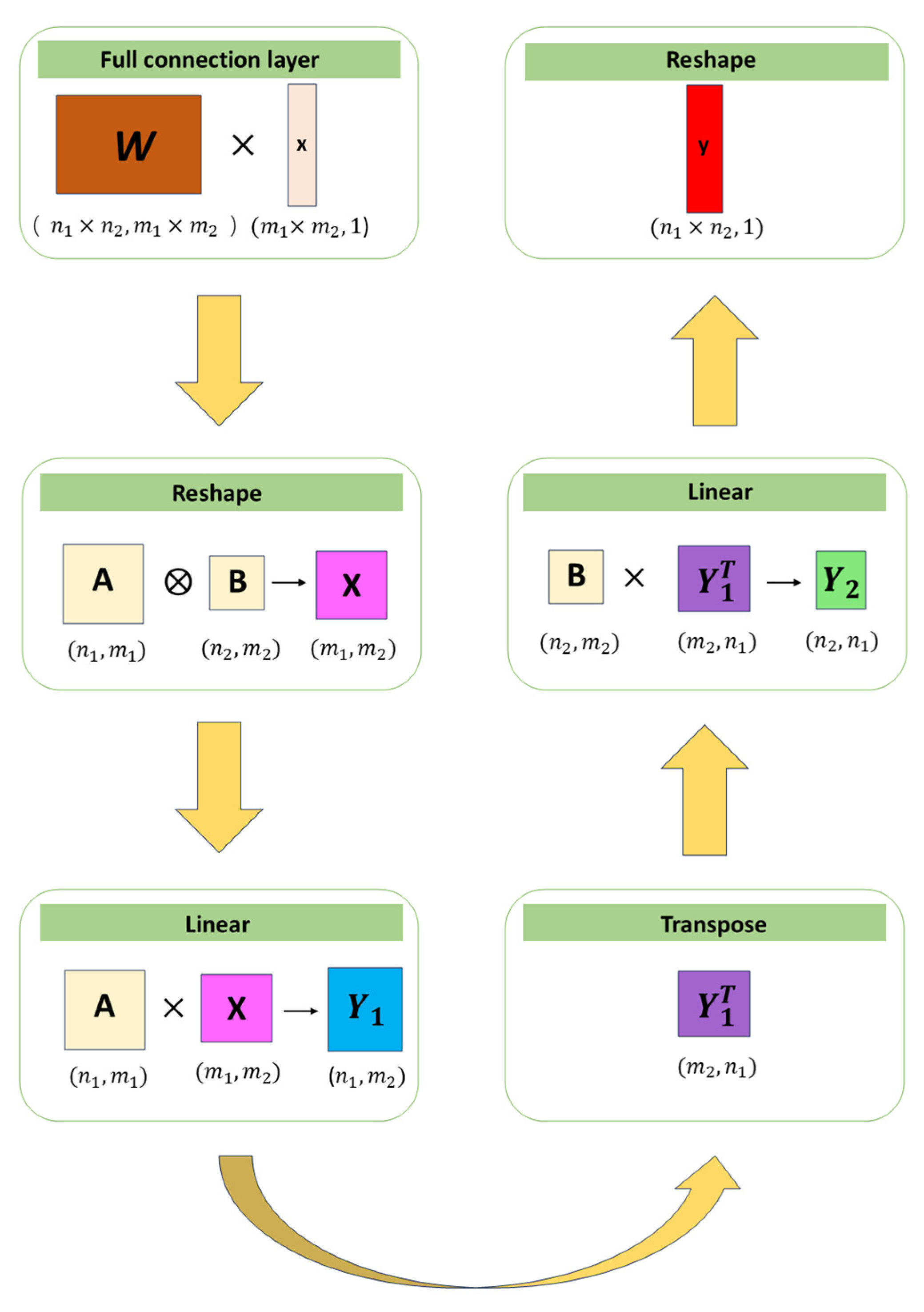
The derivation above shows that the entire process involves several subprocesses—namely, conversion, weighting, transposition, weighting, and conversion—achieving equivalent transformation of the full connection layer. The process described above can also be referred to as decomposition of the full connection-layer weight matrix. A schematic diagram of the entire process is shown in Figure 7.

By observing and analyzing the equivalent transformation process between the Kronecker decomposition and the fully connected layer described above, it is not difficult to find that decomposing the weight matrix can convert a single linear operation of the FC layer into two linear operations. Compared to the original weight matrix (W), the sizes of the two decomposed weight matrices (A and B) are greatly reduced. Based on this principle, an RLTL module is proposed to improve the full connection layer. The pseudocode of the RLTL module is shown in

Table 1. RLTL module pseudocode.

RLTL Module
1. input data: $\mathit{x}\in {\mathbb{R}}^{m\times 1}$
2. output data: $\mathit{y}\in {\mathbb{R}}^{n\times 1}$
3. weight matrix: $\mathit{A}\in {\mathbb{R}}^{n_1\times m_1}$, $\mathit{B}\in {\mathbb{R}}^{n_2\times m_2}$
4. bias: $\mathit{b}\in {\mathbb{R}}^{n\times 1}$
5. activation function: $\sigma ( )$
6. $\mathit{X}\leftarrow {vec}^{-1}\left(\mathit{x}\right)$
7. $\mathit{Y}\leftarrow \mathit{A}\mathit{X}$
8. $\mathit{X}\leftarrow {\mathit{Y}}^T$
9. $\mathit{Y}\leftarrow \mathit{B}\mathit{X}+\mathit{b}$
10. $\mathit{y}\leftarrow {vec}^{-1}\left(\mathit{Y}\right)$
11. $\mathit{y}\leftarrow \sigma (\mathit{y} )$

.

The Kronecker decomposition process is very complicated. Considering the weight matrices (W), A and B can also be continuously updated during the backpropagation process during actual execution; then, after designing the dimensions of A and B, the network can update A and B by itself through two operations. This also allows the model to determine the optimal weight parameters by itself under supervised learning. This operation can effectively improve the running efficiency of the mode.

2.2.5. Construction of the Overall Model of ADCNN

The structure and corresponding parameters of the ADCNN designed in this paper are shown in

Table 2. ADCNN.

	Layer	Input Channels	Output Channels	Kernel Size	Stride	Padding	Group
1	Con1d+BN+RELU	1	16	513	1	1	1
2	Con1d+BN+RELU	16	48	3	1	1	16
3	Shuffle channel	–	–	–	–	–	16
4	Unsqueeze	–	–	–	–	–	–
5	Con2d+BN+RELU	1	4	(2, 3)	(2, 2)	(0, 1)	1
6	Avgpool2d	–	–	(1, 2)	(1, 2)	–	–
7	Con2d+BN+RELU	4	16	(2, 3)	(2, 2)	(0, 1)	4
8	Avgpool2d	–	–	(1, 2)	(1, 2)	–	–
9	Con2d+BN+RELU	16	64	(2, 3)	(2, 2)	(0, 1)	16
10	Avgpool2d	–	–	(1, 2)	(1, 2)	–	–
11	Con2d+BN+RELU	64	256	(2, 3)	(2, 2)	(0, 1)	64
12	Adaptive Avgpool2d	–	–	–	–	–	–
13	RLTL	–	4	–	–	–	–

. Its Layer 1 and Layer 2 (in this paper, the convolutional layer relates to the standardization layer and the ReLU layer) are lightweight improvements to the 1D-CNN with 1 input channel and an 16 output channels, using a super convolution kernel and a grouping convolution method. Edge padding is used on the feature length for Layer 2 and the subsequent layers, which reduces the feature size an integral number of times. Pointwise convolution is not used for Layer 3; channel shuffle is used instead. This is because in Layer 2, 16 input channels are expanded to 48 output channels (that is, each input channel is mapped to 3 output channels), and the subsequent adjacent channel downsampling ultimately integrates and maps these 3 channels to 1 channel. Due to the importance of the first-layer information, 48 output channels are divided into 3 parts in the model. Each part (16 channels) corresponds to a feature that is mapped to 16 input channels.

Layer 4 is an ascending-dimension network module, and Layers 5, 7, 9 and 11 are 2D-CNN layers. A downsampling of s = 2 is performed in each layer of convolution on both the height and width data dimensions while increasing to four times the number of channels in the depth direction. Taking Layer 5 as an example, when performing convolutional operations, 48 input channels share a convolutional kernel of K = (2, 3), which is equivalent to performing a step convolutional operation of s = 2 on 48 input channels in the height direction, that is, sharing weights on 48 input channels. Layers 6, 8 and 10 are average pooling layers, with the feature size in the width direction reduced by half and the number of channels in the height and depth directions unchanged. RLTL modules are used in Layer 13 to replace traditional FC layers. Only one layer of RLTL modules is used, as the number of channels in the depth direction after convolution is only 256.

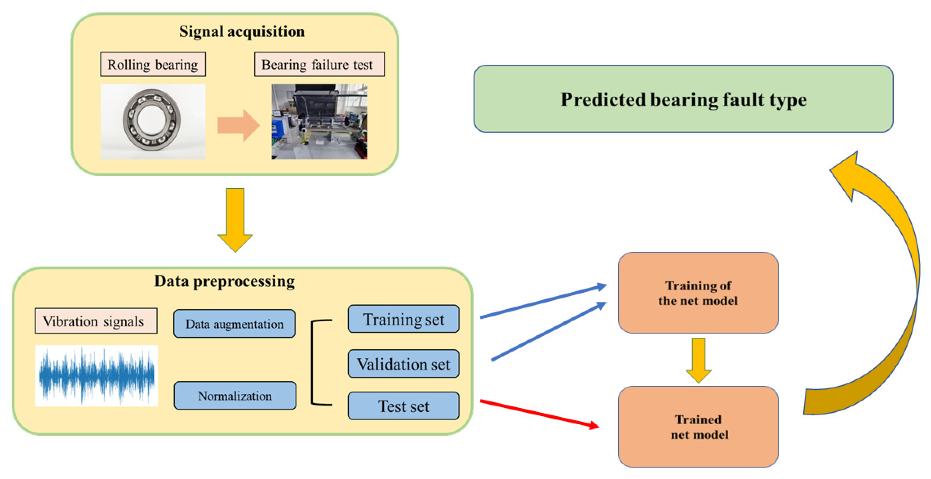
Figure 8 illustrates the overall workflow of the proposed ADCNN-based bearing fault diagnosis framework. It is important to clarify that this workflow consists of two distinct phases: an offline training phase and an online deployment phase.

In the offline training phase, historical vibration signals with labeled bearing conditions (e.g., healthy, inner-ring fault, outer-ring fault, and rolling element fault) are collected from laboratory experiments or previously recorded maintenance data under representative operating conditions. These labeled datasets are used to train the ADCNN model. After the training process converges, the optimized model parameters are fixed. This training procedure is not performed continuously in the practical operating environment but is conducted offline before deployment.

In the online diagnosis phase, only real-time vibration signals from the operating bearing are required. The acquired signals undergo preprocessing steps, including normalization and segmentation, and are then directly input into the pre-trained ADCNN model. The model outputs the predicted bearing condition without any further retraining. Therefore, the practical deployment does not require the simultaneous availability of all fault types in the actual environment.

It should also be noted that while binary fault detection (healthy vs. faulty) may be sufficient for basic maintenance decisions, fine-grained fault-type identification provides additional engineering value. Distinguishing between inner-ring, outer-ring, and rolling element faults supports root-cause analysis, maintenance strategy optimization, and fault progression monitoring, which are essential in predictive maintenance systems.

This clarification ensures that the workflow in Figure 8 reflects a realistic industrial application scenario, where model training and field deployment are clearly separated.

3. Results and Discussion

To verify the effectiveness and progressiveness of the bearing fault diagnosis model in different dataset noise environments, two types of bearing fault datasets are taken as examples to conduct bearing fault diagnosis using the proposed model. The environment required for the fault diagnosis model is as follows: Computers with Win10 operating systems are used in the experiment, and the specific hardware configuration includes an Intel (R) Core (TM) i7-10875H CPU, 16 G RAM and NVDIA RTX2060GPU. The network architecture was developed by Pytorch 1.7.1, and the programming language is Python 3.8.

3.1. Experimental Setup and Hyperparameter Configuration

The network input is a normalized 1D vibration signal segment with a fixed length of 1024 points, formatted as a tensor of size [Batch Size, 1, 1024]. The output is a probability distribution over the fault classes (10 for CWRU, 4 for SJZU). The model was trained using the Adam optimizer with an initial learning rate of 0.001, β1 = 0.9, and β2 = 0.999. Cross-entropy loss was used as the objective function. Training proceeded for a maximum of 100 epochs with a batch size of 64. To prevent overfitting, we employed early stopping (patience = 10 epochs based on validation loss) and L2 weight decay (coefficient = 1 × 10⁻⁴). The learning rate was reduced by a factor of 0.5 if the validation loss plateaued for five consecutive epochs.

To test the model’s robustness under realistic operating conditions, Gaussian white noise of varying intensities (SNR from −5 dB to 5 dB) was added to the original vibration data. This noise simulates the interference commonly encountered in industrial environments, and the model’s ability to perform fault diagnosis under these conditions was thoroughly tested. Sliding window sampling was also employed to ensure signal continuity and avoid class imbalance, further enhancing the training dataset. By using k-fold cross-validation, we ensured that the performance of the fault diagnosis model was not overly dependent on a single dataset split. This helped account for variations in the data, such as signal noise or different fault types, improving the robustness of the model and its ability to generalize to new, unseen data.

For reproducibility, each epoch consisted of ⌈N_train/batch_size⌉ iterations. We also fixed the random seed for data splitting and training. The implementation was based on PyTorch (version specified in the final submission) and executed on the hardware described above. During inference, the trained ADCNN takes an unseen normalized vibration segment of size [Batch Size, 1, 1024] as input and outputs a probability distribution over fault classes via the Softmax layer. The predicted fault category is determined by the maximum-probability class. This inference process supports online diagnosis once the model has been trained offline.

3.2. Data Preprocessing

In this example, both datasets are divided into training sets and test sets in an 8:2 ratio. Data enhancement and standardization processing are performed after the dataset is divided to prevent information leakage from the test set. First, the sample length should be determined based on the parameters known in the experiment, and the number of sampling points for one cycle of bearing operation should be calculated using Formula (18):

$$\begin{array}{c}datalen={\displaystyle \frac{1}{\frac{speed}{60}}}\times freq\end{array}$$

(18)

where $freq$ is the sampling frequency, $speed$ represents the running speed of the bearing, and $datalen$ is the calculated sample length. After calculating the number of sampling points, a sample point greater than this value is selected as the sample length. At the same time, the same number of samples is used for each operating state of the bearings in the training set and the test set to prevent class imbalance in training samples.

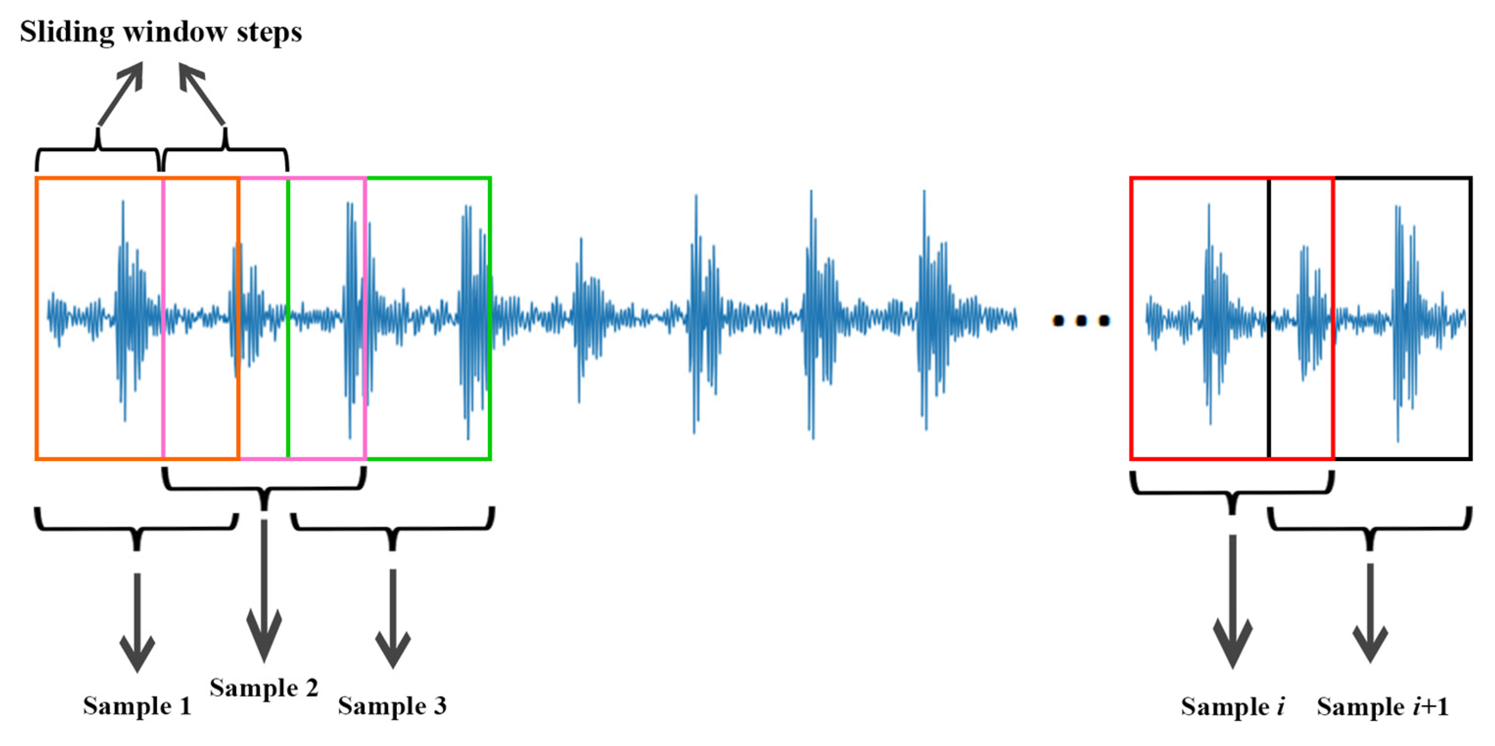
The accuracy of the model largely depends on the number of samples in the training set when the training of a neural network model is conducted. The more samples in the training set, the better the training effect of the model. Therefore, a sliding window overlapping sampling method is used for data enhancement in this experiment, and the process is shown in Figure 9. This method can ensure the continuity of the vibration signals better and complies with the characteristics of signal periodicity. The overlapping sampling formula is expressed as follows:

$$\begin{array}{c} m=\left[{\displaystyle \frac{N-datalen}{datalen}}\right]\end{array}$$

(19)

$$\begin{array}{c} x_i=N\left[i\times S:i\times S+datalen\right]\end{array}$$

(20)

where m is the number of samples, N is the total length of the signal, ${\mathit{x}}_i$ is the i-th sample data point after sampling, $i\in [1,m]$, and S is the length of the sliding window.

The sliding window sampling method is used to generate overlapping samples from the original dataset, effectively increasing the number of samples available for training. It should be emphasized that this approach increases sample redundancy rather than intrinsic data diversity. The primary benefit lies in enabling the model to learn temporal correlations more effectively rather than introducing additional information content. This means that while the model may encounter more examples, the variety of information presented to it remains the same. Therefore, the primary benefit of this method is that it allows the model to learn more about the temporal relationships within the data, particularly when the dataset is small. However, it should not be confused with methods that increase the diversity of training data.

In practical work, rolling bearings are often located in a relatively complicated operating environment, so noises would inevitably interfere with the vibration signals. Gaussian white noise with different intensities is added during data preprocessing to investigate the noise resistance ability of the proposed network model in different noise environments under actual operating conditions. Its intensity is measured by the signal-to-noise ratio (SNR) in decibels. The SNR calculation formula is expressed as follows:

$$\begin{array}{c} SNR=10{log}_{10}{\displaystyle \frac{P_s}{P_n}}\end{array}$$

(21)

where $P_s$ is the effective power of the signal and $P_n$ is the effective power of the noise. The lower the SNR value, the greater the energy of the noise interference and the greater the difficulty in identifying the original signal.

To further illustrate the influence of noise on vibration signals, representative raw signals under clean and noise-contaminated conditions were analyzed. For healthy bearings, the vibration signals exhibit relatively stable periodic patterns with low amplitude variation, whereas faulty bearings (inner-ring, outer-ring, and rolling element faults) show impulsive components and increased signal complexity. As the SNR decreases, these fault-related impulses become progressively masked by noise, leading to blurred time-domain characteristics. This phenomenon is observed consistently in both the CWRU and SJZU datasets and highlights the challenge of extracting discriminative features under severe noise interference.

For the CWRU dataset, labels are categorical indices (0–9), each of which corresponds to a pre-defined bearing health state (e.g., healthy or inner-ring fault with a specific damage size). We trained a single unified multi-class classifier that directly predicts the fault type/severity from raw vibration segments rather than constructing separate datasets for each fault cause. This setting aligns with practical condition monitoring, where a single deployed model is expected to differentiate multiple fault modes and severities.

The predicted fault type refers to the categorical classification output of the ADCNN model. Each category corresponds to a specific bearing condition, including healthy condition, inner-ring fault, outer-ring fault, and rolling element fault, as defined in

Table 3. CWRU data information table.

Running State	Label	Damage Size (mils)	Sample Length	Number of Training-Set Samples	Number of Test-Set Samples
Healthy	0	-	1024	737	25
Inner-ring fault	1	7	1024	737	25
Rolling fault	2	7	1024	737	25
Outer-ring fault	3	7	1024	737	25
Inner-ring fault	4	14	1024	737	25
Rolling fault	5	14	1024	737	25
Outer-ring fault	6	14	1024	737	25
Inner-ring fault	7	21	1024	737	25
Rolling fault	8	21	1024	737	25
Outer-ring fault	9	21	1024	737	25

and Table 6.

Therefore, we did not construct separate datasets for different fault causes; instead, we used one unified multi-class dataset and trained a single classifier to directly identify the fault mode and severity.

3.3. Example 1: Network Model Validation Based on CWRU Dataset

3.3.1. Data Description

For our experiments, we used publicly available data from the Case Western Reserve University (CWRU) Bearing Data Center [39]. This dataset includes data from various bearing fault types, such as inner-ring faults, outer-ring faults, and rolling element faults. The experiment was conducted under a 0 HP load condition with a bearing speed of 1797 RPM. The data were sampled at a frequency of 12 kHz with a sample length of 1024 points. The dataset was divided into training and test sets in an 80:20 ratio, with each fault type having samples with damage sizes of 7 mil, 14 mil, and 21 mil. Given that the test set comprises less than 5% of the total data, k-fold cross-validation (with k = 5) was employed to mitigate the risk of evaluating the model based on a small and potentially unrepresentative test set. This technique ensures that each sample has a chance to be used as a test set, providing a more robust and generalized estimate of the model’s performance. The CWRU dataset was collected using a deep-groove ball-bearing test rig.

The bearing type used in the experiment was SKF 6205-2RS JEM, with the following specifications: Inner diameter: 25 mm; Outer diameter: 52 mm; Width: 15 mm.

Faults were artificially introduced using electro-discharge machining (EDM), which produced localized defects on the inner ring, outer ring, and rolling elements. Fault diameters were 0.007 inches (0.178 mm), 0.014 inches (0.356 mm), and 0.021 inches (0.533 mm).

The motor load conditions correspond to different torque levels applied to the motor shaft. The 0 HP condition corresponds to a no-load motor condition with a nominal rotational speed of 1797 RPM.

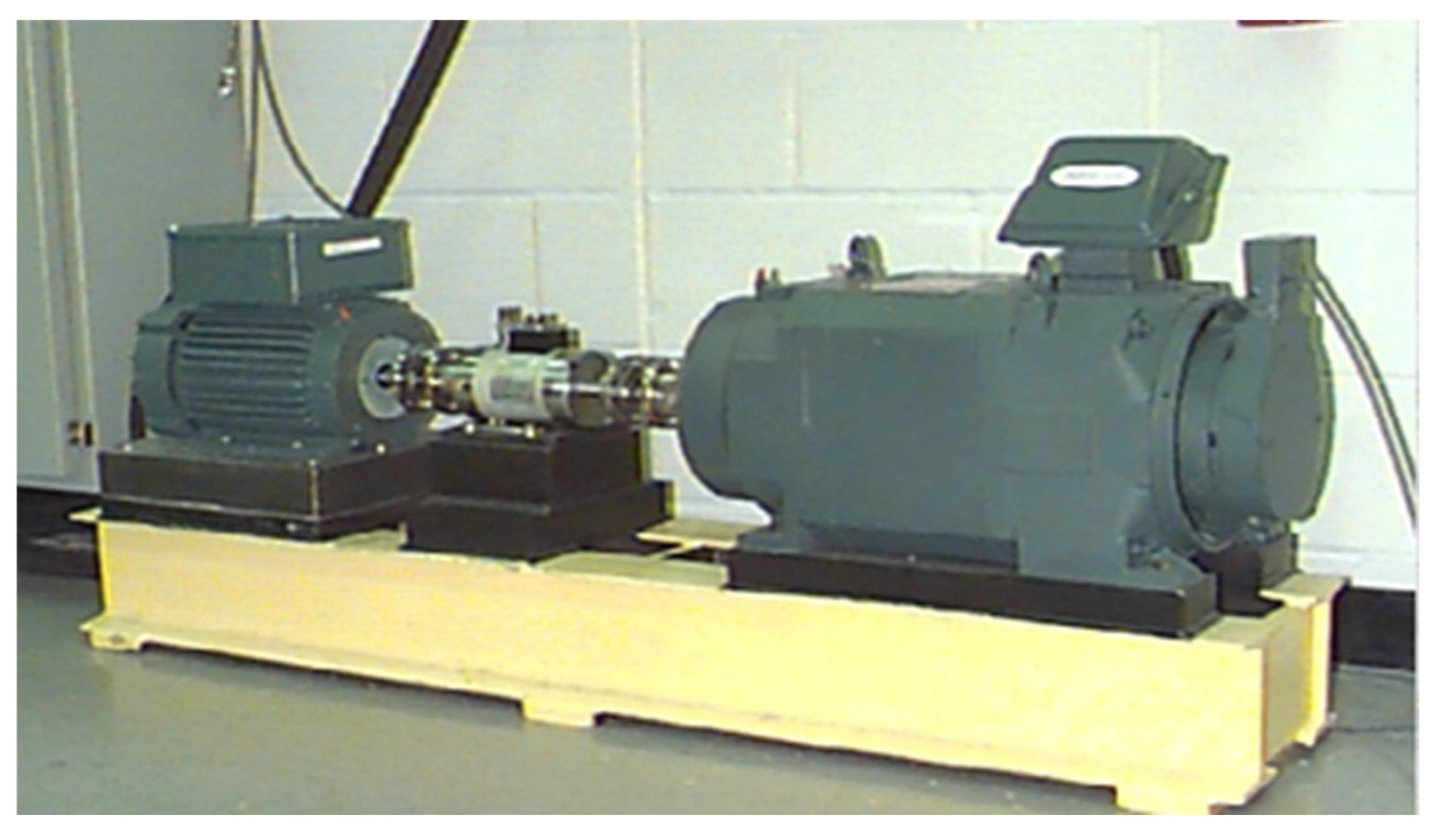
The dataset used in this experimental validation comprises open-source data released by the CWRU Bearing Data Center. As shown in Figure 10, the test bench consists of four parts: a drive motor, a torque sensor, a power tester and a console. In the bearing experiment, vibration signals were recorded under four load conditions (0 HP, 1 HP, 2 HP, and 3 HP). The 0 HP load condition refers to a no external mechanical load applied to the motor shaft, while the bearing rotates at its nominal operating speed. This condition is commonly used as a baseline operating condition in the CWRU dataset.

These four loads correspond to different bearing speeds. In this paper, the signals under the 0 HP operating condition were selected for validation, the corresponding speed was 1797 r/min, and the sampling frequency for the experiment was 12 KHz. The data includes ten states of normal bearings, three types of bearing outer-ring faults, three types of bearing inner-ring faults, and three types of bearing roller faults. The corresponding damage sizes for the three types of bearing failures are 7 mil, 14 mil, and 21 mil.

Based on the above, it is calculated that at least about 400 sampling points are passed during one revolution of the bearing. The final sample length was determined to be 1024 to better extract the feature information. In addition, a sliding window size of 128 was selected for the data enhancement operation. The details of the data samples after dataset enhancement are shown in the Table 3.

The labels (0 to 9 for CWRU) are categorical, each representing a specific, pre-defined health state of the bearing (e.g., healthy or inner-ring fault of 0.007 inches). This comprehensive dataset encompassing multiple fault types and severities is essential for the training of a unified diagnostic model capable of directly identifying a wide range of potential failures from raw vibration signals, which aligns with the practical need for versatile condition monitoring systems in industry.

To verify the effectiveness and progressiveness of the method proposed in this paper for fault diagnosis in different noise environments, we added white Gaussian noise with an SNR of −5 dB to 5 dB to the original dataset to test the noise resistance performance and robustness of the model.

During data preprocessing, Gaussian white noise of varying intensities, with a Signal-to-Noise Ratio (SNR) ranging from −5 dB to +5 dB, was added to the original vibration data. This range simulates the noise interference typically encountered in industrial environments. Specifically, an extreme noise level of −5 dB was chosen to test the model’s performance under challenging conditions.

3.3.2. Experimental Results and Analysis

We performed experiments using the publicly available dataset from the CWRU Bearing Data Center. The data was collected under a 0 HP load condition at a speed of 1797 RPM with a sampling frequency of 12 kHz. In the preprocessing stage, we applied a sliding window technique for data augmentation and standardized the data. The dataset was split into training and testing sets in an 80:20 ratio, and each sample was 1024 points long. The fault types included in the dataset are inner-ring faults, outer-ring faults, and rolling element faults, with damage sizes of 7 mil, 14 mil, and 21 mil, respectively. The dataset, which includes various fault types, such as inner-ring faults, outer-ring faults, and rolling element faults, was split into training and test sets in an 80:20 ratio to ensure balance. For data augmentation, the sliding window method was applied during preprocessing, using a window size of 128 samples with 50% overlap. Furthermore, each combination of fault type and damage size was represented with multiple samples to increase dataset variability and robustness. The fault types included in the dataset are: inner-ring fault (7 mil, 14 mil, and 21 mil), outer-ring fault (7 mil, 14 mil, and 21 mil), and rolling element fault (7 mil, 14 mil, and 21 mil).

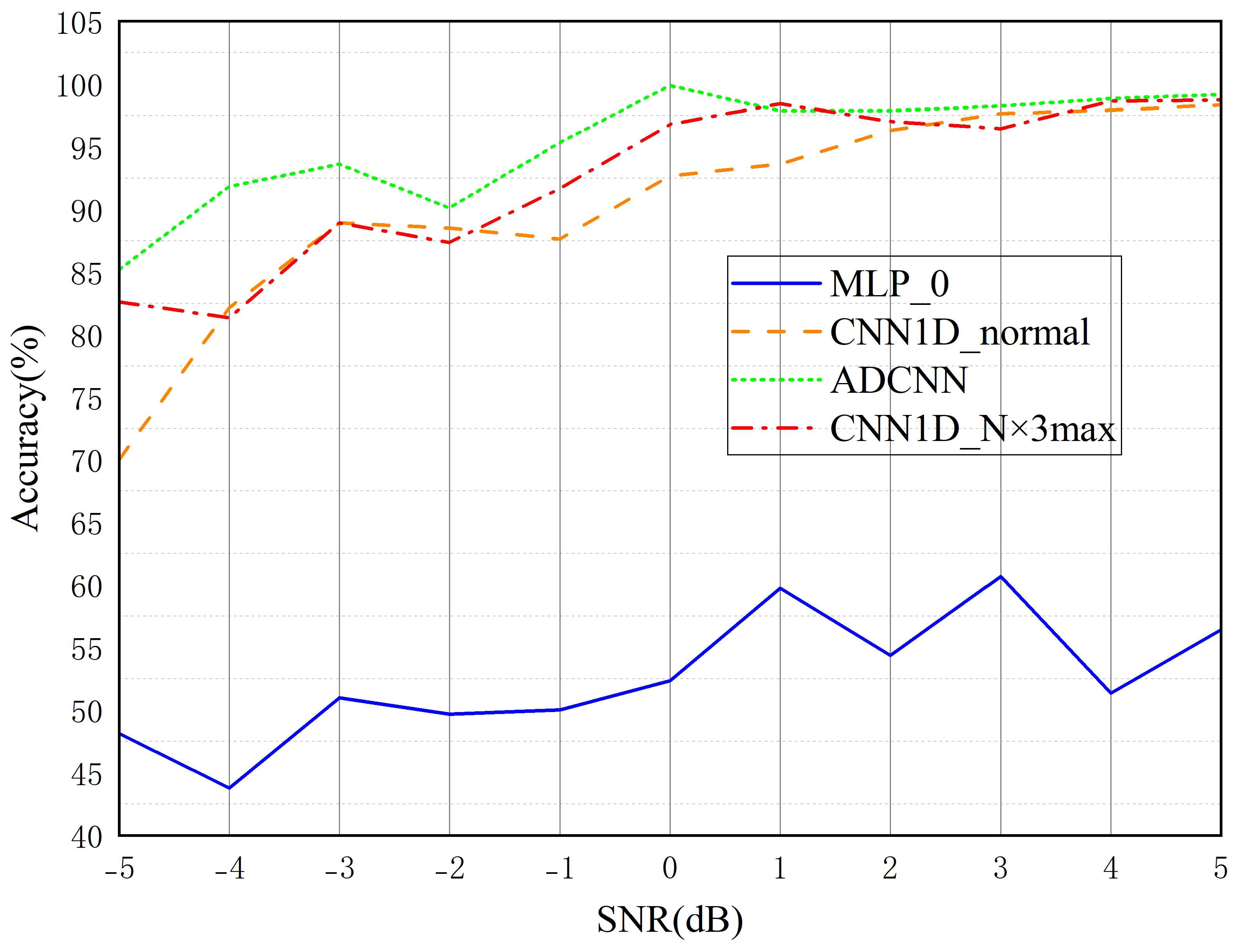
To verify the model, the diagnosis results of the ADCNN model proposed in this paper are compared with those of several traditional network models. Traditional models include the excellent lightweight MLP_0 model, conventional CNN model, and CNN1D_N×3Max model with good noise resistance.

Table 4. Sizes and prediction times of different models.

Model	Model Size (KB)	Prediction Time (ms)
ADCNN	54.23	321
MLP_0	2733.79	135
CNN1D_normal	556.79	295
CNN1D_N×3max	4713.22	430

shows the sizes and prediction speeds of different models.

Table 5. Table of noise resistance performance of different models on the CWRU dataset.

Model	SNR (dB)
	−5	−4	−3	−2	−1	0	1	2	3	4	5
ADCNN	81.1	86.4	90.32	94.36	94.08	97.64	99.44	99.52	98.2	100	99.8
MLP_0	59.04	67.88	68.28	74.32	77.6	83.52	82.24	86.32	86.04	84.88	87.6
CNN1D_normal	54.48	60.24	72.32	81.76	79.16	86.96	89.36	90.92	92.8	97.48	99.2
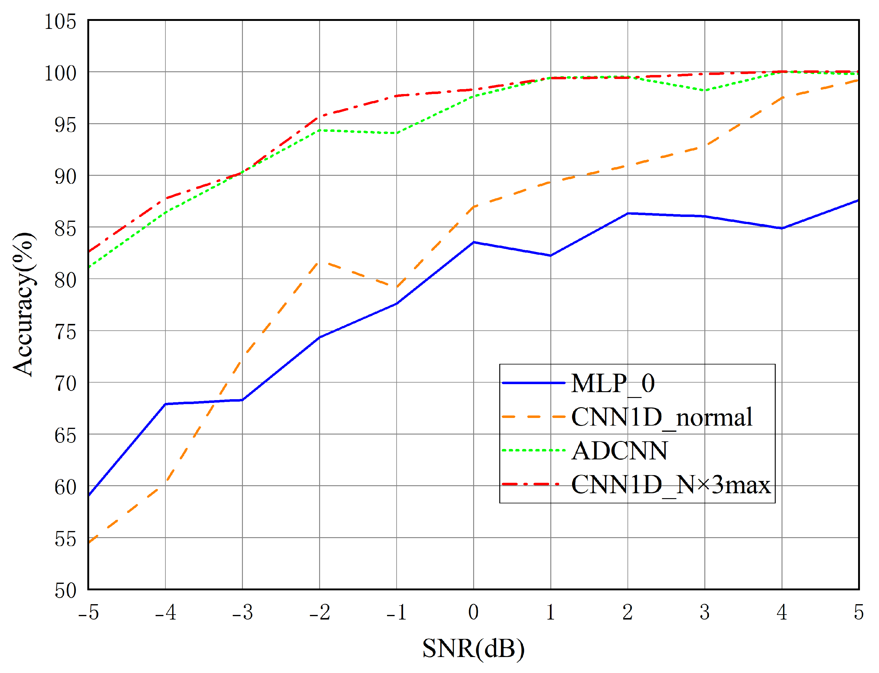
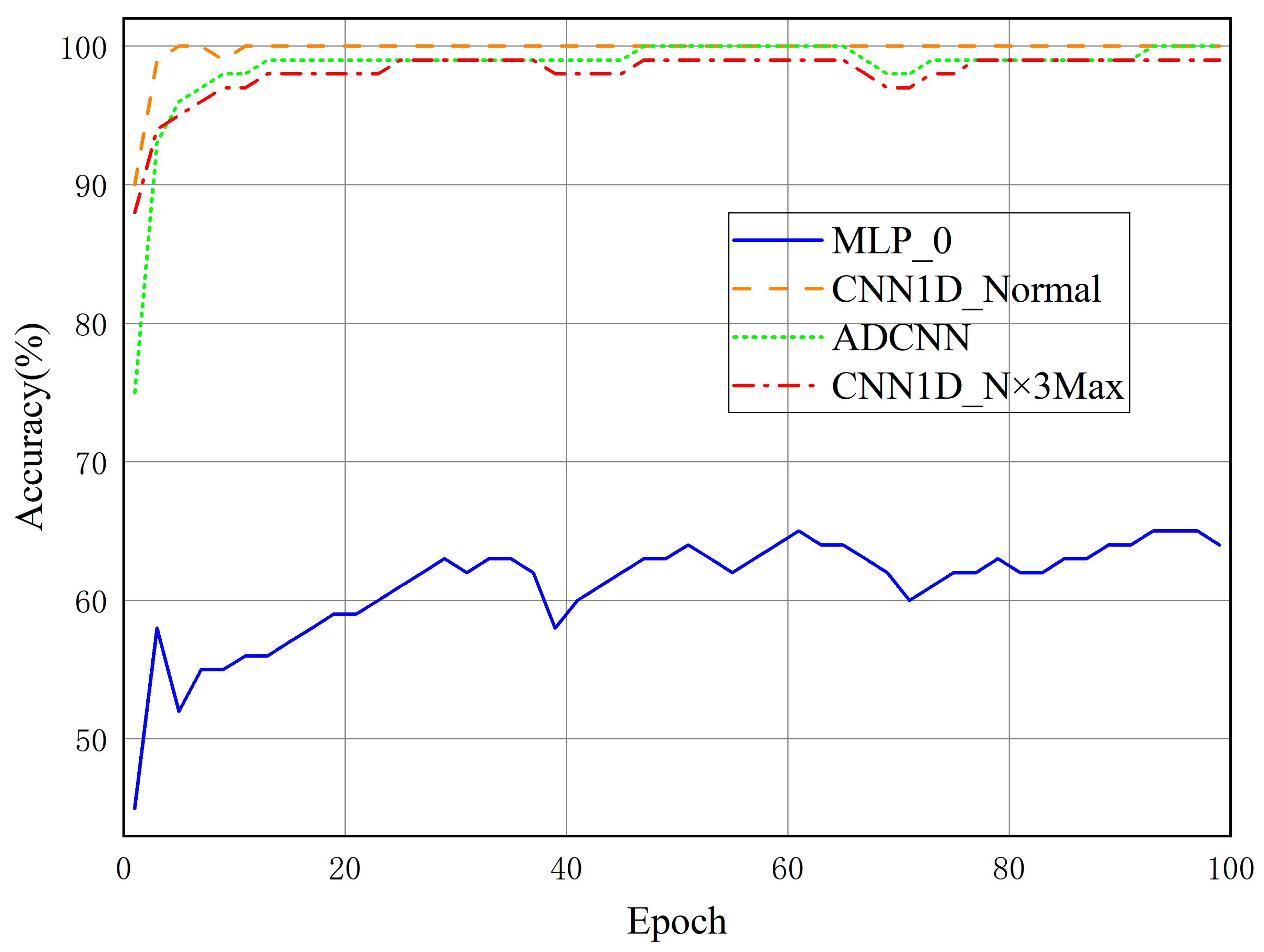
CNN1D_N×3max	82.6	87.76	90.24	95.68	97.68	98.28	99.4	99.44	99.8	100	100

and Figure 12 present comparisons of the diagnostic accuracies of different models, and Figure 13 reveals the model accuracy under different numbers of epochs.

As seen in Table 5 and Figure 11 and Figure 12, ADCNN consistently outperforms traditional models, especially under low-SNR conditions. With a noise resistance rate exceeding 99% at higher SNR levels (0 dB and above), ADCNN’s performance in feature extraction and fault classification significantly surpasses that of the MLP_0 model and conventional CNN architectures. This confirms the superiority of ADCNN in handling noisy industrial data.

Table 5 and Figure 12 indicate that the accuracy is low for MLP_0 and CNN1D_Normal in areas with high noise interference (SNR = −5 dB~−1 dB). The accuracy of fault diagnosis is lower than 60%, especially when SNR = −5 dB. The accuracy is lower than 80% when SNR = −1 dB, which indicates that MLP_0 and CNN1D_Normal have poor noise resistance. ADCNN and CNN1D_N×3Max have similar effects, with an accuracy of more than 80% when SNR = −5 dB. The fault diagnosis accuracy of ADCNN and CNN1D_N×3Max is around 95% when SNR = −1 dB. ADCNN and CNN1D_N×3Max have the advantage of noise resistance performance in areas with lower noise interference (SNR = 0 dB~5 dB), with an accuracy of around 99%.

To further analyze the potential overfitting behavior of the proposed ADCNN model, classification accuracy under different numbers of training epochs was investigated. As shown in Figure 12, when the number of training epochs is lower than 40, both training and test accuracy increase steadily, indicating effective learning features. However, when the number of epochs exceeds approximately 50, the training accuracy continues to improve, while the test accuracy shows noticeable fluctuations or slight degradation. This phenomenon suggests a potential tendency toward memorizing training patterns rather than further improving generalization performance. Further increasing the number of training epochs does not lead to additional performance improvement and may introduce a potential risk of overfitting.

Based on this observation, an appropriate training epoch range was selected to balance model convergence and generalization performance. In this study, the optimal number of training epochs for ADCNN was empirically determined to be within the range of 40 to 50, where the model achieves high diagnostic accuracy while maintaining stable performance on the test set.

According to Table 4, from the perspective of model size and prediction time, the parameter count of ADCNN is only 1.15% that of CNN1D_N×3Max, requiring a shorter training time. Combining noise immunity and model size, ADCNN outperforms other networks, highlighting its advantages in fault diagnosis tasks. Figure 13 shows that the network accuracy during training will fluctuate with a continuous increase in the number of training epochs, indicating that attention should be paid to the selection of the number of epochs during ADCNN network training to enhance the network stability.

Although CNN1D_N×3Max achieves comparable accuracy to ADCNN under certain SNR conditions, ADCNN demonstrates clear advantages in terms of model compactness and computational efficiency. Specifically, ADCNN requires significantly less memory and exhibits a lower prediction time, as shown in Table 4. This trade-off between accuracy and efficiency highlights the superiority of ADCNN for practical industrial deployment, where both noise robustness and resource constraints must be considered simultaneously.

3.4. Example 2: Validation of the Designed Test Dataset

3.4.1. Data Description

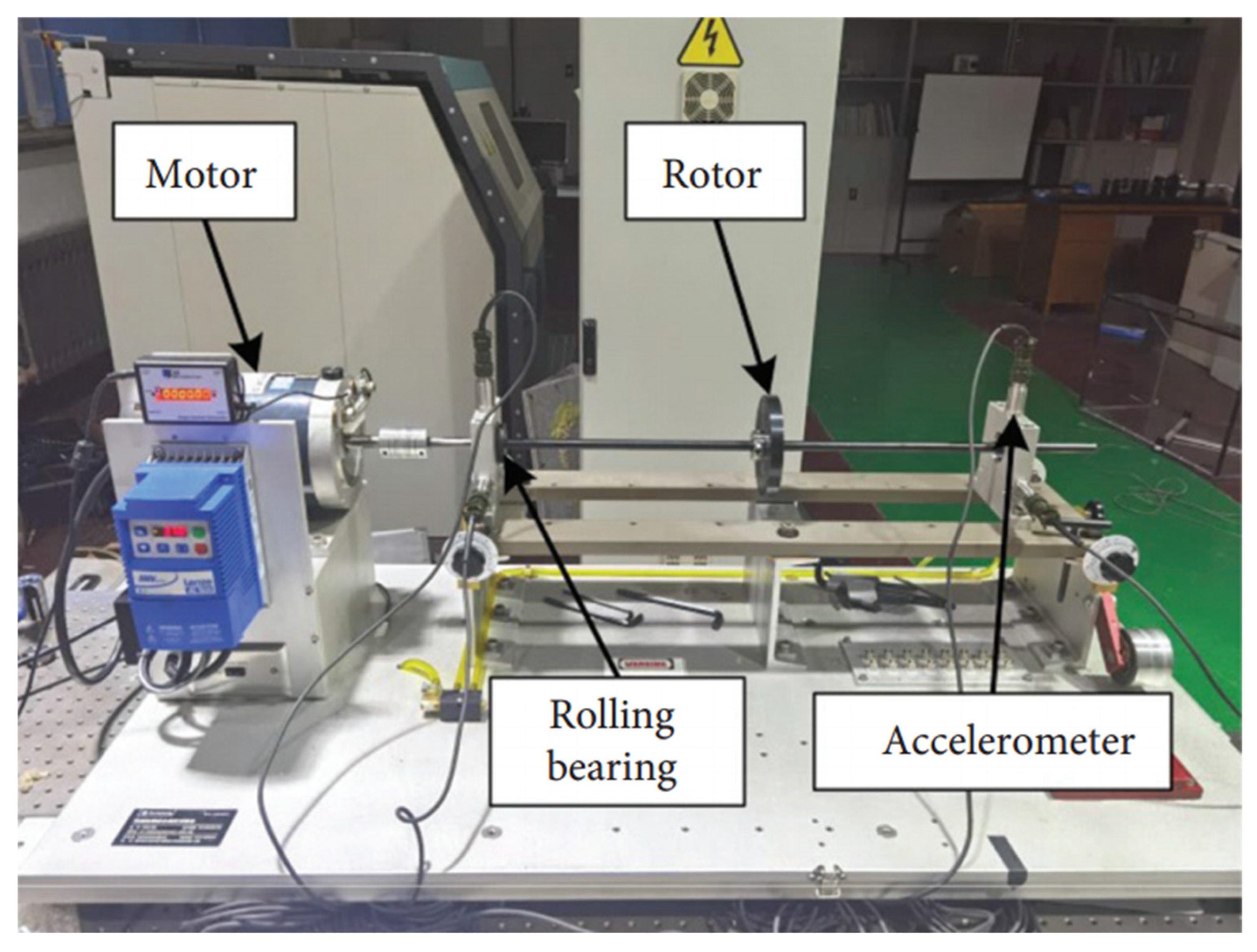
This part of experimental validation data was obtained from the bearing failure test bench of Shenyang Jianzhu University (SJZU). The structure of the test bench is shown in Figure 13. The entire test bench consists of three parts: a drive motor, a rotor, and an acceleration tester. The bearing experiment was conducted under a load condition of 0 HP, with a rotation frequency of 20 HZ and a sampling frequency of 16,384 HZ. The data includes four states: normal bearing, bearing outer-ring fault, bearing inner-ring fault, and bearing roller fault. The bearing used in the SJZU test bench is a deep-groove ball bearing (model: MB ER-8K, Spectra Quest Inc., Richmond, VA, USA). The bearing contains eight rolling elements, with a rolling-element diameter of 0.3125 inch and a pitch diameter of 1.319 inch. The contact angle is 0°. These detailed bearing parameters are provided to ensure the full reproducibility of the experimental conditions. Faults were introduced artificially using controlled machining to simulate realistic defect conditions.

The labels (0 to 3 for SJZU) are categorical, each representing a specific, pre-defined health state of the bearing (e.g., Healthy, inner-ring fault of 0.007 inches). This comprehensive dataset encompassing multiple fault types and severities is essential for the training of a unified diagnostic model capable of directly identifying a wide range of potential failures from raw vibration signals, which aligns with the practical need for versatile condition monitoring systems in industry.

Like example 1, it is calculated that the bearing passes through at least about 820 sampling points during one revolution, and the sample length was also determined to be 1024. A sliding window size of 128 was selected for the data enhancement operation. The data details are shown in the table below (

Table 6. SJZU data information table.

Running State	Label	Sample Length	Number of Training-Set Samples	Number of Test-Set Samples
Healthy	0	1024	448	15
Inner-ring fault	1	1024	448	15
Rolling fault	2	1024	448	15
Outer-ring fault	3	1024	448	15

).

To verify the universality of the proposed method in terms of noise resistance performance, we adopted the same scheme as the original dataset in example 1 and added white Gaussian noise with an SNR of −5 dB to 5 dB.

3.4.2. Experimental Results and Analysis

The designed test datasets are used as examples in this section, and the MLP_0 model, conventional CNN model, CNN1D_N×3Max model and ADCNN model are used for fault diagnosis.

Table 7. Sizes and prediction times of different models on SJZU dataset.

Model	Model Size (KB)	Prediction Time (ms)
ADCNN	48.76	293
MLP_0	2136.87	108
CNN1D_normal	497.51	241
CNN1D_N×3max	4473.37	407

shows the model sizes and operation time comparisons of different network models for the test dataset.

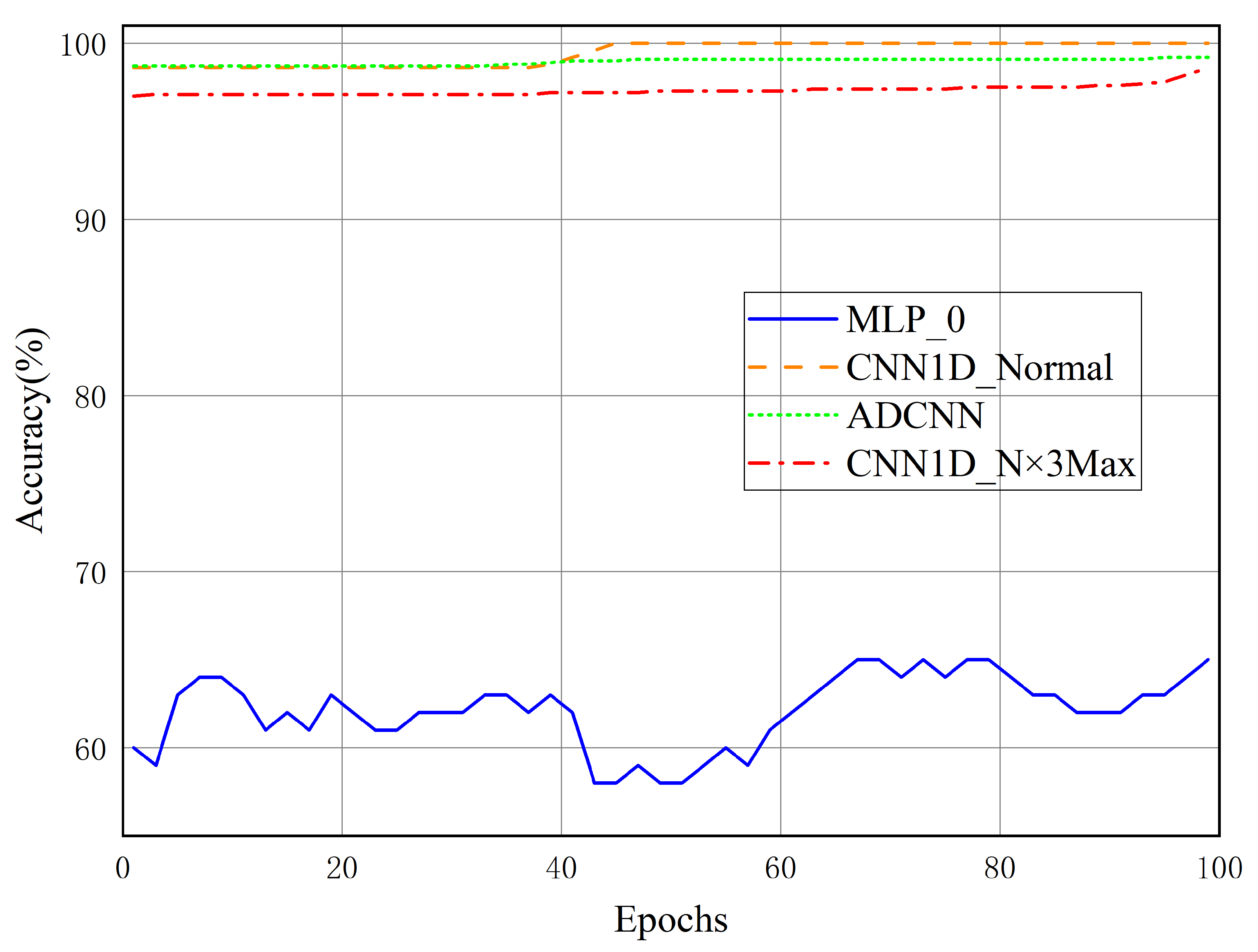
Table 7 indicates that the scale of the ADCNN model is smaller than that of other networks.

Table 8. Table of noise resistance performance of different models on SJZU datasets.

Model	SNR (dB)
	−5	−4	−3	−2	−1	0	1	2	3	4	5
ADCNN	85.2	91.83	93.62	90.12	95.34	99.87	97.86	97.53	98.25	98.84	99.16
MLP_0	48.13	43.78	50.98	49.67	50.02	52.34	59.76	54.37	60.67	51.35	56.41
CNN1D_normal	70	82.16	88.93	88.5	87.64	92.68	93.61	96.31	97.64	97.91	98.32
CNN1D_N×3max	82.62	81.35	88.92	87.35	91.68	96.78	98.43	97.02	96.44	98.63	98.72

and Figure 14 show the obtained fault diagnosis accuracy of each network model on the dataset.

Table 8 and Figure 14 show that ADCNN performs well in the validation of design test datasets. Under the condition of high noise interference (SNR = −5 dB~−1 dB), its accuracy is still higher than that of other networks. The accuracy can be maintained within a range of 85–95%. The accuracy of conventional CNN models is below 90%. As a neural network with good noise resistance, the accuracy of CNN1D_N×3Max is over 90% only when the SNR is −1 dB, and the accuracy of MLP_0 within this range can only reach about 50%. In the case of limited noise interference (SNR = 0 dB~5 dB), the accuracy of ADCNN can reach up to 99.87%. The above result further proves that ADCNN achieves good noise resistance performance.

As shown in Table 7, the model size of ADCNN is 48.76 KB, making it much smaller than CNN1D_Normal, the second smallest model. Although slightly larger than MLP_0 in runtime, ADCNN is still better than other networks in terms of comprehensive noise resistance performance and recognition accuracy. Figure 15 indicates that in the SJZU dataset, the optimal number of training epochs for the ADCNN network is within the range of 40–50. Beyond this number, the effect will not be as good as CNN1D_N×3Max. This indicates that when using this dataset for network experiments, excessive training times can lead to overfitting problems, affecting the accuracy of the network. It further indicates that attention should be paid to the setting of the number of epochs during network training.

Accuracy is adopted as the primary evaluation metric in this study, as the datasets are balanced across fault categories. Under such conditions, accuracy provides a reliable indicator of overall classification performance. Nevertheless, metrics such as precision, recall, and F1 score are also important for evaluating false-positive and false-negative rates, particularly in imbalanced scenarios. A more comprehensive multi-metric evaluation will be considered in future work to further assess the diagnostic reliability of the proposed method.

4. Conclusions

This study proposes an Ascending-Dimensional Convolutional Neural Network (ADCNN) for rolling bearing fault diagnosis under noisy conditions. The key innovations of this work include the introduction of large convolutional kernels for enhanced noise robustness, an ascending-dimensional feature construction strategy based on weight sharing, and a reduced linear transformation layer (RLTL) to achieve a lightweight architecture. Experimental results on two datasets demonstrate that ADCNN achieves a favorable balance between diagnostic accuracy, noise resistance, and computational efficiency. Based on two bearing datasets, the performance of the proposed network model was verified, and the following conclusions can be reached:

(1)

Compared with traditional fault diagnosis models, ADCNN achieves higher efficiency in feature extraction and fault diagnosis based on complicated feature signals.

(2)

ADCNN can ensure the accuracy of fault diagnosis with fewer parameters. Compared with traditional CNN and machine learning methods, ADCNN has lower requirements on working hardware and has higher accuracy.

(3)

ADCNN achieves good diagnostic performance in performance tests on different data sets, indicating that the network has good universality under different operating conditions.

However, experimental results indicate that when the number of training epochs exceeds approximately 50, the diagnostic accuracy on the test set no longer improves and may even slightly decrease, while the training accuracy continues to increase. This behavior suggests the risk of overfitting, highlighting the importance of selecting an appropriate training duration for the proposed ADCNN model, and excessive training times would affect the accuracy of the network model. In the future, we will further improve the ADCNN network to address this phenomenon. In future work, additional strategies such as early stopping, data augmentation and optimization, and explicit regularization techniques will be investigated to further enhance the generalization ability of the model.

References

1. Zhang, Y.; Xing, K.; Bai, R.; Sun, D.; Meng, Z. An enhanced convolutional neural network for bearing fault diagnosis based on time–frequency image. Measurement 2020, 157, 107667. [Google Scholar] [CrossRef]
2. Randall, R.B.; Antoni, J. Rolling element bearing diagnostics—A tutorial. Mech. Syst. Signal Process. 2011, 25, 485–520. [Google Scholar] [CrossRef]
3. Cui, L.; Jin, Z.; Huang, J.; Wang, H. Fault Severity Classification and Size Estimation for Ball Bearings Based on Vibration Mechanism. IEEE Access 2019, 7, 56107–56116. [Google Scholar] [CrossRef]
4. Georgoulas, G.; Loutas, T.; Stylios, C.D.; Kostopoulos, V. Bearing fault detection based on hybrid ensemble detector and empirical mode decomposition. Mech. Syst. Signal Process. 2013, 41, 510–525. [Google Scholar] [CrossRef]
5. Jardine, A.K.S.; Lin, D.; Banjevic, D. A review on machinery diagnostics and prognostics implementing condition-based maintenance. Mech. Syst. Signal Process. 2006, 20, 1483–1510. [Google Scholar] [CrossRef]
6. Li, Y.; Xu, M.; Zhao, H.; Huang, W. Hierarchical fuzzy entropy and improved support vector machine based binary tree approach for rolling bearing fault diagnosis. Mech. Mach. Theory 2016, 98, 114–132. [Google Scholar] [CrossRef]
7. Shao, H.; Jiang, H.; Zhao, H.; Wang, F. A novel deep autoencoder feature learning method for rotating machinery fault diagnosis. Mech. Syst. Signal Process. 2017, 95, 187–204. [Google Scholar] [CrossRef]
8. Yao, D.; Liu, H.; Yang, J.; Li, X. A lightweight neural network with strong robustness for bearing fault diagnosis. Measurement 2020, 159, 107756. [Google Scholar] [CrossRef]
9. Wang, D.; Zhao, Y.; Yi, C.; Tsui, K.-L.; Lin, J. Sparsity guided empirical wavelet transform for fault diagnosis of rolling element bearings. Mech. Syst. Signal Process. 2018, 101, 292–308. [Google Scholar] [CrossRef]
10. Kiral, Z.; Karagülle, H. Simulation and analysis of vibration signals generated by rolling element bearing with defects. Tribol. Int. 2003, 36, 667–678. [Google Scholar] [CrossRef]
11. Jiang, X.; Shen, C.; Shi, J.; Zhu, Z. Initial center frequency-guided VMD for fault diagnosis of rotating machines. J. Sound Vib. 2018, 435, 36–55. [Google Scholar] [CrossRef]
12. Hu, Z.-X.; Wang, Y.; Ge, M.-F.; Liu, J. Data-driven fault diagnosis method based on compressed sensing and improved multiscale network. IEEE Trans. Ind. Electron. 2019, 67, 3216–3225. [Google Scholar] [CrossRef]
13. Yang, L.; Sun, Y.; Sun, R.; Gao, L.; Chen, X. Analytical Modeling and Mechanism Analysis of Time-Varying Excitation for Surface Defects in Rolling Element Bearings. J. Dyn. Monit. Diagn. 2023, 2, 89–101. [Google Scholar]
14. Melluso, F.; Spirto, M.; Nicolella, A.; Malfi, P.; Tordela, C.; Cosenza, C.; Niola, V. Torque fault signal extraction in hybrid electric powertrains through a wavelet-supported processing of residuals. Mech. Syst. Signal Process. 2026, 242, 113652. [Google Scholar] [CrossRef]
15. Padovese, L. Comparison between probabilistic and multilayer perceptron neural networks for rolling bearing fault classification. Int. J. Model. Simul. 2002, 22, 97–103. [Google Scholar] [CrossRef]
16. Samanta, B.; Al-Balushi, K.R.; Al-Araimi, S.A. Artificial neural networks and genetic algorithm for bearing fault detection. Soft Comput. 2006, 10, 264–271. [Google Scholar] [CrossRef]
17. Yang, Y.; Zheng, H.; Li, Y.; Xu, M.; Chen, Y. A fault diagnosis scheme for rotating machinery using hierarchical symbolic analysis and convolutional neural network. ISA Trans. 2019, 91, 235–252. [Google Scholar] [CrossRef]
18. Zhang, R.; Tao, H.; Wu, L.; Guan, Y. Transfer learning with neural networks for bearing fault diagnosis in changing working conditions. IEEE Access 2017, 5, 14347–14357. [Google Scholar] [CrossRef]
19. Yang, B.; Lei, Y.; Jia, F.; Xing, S. An intelligent fault diagnosis approach based on transfer learning from laboratory bearings to locomotive bearings. Mech. Syst. Signal Process. 2019, 122, 692–706. [Google Scholar] [CrossRef]
20. Zhang, W.; Li, X.; Ding, Q. Deep residual learning-based fault diagnosis method for rotating machinery. ISA Trans. 2019, 95, 295–305. [Google Scholar] [CrossRef] [PubMed]
21. Ma, S.; Chu, F.; Han, Q. Deep residual learning with demodulated time-frequency features for fault diagnosis of planetary gearbox under nonstationary running conditions. Mech. Syst. Signal Process. 2019, 127, 190–201. [Google Scholar] [CrossRef]
22. Goodfellow, I.J.; Pouget-Abadie, J.; Mirza, M.; Xu, B.; Warde-Farley, D.; Ozair, S.; Courville, A.; Bengio, Y. Generative adversarial networks. Commun. ACM 2020, 63, 139–144. [Google Scholar] [CrossRef]
23. Hinton, G.E.; Osindero, S.; Teh, Y.-W. A fast learning algorithm for deep belief nets. Neural Comput. 2006, 18, 1527–1554. [Google Scholar] [CrossRef] [PubMed]
24. LeCun, Y.; Bottou, L.; Bengio, Y.; Haffner, P. Gradient-based learning applied to document recognition. Proc. IEEE 1998, 86, 2278–2324. [Google Scholar] [CrossRef]
25. Krizhevsky, A.; Sutskever, I.; Hinton, G.E. Imagenet classification with deep convolutional neural networks. Commun. ACM 2017, 60, 84–90. [Google Scholar] [CrossRef]
26. Mikolov, T.; Karafiát, M.; Burget, L.; Cernocký, J.; Khudanpur, S. Recurrent neural network-based language model. In Proceedings of the INTERSPEECH 2010, 11th Annual Conference of the International Speech Communication Association, Chiba, Japan, 26–30 September 2010; pp. 1045–1048. [Google Scholar]
27. Greenspan, H.; Van Ginneken, B.; Summers, R.M. Guest editorial deep learning in medical imaging: Overview and future promise of an exciting new technique. IEEE Trans. Med. Imaging 2016, 35, 1153–1159. [Google Scholar] [CrossRef]
28. Chen, C.; Seff, A.; Kornhauser, A.; Xiao, J. Deepdriving: Learning affordance for direct perception in autonomous driving. In Proceedings of the IEEE International Conference on Computer Vision, Santiago, Chile, 7–13 December 2015; IEEE Computer Society: Washington, DC, USA, 2015; pp. 2722–2730. [Google Scholar]
29. Janssens, O.; Slavkovikj, V.; Vervisch, B.; Stockman, K.; Loccufier, M.; Verstockt, S.; Van de Walle, R.; Van Hoecke, S. Convolutional neural network-based fault detection for rotating machinery. J. Sound Vib. 2016, 377, 331–345. [Google Scholar] [CrossRef]
30. Xue, F.; Zhang, W.; Xue, F.; Li, D.; Xie, S.; Fleischer, J. A novel intelligent fault diagnosis method of rolling bearing based on two-stream feature fusion convolutional neural network. Measurement 2021, 176, 109226. [Google Scholar] [CrossRef]
31. Zhao, B.; Zhang, X.; Zhan, Z.; Wu, Q. A robust construction of normalized CNN for online intelligent condition monitoring of rolling bearings considering variable working conditions and sources. Measurement 2021, 174, 108973. [Google Scholar] [CrossRef]
32. Iandola, F.N.; Han, S.; Moskewicz, M.W.; Ashraf, K.; Dally, W.J.; Keutzer, K. SqueezeNet: AlexNet-level accuracy with 50x fewer parameters and <0.5 MB model size. arXiv 2016, arXiv:1602.07360. [Google Scholar]
33. Chollet, F. Xception: Deep learning with depthwise separable convolutions. In Proceedings of the IEEE Conference on Computer Vision and Pattern Recognition, Honolulu, HI, USA, 21–26 July 2017; pp. 1251–1258. [Google Scholar]
34. Howard, A.G.; Zhu, M.; Chen, B.; Kalenichenko, D.; Wang, W.; Weyand, T.; Andreetto, M.; Adam, H. Mobilenets: Efficient convolutional neural networks for mobile vision applications. arXiv 2017, arXiv:1704.04861. [Google Scholar] [CrossRef]
35. Zhang, X.; Zhou, X.; Lin, M.; Sun, J. Shufflenet: An extremely efficient convolutional neural network for mobile devices. In Proceedings of the IEEE Conference on Computer Vision and Pattern Recognition, Salt Lake City, UT, USA, 18–23 June 2018; pp. 6848–6856. [Google Scholar]
36. Ma, S.; Liu, W.; Cai, W.; Shang, Z.; Liu, G. Lightweight deep residual CNN for fault diagnosis of rotating machinery based on depthwise separable convolutions. IEEE Access 2019, 7, 57023–57036. [Google Scholar] [CrossRef]
37. Li, X.; Li, J.; Zhao, C.; Qu, Y.; He, D. Gear pitting fault diagnosis with mixed operating conditions based on adaptive 1D separable convolution with residual connection. Mech. Syst. Signal Process. 2020, 142, 106740. [Google Scholar] [CrossRef]
38. Zhang, W.; Peng, G.; Li, C.; Chen, Y.; Zhang, Z. A New Deep Learning Model for Fault Diagnosis with Good Anti-Noise and Domain Adaptation Ability on Raw Vibration Signals. Sensors 2017, 17, 425. [Google Scholar] [CrossRef]
39. Smith, W.A.; Randall, R.B. Rolling element bearing diagnostics using the Case Western Reserve University data: A benchmark study. Mech. Syst. Signal Process. 2015, 64, 100–131. [Google Scholar] [CrossRef]
Figure 1. Schematic diagram of convolution: (a) standard convolution; (b) grouping convolution.
Machines 14 00302 g001
Figure 2. Convolutional channel information allocation method: (a) conventional channel information transmission; (b) decentralized channel information transmission; (c) channel shuffle information transmission.
Machines 14 00302 g002
Figure 3. Step diagram of the channel shuffle operation.
Machines 14 00302 g003
Figure 4. Schematic diagram of full-connection network weights. The symbol ‘*’ denotes the convolution operation in the schematic representation.
Machines 14 00302 g004
Figure 5. Schematic diagram of weight sharing. The symbol ‘*’ denotes the convolution operation in the schematic representation. The green circles represent input feature nodes. The blue circles represent intermediate feature map nodes. The yellow region indicates the receptive field of the convolution kernel (3 × 1). The orange circles denote output feature nodes. The black lines represent weighted connections (W1, W2, W3), and the arrow indicates the data flow direction.
Machines 14 00302 g005
Figure 6. Schematic diagram of channel dimension promotion. ①–③ denote three representative sliding-window segments extracted from the multi-channel vibration signal.
Machines 14 00302 g006
Figure 7. Schematic diagram of equivalent transformation of the full connection layer.
Machines 14 00302 g007
Figure 8. Flow chart of the proposed model.
Machines 14 00302 g008
Figure 9. Working process of sliding window.
Machines 14 00302 g009
Figure 10. CWRU test bench.
Machines 14 00302 g010
Figure 11. Accuracy diagram of different models on CWRU dataset.
Machines 14 00302 g011
Figure 12. Model accuracy diagram corresponding to different numbers of training epochs.
Machines 14 00302 g012
Figure 13. Bearing test bench at Shenyang Jianzhu University (SJZU).
Machines 14 00302 g013
Figure 14. Accuracy of different models on SJZU datasets.
Machines 14 00302 g014
Figure 15. Model accuracy corresponding to different numbers of epochs.
Machines 14 00302 g015