Smart Predictive Maintenance: A TCN-Based System for Early Fault Detection in Industrial Machinery

Abstract

Modern factories still struggle with unexpected machine failures because traditional maintenance systems depend on fixed rules and threshold-based alerts. These older approaches often overlook subtle or complex patterns in multimodal sensor data, causing them to miss early signs of wear and leading to late or incorrect maintenance decisions. As a result, production can slow down, costs increase and equipment reliability suffers. To address this challenge, this study introduces a smart and interpretable fault diagnosis and predictive maintenance framework designed to detect wear, degradation and potential failures before they disrupt operations. The proposed framework integrates multiscale feature extraction, multimodal sensor fusion and cross-sensor correlation analysis with advanced temporal modeling using a Temporal Convolutional Network (TCN). By jointly performing tool-health classification and Remaining Useful Life (RUL) estimation, the framework provides a comprehensive assessment of machine condition. When evaluated on the NASA Ames milling dataset, the model achieved an overall accuracy of 86%, correctly classifying healthy and failed tools in more than 88% of cases and worn tools in over 75%, demonstrating consistent performance across different stages of tool wear. Explainable artificial intelligence (XAI) techniques, including attention-based visualizations and SHAP-based feature attribution, reveal that electrical and vibration signals are the most influential early indicators of tool degradation. The proposed framework exhibits low computational latency and minimal memory requirements, making it suitable for real-time fault diagnosis and deployment on industrial edge devices. Overall, the framework balances predictive accuracy, interpretability and practical applicability, enabling proactive and reliable maintenance decisions that enhance machine uptime and support efficient smart manufacturing operations.

1. Introduction

Conventional repair-on-failure and calendar-based servicing struggle to keep pace with modern shop floors, where cutting conditions, tool geometries, and workpiece materials shift throughout the day [1]. Contemporary machine tools emit dense multivariate streams such as high-resolution vibration, acoustic emission, spindle current, and force signals that are sampled at high rates and strongly influenced by process transients [2]. In many plants, unplanned downtime still consumes between five and twenty percent of annual productive capacity and can cost on the order of hundreds of thousands of dollars per hour across industrial sectors [3]. Under these conditions, static thresholds and manually tuned rules become brittle, amplify measurement noise, and generate frequent false alarms or missed failures [4]. Reliable condition monitoring therefore calls for adaptive data-driven methods that can follow shifting baselines and fuse information across sensors and time scales in order to expose subtle, progressive degradation signals [5].

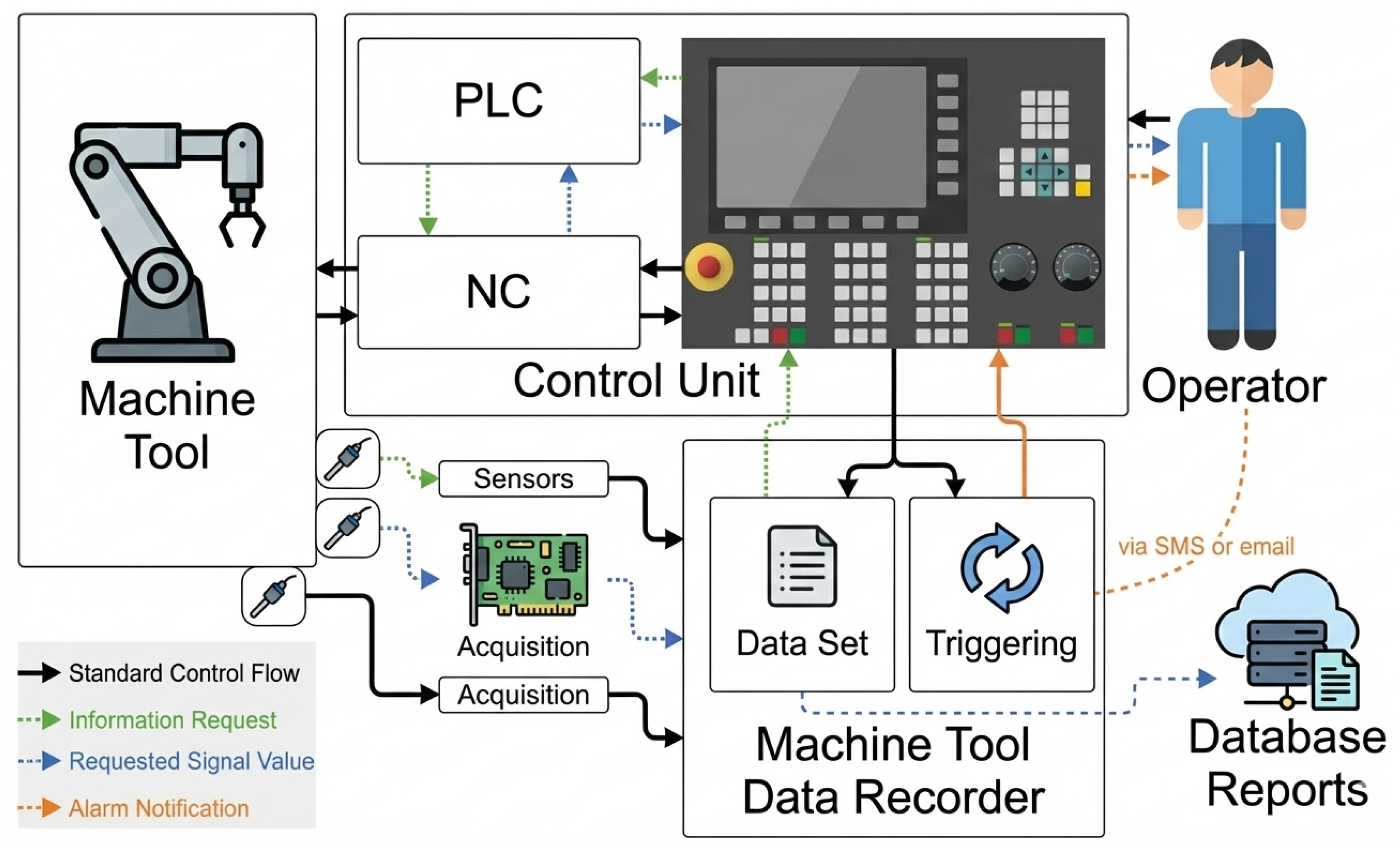
Before sensor streams can support maintenance decisions, they must be cleaned, synchronized, and reduced [6]. Noise removal, time alignment, and treatment of dropouts prepare raw signals for feature construction [7]. Multi-scale summarization then condenses the streams into overlapping windows so that rapid transients and slow wear trends are preserved together [8]. Typical descriptors include root mean square energy, spectral band energies, envelope statistics, sample entropy, and higher-order moments [9]. Cross-sensor features capture electromechanical couplings through rolling correlations, lead and lag statistics, and coherence measures that reveal which channels tend to lead or follow during anomalous events [10]. Domain-informed transforms such as targeted band-pass filtering and envelope extraction emphasize machine-specific resonances and modal behavior [11]. Together, these representations reduce data volume, stabilize distributions, and concentrate diagnostic information for downstream models [12]. Figure 1 illustrates the enhanced predictive maintenance data flow and control architecture adopted in this study.

At the modeling stage, a predictive maintenance framework must satisfy two demanding requirements: capturing long-range temporal dependencies that encode progressive wear, while producing outputs that engineers can interrogate and trust [14,15]. Sequence models for prognostics span recurrent architectures, attention-based encoders, and temporal convolutional networks [16], yet high-capacity designs often require extensive labeled data, long training times, and substantial compute, complicating routine retraining and on-site upkeep [17]. Practical adoption also demands interpretable diagnostics such as ranked feature importances, temporal saliency maps, and calibrated uncertainty so that maintenance decisions rest on transparent evidence [18]. Deployment evaluation should go beyond aggregate accuracy to include parameter counts, footprint, latency, peak memory, and end-to-end profiling [19]. Robustness under distribution shifts and sensor faults, together with reproducible modular frameworks that log preprocessing, architecture, and data splits, enables safer staged rollouts [20].

Within this context, the present study pursues three tightly linked research objectives. The first objective is to design a step-by-step predictive maintenance framework that covers data cleaning, feature extraction, temporal modeling, and visual analytics [21]. The second objective is to train a lightweight model that can both classify tool health states and estimate remaining useful life with accuracy compatible with shop-floor decision making [22]. The third objective is to evaluate the resulting framework under realistic factory constraints, with particular attention to real-time responsiveness, computational efficiency, and interpretability for engineers and operators [23]. This study integrates these elements into a single reproducible framework that is engineered for shop-floor deployment rather than offline analysis. It presents an end-to-end framework that couples multi-scale windowed feature construction with a lightweight multi-task temporal model that jointly outputs discrete health-state predictions and continuous remaining useful life estimates within one inference pass [24]. It also reports a deployment-oriented evaluation protocol covering predictive accuracy together with latency, memory footprint, robustness under realistic distribution shifts and sensor fault scenarios, and interpretable visual explanations to support engineer validation and staged rollout.

The remainder of this paper is organized as follows: Section 2 reviews related work, Section 3 details the methodology, Section 4 presents results, Section 5 discusses and compares findings and Section 6 concludes the study.

2. Literature Review

This section reviews recent research on predictive maintenance for machine tools, focusing on sensor-based condition monitoring, feature engineering and temporal learning models for health assessment and prognostics. It contrasts traditional threshold and physics-guided frameworks with data-driven and deep sequence methods. It also identifies recurring limitations in robustness, interpretability and deployment readiness that motivate the proposed framework.

2.1. Classical Statistical and Machine Learning Approaches

Predictive maintenance research has gradually shifted from classical statistical techniques toward a data-centric discipline that integrates modeling, feature engineering, and operational constraints. Bucay-Valdiviezo et al. [25] highlighted how regression-based prognostics, principal component analysis (PCA) for anomaly detection, and autoregressive integrated moving average (ARIMA) models for trend forecasting can provide interpretable signals under tightly controlled experiments and small-scale deployments. However, they also showed that such methods often fail to generalize under real production variability, sensor noise, and pronounced class imbalance. As sensor instrumentation has proliferated and labeled run-to-failure traces have become available, Hoffmann Souza et al. [26] documented a pivot toward supervised learning pipelines in which engineered windows and domain-informed features are supplied to tree-based learners and gradient-boosting machines. These models improved detection and classification accuracy in many industrial settings while retaining some degree of explainability through feature-importance measures and rule extraction.

2.2. Deep Learning and Sequence Modeling

The emergence of deep learning introduced end-to-end temporal representation learning that reduced dependence on handcrafted features. Mienye et al. [27] reviewed how recurrent networks based on long short-term memory units and gated recurrent units became early favorites because they capture sequence dependencies in a natural way. Yet recurrent architectures remain challenging in factory environments because stepwise processing slows inference and complicates training when sequences grow long [28]. Wei and Wang [29], and other authors, therefore turned to models grounded in convolution and attention. Bednarski et al. [30] reported that temporal convolutional networks can match or surpass recurrent models on many benchmarks while offering faster execution, better parallelism, and more predictable use of computing resources.

2.3. Temporal Convolutional Networks and Hybrid Architectures

Temporal convolutional networks extend their temporal reach through causal dilated filters that enlarge the receptive field as depth increases [31]. Singh [32] showed that residual connections, separable (depthwise/pointwise) convolutions, and attention modules can improve sensitivity to intermittent intervals while controlling parameter growth. Comparative studies emphasize that large convolutional and recurrent architectures differ markedly in model size, speed, and memory footprint, giving engineers concrete trade-offs when selecting models for deployment [33]. Hybrid strategies explored by Zhang et al. [34] and Zhang et al. [35] pair compact convolutional encoders with lightweight attention heads to produce multi-scale health indicators and interval-level uncertainty estimates while keeping the overall architecture manageable for industrial integration.

2.4. Benchmark Datasets and Dataset Realism

Dataset realism and scale strongly influence which methods can be transferred from laboratory studies to production lines. The commercial modular engine simulator dataset studied by the NASA community [36] provides canonical multivariate sequences with multiple operating regimes and detailed diagnostics that are well suited to remaining useful life research in aero-engines. Bearing repositories such as the XJTU-SY collection [37] offer accelerated run-to-failure traces that stress vibration-based methods and demand robustness to nonstationary statistics. Milling datasets described by Figshare contributors [38] more closely resemble shop-floor conditions because they contain high-rate vibration, acoustic emission, spindle current, force, and torque signals recorded across many extended test runs. The size imbalance and operational heterogeneity in these collections require careful choices in segmentation, rebalancing, augmentation, and validation protocols in order to avoid overly optimistic performance estimates [39].

2.5. Explainability, Robustness and Deployment Considerations

Explainability and operational diagnostics remain decisive for real industrial adoption. Kozielski [40] demonstrated that ranked sensor importances, temporal saliency maps, and entropy-based ambiguity indicators enable engineers to validate alarms against observable machine behavior and reduce costly false positives and negatives. From a deployment standpoint, Bala et al. [41] stressed the importance of profiling model parameter counts, disk footprint, inference latency, and memory usage to ensure compatibility with industrial computing stacks and to plan for versioning and updates. The same authors also showed that robustness evaluation under distributional shift and simulated sensor faults is essential to quantify graceful degradation [42]. Taken together, these strands motivate framework designs that balance predictive accuracy, computational cost, and operator trust, and they lead naturally to pipelines that combine multi-scale segmentation, cross-sensor fusion, and residual-informed features so that performance and interpretability metrics can be reported alongside practical deployment profiles [41].

Table 1. Categorized comparison of predictive maintenance methods with emphasis on temporal modeling, explainability, robustness and deployment readiness.

Category	Data/Task	Core Method	T	X	R	D	Gap
Statistical baselines [25]	Small-scale signals	Regression, PCA, ARIMA	∆	✓	✗	✗	Noise and shift sensitive
Tree based ML [26]	Windowed features	Random forest, GBDT	∆	∆	∆	✗	Feature design needed
RNN models [27,28]	Long sequences	LSTM, GRU	✓	✗	∆	✗	Slow on long horizons
Temporal convolution [30,31]	Multivariate series	Causal dilated conv	✓	✗	∆	∆	XAI often external
Conv plus attention [32,34,35]	Multi-scale signals	Residual conv, attention	✓	∆	∆	∆	Limited stress testing
XAI focus [40]	Alarm validation	Importances, saliency	∆	✓	∆	✗	Weak profiling
Deployment focus [33,41]	Edge constraints	Footprint, latency, memory	∆	∆	∆	✓	Often conceptual
Proposed framework [30,35,41]	Multisensor windows	Lightweight TCN, attention, multi task	✓	✓	✓	✓	Single domain evaluation

Legend: T temporal modeling, X explainability, R robustness, D deployment profiling. ✓ addressed, ∆ partial, ✗ not addressed.

summarizes the main methodological trends in predictive maintenance and highlights their complementary strengths and weaknesses.

Classical statistical and tree-based frameworks deliver interpretable decisions yet struggle with complex temporal structure and rarely report detailed deployment metrics. Deep recurrent and attention-based models offer powerful sequence modeling but introduce heavy training cost, higher latency, and limited transparency for operators. Recent TCN and hybrid attention architectures move closer to practical use through improved efficiency and multi-scale representations, although they often remain tied to simulator benchmarks and do not fully characterize edge resource budgets. The framework proposed in this study addresses these gaps by combining multiscale feature extraction on a realistic milling dataset with a compact temporal convolutional encoder and a lightweight attention module. The framework delivers joint tool health classification and remaining useful life estimation and couples these predictions with attention rollouts and attribution scores that expose the contribution of individual sensors and time intervals. In addition, the framework reports parameter count, memory footprint, and inference latency under an industrial-style hardware baseline, providing an end-to-end view from raw signals to deployable predictive maintenance decisions that is largely absent from prior work summarized in Table 1.

2.6. Main Contributions of This Work

The main contributions of this study are summarized as follows:

• A unified, end-to-end predictive maintenance framework integrating multiscale feature extraction, cross-sensor fusion, and temporal modeling for realistic milling data.
• A lightweight multi-task TCN-based model that jointly performs tool health-state classification and remaining useful life (RUL) estimation in a single inference pass.
• An interpretable diagnostic pipeline using attention rollouts and attribution methods to expose sensor- and time-level contributions.
• A deployment-oriented evaluation protocol reporting not only accuracy, but also latency, memory footprint, and parameter count on industrial-style hardware.
• A comprehensive experimental validation on a realistic milling dataset covering Healthy, Worn, and Failed tool conditions.

3. Methodology

This section details the systematic framework used to design, implement and evaluate the proposed predictive maintenance model. It outlines the data preprocessing procedures, model architecture, interpretability strategies and performance evaluation metrics adopted to ensure both technical rigor and practical deployability.

3.1. Methodology Overview

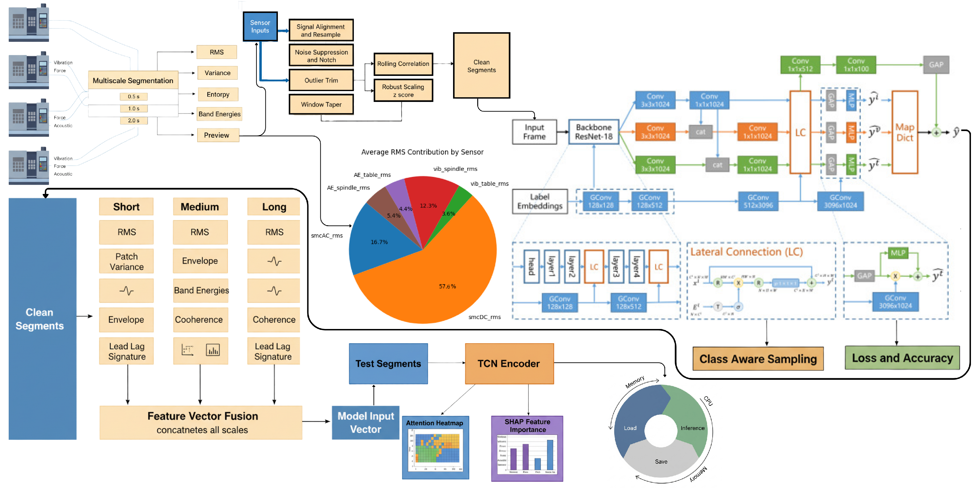
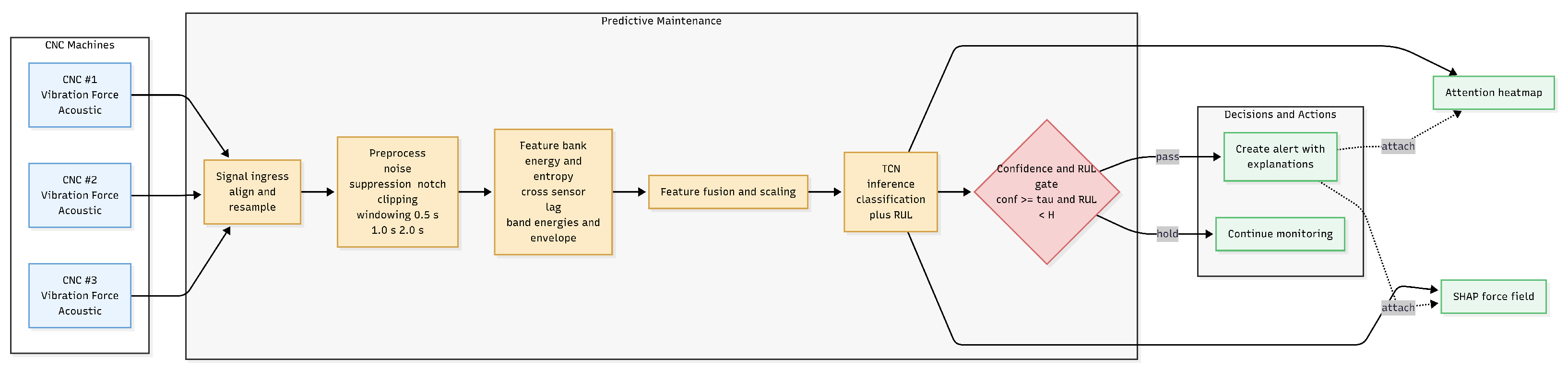
The proposed method is organized as a modular, end-to-end workflow that converts raw multi-sensor streams into actionable maintenance decisions. Rather than treating prediction as a single black-box step, the framework decomposes the process into a sequence of stages covering signal preparation, multiscale representation learning, sensor prioritization, temporal modeling, and deployment-oriented evaluation. This organization ensures that intermediate representations are explicit, reusable, and verifiable, and that the complete processing chain can be reproduced and profiled under realistic operating constraints. An overview of the full flow is shown in Figure 2 and Figure 3.

At the system level, the workflow accepts synchronized time series from multiple sensors (vibration, acoustic emission, spindle currents, and force) and produces two coupled outputs: a discrete tool health-state estimate and a continuous remaining useful life prediction. Between these endpoints, the data are transformed through preprocessing, windowing, feature construction, and a causal Temporal Convolutional Network (TCN) encoder.

Table 2. High-level structure of the proposed workflow and its intermediate artifacts.

Stage	Input	Output/Artifact
Signal preparation	Raw multi-sensor streams	Cleaned, synchronized windows
Multiscale feature construction	Windowed signals	Fixed-length feature vectors
Sensor prioritization	Training features	Selected sensor and feature subsets
Temporal modeling (TCN)	Feature sequences	Health-state probabilities and RUL estimate
Diagnostic analysis	Model internals and outputs	Feature attributions and temporal saliency maps
Evaluation and profiling	Predictions and explanations	Accuracy and deployment metrics

summarizes the main stages and their corresponding artifacts.

Beyond predictive accuracy, the framework is designed to expose how decisions are formed. Feature-level attribution is obtained using Shapley-value decomposition (Equation (12)), which expresses each prediction as a sum of contributions from the underlying features. This makes it possible to associate individual outputs with specific sensor channels and time-derived descriptors. Complementarily, attention rollout maps produced by the temporal encoder highlight which portions of the input sequence carry the greatest influence on the final decision. Together, these views provide a compact and operationally meaningful account of model behavior, allowing engineers to relate alarms and degradation trends back to observable machine signals rather than treating the model as an opaque component.

The following subsections detail each stage of this workflow, from data preparation and feature engineering to modeling, evaluation, and deployment considerations.

3.2. Dataset and Preprocessing

3.2.1. Dataset Origin, Access, and Structure

All experiments are conducted on the NASA Ames Milling dataset [43,44], a publicly available benchmark for tool condition monitoring in CNC milling. The dataset is released online by NASA and is organized as multiple milling runs recorded under controlled cutting settings. Each run provides synchronized multivariate time series from multiple sensors and an associated tool health annotation. In this study, we use vibration, acoustic emission (AE), spindle motor current AC (smcAC), spindle motor current DC (smcDC), and force. The label space contains three states: Healthy, Worn, and Failed.

Table 3. Overview of the NASA Ames milling dataset with sensor composition and average RMS statistics across multiple window scales.

Property	Description/Value	Notes
Dataset Overview
Dataset	NASA Ames Milling, public benchmark	CNC milling tool condition monitoring
Dataset structure	Multiple runs, multi-sensor time series	Each run provides synchronized channels and a tool state label
Access	Public online release by NASA	Source link and file list reported in Data Availability Statement
Sensors used in RMS summary	Vibration, AE, smcAC, smcDC	Multi-sensor subset used for RMS statistics
Additional sensor channels	Force	Present in acquisition, retained for downstream analysis
Labels	Healthy, Worn, Failed	Three tool health states
Window scales	0.5 s, 1.0 s, 2.0 s	Overlapping segmentation at three scales
Data traits	High-frequency, noisy, imbalanced	Requires cleaning, normalization and balancing
Average RMS Values per Sensor Across Window Scales
smcAC	0.388 average across windows	Current channel RMS magnitude
smcDC	1.346 average across windows	Dominant energy contributor
Vibration	0.286 average across windows	Mechanical response indicator
AE	0.126 average across windows	High-frequency acoustic bursts
Force	Included in raw acquisition	Force channel retained for downstream features

summarizes the sensor composition used in this work and reports RMS statistics computed from the windowed samples. The official dataset source link, the list of files used, and the parsing scripts that convert raw recordings into model-ready samples are reported in the Data Availability Statement to ensure full accessibility and repeatability.

The NASA Ames milling dataset consists of multiple run-to-failure milling experiments in which a cutting tool is progressively worn under controlled machining conditions. Sensors are mounted on the spindle and machine structure to record vibration, acoustic emission, spindle motor current (AC and DC), and cutting forces during operation. The tool condition evolves naturally from an initial healthy state to a progressively degraded (Worn) state and finally to a Failed state, where surface quality and cutting stability degrade beyond acceptable limits. In this dataset, the label Worn denotes an intermediate wear stage in which the tool is still operational but exhibits measurable degradation compared to the healthy baseline. The dataset contains multiple full machining runs sampled at high frequency, resulting in several million raw time samples in total. Detailed file lists, run identifiers, and acquisition parameters are provided in the public release and are referenced in the Data Availability section.

3.2.2. Sample Structure and Windowing

A supervised sample is defined as a multi-sensor segment obtained by multi-scale sliding-window segmentation at 0.5 s, 1.0 s, and 2.0 s.

This design captures short transient events as well as longer wear progression signatures. All sensor channels within a window are treated as one multichannel sample, and the corresponding sample inherits the tool health label for that run. Across the three window scales, the average RMS values indicate that smcDC exhibits the highest energy with an average of 1.346, followed by smcAC at 0.388, vibration at 0.286, and AE at 0.126, which is consistent with the dominant magnitude of the DC current channel in the acquisition.

3.2.3. Preprocessing

The preprocessing in

Table 4. Signal preprocessing pipeline steps, parameter choices and resulting outputs applied consistently before model training and evaluation.

Step	Action	Params	Out
Quality checks	Missing values and outliers	Interp, percentile clip	✓
Denoising	Noise suppression and drift removal	Low-pass, detrend	✓
Segmentation	Multi-scale windows	0.5 s, 1.0 s, 2.0 s	✓
Cross-correlation	Sensor coupling	Rolling corr, lags	✓
Feature extraction	Window-level statistics	RMS, var	✓
Scaling	Standardize features	z-score train stats	✓
Balancing	Rebalance training only	Resample	✓
Diagnostics	Visual sanity checks	Spectrogram, radar	✓

converts the raw multi-sensor time series into clean and comparable inputs for model training. First, each sensor channel is inspected for missing samples and obvious spikes, then corrected by linear interpolation for short gaps and clipped for extreme outliers using percentile-based thresholds. Second, sensor signals are denoised using a low-pass filtering step to suppress high-frequency measurement noise while preserving fault-related dynamics, and a detrending step is applied when slow drift is observed in current channels smcAC and smcDC. Third, the cleaned streams are segmented into 0.5 s, 1.0 s, and 2.0 s windows to capture both short transients and progressive wear patterns. Fourth, features are extracted from each window using statistical descriptors such as RMS and variance, and inter-sensor relationships are quantified using rolling cross-correlation with multiple lags. Fifth, feature scaling is performed by z-score standardization using the mean and standard deviation computed from the training split only, and the same parameters are applied to validation and test data to prevent data leakage. Sixth, class imbalance is handled by resampling the training set only, while validation and test distributions are kept unchanged to reflect the real operating conditions. Finally, diagnostic checks using spectrograms and radar charts are performed to confirm that filtering, scaling, and windowing preserve meaningful signatures and do not introduce preprocessing artifacts.

3.3. Feature Selection via Residual-Based Sensor Prioritization

To make the feature selection step explicit, we adopt a residual-based sensor prioritization strategy. The key idea is to compute per-sensor residual signals, summarize their residual energy over windowed segments, and convert these energies into normalized importance weights that drive sensor selection and feature group prioritization. All residual statistics and selection decisions are computed using the training split only, and the selected sensor set is then fixed for validation and testing to avoid data leakage.

For each sensor channel c, we form a residual signal by subtracting a reference signal ${\widehat{x}}_{c,t}$ from the observed sample $x_{c,t}$. The reference can be a healthy profile estimate or a baseline predictor used only to reveal deviations.

$$r_{c,t}=x_{c,t}-{\widehat{x}}_{c,t}$$

(1)

In Equation  (1), $r_{c,t}$ denotes the residual for channel c at time t, $x_{c,t}$ is the raw measurement and ${\widehat{x}}_{c,t}$ is the corresponding reference value.

Residual overlays are summarized by a window-level residual energy score per channel. For window index n with sample set ${\mathcal{W}}_n$, the residual energy is defined as

$$E_{c,n}={\displaystyle \frac{1}{\left|{\mathcal{W}}_n\right|}}\sum _{t\in {\mathcal{W}}_n}{r}_{c,t}^2$$

(2)

In Equation (2), $E_{c,n}$ is the residual energy of channel c in window n, and $\left|{\mathcal{W}}_n\right|$ is the number of samples in that window.

We aggregate window energies into a single training split score ${\overline{E}}_c$ and normalize it into an importance weight ${\alpha }_c$. A binary selection variable $s_c$ is then obtained using a threshold $\theta$.

$${\alpha }_c={\displaystyle \frac{{\overline{E}}_c}{{\sum }_{j\in \mathcal{C}}{\overline{E}}_j}}\hspace{1em}\hspace{1em}{s}_c=\mathbb{I}\left[{\alpha }_c\ge \theta \right]$$

(3)

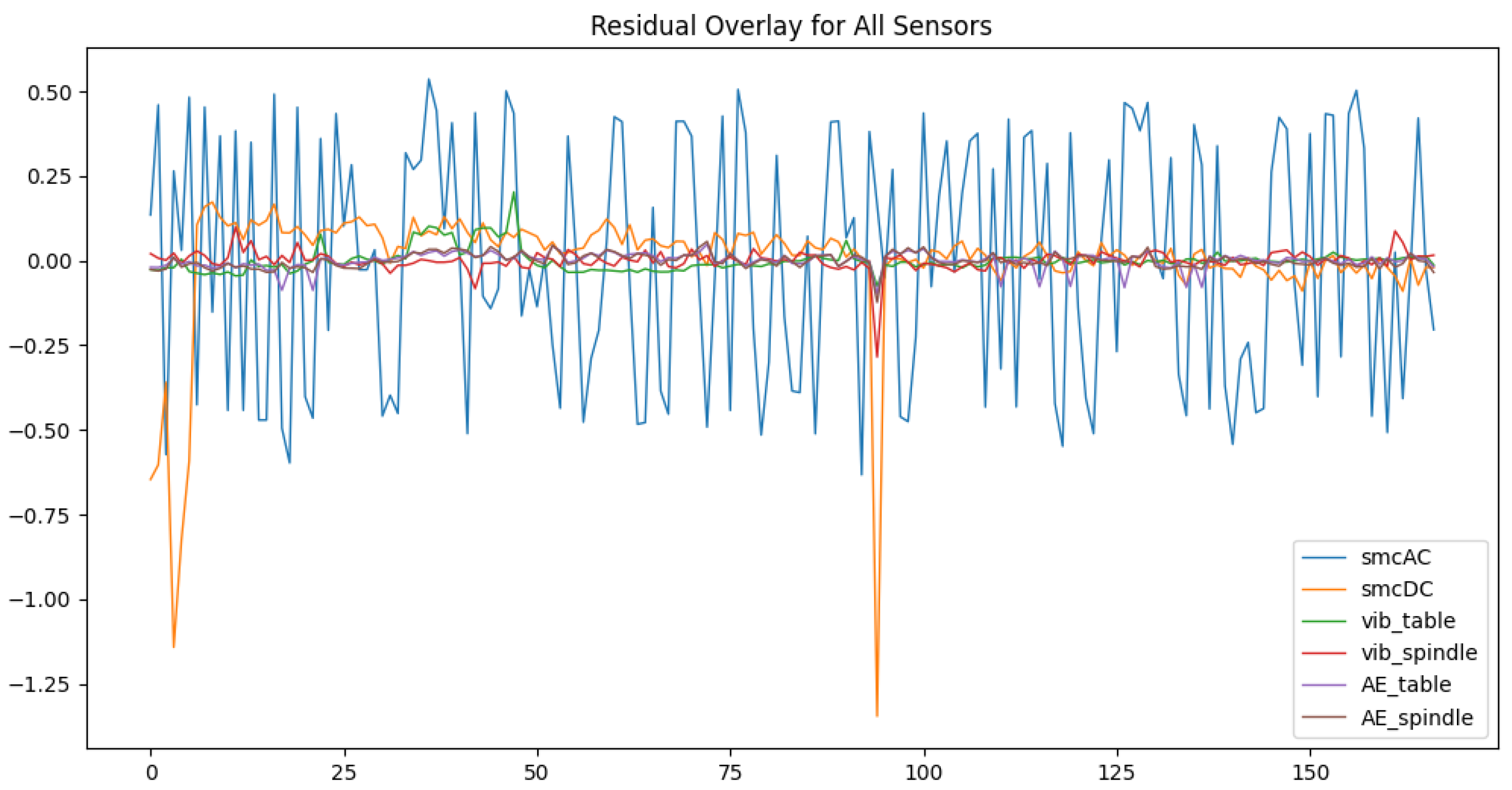
In Equation (3), $\mathcal{C}$ denotes the set of sensor channels, ${\overline{E}}_c$ is the mean residual energy across training windows for channel c, ${\alpha }_c$ is the normalized importance weight, $\theta$ is the selection threshold and $s_c$ indicates whether the channel is retained for downstream feature construction.

Table 5. Residual-based sensor prioritization for feature selection using training split residual energy.

Sensor Channel	${\overline{\mathit{E}}}_{\mathit{c}}$ Mean Residual Energy	${\mathit{\alpha }}_{\mathit{c}}$ Normalized Importance	Selected ${\mathit{s}}_{\mathit{c}}$
Vibration	$0.02\pm 0.03$	$0.006$	no
Acoustic emission (AE)	$0.01\pm 0.01$	$0.003$	no
Spindle motor current AC (smcAC)	$2.6\pm 0.6$	$0.781$	yes
Spindle motor current DC (smcDC)	$0.7\pm 1.3$	$0.210$	yes

reports the residual energy statistics and the resulting selection decision per sensor. The selected channels define the final feature set by retaining all engineered features derived from channels with $s_c=1$, while dropping features from channels with $s_c=0$. This makes the feature selection stage transparent and directly tied to the residual overlay evidence.

3.4. Mathematical Modeling of Framework

Multiscale segmentation compresses raw high-rate streams into scale-specific summaries that preserve both short transients and long degradation trends while producing fixed-size inputs for the sequence model. See Equation (4) for the formal aggregation of per-scale summaries into a per-segment feature vector.

$${\mathbf{F}}_n={\left[ {\mathcal{G}}_s\left(X_{t_n-{\tau }_s:t_n}\right) \right]}_{s\in \mathcal{S}}$$

(4)

In Equation (4), the symbol ${\mathbf{F}}_n$ denotes the concatenated feature vector for segment index n, ${\mathcal{G}}_s$ denotes the summary mapping at scale index s, $X_{a:b}$ denotes the multivariate sensor matrix spanning sample indices a through b, ${\tau }_s$ denotes the time length of scale s and $\mathcal{S}$ denotes the finite set of scales used in the framework.

Windowed energy estimates reduce sensitivity to window edges while emphasizing per-channel power that is diagnostic of wear. See Equation (5) for the tapered root mean square used to form energy descriptors.

$${\mathrm{RMS}}_c\left(t;w,h\right)=\sqrt{{\displaystyle \frac{{\sum }_{i=0}^{w-1}h\left(i\right) x_{c,t-i}^2}{{\sum }_{i=0}^{w-1}h\left(i\right)}}}$$

(5)

In Equation (5), the index c identifies the sensor channel, t denotes the current sample time, w denotes the window length in samples, $h\left(i\right)\ge 0$ denotes the taper weight at lag i and $x_{c,t}$ denotes the raw sample for channel c at time t.

Local normalized cross correlation reveals lead and lag relationships between sensor pairs that can indicate causal precedence of electrical anomalies before mechanical response. See Equation (6) for the local Pearson style correlation computed over a sliding window.

$$\begin{array}{cc}\hfill {\rho }_{c_1,c_2}\left(t,\ell ;w\right) & ={\displaystyle \frac{{\sum }_{i=0}^{w-1}\left(x_{c_1,t-i}-{\mu }_{c_1,t}\right)\left(x_{c_2,t-i-\ell }-{\mu }_{c_2,t-\ell }\right)}{\sqrt{{\sum }_{i=0}^{w-1}{\left(x_{c_1,t-i}-{\mu }_{c_1,t}\right)}^2}}}\hfill \\ \hfill & \times {\displaystyle \frac{1}{\sqrt{{\sum }_{i=0}^{w-1}{\left(x_{c_2,t-i-\ell }-{\mu }_{c_2,t-\ell }\right)}^2}}}\hfill \end{array}$$

(6)

In Equation (6), the indices $c_1$ and $c_2$ denote the two sensor channels, ℓ denotes the integer lag, w denotes the window length, $x_{c,t}$ denotes raw samples and ${\mu }_{c,t}$ denotes the local mean of channel c computed over the corresponding window used in the numerator and denominators.

Aggregating correlation magnitudes across a small lag range produces compact lead lag signatures that encode the timing and strength of coupling between channels. See Equation (7) for the lag aggregated absolute correlation signature.

$${\mathsf{\Lambda }}_{c_1,c_2}\left(t;w,L_{max}\right)=\sum _{\ell =-L_{max}}^{L_{max}}|{\rho }_{c_1,c_2}\left(t,\ell ;w\right)|$$

(7)

In Equation (7), ${\mathsf{\Lambda }}_{c_1,c_2}$ denotes the aggregated absolute local correlation between channels $c_1$ and $c_2$, $L_{max}$ is the maximum lag considered and $\rho$ is the local correlation defined in Equation (6).

Spectral band energies isolate energy in frequency bands of interest so that resonance growth or broadband noise increases are captured as separate features. See Equation (8) for per-band energy computed from a short-time spectral estimate.

$$E_{c,b}\left(t;w\right)=\sum _{f\in {\mathcal{B}}_b}{S}_c\left(t;f,w\right)$$

(8)

In Equation (8), $E_{c,b}$ denotes the energy for channel c in spectral band b at time t, ${\mathcal{B}}_b$ denotes the set of frequency bins comprising band b and $S_c(t;f,w)$ denotes the short time spectral energy for channel c at frequency bin f computed over window length w.

Patch variance after detrending quantifies localized variability while discounting slow trends that are not diagnostic of abrupt degradation. See Equation (9) for the bias-corrected patch variance.

$${\mathrm{PatchVar}}_{c,j}={\displaystyle \frac{1}{T_j-1}}\sum _{t\in {\mathcal{P}}_j}{\left(x_{c,t}-{\tilde{x}}_{c,{\mathcal{P}}_j}\right)}^2$$

(9)

In Equation (9), the index j denotes the patch identifier, ${\mathcal{P}}_j$ denotes the set of time indices in patch j, $T_j$ denotes the patch length, $x_{c,t}$ denotes raw samples and ${\tilde{x}}_{c,{\mathcal{P}}_j}$ denotes the detrended patch mean obtained by removing a local trend from the patch.

Per-channel normalization stabilizes feature scales and reduces covariate shift across segments, which improves optimization and generalization. See Equation (10) for the z-score normalization used in the framework.

$$z_{c,t}={\displaystyle \frac{x_{c,t}-{\mu }_c}{{\sigma }_c+\epsilon }}$$

(10)

In Equation (10), $z_{c,t}$ denotes the normalized value for channel c at time t, ${\mu }_c$ denotes the channel mean estimate, ${\sigma }_c$ denotes the channel standard deviation estimate and $\epsilon$ denotes a small positive constant added for numerical stability.

Causal dilated convolution implements the sequence operation in the encoder so that long-range dependencies are learned while preserving the time causality required for online inference. See Equation (11) for a single-layer dilated convolutional update.

$$y_t=\sum _{k=0}^{K-1}{w}_k x_{t-d k}$$

(11)

In Equation (11), $y_t$ denotes the layer output at time t, K denotes the convolution kernel width, $w_k$ denotes the learnable kernel weight at position k, d denotes the dilation factor and $x_{t-d k}$ denotes the input at the dilated offset.

Feature attributions provide an expectation-based decomposition of model outputs so that ranked sensor importances and local explanations can be produced for operator inspection. See Equation (12) for the Shapley value decomposition applied to model outputs.

$${\varphi }_i\left(x\right)=\sum _{S\subseteq F\setminus \left\{i\right\}}{w}_{S,F} \left[f_x\left(S\cup \left\{i\right\}\right)-f_x\left(S\right)\right]$$

(12)

In Equation (12), ${\varphi }_i\left(x\right)$ denotes the Shapley value for feature index i at input x, F denotes the full feature set, S denotes a subset of features not containing i, $w_{S,F}$ denotes the combinatorial Shapley weight for subset S relative to F and $f_x\left(S\right)$ denotes the expected model output when only features in subset S are present.

All feature mappings ${\mathcal{G}}_s$ pool and concatenate the quantities defined above to form aligned fixed-size vectors so the encoder receives consistent multiscale inputs. The equations presented together specify the core feature engineering, temporal operations and interpretability computations of the predictive maintenance framework.

3.5. Framework Architecture and Modular Flow Design

Algorithm 1 defines a modular predictive maintenance workflow that transforms raw multivariate sensor streams into deployable predictions with explanations and profiling.

Algorithm 1 PdM Framework

Require: Raw multivariate streams $\mathcal{X}$, labels $\mathcal{Y}$, optional RUL $\mathcal{R}$, scales $\mathcal{S}$ Ensure: Trained TCN $f_{\widehat{\varphi }}$, explanations $\left\{\varphi \right\}$, profiling  1. Features: multiscale windows; RMS, variance, spectral bands; lag correlations  2. Prepare: per-channel standardization; imbalance handling  3. Train: TCN encoder with heads for classification and RUL  4. Explain + evaluate: class metrics; attributions and saliency  5. Profile: parameters, size, latency, peak memory, end-to-end runtime  6. return $f_{\widehat{\varphi }},\left\{\varphi \right\},\mathrm{metrics},\mathrm{profile}$

Multiscale segmentation produces fixed-length representations (Equation (4)) using energy and variability (Equation (5)), lag structure (Equations (6) and (7)) and band energies (Equation (8)), followed by normalization (Equation (10)). The temporal convolutional encoder (Equation (11)) predicts health state and remaining useful life, while Shapley decomposition (Equation (12)) attributes sensor contributions.

Figure 2 visualizes the full modular flow, aligning preprocessing, feature extraction, training, explainability, evaluation and profiling with the mathematical definitions above.

The diagram highlights how multiscale features and lag-based coupling descriptors are passed forward into the learning and diagnostic blocks in a reproducible sequence. Figure 3 provides a condensed end-to-end summary from acquisition to decisions, emphasizing the two model outputs and the operator-facing explanation artifacts.

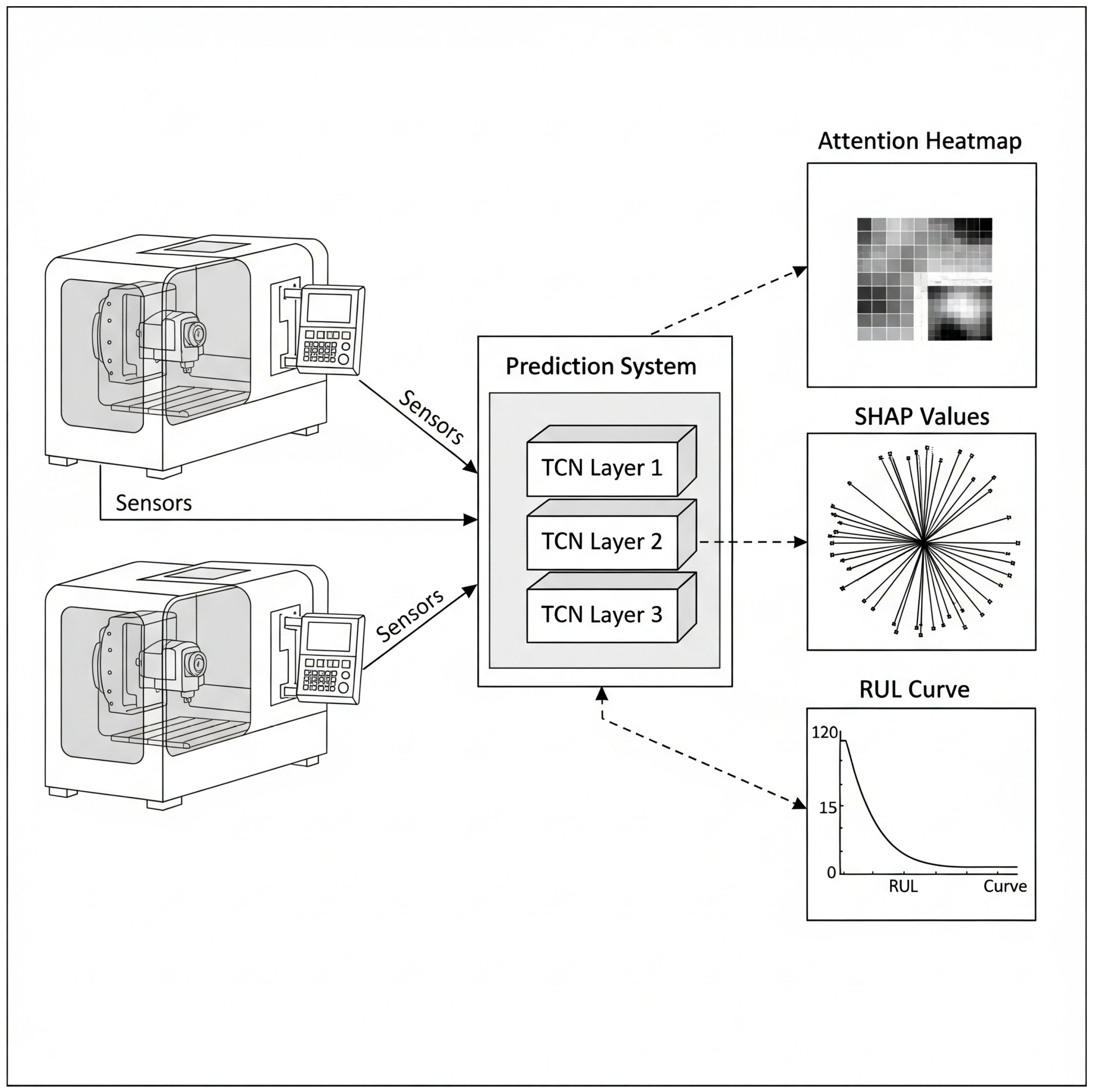
This view is used as a compact reference for the inference path and the points where explanations are generated for validation. Finally, Figure 4 situates the framework in its deployment context, illustrating a conceptual multi-machine sensing scenario with centralized inference and diagnostic feedback to support maintenance planning. In this study, however, experimental validation is conducted using data from a single CNC machine, and multi-machine deployment is left as future work.

In operation, the framework streams features to the TCN in real-time and logs predictions, explanations, and profiling statistics for monitoring and rollout.

3.6. Model Hyperparameters, Hardware and Software Configuration

3.6.1. Hyperparameter Search Strategy

Model selection was performed using a structured grid search to balance predictive performance, training stability, and deployment efficiency. The search space covered both architectural and optimization-related parameters, including network depth and width, kernel size, dilation scheme, residual connections, regularization strength, learning rate, and batch size. The full set of hyperparameters and candidate values explored during tuning is reported in

Table 6. Hyperparameter search space explored during grid search for the TCN backbone and training configuration.

Hyperparameter	Values
Number of TCN layers	{3, 4, 5}
Hidden units per layer	{32, 64, 128}
Kernel size	{2, 3, 5}
Dilation scheme	{Linear, Exponential}
Residual connections	{Enabled, Disabled}
Dropout rate	{0.1, 0.2, 0.3}
Learning rate	1 × 10−4, 5 × 10−4, 1 × 10−3
Batch size	{32, 64, 128}
Loss weight (classification vs. RUL) $\lambda$	{0.3, 0.5, 0.7}

.

3.6.2. Joint Model Selection for Diagnostics and Prognostics

Because the proposed network jointly performs health-state classification (diagnostics) and remaining useful life (RUL) regression (prognostics), hyperparameter tuning was treated as a multi-objective selection problem. For each candidate configuration, we evaluated (i) macro-F1 score on the validation set for classification and (ii) mean absolute error (MAE) for RUL prediction, together with basic efficiency indicators such as inference latency. Rather than optimizing a single task in isolation, the final model was chosen as a Pareto-optimal trade-off that provides stable and competitive performance on both tasks while keeping computational cost moderate. This ensures that a single shared backbone is suitable for unified deployment in industrial settings.

3.6.3. Final Selected Configuration

The resulting configuration selected from the grid search is summarized in

Table 7. Temporal Convolutional Network architecture, optimization and training hyperparameters employed consistently across all experimental evaluations.

Setting	Value
Search strategy	Grid search, accuracy-stability-efficiency trade-off
Model type	Temporal Convolutional Network
Convolutional layers	4
Hidden units per layer	64
Kernel size	3
Dilation and residuals	Enabled
Dropout	0.2
Optimizer	Adam
Learning rate	$1\times {10}^{-3}$
Batch size	64
Tasks	Health-state classification and RUL regression
Loss	Cross-entropy plus mean squared error

. This configuration is used consistently across all experiments, including robustness evaluations and deployment profiling.

3.6.4. Hardware and Software Baseline

All training, validation, and profiling experiments were conducted using the fixed hardware and software environment reported in

Table 8. Minimum hardware and software configuration used for model training, inference profiling and experimental reproducibility.

Component	Specification
CPU	Intel Core i7 class
Memory	16 GB RAM
Storage	50 GB free disk
GPU	Optional for faster training
OS	Ubuntu 20.04 or Windows 10
Python	3.10
Core libraries	NumPy (v1.26.4), pandas (v2.1.4), scikit-learn (v1.4.0), PyTorch (v2.1.0)
Recorded during runs	Wall-clock time, memory use, inference throughput

. Reporting results under a fixed baseline ensures that latency, memory usage, and throughput measurements are directly comparable across model variants and experimental conditions.

3.7. Evaluation Protocol

This subsection clarifies the evaluation protocol used to obtain all predictive, interpretability, and deployment results. The protocol is summarized in

Table 9. Evaluation protocol used for training, model selection, testing, and deployment profiling.

Protocol Item	Specification Used in This Work
Split unit	Run level split so all segments from one run stay in one split
Split ratios	Training 70%, validation 15%, test 15% using stratified assignment over labels
Segmentation timing	Windowing performed after run assignment to enforce leakage free splits
Preprocessing fit	Fitted on training split only then applied to validation and test
Scaling	Z-score standardization using training split mean and standard deviation only
Feature selection	Residual-based sensor prioritization computed on training split only and then fixed
Model selection	Grid search using validation split under an accuracy stability efficiency trade-off
Final training	Train on training split and select by validation performance using the fixed TCN setup in Table 7
Final test report	Single evaluation on the held out test split after model selection is complete
Classification metrics	Accuracy, precision, recall, macro F1, confusion matrix
RUL metrics	Mean absolute error, root mean squared error
Profiling metrics	Parameter count, model size, peak memory, end-to-end runtime, inference throughput
Profiling environment	Hardware and software baseline as reported in Table 8

and is designed to prevent data leakage while reporting accuracy and deployment readiness in a reproducible way.

3.7.1. Split Unit and Leakage Prevention

The unit of splitting is a machining run. All windowed segments extracted from the same run are assigned to a single split so that overlapping windows from one physical run cannot appear in both training and testing. Preprocessing steps that learn statistics from data are fitted on the training split only, then applied unchanged to validation and test, including z-score scaling and the residual-based sensor prioritization used for feature selection.

3.7.2. Model Selection and Training

Model selection follows a grid search strategy and the final Temporal Convolutional Network (TCN) training setup uses the fixed configuration reported in Table 5 of the manuscript. The validation split is used to select the best configuration under an accuracy, stability, and efficiency trade-off, then the selected configuration is evaluated once on the held-out test split and reported as the final performance.

3.7.3. Metrics and Reporting

For health-state classification, we report accuracy together with per-class precision, recall, and macro F1 to account for imbalance. For remaining useful life prediction, we report mean absolute error and root mean squared error. For deployment readiness, we report parameter count, model size, peak memory, end-to-end runtime, and inference throughput using the hardware and software baseline in Table 8 of the manuscript.

The predictive maintenance framework in Algorithm 1 provides an integrated framework that converts raw industrial sensor streams into actionable maintenance outputs using the formulations in Equations (4)–(12). Multiscale segmentation compresses high-frequency signals into fixed-length windows that retain transient events and gradual degradation. Features combine tapered energy from Equation (5), lead-lag dependencies from Equation (7) and spectral band energies from Equation (8) to fuse electrical, mechanical and acoustic cues. A causal temporal convolutional encoder in Equation (11) supports stable, real-time inference. Interpretability is built in through Shapley decomposition in Equation (12), producing sensor-level contributions rather than opaque alarms, while profiling quantifies latency and resource use for deployment. Figure 2 and Figure 3 summarize the resulting reproducible, efficient architecture.

4. Results

This section provides an overview of the dataset, the results of data cleaning, summaries of the extracted features and details about how the models were trained.

4.1. Dataset Characterization and Multiscale Feature Stability Analysis

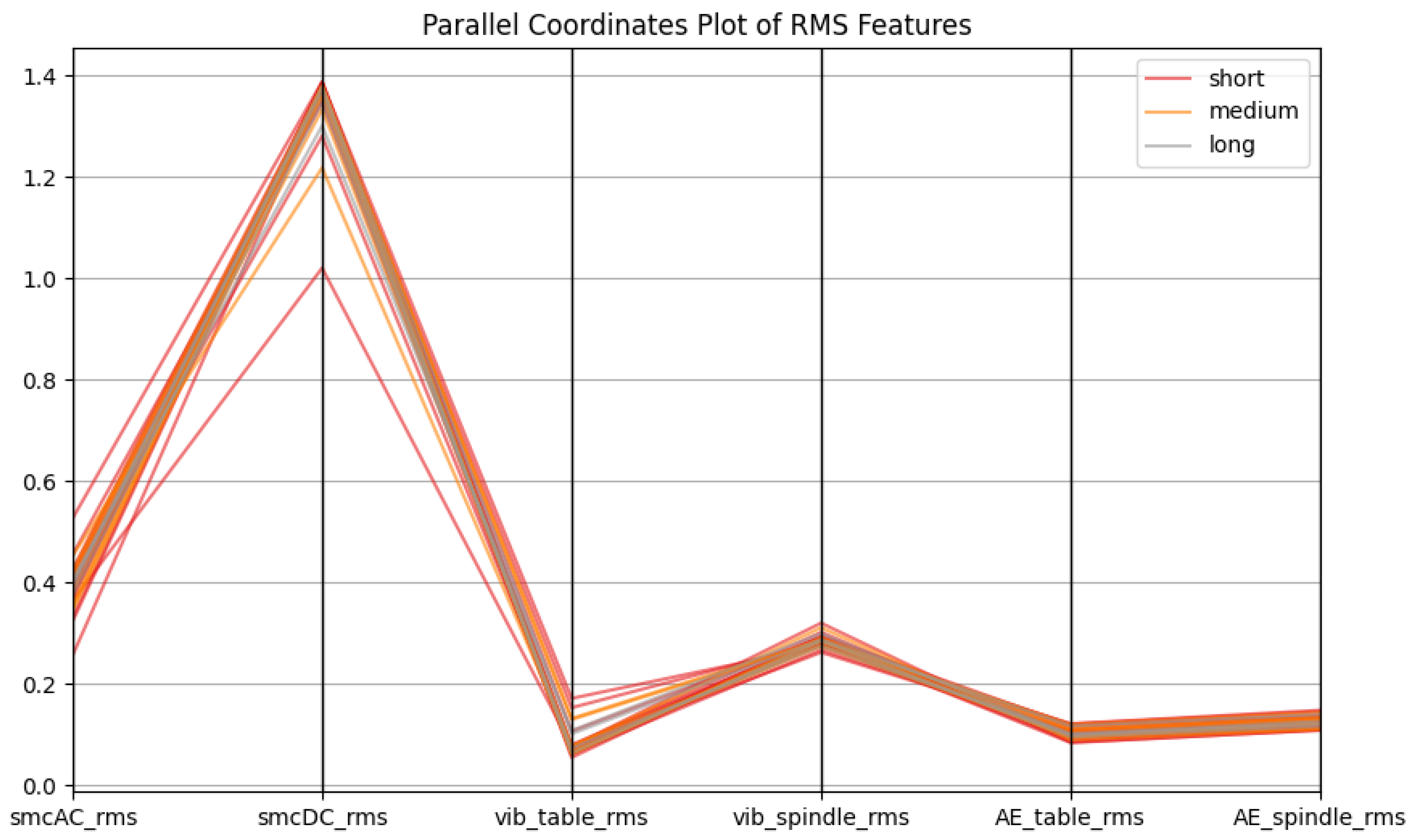
This subsection summarizes the dataset and initial stability analysis of sensor features. Multivariate streams from CNC machines, including vibration, force, acoustic emission and spindle current, were recorded under Healthy, Worn and Failed conditions, then segmented into overlapping 0.5 s, 1.0 s and 2.0 s windows to capture fast transients and gradual wear. The window-length study shows shorter windows preserve rapid variability while longer windows smooth noise and emphasize long-term trends. Cross-sensor RMS comparisons in Figure 5 indicate consistent patterns across scales, with smcDC and smcAC dominant and vibration and acoustic channels showing smaller stable responses, supporting multiscale fusion. In the following spectral and time-domain analyses, the frequency range is limited to 0–500 Hz because this band covers the dominant mechanical and electromechanical components of the milling process in the NASA Ames setup, including spindle rotation harmonics and structural vibration modes, while higher frequencies are largely dominated by sensor noise and do not contribute significantly to wear discrimination.

Table 10. Window-scale RMS statistics with variance and normalized energy contribution for current, vibration and acoustic channels. Results highlight stable cross-scale dominance of smcDC and smcAC, with vib_spn providing consistent secondary mechanical information and supporting multi-scale feature fusion for degradation monitoring.

Scale	Sensor	Mean RMS	Variance	Contr. %
0.5 s	smcAC	0.50	0.25	18.2
0.5 s	smcDC	1.38	0.78	57.7
0.5 s	vib_tbl	0.16	0.04	3.6
0.5 s	vib_spn	0.29	0.09	12.1
0.5 s	AE_tbl	0.09	0.03	4.4
0.5 s	AE_spn	0.11	0.03	4.0
1.0 s	smcAC	0.55	0.27	20.4
1.0 s	smcDC	1.36	0.75	54.9
1.0 s	vib_tbl	0.15	0.03	3.1
1.0 s	vib_spn	0.29	0.08	12.3
1.0 s	AE_tbl	0.09	0.03	4.6
1.0 s	AE_spn	0.11	0.02	4.7
2.0 s	smcAC	0.45	0.21	16.7
2.0 s	smcDC	1.34	0.74	52.3
2.0 s	vib_tbl	0.14	0.03	3.3
2.0 s	vib_spn	0.28	0.07	12.1
2.0 s	AE_tbl	0.09	0.03	4.5
2.0 s	AE_spn	0.10	0.02	4.1
All	Avg all sensors	0.41	0.18	100.0
All	Dominant sensor smcDC	1.36	0.76	55.0
All	Next sensor smcAC	0.50	0.24	18.0
All	Next sensor vib_spn	0.29	0.08	12.0
All	KDE peak vib_spn	0.29, 0.30, 0.31	0.08	12.0

reports mean RMS, variance and normalized energy contribution across window sizes. smcDC consistently dominates the energy budget at about 55%, followed by smcAC at roughly 18–20%, while vibration and acoustic channels contribute smaller but stable shares that capture complementary mechanical and acoustic behavior. The dataset contains vibration, force and acoustic emission streams from CNC machines under Healthy, Worn and Failed conditions, segmented into 0.5 s, 1.0 s and 2.0 s windows to represent both transients and gradual wear. Parallel-coordinate patterns remain coherent across scales, indicating stable cross-sensor structure. Short windows increase sample count and variability, requiring careful balancing so training is not biased toward short-term dynamics.

Taken together, the multiscale stability patterns in Figure 5 and the energy distributions summarized in Table 10 establish two key design choices for the subsequent stages of the pipeline. First, they justify the use of multiscale windowing and energy-based descriptors as a stable representation across operating conditions. Second, they motivate a more detailed investigation of cross-sensor interactions rather than treating channels independently. Accordingly, the next subsection builds on these findings by formalizing the preprocessing steps and by analyzing cross-sensor correlations, which are then explicitly encoded into the feature construction stage via lag-aggregated correlation descriptors.

4.2. Preprocessing, Cross-Sensor Correlation Analysis and Feature Construction

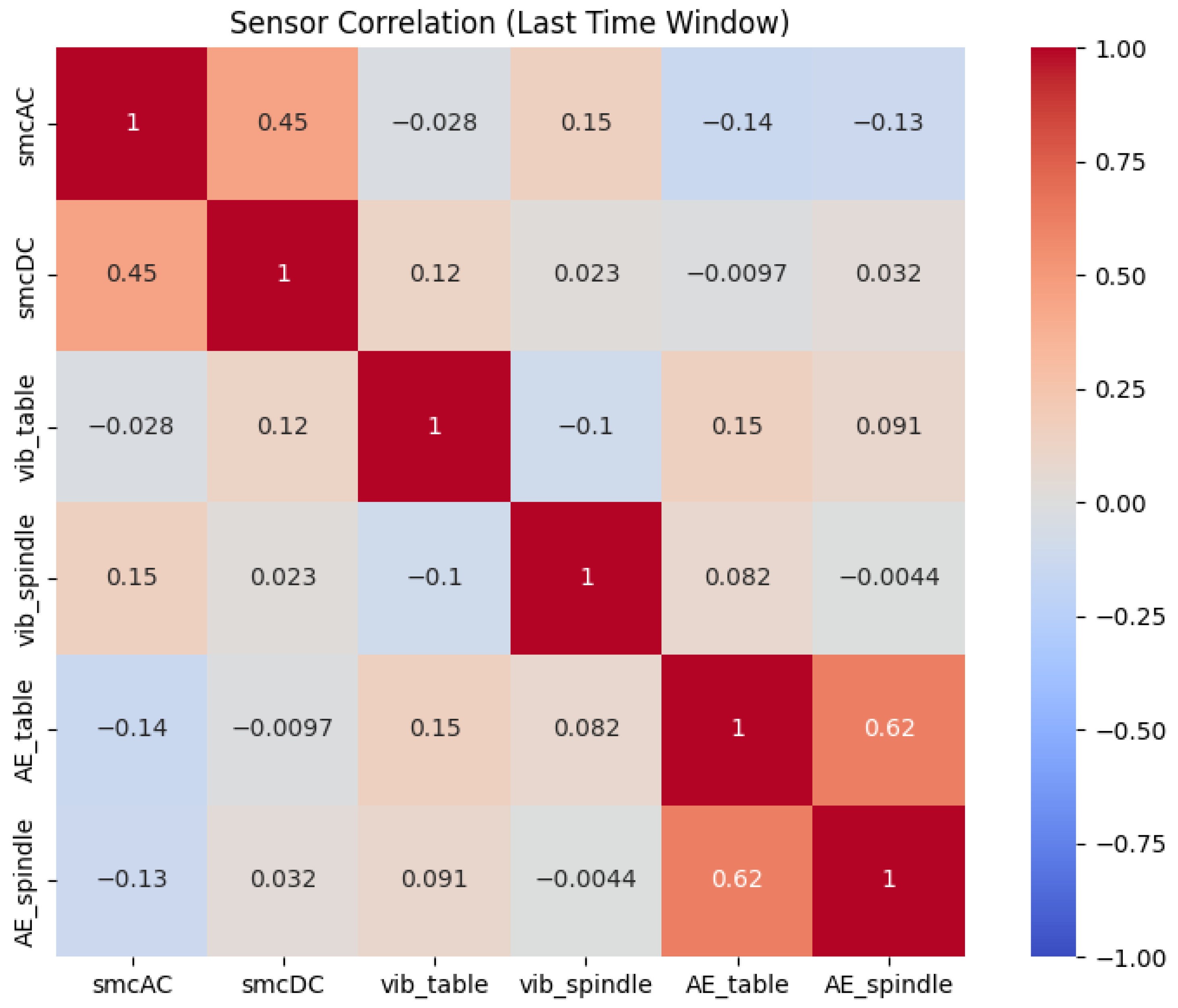
The preprocessing stage converts raw sensor streams into synchronized, denoised features for modeling. Channels are time-aligned and resampled to a common clock, then segmented into overlapping 0.5 s, 1.0 s and 2.0 s windows to capture transients and gradual wear. Each segment is tapered and bandlimited to preserve the dominant mechanical band below 500 Hz, with cleaning via median absolute deviation trimming, notch filtering at mains frequencies and calibration-based clipping. Robust scaling uses the median and interquartile range before feature extraction. Figure 6 shows the terminal-phase correlation heatmap computed using Equation (6) on z-score normalized data, revealing strong smcAC-smcDC coupling, moderate vibration-acoustic links and low off-diagonal correlations that motivate the lead-lag aggregation in Equation (7).

Before presenting the merged summary table, we describe its intent.

Table 11. Correlation, lag and spectral relationships among key sensor pairs, revealing cross-domain coupling and diagnostic timing characteristics.

Sensor Pair	Corr.	Lag	Band Hz	Domain	Key Observation
AE spindle—AE table	0.77	0	0–500	Acoustic	Strong coupling at spindle table interface
Vibration spindle—AE spindle	0.80	+100	0–500	Mech-Acous	Mechanical energy transfer to acoustic channel
smcDC—Vibration spindle	0.24	+35	0–500	Elec-Mech	Delayed electrical to mechanical response cue
smcAC—smcDC	0.45	0	Broadband	Electrical	Stable intra current coupling
Vibration spindle - Vibration table	0.07	0	Broadband	Mechanical	Low coherence provides complementary motion info
AE table—smcDC	0.21	0	Broadband	Cross modal	Weak acoustic electrical interaction
Mean correlation	0.26 with standard deviation 0.21

consolidates correlation magnitude, lag at peak cross-correlation and dominant spectral-band findings for the most informative sensor pairs, enabling practitioners to identify which channels and frequency ranges should be emphasized during feature engineering. Feature construction aggregates time- and frequency-domain descriptors into fixed-length per-segment vectors. Time-domain features include tapered RMS, patch variance, envelope statistics and rolling correlation aggregates. Frequency-domain features include band energies, spectral centroid and coherence peaks within 0 to 500 Hz. The lag at maximum correlation and the aggregated absolute correlation across the lag window are appended as lead-lag descriptors. Class and scale imbalance are reduced using stratified resampling and class-aware batching. Preprocessing artifacts, including scaling parameters, feature schema and index mappings, are versioned for reproducibility and ablations. Figure 6 supports these choices.

These correlation statistics are not reported merely for descriptive purposes. The identified strong couplings are directly used during feature construction, where lag-aggregated cross-correlation magnitudes (Equation (7)) are included as input features to the TCN model, allowing the network to exploit electromechanical lead–lag relationships during health-state and RUL prediction. While the correlation analysis in Figure 6 and the summary statistics in Table 11 determine which cross-sensor interactions should be encoded as lead–lag features, they do not by themselves indicate which individual sensor channels carry the strongest degradation signal over time. To address this complementary question, the next stage analyzes residual energy patterns across channels in order to prioritize sensors and feature groups according to their deviation from nominal behavior, thereby refining the multiscale representation before it is passed to the temporal model.

4.3. Multiscale Feature Extraction and Residual-Based Sensor Prioritization

This stage extracts compact, interpretable features that highlight deviations from nominal behavior and early wear. Per-segment energy, variance, envelope statistics, band energies and rolling correlation features are computed at short, medium and long scales and concatenated into the model input. Figure 7 overlays channel residuals to show which sensors deviate earliest and most strongly, supporting feature selection.

Prior to the compact summary table, we note its purpose. The table condenses the residual energy statistics used to prioritize sensors and to weight feature groups during training. It reports central tendency, spread and a brief diagnostic note per sensor so readers can interpret which modalities drive predictive signal energy. See

Table 12. Residual energy distribution across sensor channels, highlighting dominant electrical contributions and supporting mechanical and acoustic responses.

Sensor	Key Metrics	Role	Observation
smcAC	Mean 2.6 ± 0.6, Max 3.6	Primary driver	High residual energy with oscillatory electrical patterns
smcDC	Mean 0.7 ± 1.3, Max 3.5	Early indicator	Transient spikes linked to load variation
vib_spindle	Mean 0.02 ± 0.03, Max 0.09	Mechanical response	Low-amplitude residuals aligned with current bursts
vib_table	Range 0.02–0.10	Structural baseline	Stable response with limited variance
AE_table	Mean 0.01 ± 0.01	Validation cue	Minimal acoustic deviation, supports confirmation
AE_spindle	Mean 0.01 ± 0.01	Supporting signal	Low residuals correlated with AE table
Aggregate	-	Current dominated	Mean residual about 0.66 driven mainly by smcAC and smcDC

for the condensed residual energy summary.

Feature extraction builds fixed-length multiscale descriptors from time, spectral, cross-sensor lead-lag and residual features. Residual overlays show current channels deviate earliest, while vibration and acoustic add complementary cues, enabling stable, interpretable TCN inputs. Together, Figure 7 and Table 12 establish which sensor modalities dominate the degradation signal and how multiscale features should be weighted and composed before learning. The resulting representation is a fixed-length, multiscale feature vector that combines time-domain, spectral, lead–lag and residual-based descriptors, with emphasis placed on the most informative current channels while preserving complementary mechanical and acoustic cues. This consolidated feature set forms the direct input to the Temporal Convolutional Network, whose training dynamics and predictive performance are analyzed in the following subsection.

4.4. Model Training, Convergence Analysis and Performance Evaluation

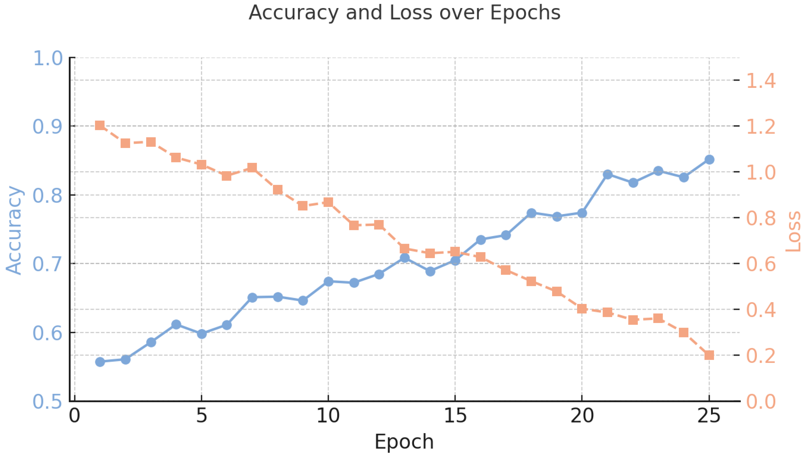
This subsection summarizes training, monitoring and evaluation of the Temporal Convolutional Network for joint health-state classification and remaining useful life estimation using multiscale features. Optimization used Adam with learning-rate scheduling, early stopping on validation loss and class-aware sampling with weighted losses to address imbalance and improve sensitivity to the Worn state. Figure 8 shows stable convergence, with steadily rising validation accuracy and consistently decreasing training and validation losses. The small gap between curves indicates good generalization and limited overfitting, supporting reliable inference on unseen segments.

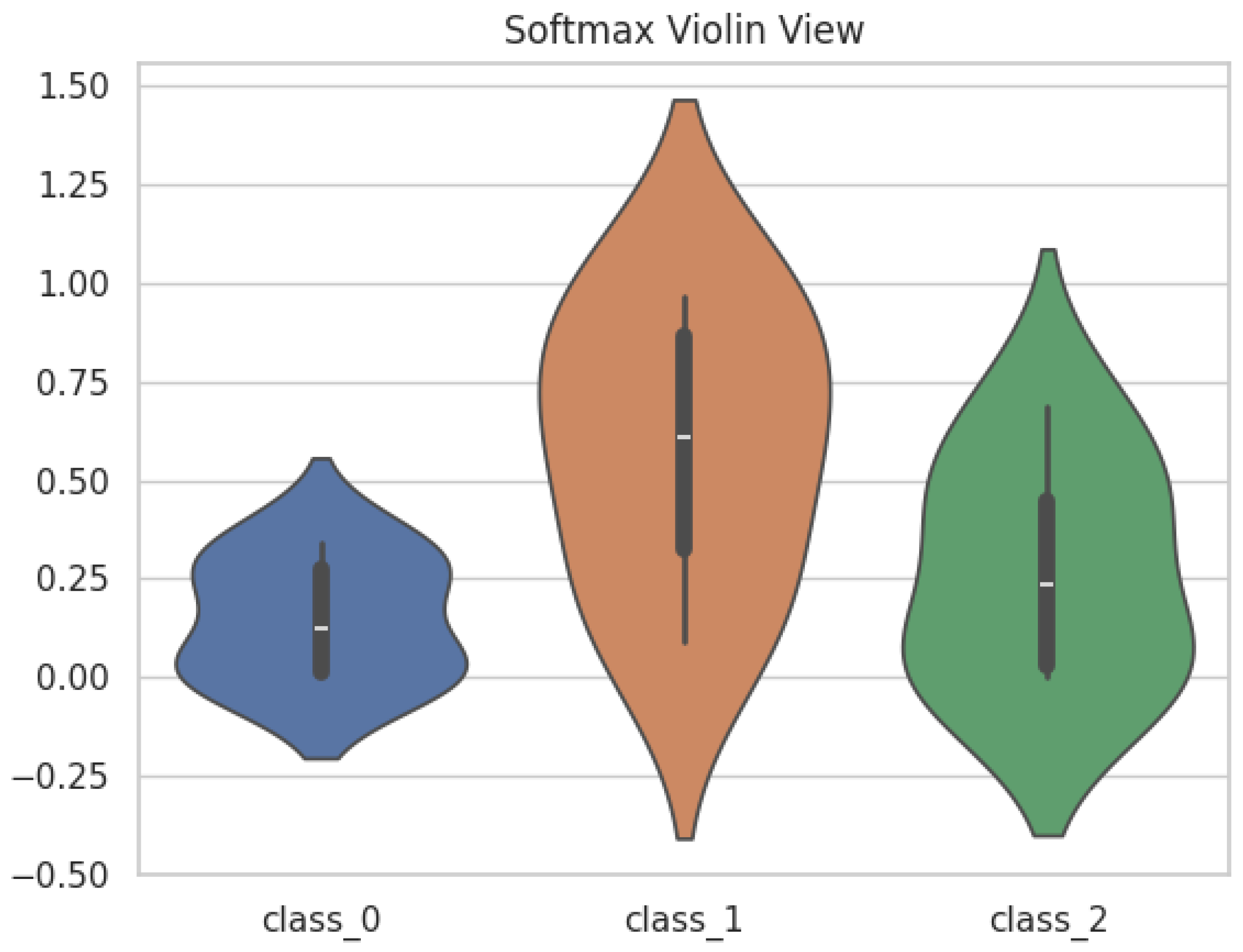
Figure 9 shows the predicted softmax confidence distributions for the three classification categories. In our label encoding, class_0 corresponds to Healthy, class_1 to Worn, and class_2 to Failed, which are the same three tool conditions reported in

Table 13. Class-wise classification, calibration and remaining useful life prediction performance on the test dataset.

Class	Prec.	Rec.	F1	AUC	AUPRC	RUL MAE (s)	ECE	Supp.
Healthy	0.89	0.91	0.90	0.95	0.95	2.1	0.03	1200
Worn	0.75	0.78	0.76	0.89	0.72	3.8	0.08	600
Failed	0.86	0.88	0.87	0.90	0.98	1.5	0.02	400

F1 is the harmonic mean of precision and recall. AUPRC = area under the precision–recall curve. RUL MAE = mean absolute error of remaining-useful-life predictions in seconds. ECE = expected calibration error. Supp. = number of test samples per class. All values are averaged across cross-validation folds.

. The softmax confidence score represents the normalized posterior probability assigned by the classifier to each class based on the network logits, and can be interpreted as the model’s degree of certainty in its prediction. As shown in Figure 9, the Healthy and Failed classes exhibit tight, high-confidence peaks, while the Worn class shows a broader distribution with greater overlap, reflecting its transitional and inherently ambiguous nature. This behavior indicates reasonable uncertainty calibration and supports the use of conservative decision thresholds for maintenance planning; for example, by flagging low-confidence Worn predictions for closer inspection rather than immediate intervention.

For quantitative performance, we report class-level precision, recall, and area under the ROC curve. Table 13 summarizes these metrics computed on the held-out test set and averaged across cross-validation folds so that the reported values reflect generalization performance.

Figure 8 and Figure 9 indicate stable convergence without late overfitting and confirm that the Worn state is the most challenging class, with lower and more dispersed confidence scores. Table 13 further confirms strong separation for the Healthy and Failed states, while the intermediate Worn condition remains less distinct. This suggests that most residual uncertainty is concentrated in the mid-degradation regime, and future work should target this class through finer-grained labeling, targeted augmentation, and improved uncertainty-aware modeling. While these results establish that the TCN learns a stable and accurate representation for joint health-state classification and RUL estimation, they do not yet explain how the model arrives at its decisions or which sensors and time regions dominate each prediction. To address this, the following subsection analyzes the internal attention patterns and feature attributions produced by the trained network, providing transparent, sensor-level and time-resolved explanations that connect the quantitative performance reported here to the underlying physical signals.

4.5. Attention Rollout, Saliency Analysis and Explainable Sensor Attribution

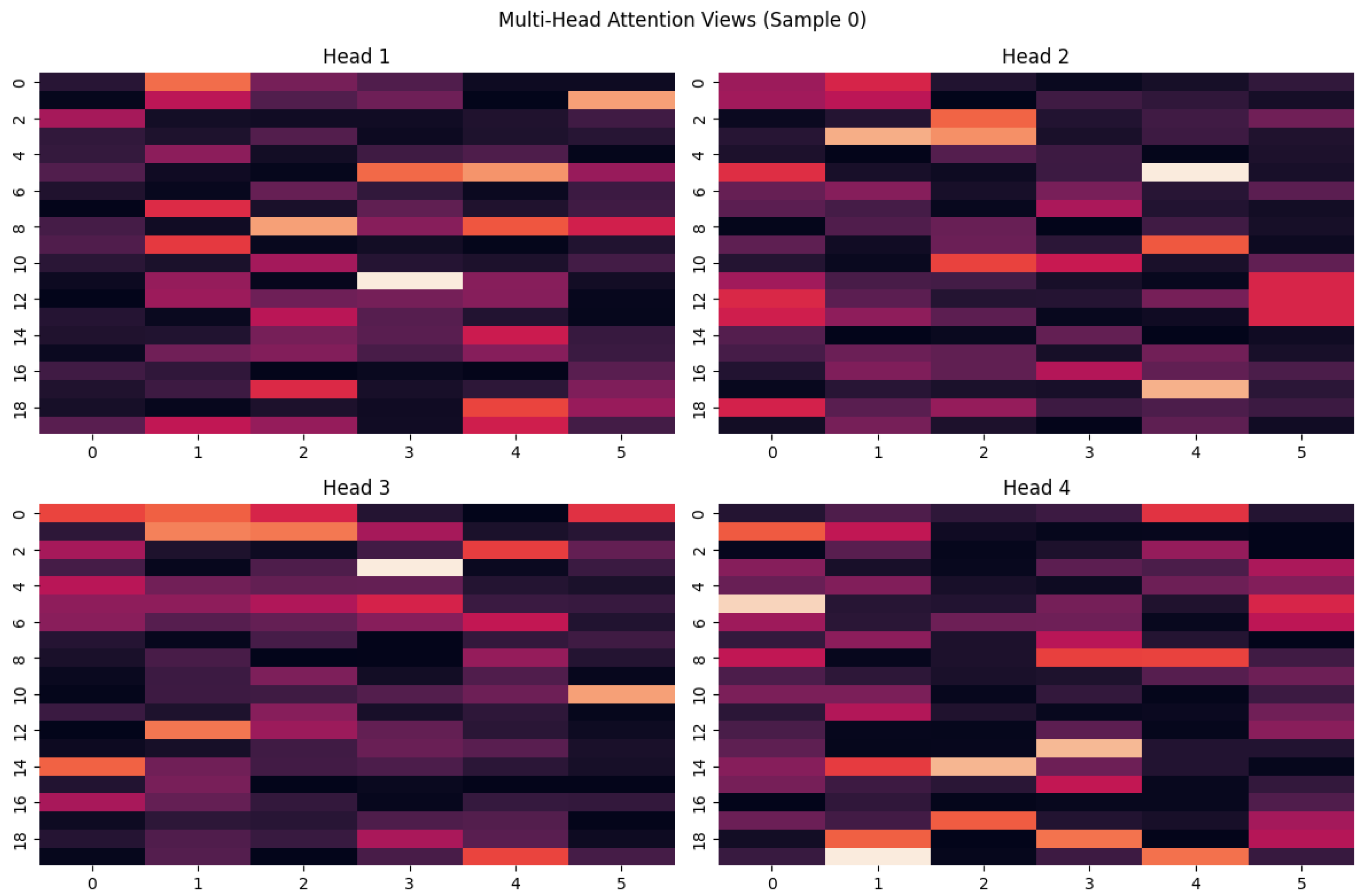
This subsection reports attention and saliency results that clarify which time regions and sensors drive TCN decisions. Figure 10 shows multi-head attention rollout, where some heads focus on short-term smcAC and smcDC fluctuations and others emphasize delayed vibration and acoustic responses. The complementary patterns indicate multi-scale temporal integration, reduced redundancy and improved robustness for health-state prediction.

Table 14. Combined explainability analyses linking signal dynamics, sensor behavior and learned model responses across machine health states.

Analysis	Key Focus	Primary Sensor	Derived Insight
Z-score heatmap	Normalized activation	smcAC, smcDC	Strong and coherent activations indicate dominant electrical health cues
Patch variability	Early variance	smcAC	High initial variance reflects process transients and degradation onset
RMS evolution	Amplitude growth	smcAC, smcDC	Progressive RMS increase tracks fatigue and load imbalance
Entropy trend	Signal complexity	AE_spindle	Entropy reduction signals loss of acoustic diversity with wear
Variance share	Energy dominance	smcAC, smcDC	Electrical load governs overall framework variability
SHAP failed	Feature impact	vib_table	Rising vibration energy reflects resonance near failure
SHAP worn	Feature impact	AE_spindle	Reduced acoustic activity aligns with partial tool dulling
SHAP healthy	Feature suppression	vib_table	Low vibration stabilizes framework and suppresses fault signatures

combines the signal behaviors and model explanation to show which sensor types are most important in detecting wear. Heatmaps of z scores and RMS trends highlight smcAC and smcDC as the main indicators across the full wear cycle. Analyses of patch variation and entropy show that signals change quickly at first and then lose complexity as the tool wears out. SHAP results point to vib_table as a key sign of failure, while the decreasing importance of AE_spindle matches the middle stages of wear. Together, these findings suggest that electrical changes happen before mechanical vibrations increase near the end of the tool’s life. These insights can guide better feature weighting, smarter alert limits and clearer feedback for operators to plan maintenance on time.

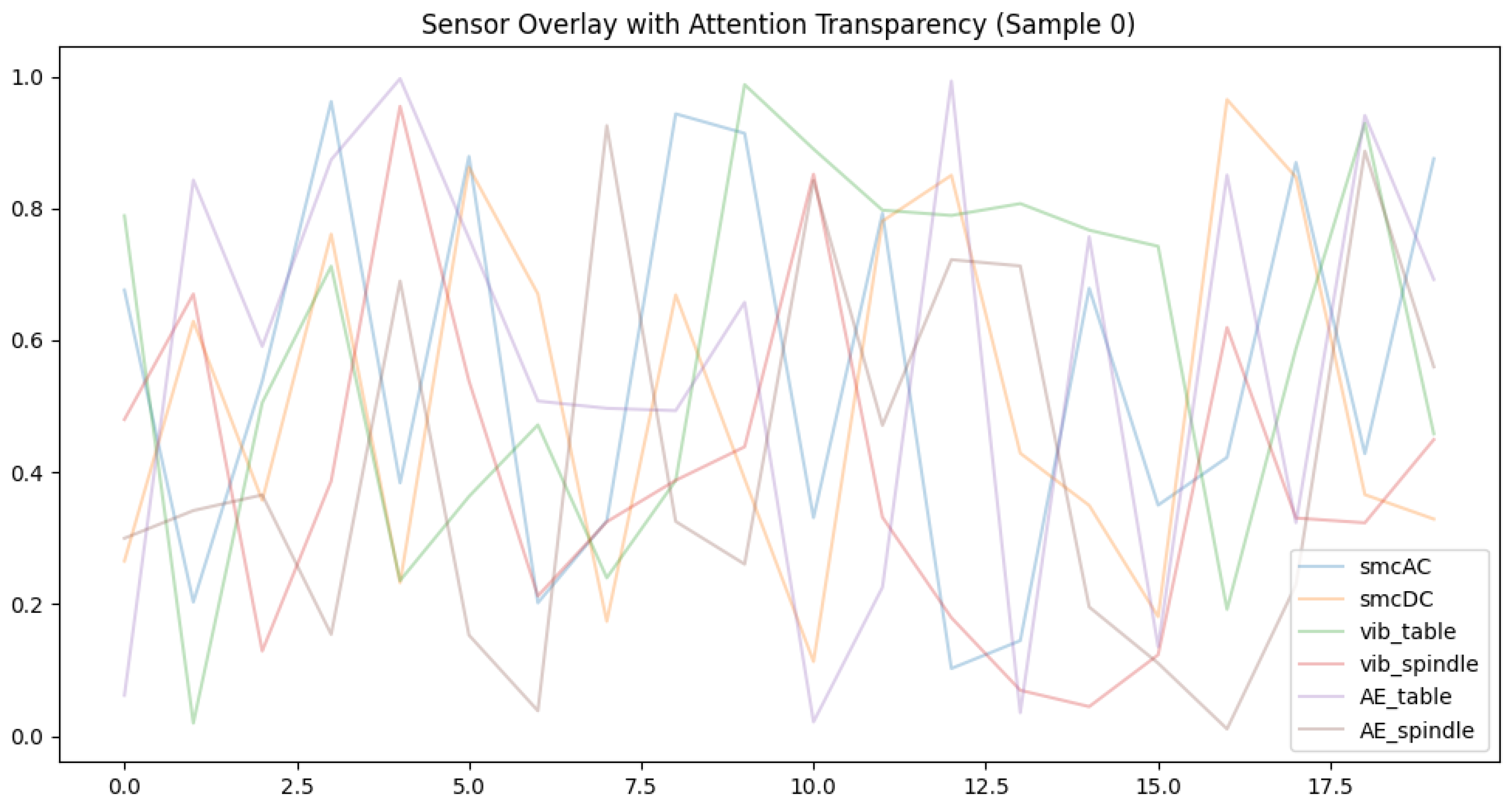
Figure 11 overlays attention across sensors to highlight decisive time regions. Shared peaks in smcAC, smcDC and vibration indicate consensus degradation events, while divergences show sensor-specific contributions or noise, improving traceability and trust.

Taken together, the attention rollouts, SHAP attributions, and sensor-level overlays provide a transparent link between the raw multi-sensor inputs, the learned multiscale representations, and the final health-state and RUL predictions. The deployment profiling further demonstrates that these explanations are obtained without compromising runtime or memory constraints. This closes the proposed pipeline end-to-end: from data preprocessing and feature construction, through temporal modeling, to auditable predictions and resource-aware deployment, satisfying both predictive performance and practical interpretability requirements for industrial use.

4.6. Attention-Based Interpretability and Deployment Profiling

To quantify these patterns and support feature weighting decisions, we report averaged attention weights for representative temporal patches alongside concise interpretability notes. The merged table below combines per-patch attention magnitudes with a short observation per sensor so that practitioners can quickly identify which channels and patches drive predictions.

Table 15. Patch-wise attention weights across sensors, highlighting dominant signals and their relative importance in fault detection.

Sensor	P0	P5	P10	P15	Rank	Key Observation
smcAC	0.012	0.014	0.010	0.011	2nd	Early electrical cues with mid-segment confirmation
smcDC	0.018	0.020	0.015	0.017	1st	Dominant attention aligned with current spikes and fault onset
vib_spindle	0.009	0.010	0.007	0.008	3rd	Mechanical response following electrical transients
AE_table	0.005	0.006	0.004	0.006	4th	Low attention; corroborative acoustic evidence

shows the numeric summary.

Figure 10 and Figure 11 show complementary attention patterns, with heads focusing on early electrical transients and later mechanical responses and consensus intervals supporting event triage. Table 15 ranks smcDC and smcAC as dominant, with vibration and acoustic supporting. Table 14 links RMS and complexity shifts to wear and flags vib_table for failure via SHAP.

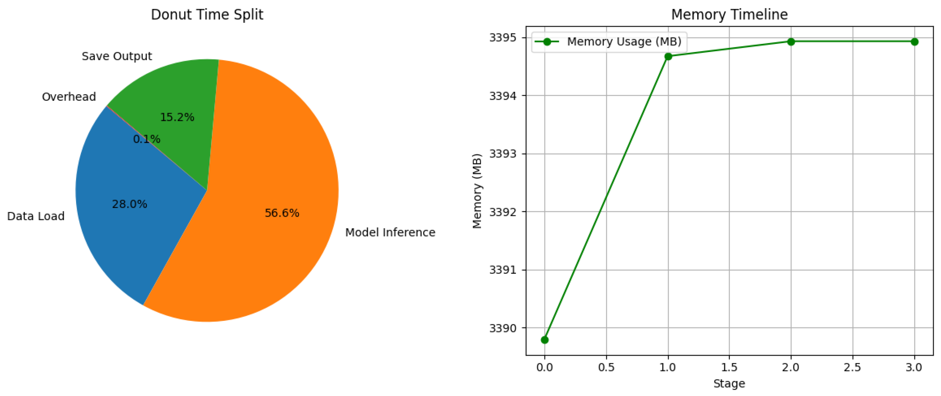
To evaluate deployment feasibility, detailed profiling was conducted to measure runtime latency, memory usage and CPU load across framework stages. These metrics assess whether the proposed TCN-based predictive maintenance framework can efficiently operate on edge or factory-level computing platforms. As shown in Figure 12, approximately 56% of the total runtime was spent on model inference, while data loading and output saving together accounted for 43%. This breakdown suggested that optimizing I/O operations could have further reduced latency and improved real-time performance in industrial systems.

Overall, the total runtime for one complete inference cycle is approximately 11 s. The framework maintains a consistent memory footprint and moderate CPU load throughout execution, confirming its suitability for real-time predictive maintenance on resource-constrained industrial or edge platforms.

5. Discussion and Comparison

Table 16. Performance, interpretability and edge suitability comparison of deep learning models for predictive maintenance across benchmark datasets.

Model	Dataset	Acc.	AUC	Lat.	Interp.	Edge	Remarks
CNN-LSTM [45]	NASA Milling/C-MAPSS	82	0.88	210	No	No	High temporal cost
Bi-LSTM [46]	NASA Milling	84	0.90	170	No	No	Good RUL; low interpret.
Transformer [47]	C-MAPSS	90	0.95	300+	Part.	No	High acc.; heavy compute
1D-CNN [48]	Milling	80	0.87	120	No	Yes	Light; lower precision
Proposed TCN (This work)	NASA Ames (Real)	87–89	0.89–0.96	89	High	High	High acc.; edge-ready

compares the proposed lightweight, interpretable TCN framework against common deep learning baselines on accuracy, AUC, latency, interpretability and edge suitability. The proposed method achieves strong accuracy with low inference time of about 89 ms and stable memory around 3.4 GB, supporting real-time deployment. Transformers slightly improve accuracy but require higher compute and memory, reducing edge feasibility. Combined SHAP attributions and attention visualizations provide transparent sensor-level reasoning, aligning predictive performance with practical maintenance decision support.

5.1. Predictive Performance, Calibration and Class Difficulty

Training dynamics indicate stable optimization and limited overfitting, with validation accuracy rising as both training and validation losses decrease in Figure 8. Confidence distributions in Figure 9 further show that the intermediate Worn state yields broader, lower-confidence predictions than Healthy and Failed, which is consistent with a gradual transition regime rather than a sharply separable condition. Quantitatively, Table 13 confirms strong discrimination for the extreme states and lower separability for Worn (for example, lower F1 and higher calibration error than the other classes), highlighting that most residual uncertainty concentrates in the mid-degradation stage. From a deployment perspective, this confidence structure supports conservative decision policies; for example, by treating low-confidence Worn predictions as candidates for closer inspection or continued monitoring rather than immediate maintenance action.

5.2. Explainability, Deployment Profile and Baseline Comparison

Attention and attribution results align with physically meaningful sensor roles. Multi-head attention rollout in Figure 10 shows distinct temporal focus patterns, with heads emphasizing early electrical fluctuations and delayed mechanical or acoustic responses, supporting multi-scale temporal integration. The composite transparency overlay in Figure 11 highlights shared attention peaks across key channels, improving traceability by separating consensus degradation intervals from sensor-specific contributions. Integrated interpretation in Table 14 links rising current-domain activation and RMS trends to wear progression and identifies vib_table as a salient failure indicator via SHAP, consistent with resonance growth near end-of-life.

Operational feasibility is supported by profiling results.

Table 17. End-to-end runtime, memory and CPU utilization profiling of the proposed predictive maintenance framework during inference.

Module	Time (s)	Mem. MB	CPU %	Role	Observation
Load CSV	1.2	3390	62.5	Input I O	Fast read with moderate CPU load
Preprocess	2.3	3394	75.3	Feature prep	CPU intensive due to filtering and scaling
Patchify	1.1	3395	53.1	Windowing	Stable memory and low overhead
TCN inference	4.7	3396	52.9	Core compute	Main latency contributor during prediction
Save output	1.8	3397	77.2	Output I O	Disk writes dominate CPU usage
Total or avg.	11.1	3394	64.2	End to end	Stable runtime and memory profile

shows a stable memory footprint around 3.39 GB and an end-to-end runtime of about 11 s, with inference as the main latency contributor and I/O-heavy stages dominating CPU utilization. In comparative terms, Table 16 indicates the proposed TCN achieves a strong accuracy-latency balance with inference around 89 ms and high interpretability and edge suitability, while transformer baselines can improve accuracy but require substantially higher compute and memory, reducing deployment practicality.

6. Conclusions and Future Work

This work presents a modular predictive maintenance framework that balances predictive performance, interpretability and operational practicality. Using the NASA Ames milling dataset, we developed a multiscale feature framework, carried out cross-sensor and spectral analyses and trained a temporal convolutional network that jointly performs tool health classification and remaining useful life estimation. Complementary interpretability tools, including attention rollouts and SHAP attributions, reveal consistent, physically plausible decision patterns and identify the sensors that provide the most diagnostic value. End-to-end profiling demonstrates that the framework meets realistic latency and memory constraints for deployment on standard industrial hardware. Taken together, the elements of preprocessing, feature design and transparent modeling produce a system that supports timely, explainable maintenance decisions and that can be integrated into existing production monitoring workflows. The clear mapping from sensor dynamics to model explanations increases operator trust and facilitates actionable interventions that reduce unplanned downtime. Future research should focus on reducing the model size and testing it on edge controllers to make sure it runs quickly and uses little memory, while still staying easy to understand. They should also explore adding online learning and uncertainty tracking and include more types of sensors through real-world testing to confirm the framework is reliable and brings clear value in practical use.

Future work will prioritize improving generalization and reliability under real shop-floor variability. First, cross-domain evaluation should be expanded beyond a single milling setup by training and testing across different machines, tools, materials, cutting parameters and sensor placements, using domain adaptation or feature normalization strategies to reduce distribution shift. Second, the intermediate Worn state can be strengthened through finer-grained labeling, temporal progression modeling and targeted augmentation that simulates gradual wear rather than abrupt faults. Finally, deployment studies should include on-device benchmarking on industrial edge hardware, streaming inference under throughput constraints and human-in-the-loop validation protocols that measure how explanations improve operator trust and maintenance outcomes.

References

1. Surucu, O.; Gadsden, S.A.; Yawney, J. Condition Monitoring using Machine Learning: A Review of Theory, Applications, and Recent Advances. Expert Syst. Appl. 2023, 221, 119738. [Google Scholar] [CrossRef]
2. Shokrani, A.; Dogan, H.; Burian, D.; Nwabueze, T.D.; Kolar, P.; Liao, Z.; Sadek, A.; Teti, R.; Wang, P.; Pavel, R.; et al. Sensors for in-process and on-machine monitoring of machining operations. CIRP J. Manuf. Sci. Technol. 2024, 51, 263–292. [Google Scholar] [CrossRef]
3. Thomas, D.; Weiss, B. Maintenance Costs and Advanced Maintenance Techniques in Manufacturing Machinery: Survey and Analysis. Int. J. Progn. Health Manag. 2021, 12, 10. [Google Scholar] [CrossRef] [PubMed Central]
4. Hermans, M.; Kozielski, M.; Michalak, M.; Szczyrba, K.; Wróbel, Ł.; Sikora, M. Sensor-Based Predictive Maintenance with Reduction of False Alarms-A Case Study in Heavy Industry. Sensors 2022, 22, 226. [Google Scholar] [CrossRef] [PubMed]
5. Wang, H.; Wang, S.; Sun, W.; Xiang, J. Multi-sensor signal fusion for tool wear condition monitoring using denoising transformer auto-encoder ResNet. J. Manuf. Process. 2024, 124, 1054–1064. [Google Scholar] [CrossRef]
6. Umar, M.; Siddique, M.F.; Kim, J.M. Burst-informed acoustic emission framework for explainable failure diagnosis in milling machines. Eng. Fail. Anal. 2026, 185, 110373. [Google Scholar] [CrossRef]
7. Hassan, I.U.; Panduru, K.; Walsh, J. Review of Data Processing Methods Used in Predictive Maintenance for Next Generation Heavy Machinery. Data 2024, 9, 69. [Google Scholar] [CrossRef]
8. Bouharrouti, N.E.; Morinigo-Sotelo, D.; Belahcen, A. Multi-Rate Vibration Signal Analysis for Bearing Fault Detection in Induction Machines Using Supervised Learning Classifiers. Machines 2024, 12, 17. [Google Scholar] [CrossRef]
9. Ahmad, J.; Iqbal, A.; Khan, A.; Al-Naeem, M. Engine Failure Prediction on Large-Scale CMAPSS Data Using Hybrid Feature Selection and Imbalance-Aware Learning. Comput. Mater. Contin. 2025. [Google Scholar] [CrossRef]
10. Sun, S.; Zhang, S.; Wang, W. A New Monitoring Technology for Bearing Fault Detection in High-Speed Trains. Sensors 2023, 23, 6392. [Google Scholar] [CrossRef]
11. Pei, D.; Yue, J.; Jiao, J. A Novel Method for Bearing Fault Diagnosis under Variable Speed Based on Envelope Spectrum Fault Characteristic Frequency Band Identification. Sensors 2023, 23, 4338. [Google Scholar] [CrossRef] [PubMed]
12. Jaros, R.; Byrtus, R.; Dohnal, J.; Danys, L.; Baros, J.; Koziorek, J.; Zmij, P.; Martinek, R. Advanced Signal Processing Methods for Condition Monitoring. Arch. Comput. Methods Eng. 2022, 30, 1553–1577. [Google Scholar] [CrossRef]
13. Jimenez-Cortadi, A.; Irigoien, I.; Boto, F.; Sierra, B.; Rodriguez, G. Predictive Maintenance on the Machining Process and Machine Tool. Appl. Sci. 2020, 10, 224. [Google Scholar] [CrossRef]
14. Hector, I.; Panjanathan, R. Predictive maintenance in Industry 4.0: A survey of planning models and machine learning techniques. PeerJ Comput. Sci. 2024, 10, e2016. [Google Scholar] [CrossRef] [PubMed]
15. Wang, H. Remaining Useful Life Prediction Based on Improved Temporal Convolutional Network. Front. Energy Res. 2020, 8, 584463. [Google Scholar] [CrossRef]
16. Siddique, M.F.; Zaman, W.; Umar, M.; Kim, J.Y.; Kim, J.M. A Hybrid Deep Learning Framework for Fault Diagnosis in Milling Machines. Sensors 2025, 25, 5866. [Google Scholar] [CrossRef]
17. Khan, U. A Comprehensive Survey on Deep Learning-based Predictive Maintenance. ACM Trans. Embed. Comput. Syst. 2025. [Google Scholar] [CrossRef]
18. Nor, A.K.M.; Pedapati, S.R.; Muhammad, M.; Leiva, V. Overview of Explainable Artificial Intelligence for Prognostic and Health Management of Industrial Assets based on PRISMA. Sensors 2021, 21, 8020. [Google Scholar] [CrossRef]
19. Bayram, F.; Ahmed, B.S. A domain-region based evaluation of ML performance robustness to covariate shift. Neural Comput. Appl. 2023, 35, 17555–17577. [Google Scholar] [CrossRef]
20. Molęda, M.; Małysiak-Mrozek, B.; Ding, W.; Sunderam, V.; Mrozek, D. From Corrective to Predictive Maintenance—A Review of Maintenance Approaches for the Power Industry. Sensors 2023, 23, 5970. [Google Scholar] [CrossRef]
21. Idowu, S.; Osman, O.; Strüber, D.; Berger, T. Machine learning experiment management tools: A mixed-methods empirical study. Empir. Softw. Eng. 2024, 29, 74. [Google Scholar] [CrossRef]
22. Cao, Y.; Ding, Y.; Jia, M.; Tian, R. A novel temporal convolutional network with residual self-attention mechanism for remaining useful life prediction of rolling bearings. Reliab. Eng. Syst. Saf. 2021, 215, 107813. [Google Scholar] [CrossRef]
23. Nunes, P.; Rocha, E.; Santos, J.; Antunes, R. Challenges in predictive maintenance—A review. CIRP J. Manuf. Sci. Technol. 2023, 40, 53–67. [Google Scholar] [CrossRef]
24. Lara-Benítez, P.; Carranza-García, M.; Luna-Romera, J.M.; Riquelme, J.C. Temporal convolutional networks applied to energy-related time series forecasting. Appl. Sci. 2020, 10, 2322. [Google Scholar] [CrossRef]
25. Bucay-Valdiviezo, J.; Escudero-Villa, P.; Paredes-Fierro, J.; Ayala-Chauvin, M. Leveraging Classical Statistical Methods for Sustainable Maintenance in Automotive Assembly Equipment. Sustainability 2023, 15, 15604. [Google Scholar] [CrossRef]
26. Souza, M.L.H.; da Costa, C.A.; de Oliveira Ramos, G. A machine-learning based data-oriented pipeline for Prognosis and Health Management Systems. Comput. Ind. 2023, 148, 103903. [Google Scholar] [CrossRef]
27. Mienye, I.D.; Swart, T.G.; Obaido, G. Recurrent Neural Networks: A Comprehensive Review of Architectures, Variants and Applications. Information 2024, 15, 517. [Google Scholar] [CrossRef]
28. Song, X.; Deng, L.; Wang, H.; Zhang, Y.; He, Y.; Cao, W. Deep learning-based time series forecasting. Artif. Intell. Rev. 2024, 58, 23. [Google Scholar] [CrossRef]
29. Wei, X.; Wang, Z. TCN-attention-HAR: Human activity recognition based on attention mechanism time convolutional network. Sci. Rep. 2024, 14, 7414. [Google Scholar] [CrossRef]
30. Bednarski, B.P.; Singh, A.D.; Zhang, W.; Jones, W.M.; Naeim, A.; Ramezani, R. Temporal convolutional networks and data rebalancing for clinical length of stay and mortality prediction. Sci. Rep. 2022, 12, 21247. [Google Scholar] [CrossRef] [PubMed]
31. Nan, M.; Trăscău, M.; Florea, A.M.; Iacob, C.C. Comparison between Recurrent Networks and Temporal Convolutional Networks Approaches for Skeleton-Based Action Recognition. Sensors 2021, 21, 2051. [Google Scholar] [CrossRef] [PubMed]
32. Singh, V.; Singh, S.K. A separable temporal convolutional networks based deep learning technique for discovering antiviral medicines. Sci. Rep. 2023, 13, 13722. [Google Scholar] [CrossRef]
33. Hekman, S.; Brock, M.; Khan, M.A.A.H.; Zhang, X. Comparison of Long Short-Term Memory Networks and Temporal Convolutional Networks for Sentiment Analysis. In Proceedings of the 2023 ACM Southeast Conference; Association for Computing Machinery: New York, NY, USA, 2023; pp. 2–9. [Google Scholar] [CrossRef]
34. Zhang, C.; Zeng, M.; Fan, J.; Li, X. Application of Residual Structure Time Convolutional Network Based on Attention Mechanism in Remaining Useful Life Interval Prediction of Bearings. Sensors 2024, 24, 4132. [Google Scholar] [CrossRef]
35. Zhang, Q.; Liu, Q.; Ye, Q. An attention-based temporal convolutional network method for predicting remaining useful life of aero-engine. Eng. Appl. Artif. Intell. 2024, 127, 107241. [Google Scholar] [CrossRef]
36. NASA Prognostics Center of Excellence. C-MAPSS Aircraft Engine Simulator Data. 2025. Available online: https://data.nasa.gov/dataset/c-mapss-aircraft-engine-simulator-data (accessed on 17 June 2025).
37. WangBiaoXJTU. XJTU-SY Bearing Datasets Repository. 2024. Available online: https://github.com/WangBiaoXJTU/xjtu-sy-bearing-datasets (accessed on 17 June 2025).
38. Figshare. Milling Data Set Prognostic Data. 2024. Available online: https://figshare.com/articles/dataset/Milling_dataset/27323346 (accessed on 17 June 2025).
39. Li, C.; Li, S.; Feng, Y.; Gryllias, K.; Gu, F.; Pecht, M. Small data challenges for intelligent prognostics and health management: A review. Artif. Intell. Rev. 2024, 57, 214. [Google Scholar] [CrossRef]
40. Kozielski, M. Contextual Explanations for Decision Support in Predictive Maintenance. Appl. Sci. 2023, 13, 10068. [Google Scholar] [CrossRef]
41. Bala, A.; Rashid, R.Z.J.A.; Ismail, I.; Oliva, D.; Muhammad, N.; Sait, S.M.; Al-Utaibi, K.A.; Amosa, T.I.; Memon, K.A. Artificial intelligence and edge computing for machine maintenance-review. Artif. Intell. Rev. 2024, 57, 119. [Google Scholar] [CrossRef]
42. Mittal, P. A comprehensive survey of deep learning-based lightweight object detection models for edge devices. Artif. Intell. Rev. 2024, 57, 242. [Google Scholar] [CrossRef]
43. Teubert, C. Milling Wear. 2022. Available online: https://data.nasa.gov/dataset/milling-wear (accessed on 17 June 2025).
44. Tyagi, V. NASA Milling Dataset: Prognostic Dataset for Predictive/Preventive Maintenance. 2019. Available online: https://www.kaggle.com/datasets/vinayak123tyagi/milling-data-set-prognostic-data (accessed on 17 June 2025).
45. Saxena, A.; Goebel, K.; Simon, D.; Eklund, N. Damage Propagation Modeling for Aircraft Engine Run-to-Failure Simulation. In Proceedings of the 2008 International Conference on Prognostics and Health Management, Denver, CO, USA, 6–9 October 2008; IEEE: Piscataway, NJ, USA, 2008. [Google Scholar] [CrossRef]
46. Zheng, S.; Ristovski, K.; Farahat, A.; Gupta, C. Long short-term memory network for remaining useful life estimation. In Proceedings of the 2017 IEEE International Conference on Prognostics and Health Management (ICPHM), Dallas, TX, USA, 19–21 June 2017; IEEE: Piscataway, NJ, USA, 2017; pp. 88–95. [Google Scholar] [CrossRef]
47. Chen, L.; Gao, Y.; Dui, H.; Xing, L. Importance Measure-Based Maintenance Optimization Strategy for Pod Slewing System. Reliab. Eng. Syst. Saf. 2021, 216, 108001. [Google Scholar] [CrossRef]
48. Susto, G.A.; Schirru, A.; Pampuri, S.; McLoone, S.; Beghi, A. Machine learning for predictive maintenance: A multiple classifier approach. IEEE Trans. Ind. Inform. 2015, 11, 812–820. [Google Scholar] [CrossRef]
Figure 1. Predictive maintenance architecture for a CNC machine tool, showing how sensor signals flow through acquisition, the PLC and NC control unit, triggering, storage, and operator feedback. The diagram emphasizes that diagnosis quality is set upstream by synchronized sensing and event-driven recording. Adapted and enhanced from Jimenez-Cortadi et al. [13], licensed under CC BY 4.0.
Machines 14 00164 g001
Figure 2. End- to-end modular framework from raw multi-sensor streams to TCN-based predictions. It summarizes the main stages for preprocessing, multiscale feature construction, training, evaluation, and interpretation within a single reproducible flow.
Machines 14 00164 g002
Figure 3. Framework overview linking raw sensor acquisition to feature fusion, TCN inference, and dual outputs for health state classification and remaining useful life estimation, with attention and SHAP-based explanations generated alongside predictions.
Machines 14 00164 g003
Figure 4. Deployment sketch illustrating a conceptual multi-machine scenario in which multiple machines stream sensor data to a central TCN-based prediction block, with operator-facing outputs including attention heatmaps, SHAP values, and remaining useful life trends.
Machines 14 00164 g004
Figure 5. Parallel coordinates comparison of RMS feature magnitudes across sensors for short, medium, and long window scales. Each polyline represents the RMS feature vector of one windowed sample, and overlapping trajectories are intentional, reflecting natural variability across samples rather than obscuring scientific interpretation. Colors encode the window scale, with red indicating short windows, orange indicating medium windows, and gray indicating long windows.
Machines 14 00164 g005
Figure 6. Correlation heatmap for the final time window, showing modality coupling patterns across current, vibration, and acoustic channels. The strongest relationship appears between AE table and AE spindle, while smcAC and smcDC exhibit moderate association.
Machines 14 00164 g006
Figure 7. Residual overlay across all sensor channels for a representative run, illustrating how deviations from the reference signal evolve over time. The current channels show the largest excursions, supporting their prioritization in residual based sensor ranking.
Machines 14 00164 g007
Figure 8. Learning curves over epochs, showing validation accuracy rising as validation loss decreases. The trends indicate stable convergence without abrupt divergence during training.
Machines 14 00164 g008
Figure 9. Violin plot of predicted softmax confidence by class, where class_0 = Healthy, class_1 = Worn, and class_2 = Failed. The plot shows tighter confidence distributions for the extreme states and broader uncertainty for the intermediate Worn state.
Machines 14 00164 g009
Figure 10. Multi-head attention heatmaps for a representative sample, illustrating how different attention heads emphasize different time steps and feature groups. Color intensity encodes the normalized attention weight assigned by each head, with darker colors indicating lower attention contribution and brighter colors indicating higher attention contribution. The diversity across heads reflects complementary temporal cues and multi-scale dependencies exploited by the model.
Machines 14 00164 g010
Figure 11. Attention transparency overlay across sensor channels for a representative sample. Each curve shows the normalized attention-weighted contribution of one sensor over time. Overlapping trajectories are intentional and illustrate concurrent sensor influence rather than obscuring information; dominant sensors and temporal emphasis are interpreted by relative magnitude and consistent trends rather than isolated peaks.
Machines 14 00164 g011
Figure 12. Runtime and memory profiling summary, decomposing end-to-end time into data loading, inference, and overhead, and reporting the corresponding peak memory trajectory during execution.
Machines 14 00164 g012