A Real-Time Obstacle Detection Framework for Gantry Cranes Using Attention-Augmented YOLOv5s and EIoU Optimization

Abstract

To meet the need for efficient and precise detection of people and obstacles in the actual operating environment of a gantry crane, a detection model based on an improved YOLOv5s was proposed which incorporates the parameter-free SimAM attention mechanism to enhance obstacle feature extraction capabilities, employs the EIoU loss function to optimize bounding box regression accuracy, and utilizes preprocessing techniques to improve input image quality. Training experiments on humans and simple simulated obstacles demonstrate that the improved model achieves significantly higher recognition accuracy and speed compared to the original YOLOv5 model. The improved model was applied to the recognition experiments of reducer obstacles under varying sizes, visibility levels, and distance conditions, and the comparative experiments were conducted with mainstream YOLO models, as well as different attention mechanisms and loss functions. The results show that the mAP@0.5 of the improved model achieves 0.884 with superior recognition performance and used lower computational resource requirements, providing a reliable solution for real-time obstacle detection in crane operation scenarios.

1. Introduction

Gantry cranes, as critical equipment in national economic development, are widely used in various indoor industrial settings such as indoor port warehouses, indoor cargo yard transfer centers, and supporting facilities for water conservancy projects. However, operating in complex and dynamically changing environments, crane safety faces severe challenges [1,2,3,4]. Traditional obstacle detection systems primarily rely on ultrasonic sensors, LiDAR, or rule-based algorithms. These technologies exhibit significant limitations in terms of sensing range, hardware costs, and adaptability to sudden dynamic obstacles such as moving personnel or barriers. Moreover, the most existing obstacle detection methods rely on centralized training processes, which may constrain their scalability and robustness in complex industrial environments [5]. This can lead to collision incidents, posing serious threats to personnel safety and equipment integrity. With the deepening advancement of Industry 4.0 and smart manufacturing, the transformation and upgrading of cranes toward automation and unmanned operation have become an inevitable trend. This transition is driving the application of visual recognition technology in obstacle detection [6,7,8,9,10].

In recent years, deep learning-based object detection methods have achieved remarkable progress. Akber [11] employed a deep neural network with an attention mechanism optimized by a tree-structured Parzen estimator to predict load movement conditions during tower crane dynamic operations. Zhao et al. [12] proposed a deep learning-based autonomous exploration method for UAVs. By integrating a hybrid action space combining positional and yaw actions, it addresses the UAV’s field-of-view limitations. With the rapid advancement of computer vision and deep learning technologies, vision-based automatic obstacle detection offers new technical pathways to enhance crane operation safety and automation levels [13]. Among these, the single-stage object detection algorithm YOLO series is highly favored for its excellent balance between speed and accuracy. Considering the complexity, dynamism, and stringent real-time requirements of crane operation scenarios, selecting an appropriate obstacle detection model is crucial [14]. Peng et al. [15] developed an emergency obstacle avoidance system for sugarcane harvesters based on the YOLOv5s algorithm. This addresses blade damage caused by collisions between the base cutter and obstacles during harvesting. The system incorporates attention mechanisms and lightweight network design. The improved model was deployed on a Raspberry Pi to enable real-time obstacle detection and avoidance control.

However, current research specifically targeting human and obstacle detection in the complex operational scenarios of gantry cranes remains relatively scarce. Existing detection models, in their pursuit of capturing high-order features and multi-scale target robustness, often suffer from numerous model parameters and high computational complexity. This makes it challenging to support real-time inference for complex models, leading to detection delays and failing to meet the higher efficiency requirements for obstacle detection in gantry cranes. Therefore, this paper proposes an improved YOLOv5s model and algorithm incorporating the SimAM attention mechanism. Input image quality is enhanced through preprocessing techniques, and the improved model’s recognition accuracy and efficiency are validated through experiments identifying people and simple simulated obstacles. Subsequently, this model is applied to recognition experiments involving actual reducer obstacles of varying sizes under different operating conditions to verify its performance in identifying real-world obstacles. This work provides new insights and methodologies for person and obstacle recognition in crane operation scenarios.

2. Methods

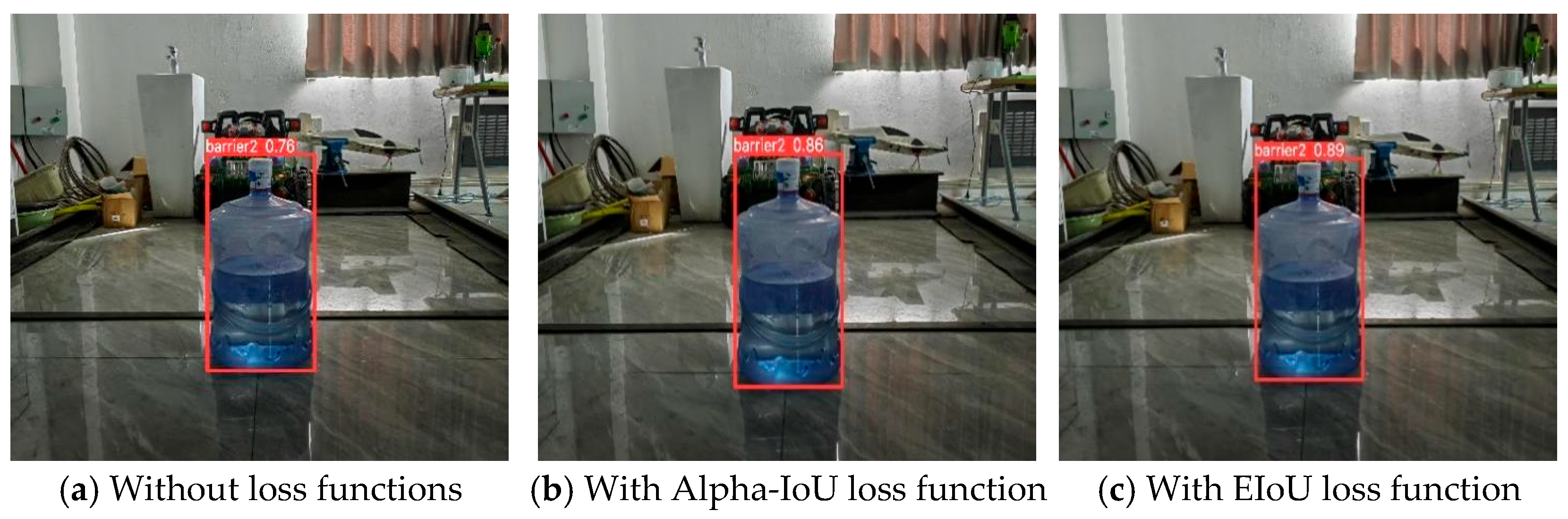
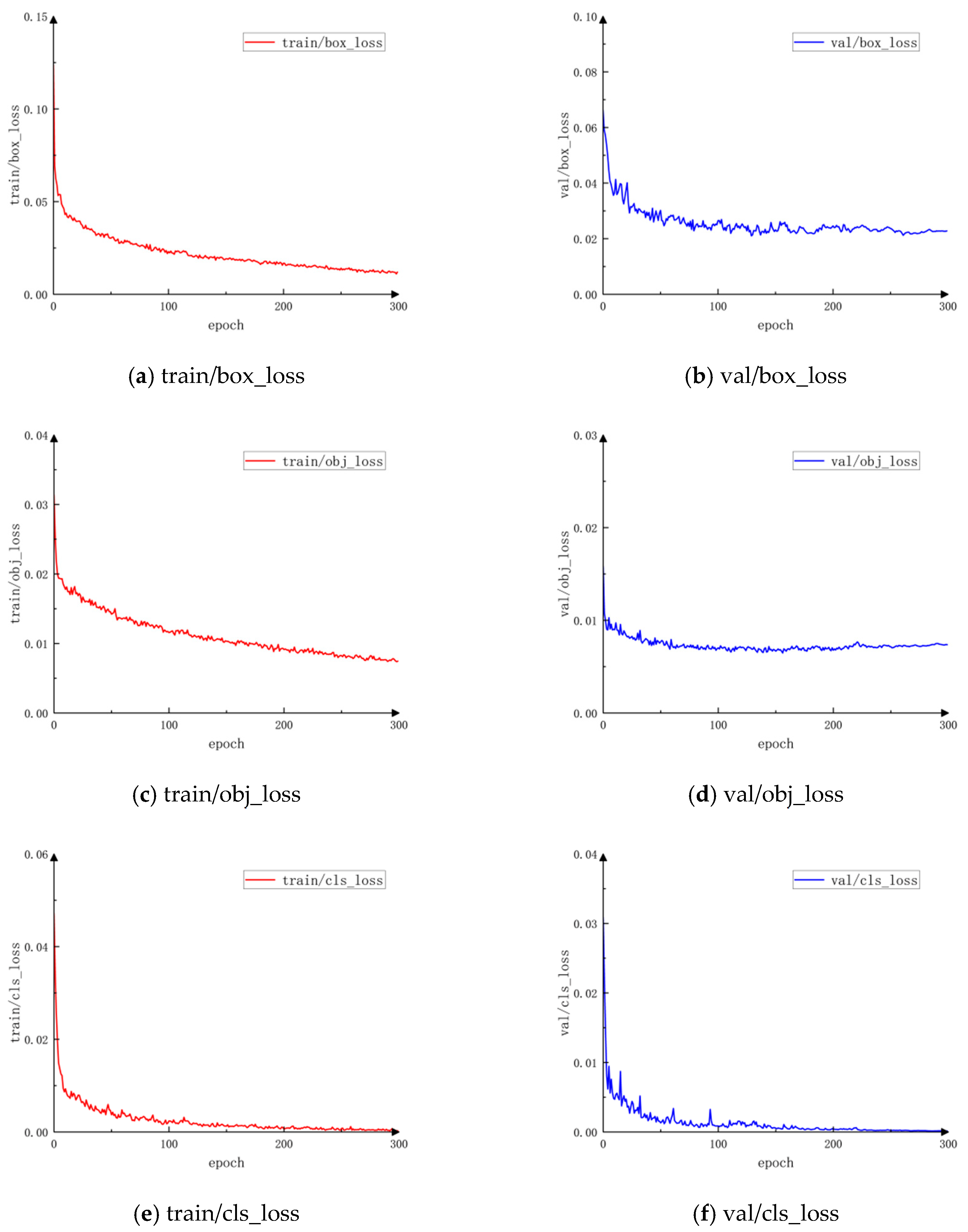
This chapter aims to develop a high-precision obstacle detection model tailored for the complex operational environment of cranes. Addressing common industrial challenges such as uneven lighting, noise interference, and significant variations in obstacle scale, an enhanced YOLOv5 model is proposed. Using the lightweight YOLOv5s as the baseline framework, image enhancement and denoising preprocessing techniques are introduced at the data input stage. Subsequently, the SimAM parameter-free attention mechanism is embedded at the feature extraction stage of the network and replaces the original loss function with EIoU at the output stage. These optimizations collectively define the architecture of the enhanced model.

2.1. YOLOv5 Model

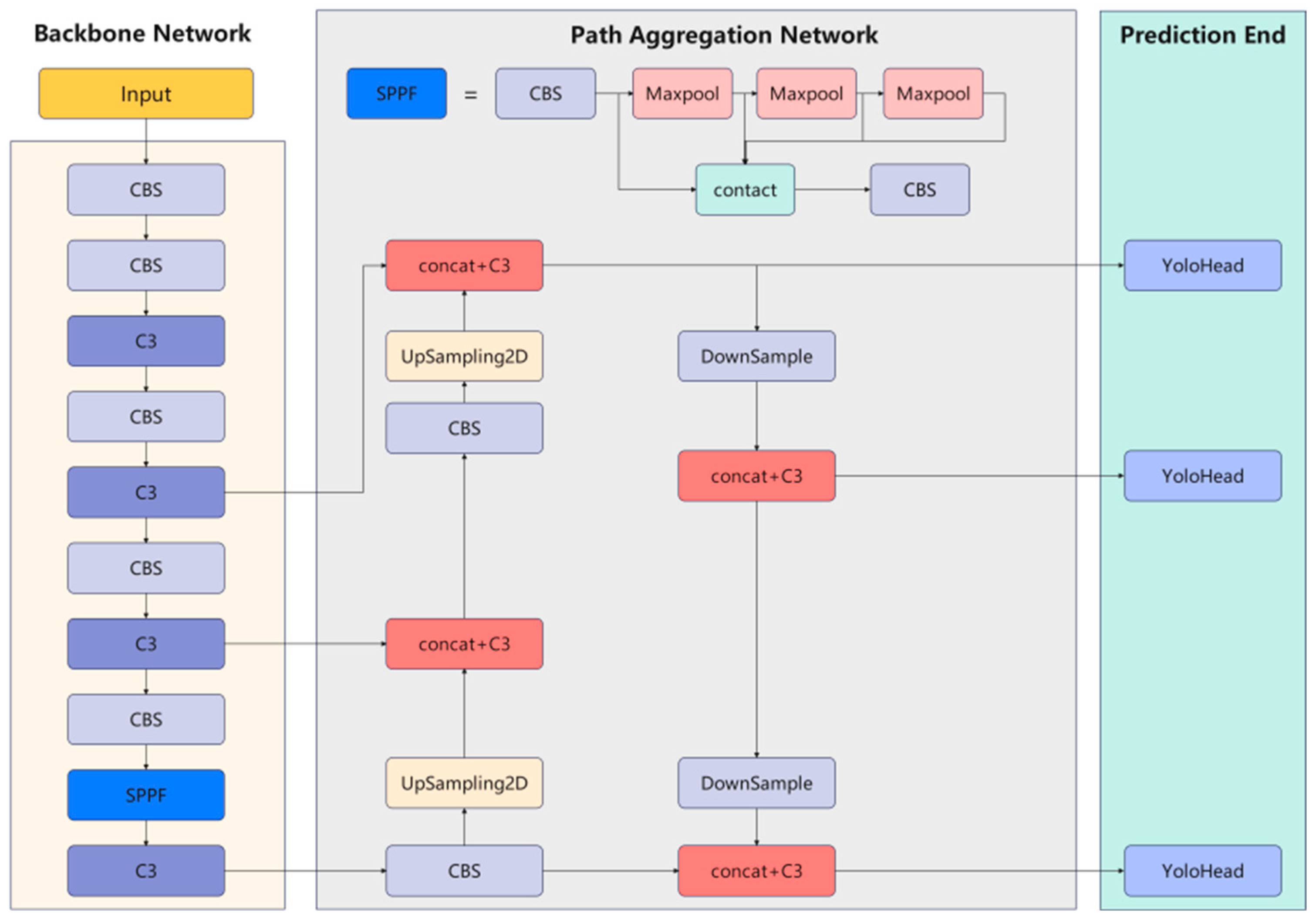
In the field of crane obstacle detection, the YOLO algorithm introduces fully convolutional neural networks, transforming object detection into a regression problem and significantly improving detection speed. YOLOv5 is an efficient object detection framework developed by Ultralytics (Frederick, MD, USA), designed based on the PyTorch (Version: PyTorch 1.11.0) deep learning library for easy deployment across various devices [16,17,18]. 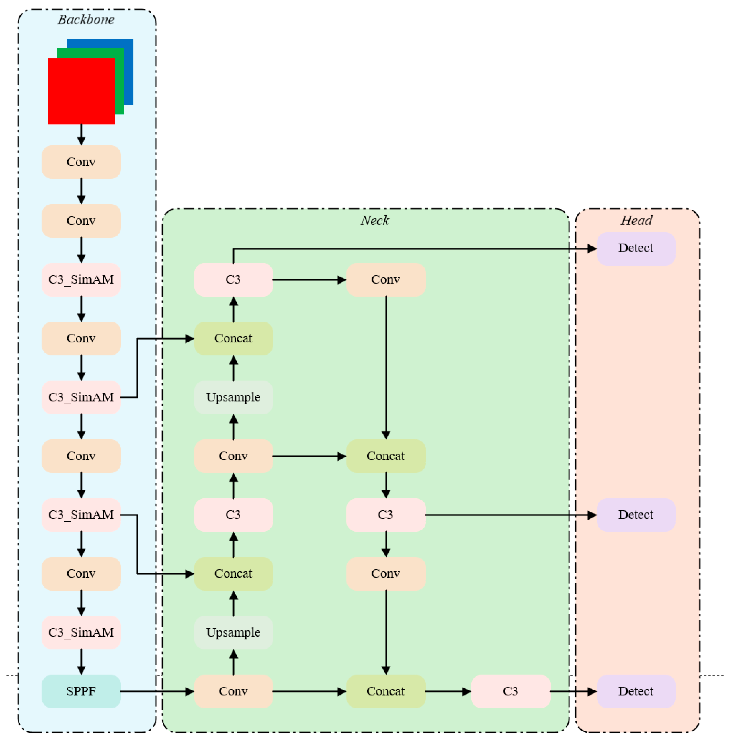The YOLOv5 network architecture comprises three main components: the backbone network, the feature fusion network, and the head network, as illustrated in Figure 1 using Visio. The backbone network primarily consists of CBS, C3, and SPFF modules. The CBS module first performs 2D convolutions, followed by a Batch Normalization (BN) layer that accelerates model training convergence through normalization. The SiLU activation function introduces nonlinear features to enhance the network’s fitting capability. The main branch of the C3 module extracts deep features through multiple Bottleneck layers, while the residual branch directly passes raw features. Features from both branches are ultimately concatenated and fused. SPFF performs pooling operations on input features across multiple scales, then concatenates the pooled results from these scales. The feature fusion network bidirectionally concatenates shallow detail features and deep semantic features from the backbone network, enabling features to simultaneously carry both detail and semantic information. The head network is used to detect object locations and categories.

2.2. Preprocessing Optimization

The crane operation scenario features a complex background, and the edges of obstacles are often blurred due to factors such as lighting variations and shooting distances. Additionally, images captured in industrial environments are susceptible to Gaussian noise and sensor thermal noise contamination. Meanwhile, the crane operation scenarios at night or in poorly lit workshops face dynamically changing lighting conditions, all of which can compromise the accuracy of subsequent target detection.

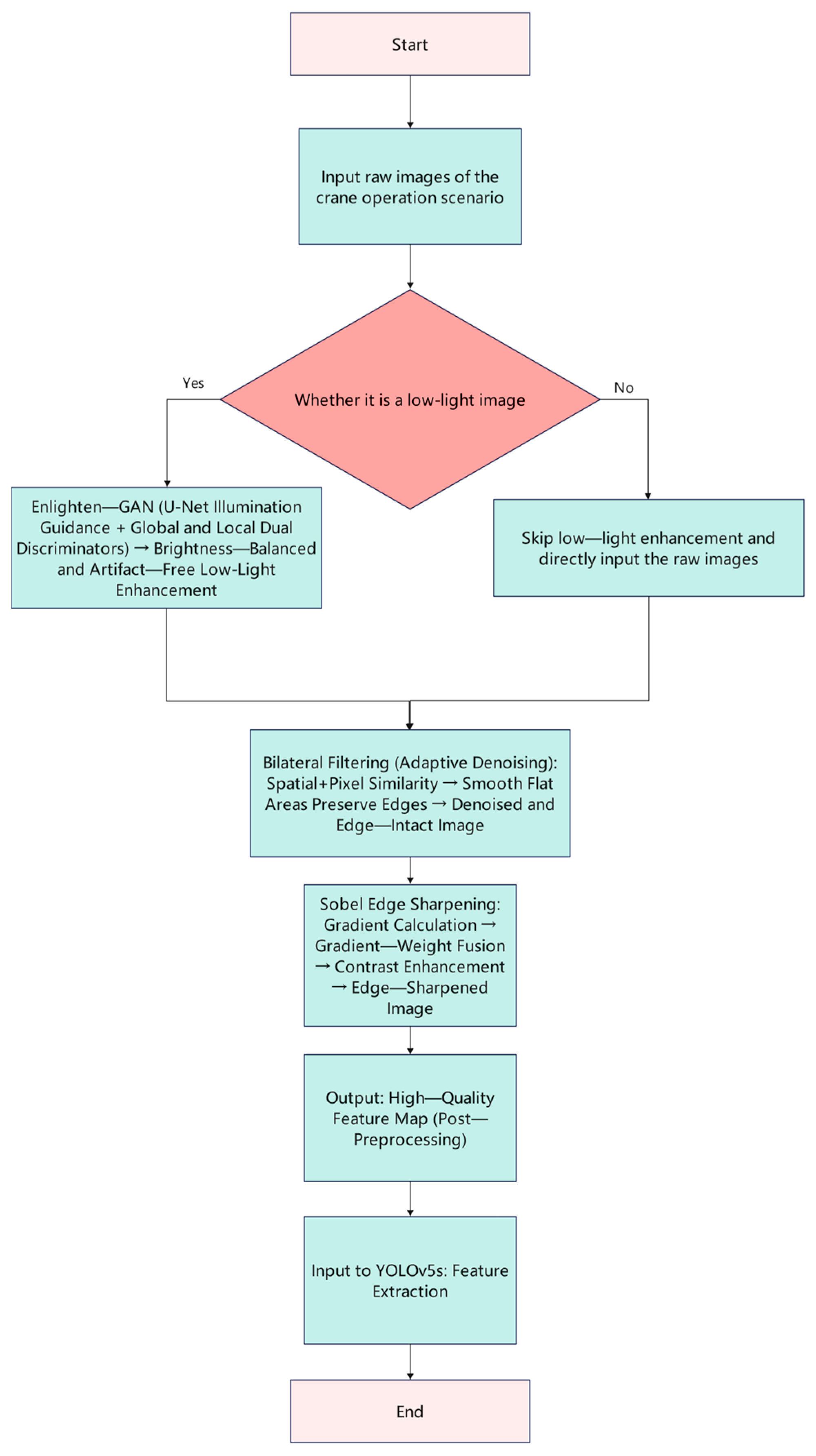
To enhance the model’s ability to extract features of key obstacle contours, this study proposes a multi-stage image preprocessing pipeline. Firstly, the Sobel operator is employed for image sharpening. Compared with other edge detection operators, the Sobel operator incorporates a weighted smoothing mechanism, which can effectively suppress noise amplification while calculating horizontal and vertical gradients [19,20,21]. By integrating local gradient information with neighborhood pixel weights, this method significantly enhances the boundary contrast between obstacles and the background, facilitating the detection network to capture the geometric structure information of objects. Secondly, the bilateral filtering algorithm is selected for adaptive denoising. Through nonlinear combination, this algorithm simultaneously considers the spatial proximity and pixel value similarity of pixels. Its core advantage lies in its ability to adaptively smooth textures in flat regions while preserving edge information with drastic intensity changes, thereby effectively removing environmental noise while maximizing the integrity of obstacle structural features. This avoids the edge blurring problem caused by traditional linear filtering and is more suitable for small target detection requirements [22,23]. Finally, the unsupervised learning-based Enlighten-GAN network is introduced for low-light image enhancement. Unlike traditional methods that rely on paired training data, this network adopts a generative adversarial network architecture, realizing adaptive enhancement without paired data through a U-Net-based generator and a global–local dual discriminator structure [24,25].

The generator guides the illumination distribution using a self-attention mechanism, as shown in Figure 2, while the discriminator ensures that the enhanced images have balanced overall brightness without local overexposure or artifact generation through adversarial training on global and locally cropped patches. After processing through the aforementioned preprocessing pipeline, the clarity and contrast of the input images are significantly improved, noise is effectively suppressed, and edge features are preserved intact, providing high-quality feature map support for subsequent feature extraction by the YOLOv5s model.

2.3. Introduction of Attention Mechanisms

Attention mechanisms are inspired by human characteristics, mimicking our ability to focus on the subject within an image while paying little attention to its background. Introducing attention mechanisms allows the model to concentrate more on the objects to be identified, thereby optimizing the network’s detection performance.

Current mainstream attention mechanisms include self-attention, multi-head attention, and convolutional attention. Among these, self-attention is the most commonly used, generating attention weights by calculating correlations between different positions in the input data. In visual model networks, adding attention mechanisms assigns corresponding weights to different regions within an image [26]. Regions with higher weights receive greater attention during model training and detection, while regions with lower weights receive less attention. Based on this principle, visual model networks can be optimized, improving performance metrics such as mAP@0.5 and precision.

(1)

SE Attention Mechanism

Global average pooling compresses each channel of the feature map into a single value. Two fully connected layers then learn the weights between channels—the attention scores—which are finally mapped between 0 and 1 via a Sigmoid function. These scores adjust the channel responses of the original feature map.

For an input feature map $\mathit{F}\in {\mathit{R}}^{\mathit{C}\times \mathit{H}\times \mathit{W}}$, the SE module first obtains $\mathit{z}\in {\mathit{R}}^{\mathit{C}\times 1\times 1}$ via global average pooling. It then derives weights $\mathit{s}\in {\mathit{R}}^{\mathit{C}\times 1\times 1}$ through a fully connected layer and activation function. The computation process can be expressed as follows:

$$z_c = \frac{1}{H\times W}{\sum }_{i=1}^H{\sum }_{j=1}^W{F}_c(i,j)$$

(1)

$$s=\sigma (g(z,W))$$

(2)

where $\mathbf{g}$ denotes the fully connected layer, $\mathit{\sigma }$ represents the Sigmoid activation function, and $W$ signifies the weight parameters of the fully connected layer. Finally, the learned weights $\mathit{s}$ are multiplied channel-wise with the original feature map $\mathit{F}$ to obtain the weighted feature map, thereby achieving recalibration of features across different channels.

(2)

SimAM Attention Mechanism

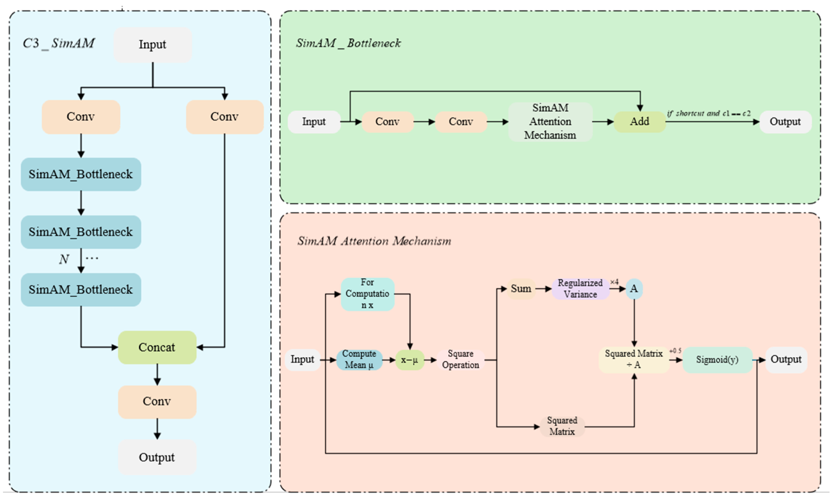
SimAM extracts the importance of neurons by constructing an energy function. Its core idea is based on the local self-similarity of images, generating attention weights by calculating the similarity between each pixel in the feature map and its neighboring pixels [27]. The SimAM calculation formula can be expressed as follows:

$$w_i = \frac{1}{k}{\sum }_{j\in N_i}s(f_{i },f_j )$$

(3)

where ${\mathit{w}}_{\mathit{i}}$ is the attention weight for pixel $\mathit{i}$, $\mathbf{k}$ is the normalization constant, ${\mathit{N}}_{\mathit{i}}$ is the set of neighboring pixels for pixel $i$, and $\mathit{s}({\mathit{f}}_{\mathit{i}},\mathit{}{\mathit{f}}_{\mathit{j}})$ is the similarity metric between pixel $\mathit{i}$ and pixel $\mathit{j}$, typically represented as the negative Euclidean distance: $\mathbf{s}({\mathbf{f}}_{\mathbf{i}},\mathbf{}{\mathbf{f}}_{\mathbf{j}})=-{\Vert {\mathbf{f}}_{\mathbf{i}}-{\mathbf{f}}_{\mathbf{j}}\Vert }_2^2$.

(3)

CBAM Attention Mechanism

It enhances the feature representation ability of convolutional neural networks by combining channel attention and spatial attention. The output of its channel attention module can be calculated using the following formula:

$$M_c (F)=\sigma (MLP(AvgPool(F))+MLP(MaxPool(F)))$$

(4)

where $\mathit{F}$ is the input feature map, $\mathit{A}\mathit{v}\mathit{g}\mathit{P}\mathit{o}\mathit{o}\mathit{l}$ and $\mathit{M}\mathit{a}\mathit{x}\mathit{P}\mathit{o}\mathit{o}\mathit{l}$ denote global average pooling and max pooling operations, respectively, $\mathbf{M}\mathbf{L}\mathbf{P}$ represents a multilayer perceptron, and $\mathsf{\sigma }$ denotes the Sigmoid activation function. The output of the spatial attention module is computed via the following formula:

$$M_s (F)=\sigma (f^{7\times 7}([AvgPool(F);MaxPool(F)]))$$

(5)

where f^7×7 denotes a convolutional operation of 7 × 7, used to learn spatial attention weights from concatenated average-pooled and max-pooled feature maps.

2.4. Improved Loss Function

During the training of the YOLOv5 network model, the loss calculation expression is as follows.

$$L_{CIoU}=1-CIoU=1-(IoU-\frac{d_0^2}{d_c^2}-\frac{v^2}{(1-IoU+v)})$$

(6)

$$v=\frac{4}{{\pi }^2}(arctan\frac{w^{gt}}{h^{gt}}-arctan\frac{w^p}{h^p}{)}^2$$

(7)

where ${\mathit{L}}_{\mathit{C}\mathit{I}\mathit{o}\mathit{U}}$ is the corresponding loss function, $\mathit{I}\mathit{o}\mathit{U}$ is the intersection-over-union ratio between anchor boxes and target boxes, ${\mathit{d}}_0$ is the distance between anchor boxes and target boxes, ${\mathit{d}}_{\mathit{c}}$ is the diagonal distance of target boxes, $\mathit{v}$ is the parameter used to judge the difference in aspect ratio between anchor boxes and target boxes, ${\mathit{w}}^{\mathit{g}\mathit{t}}$ and ${\mathit{h}}^{\mathit{g}\mathit{t}}$ are the width and height of target boxes, and ${\mathit{w}}^{\mathit{p}}$ and ${\mathit{h}}^{\mathit{p}}$ are the width and height of anchor boxes.

(1)

Alpha-IoU Loss Function

The Alpha-IoU loss function is an extension of the traditional IoU loss function. It introduces an adjustable parameter α to modulate the gradient of the loss function, thereby accelerating model training convergence. The principle of the Alpha-IoU loss function can be expressed as follows:

$$L_{\alpha -IoU} =1-Io{U}^{\alpha }$$

(8)

where $\mathit{I}\mathit{o}\mathit{U}$ is the intersection-over-union ratio between the predicted bounding box and the ground truth bounding box, and $\mathit{\alpha }$ is a parameter greater than zero that controls the gradient of the loss function. By adjusting the value of $\mathit{\alpha }$, the gradient of the loss function becomes larger when IoU is high, accelerating model convergence in high-IoU regions. This leads to performance improvements in practical applications.

(2)

EIoU Loss Function

The EIoU loss function calculates the loss by considering the overlap area, center point distance, aspect ratio, and width-to-height ratio between the predicted box and the ground truth box [28]. Its formula can be expressed as follows:

$$L_{EIoU} =1-IoU+\frac{{\rho }^2(b,b^{gt})}{c^2} + \frac{{\rho }^2(w,w^{gt})}{C_w^2} + \frac{{\rho }^2(h,h^{gt})}{C_h^2}$$

(9)

where $\mathit{I}\mathit{o}\mathit{U}$ is the intersection-over-union ratio between the predicted and ground truth boxes, $\mathit{\rho }(\mathit{b},{\mathit{b}}^{\mathit{g}\mathit{t}})$ denotes the Euclidean distance between the centers of the predicted and ground truth boxes, $\mathit{c}$ is the diagonal length of the minimum bounding region encompassing both boxes, $\mathit{w}$ and $\mathit{h}$ represent the width and height of the predicted and ground truth boxes, respectively, and ${\mathit{C}}_{\mathit{w}}$ and ${\mathit{C}}_{\mathit{h}}$ are the diagonal lengths of the bounding regions for width and height, respectively.

2.5. Improving the YOLOv5s Network Architecture

The YOLOv5 models are categorized from smallest to largest as YOLOv5n, YOLOv5s, YOLOv5m, and YOLOv5l. While the traditional YOLOv5s offers advantages such as lightweight architecture and fast detection speed, it suffers from insufficient feature expression focus and limited bounding box regression accuracy. Therefore, this paper introduces several improvements to the YOLOv5s model. These include integrating SimAM into the backbone network and replacing the CIoU loss function in YOLOv5 with the EIoU loss function. The overall network architecture is shown in Figure 3, and the SimAM submodule is shown in Figure 4. Since obstacle datasets typically contain objects of various shapes and sizes, this architecture helps the model better capture and recognize these objects, thereby optimizing the performance of YOLOv5s.

3. Experiments and Results

This chapter will conduct a comprehensive evaluation of the improved model’s performance through systematic experimental validation. It details the experimental setup, dataset partitioning, and metric selection to establish objective benchmarks. Through ablation studies, it quantifies the specific contributions of image preprocessing, attention mechanisms, and loss function optimization to model accuracy, validating the rationality of the improvement strategy. This demonstrates the model’s accuracy and robustness when applied to dynamic obstacle avoidance tasks for cranes in complex working environments.

3.1. Model Training

3.1.1. Image Acquisition

In the actual working scenarios of cranes, common obstacles include workers, construction materials, and other equipment. These obstacles vary in shape, size, and color, and may change dynamically during operation. To simulate these obstacles in a laboratory environment, appropriate alternative items need to be selected to ensure the feasibility and effectiveness of the experiment. By using alternative items, an experimental environment close to the actual working scenario can be constructed in the laboratory, thereby facilitating the verification and optimization of the obstacle detection model’s performance.

During the dataset construction process, to cover three main categories (materials, various obstacles, and workers), 320 images of cartons (materials), 300 images of roadblocks (Obstacle 1), 400 images of mineral water buckets (Obstacle 2), 300 images of water pails (Obstacle 3), and 300 photos of workshop workers (workers) were collected. The image capture device was set to a resolution of 1920 × 1080,with the capture location situated in the simulated crane operation area of the laboratory. All images were imported into Photoshop and resized to 640 × 640 pixels to meet the optimal size requirement for model training. Subsequently, the selected dataset was annotated using LabelImg (version 1.8.6). Finally, the dataset was split into a training set and a validation set at a ratio of 3:1.

3.1.2. Training Environment and Parameter Configuration

To clearly present the experimental conditions and ensure the reproducibility of the study, the specific configuration of the training environment is detailed in

Table 1. Training environment and parameter configuration.

Environmental Parameters	Configuration
Operating System	Windows 10
Central Processing Unit (CPU)	i7-14700KF
GPU	RTX 4060Ti (8GB)
Training Framework	PyTorch 1. 11. 0
Programming Language	Python 3. 8

.

In all experiments, the training parameters of different models were kept consistent, and the configuration of the training parameters are detailed in

Table 2. Parameter configuration.

Parameters	Values
Epoch	300
Batch Size	2
Image Size	640 × 640
Initial Learning Rate	0.01
Weight Decay Coefficient	0.0005
Learning Rate Momentum	0.937
Optimizer	SGD (Stochastic Gradient Descent)

.

3.2. Evaluation Metrics Commonly Used in Object Detection

(1)

Precision

Precision measures the reliability of the model’s detection results, representing the proportion of samples correctly classified as positive among all samples predicted as positive. The formula is as follows:

$$\mathrm{Precision}={\displaystyle \frac{TP}{TP+FN}}$$

(10)

(2)

Recall

Recall is defined as the proportion of true positives (TP) out of all actual positive samples (TP + FN), reflecting the model’s ability to identify positive samples. As the confidence threshold increases, the classifier’s predictions become stricter, potentially leading to reduced recall because more positive samples are incorrectly classified as negative. The formula is as follows:

$$\mathrm{Recall}={\displaystyle \frac{TP}{TP+FN}}$$

(11)

(3)

Average Precision (AP)

Precision and recall are a pair of mutually contradictory metrics that typically vary with changes in confidence thresholds [29]. To comprehensively evaluate a category’s precision performance across different recall levels, we plot a precision–recall curve. AP represents the area under this P–R curve, providing a single metric summarizing the model’s overall performance on a given category. A higher AP value indicates the model is both accurate and comprehensive for that category. Its calculation typically employs the interpolation method from the PASCAL VOC challenge: AP = ${\displaystyle {\sum }_{\mathrm{i}+1}^{\mathrm{n}}}(R_{\mathrm{i}+1}-R_{\mathrm{i}})\ast P_{\mathrm{interp}}(R_{\mathrm{i}+1})$, where $P_{\mathrm{interp}}(R_{\mathrm{i}+1})$ = max $\tilde{R}\tilde{R}\ge P(\tilde{R})$. This involves finding the maximum precision among all points where recall is no less than Ri + 1, and interpolating that value.

(4)

Mean Average Precision (mAP)

This is the most fundamental global evaluation metric in multi-class object detection. It calculates the average of AP across all classes. In this study, we primarily report mAP at an IoU threshold of 0.5, serving as a crucial indicator for assessing a model’s recognition capability under relaxed localization requirements.

(5)

mAP@0.5:0.95

To rigorously evaluate a model’s localization accuracy, we also adopt the COCO dataset evaluation standard by computing the average AP across multiple IoU thresholds (from 0.5 to 0.95, incremented by 0.05). This metric demands high overlap between predicted and ground truth bounding boxes, providing a more comprehensive reflection of the model’s overall localization performance.

(6)

Detection Speed

Detection speed refers to the pure inference time from inputting a single image to outputting obstacle detection results, measured in milliseconds, reflecting the model’s real-time capability.

(7)

F1 Score (F1–Confidence Curve)

The F1 score, as the harmonic mean of precision and recall, provides a comprehensive metric to evaluate the performance balance of a model across different decision thresholds [30].

3.3. Comparison of Training Performance Across Different Models

In crane obstacle avoidance environments, selecting an appropriate YOLOv5 model is crucial for achieving efficient and accurate object detection [31]. The YOLOv5 series offers multiple models varying in size and complexity, including YOLOv5n, YOLOv5s, YOLOv5m, and YOLOv5l. Each model exhibits distinct characteristics in detection speed and accuracy, making them suitable for different application scenarios. No pre-trained weights were utilized during training to ensure the model was specifically tailored for obstacle detection tasks in crane operating environments. By comparing the training results of these four models on the dataset, we can conduct an in-depth analysis of their differences in detection speed, accuracy, and resource consumption.

For safety systems in gantry cranes operating under constrained computational resources, balancing detection accuracy with real-time performance is critical. According to

Table 3. Training performance comparison of different models.

Model	Average Precision	Average Recall	F1 Score	mAP@0.5	Inference Speed	Training Time	Model Size
YOLOv5n	0.785	0.742	0.763	0.762	16	5.525 h	7.5
YOLOv5s	0.852	0.818	0.835	0.835	18	5.428 h	14.1
YOLOv5m	0.893	0.837	0.845	0.874	25	5.385 h	43.7
YOLOv5l	0.911	0.885	0.893	0.903	32	8.764 h	89.2

data, YOLOv5l achieves the highest mAP@0.5, but its detection speed is significantly lower than that of YOLOv5s. YOLOv5s achieves a balance between accuracy, recall, and real-time capability, while also requiring shorter training time than YOLOv5m. Therefore, YOLOv5s is selected as the baseline model for subsequent improvements.

3.4. Detection Results

3.4.1. Preprocessing Optimization Results and Analysis

To address issues such as fluctuating illumination, noise interference, and blurred obstacle edges in crane operation scenarios, this study designed a multi-stage preprocessing workflow incorporating Sobel sharpening, bilateral filtering, and Enlighten-GAN low-light enhancement. By training on low-brightness datasets, its effectiveness was validated through image quality evaluation metrics and model detection performance.

Based on the data in

Table 4. Preprocessing optimization results.

Preprocessing Steps	Precision	Recall	mAP@0.5	PSNR (dB)	SSIM
Original Low-Light	0.852	0.818	0.835	14.85	0.423
Enlighten-GAN	0.867	0.861	0.849	23.4	0.68
Bilateral Filter	0.873	0.825	0.852	26.1	0.75
Sobel Sharpening	0.858	0.832	0.846	25.8	0.73
Our	0.892	0.871	0.912	32.1	0.89

, the recognition performance and image quality for obstacles in complex dynamic environments involving cranes have been significantly improved following preprocessing optimization.

3.4.2. Comparison with Attention Mechanisms

We compared SimAM with two mainstream attention mechanisms, SE and CBAM. As shown in the model training results in Figure 5, SimAM demonstrates significant superiority over both SE and CBAM. SimAM infers 3D attention weights in feature maps by constructing an energy function. This approach enables SimAM to effectively enhance CNN performance without adding extra parameters, particularly outperforming other attention mechanisms in mean average precision (mAP_0.5:0.95).

3.4.3. Introducing Loss Function Comparison

The loss function is employed to optimize bounding box regression accuracy. Figure 6 illustrates the recognition results for the same image before and after adding the Alpha-IoU and EIoU loss functions. Comparison reveals that incorporating the Alpha-IoU loss function improves the model’s recognition accuracy for Obstacle 2 in low-brightness scenes from 0.76 to 0.86, while the model’s accuracy for Obstacle 2 in low-brightness scenes improved from 0.76 to 0.89 after incorporating the EIoU loss function. Comparative analysis of both loss functions, combined with detection performance on the test set, reveals that the EIoU loss function delivers particularly significant improvements.

3.4.4. Loss Function

The improved YOLOv5s output employs EIoU_Loss as the loss function for bounding boxes. A lower value indicates greater prediction accuracy. Obj_Loss represents the average objective loss, where a lower value indicates more accurate object detection. Cls_Loss denotes the average classification loss, with a smaller value signifying more precise classification. The results are shown in Figure 7. Training results indicate convergence after 250 iterations, ultimately stabilizing at a low level. The training loss curve exhibits no significant fluctuations, and the validation loss shows no divergence, demonstrating excellent stability in model training.

3.4.5. Recognition Accuracy Analysis

The recognition performance of the three models—YOLOv5s, YOLOv5s_SimAM, and the improved YOLOv5s—is shown in Figure 8. As illustrated, introducing the EIoU loss function to refine the L_LOSS calculation method and the SimAM attention mechanism resulted in improvements across all metrics for the enhanced model. Notably, the detection performance for barriers showed a more pronounced increase due to the strengthened weighting for small object detection.

The average recognition accuracy results for all images of people and four simple obstacles are shown in

Table 5. Recognition accuracy rates for different types of obstacles.

Model	Person	Carton	Roadblock	Mineral Water Barrel	Bucket
Yolov5s	0.87	0.88	0.90	0.89	0.92
YOLOv5s + SimAM	0.89	0.90	0.91	0.91	0.93
YOLOv5s + EIoU	0.91	0.93	0.94	0.93	0.95
YOLOv5s + SimAM + EIoU	0.93	0.95	0. 96	0.95	0.95

. As indicated in Table 5, both SimAM and EIoU contribute to improving recognition accuracy. When SimAM and EIoU are introduced simultaneously, the average recognition accuracy increases by 6% compared to the traditional Yolov5s model.

3.4.6. Ablation Study

To validate the effectiveness of each improvement module, we conducted ablation experiments on the same dataset after preprocessing each model. The results are shown in

Table 6. Comparison of ablation experiment results.

Model	Precision	Recall	mAP@0.5	Params	GFLOPs	Model Size
Yolov5s	0.892	0.871	0.912	7.3	17.3	14.1
YOLOv5s + SimAM	0.908	0.915	0.934	7.3	17.8	14.1
YOLOv5s + EIoU	0.932	0.884	0.939	7.3	17.3	14.1
YOLOv5s + SimAM + EIoU	0.946	0.938	0.952	7.3	17.8	14.1

.

As shown in Table 6, incorporating the SimAM attention mechanism and EIoU loss function improves obstacle regression accuracy and significantly enhances the model’s detection precision across various target categories. The performance markedly outperforms the original YOLOv5s model, with detection speeds consistently below 30 ms including preprocessing time, meeting real-time industrial obstacle detection requirements.

3.4.7. Experimental Comparison

To validate the obstacle recognition performance of this study under real-world conditions, obstacle detection tests were conducted using indoor gantry cranes in specific operational scenarios. Three different-sized reducers (large, medium, and small) were tested at varying distances and visibility levels. The recognition results are shown in Figure 9, Figure 10 and Figure 11. The corresponding recognition accuracy is detailed in

Table 7. Real-world obstacle detection performance of the reducer.

Operating Conditions	Distance (Large-Scale Reducer)			Size (Short Distance)			Visibility (Large-Scale Reducer)
	Short	Medium	Long	Small	Medium	Large	Low	Medium	High
Precision	0.96	0.92	0.84	0.86	0.89	0.92	0.83	0.88	0.92

. As shown in Table 7, recognition accuracy gradually decreases as reducer size decreases, distance increases, and visibility decreases, with a total reduction of 9%. However, the improved model achieves detection speeds within 30 milliseconds. Therefore, obstacle recognition should be performed at the closest possible distance. Additionally, the crane obstacle recognition system should incorporate lighting devices to accommodate recognition requirements in low-visibility operational environments.

4. Comparative Experiment

To further evaluate the overall recognition performance of the improved model for reducer obstacles, the comparative analysis of recognition capabilities was conducted between the improved model and mainstream YOLO models, including comparison of different attention mechanisms and loss-of-function conditions in the improved model.

4.1. Comparison Results of Mainstream YOLO Models

Table 8. Comparative experimental results of different YOLO models.

Model	Precision	Recall	mAP@0.5	Params (M)	GFLOPs	Model Size (MB)
YOLOv5s	0.868	0.816	0.855	7.3	17.3	14.1
YOLOv8s	0.872	0.756	0.851	11.1	28.6	22.5
YOLOv10s	0.855	0.851	0.864	8.2	24.6	16.6
YOLOv11s	0.881	0.811	0.871	9.4	21.3	19.6
Our	0.891	0.845	0.884	7.3	17.8	14.1

presents the overall recognition results for reducer obstacles under varying sizes, distances, and visibility conditions, comparing the improved model with existing mainstream YOLO models. Table 8 indicates that the improved model outperforms mainstream YOLO models in overall accuracy, mAP@0.5, parameter count, computational cost, and model size, while recall was only 0.7% lower than YOLOv10s, but the computational complexity was reduced by 27.6%. Consequently, the improved model achieves overall enhanced performance in reducer obstacles detection while requiring fewer computational resources.

4.2. Comparison Results of Different Attention Mechanisms

The comparison results of simple simulated obstacles obtained with the improved model in this paper demonstrate that the SimAM attention mechanism exhibits remarkable superiority. To further verify the performance of the SimAM attention mechanism in reducer obstacles recognition, the SE, ECA, and CBAM attention mechanisms were separately integrated into the improved model under the premise of keeping all other conditions unchanged, and the corresponding experimental comparison results were presented in

Table 9. Comparative experimental results of different attention mechanisms.

Attention Mechanism	Precision	Recall	mAP@0.5
SE	0.872	0.836	0.876
ECA	0.878	0.832	0.874
CBAM	0.886	0.829	0.873
SimAM (Our)	0.891	0.845	0.884

. Table 9 shows the SimAM attention mechanism integrated into the improved model can increase nearly 1% in mAP@0.5 compared with the SE, ECA, and CBAM attention mechanisms.

4.3. Comparison Results of Different Loss Functions

Under other constant conditions, the experimental comparison results of reducer obstacles recognition used the improved YOLO model with different loss functions, and are shown in

Table 10. Comparative experimental results of different loss functions.

Loss Function	Precision	Recall	mAP@0.5
Alpha-IoU	0.875	0.828	0.869
SIoU	0.888	0.838	0.878
WIoU	0.885	0.848	0.887
EIoU (Our)	0.891	0.845	0.884

. The results show that the overall performance of reducer obstacle recognition was basically consistent when the EIoU and WIoU loss functions were adopted, and EIoU achieves a higher precision while WIoU performs better in terms of recall and mAP@0.5. EIoU exhibits superior performance in precision, recall, and mAP@0.5 compared with Alpha-IoU and SIoU, while the mAP@0.5 increases 1.7% and 0.7%, respectively. The experimental results indicate that both EIoU and WIoU have better recognition performance for reducer obstacle recognition in the crane operation scenario.

5. Conclusions

This paper proposes an improved YOLOv5s model capable of detecting people and obstacles in complex gantry crane operation scenarios. Through experiments involving human, simple obstacle, and reducer detection, the model demonstrates enhanced recognition performance. The conclusions drawn from the research are presented as follows.

(1)

Preprocessing techniques such as image sharpening, adaptive denoising, and low-light image enhancement significantly improve image quality and recognition accuracy;

(2)

The improved model achieves an average recognition accuracy exceeding 0.93 for people and simple obstacles, representing a 5.4% improvement over traditional methods with preprocessing detection speed under 30 ms;

(3)

The size, distance, and visibility of reducer obstacles significantly impact recognition accuracy; short-distance obstacle detection should be prioritized to enhance accuracy with the high-speed recognition advantage of the improved model.

(4)

The improved YOLOv5s model demonstrates superior recognition performance compared to existing mainstream YOLO models while requiring fewer computational resources; the SimAM and EIoU used in the improved YOLOv5s model show better recognition accuracy.

Future work will involve comparative validation and analysis of obstacle recognition performance using new YOLO versions under adverse outdoor conditions such as rain, snow, and dense fog. Concurrently, we will deepen the optimization of attention mechanisms and loss functions to further unlock the model’s performance potential and adaptability to challenging environments.