Multibody for Everybody (M4E): A Symbolic Dynamics Modeling Tool with Applications in Simulation, Control, and Optimization

Abstract

Developing the analytical model of a multibody system is often the initial step in control and optimization. The analytical model (equations of motion) describes a system’s time evolution under specified forcing conditions. Although developing these equations is easy for simple systems, this process becomes more complex for systems composed of multiple bodies. Deriving equations of motion for complex multibody systems requires specialized expertise in multibody dynamics, is time-consuming, and is susceptible to error. To address this issue, this paper presents an open-source, easy-to-use, systematic framework to derive symbolic equations of motion in both Python and MATLAB using the joint coordinate formulation. This formulation results in a set of ordinary differential equations that use the minimum set of coordinates needed to model a system. The symbolic representation provides better insight into the influence of design parameters on system performance, facilitates sensitivity analysis and parameter studies, and supports direct implementation of control and optimization routines. The tool enables numerical simulation for specified parameter sets, is modular for straightforward integration with other tools and libraries, and allows incorporation of hydrodynamics, mooring, and other external forces. The result is a reproducible, extensible pipeline for modeling, simulation, and design of complex multibody systems. The proposed tool is versatile and can be applied to domains such as robotics, control, and design. In addition, we integrated external libraries that provide capabilities for modeling offshore systems such as underwater robots and marine energy converters.

1. Introduction

Deriving analytical equations of motion (EOM) is often considered the first step for control and optimization of a given system. Although modeling tools such as Ansys, Simscape, OpenFOAM, and OrcaFlex can be used to simulate complex systems, they do not provide the underlying EOM. While simple systems can be modeled by hand, manual derivation of the EOM for complex multibody systems can quickly become complicated, tedious, and error-prone [1]. Developing such models requires specialized expertise in multibody dynamics, yet accurate EOM are frequently needed by users who are not dynamics specialists. For example, engineers and researchers working in areas such as design optimization, robotics, biomechanics, or physics-informed machine learning often require the EOM without having specialized expertise in multibody dynamics. To bridge this gap, we present an open-source and user-friendly pipeline that automates the derivation of symbolic EOM using an efficient dynamics modeling framework. The symbolic representation enables a deeper mathematical analysis of the system, allowing parametric exploration of its behavior through examination of the coefficients in the differential equations.

1.1. An Overview of Multibody Dynamics Modeling Approaches

Two common approaches are used for modeling multibody systems. The first involves writing the Newton–Euler EOM for each body (as a set of differential equations) and applying the kinematic constraints imposed by joints as a set of algebraic equations. This results in a large system of differential–algebraic equations (DAEs) that use redundant coordinates (also known as absolute coordinates) to model the system [2,3].

The second approach employs a coordinate-reduction method that uses a smaller set of variables to represent the system [3,4]. This formulation can produce a reduced set of ordinary differential equations (ODEs), the size of which equals the number of degrees of freedom of the system, making it more efficient for control design, optimization, and design-space exploration. Notable examples of this formulation include Kane’s method [5] and the joint coordinate method [6]. The joint coordinate method offers an intuitive and systematic framework for modeling complex multibody systems. Because of these benefits, we use this formulation to generate the EOM [2,3,4,7].

1.2. An Overview of the Existing Multibody Dynamics Tools and Modeling Gaps

Many existing open-source and proprietary modeling tools rely on the Newton–Euler formulation to simulate system dynamics because of its relative simplicity [8,9,10]. However, as discussed in Section 1.1, a joint coordinate formulation is more desirable for control and optimization applications. To the best of our knowledge, PyDy is currently the only open-source modeling tool that provides analytical EOM using reduced coordinates [1]. Nevertheless, effective use of PyDy still requires expertise in multibody dynamics, particularly in Kane’s method. As a result, the framework presented in this work is the first free, open-source tool that enables users without a background in multibody dynamics to automatically derive, visualize, and analyze EOM. This platform is available in both Python (https://github.com/Project-SEA-Stack/Python_Multibody_for_Everybody accessed on 15 January 2026) and MATLAB (https://github.com/Project-SEA-Stack/MATLAB_Multibody_for_Everybody accessed on 15 January 2026), although this work focuses on the Python version for brevity.

With our tool, users can simply specify the location of the center of gravity (CG) for each body, the location of the joints, and the external forces, and the tool handles the development of the EOM. Crucially, the interface is designed so that engineers with little or no multibody background can use it; the pipeline handles all the complex math behind the scenes. Our tool also provides built-in animation and plotting of the simulated motion, so users can immediately verify and visualize their models. In addition, the symbolic output makes explicit how design parameters impact the dynamics equation, which facilitates sensitivity analysis and design optimization. Because the model is available in symbolic form, it can also be incorporated into physics-informed machine learning workflows, enabling data-driven optimization or estimation that respects the true system dynamics.

1.3. Contributions

This work makes the following contributions:

1.

An open-source, user-friendly multibody dynamics pipeline (in Python and MATLAB) that automates derivation, simulation, and analysis of a system’s EOM (using the joint coordinate formulation) in 2D (the 3D work is under progress).

2.

A low-barrier interface and built-in visualization (animation and plotting) capability that lets non-experts model a system by specifying minimal inputs (body centers of gravity, joint locations, and external forces).

3.

Full symbolic parameterization of the model (e.g., masses, inertias, joint locations, spring attachment locations, hydrodynamic coefficients), enabling algebraic sensitivity analysis, symbolic design-space definitions, symbolic evaluation of constraint forces, and rapid substitution for numerical studies.

4.

A modular external force manager designed for seamless integration with third-party tools as well as an extendable template that simplifies incorporation of external forces computed from other tools.

5.

Existing coupling with marine energy tools MoorDyn and Capytaine [11,12].

6.

Providing the equations of motion in a form suitable for linearization (applicable to controller synthesis, frequency-domain modeling, and stability analysis).

7.

Comprehensive documentation spanning more than 100 pages, detailing the tool’s features and providing numerous solved examples.

1.4. Paper Organization

The remainder of this paper is organized as follows: Section 2 discusses the mathematical framework used for generating EOM. Section 3 presents the code structure and architecture. Section 4 includes several examples used to verify our code. Section 5 provides various examples and tutorials illustrating how different systems can be modeled. Section 6 discusses how the generated EOM can be used for linearization, optimization, and control. Section 7 describes limitations and future work, and Section 8 provides the conclusion. Section 9 describes the GitHub repository, installation instructions, example datasets, documentation, and tests.

2. Theory

Dynamics modeling of multibody systems has been heavily studied. For this reason, this work only briefly discusses the mathematical framework implemented to generate the dynamics model (the reader may refer to [13,14] for more detail). As discussed in Section 1.1, modeling multibody systems with the Newton–Euler formulation results in DAEs, whereas methods such as joint coordinate lead to ODEs. We start by developing the EOM using the Newton–Euler approach, followed by implementing a systematic framework to convert these equations into ODEs using the joint coordinate method.

2.1. Notations

Throughout this paper, boldface letters indicate matrices and vectors, whereas light-face letters denote scalar quantities. A global frame $X-Z$ is located at point O as shown in Section 3.1. The position and orientation of this frame remain stationary. A body-fixed frame ${\xi }_i-{\eta }_i$ is placed at the CG of each body. This frame translates and rotates with the body that is attached to it. Throughout this paper, vectors are represented in the global frame, unless explicitly stated otherwise. In M4E, the ${\xi }_i-{\eta }_i$ frame is initially parallel to the global frame. When initiating a simulation, users can provide an arbitrary angle between these two frames. This defines the angle that the positive Z axis makes with the ${\eta }_i$ axis, measured clockwise from Z towards ${\eta }_i$.

2.2. Modeling Constrained Multibody Systems Using the Newton–Euler Method

The EOM for a constrained multibody system composed of n bodies can be written as

$$\begin{array}{c}\mathcal{M}\dot{\mathit{v}}=\mathit{g}+{\mathit{g}}_g+{\mathit{g}}_c,\hfill \end{array}$$

(1)

where

$$\begin{array}{cc}\hfill & \mathcal{M}=\left[\begin{array}{ccc}{\mathcal{M}}_1& & \\ {\mathcal{M}}_2& & \\ & \ddots & \\ & & {\mathcal{M}}_n\end{array}\right],\dot{\mathit{v}}=\left[\begin{array}{c}{\dot{\mathit{v}}}_1\\ {\dot{\mathit{v}}}_2\\ ⋮\\ {\dot{\mathit{v}}}_n\end{array}\right],{\mathit{g}}_g=\left[\begin{array}{c}{\mathit{g}}_{g_1}\\ {\mathit{g}}_{g_2}\\ ⋮\\ {\mathit{g}}_{g_n}\end{array}\right],\mathit{g}=\left[\begin{array}{c}{\mathit{g}}_1\\ {\mathit{g}}_2\\ ⋮\\ {\mathit{g}}_n\end{array}\right]\hfill \\ \hfill & {\mathcal{M}}_i=\left[\begin{array}{cc}{m}_i{\mathit{I}}_2& 0\\ 0& J_i\end{array}\right],{\dot{\mathit{v}}}_i=\left[\begin{array}{c}{\ddot{\mathit{r}}}_{P_i}\\ {\dot{\omega }}_i\end{array}\right],{\mathit{g}}_{g_i}=\left[\begin{array}{c}0\\ -m_{i}g\\ 0\end{array}\right],{\mathit{g}}_c={\mathit{D}}^T\mathit{\lambda }.\hfill \end{array}$$

(2)

Here, ${\mathit{I}}_2$ is a $2\times 2$ identity matrix. The mass of body i is $m_i$, and the moment of inertia about CG is $J_i$. The angular velocity in the global reference frame is ${\omega }_i$, and ${\ddot{\mathit{r}}}_{P_i}$ denotes the translational acceleration of the body i’s CG. The velocity vector ${\mathit{v}}_i\in {\mathbb{R}}^{3\times 1}$ combines the linear velocity of CG and the angular velocity; its time derivative is the acceleration vector ${\dot{\mathit{v}}}_i$. The $3\times 1$ array of force/moment ${\mathit{g}}_i$ gathers external forces and moments calculated about the CG of each body (e.g., from springs, dampers, drag, gravity, or propellers). For simplicity, the array of force/moment is referred to as “array of forces” throughout this paper. Additionally, ${\mathit{g}}_{g_i}$ presents the array of gravitational forces. The term ${\mathit{g}}_c={\mathit{D}}^T\mathit{\lambda }$ shows the array of unknown constraint forces, where $\mathit{D}$ is the Jacobian matrix of the kinematic constraints and $\mathit{\lambda }$ is the array of unknown Lagrange multipliers [13].

The ODE system shown in Equation (1) contains more unknowns ($\mathit{\lambda }$ and $\dot{\mathit{v}}$) than equations and thus cannot be solved. To overcome this issue, it is possible to append the kinematic constraints to this equation and solve for the unknowns (the reader can refer to Chapter 2 of [13] for more detail).

2.3. Modeling Constrained Multibody Systems Using the Joint Coordinate Method

This method projects the Newton–Euler equations discussed in Equation (1) onto the joint coordinate space. To achieve this for a system with m degrees of freedom (DOF), we first select a set of m independent velocities, $\dot{\mathit{q}}$, that can describe the system. Then, using the kinematic constraint, we can find a velocity transformation matrix $\mathit{B}$ that maps $\dot{\mathit{q}}$ to $\mathit{v}$,

$$\mathit{v}=\mathit{B}\dot{\mathit{q}}.$$

(3)

Then, we can find the array of acceleration by taking the time derivative of Equation (3):

$$\dot{\mathit{v}}=\mathit{B}\ddot{\mathit{q}}+\dot{\mathit{B}}\dot{\mathit{q}}.$$

(4)

Finally, by substituting the value of $\dot{\mathit{v}}$ from Equation (4) into Equation (1) and left-multiplying Equation (1) by ${\mathit{B}}^T$, we can find the EOM in joint coordinate:

$${\mathit{B}}^T\mathit{M}\mathit{B}\ddot{\mathit{q}}={\mathit{B}}^T(\mathit{g}+{\mathit{g}}_g)-{\mathit{B}}^T\mathit{M}\dot{\mathit{B}}\dot{\mathit{q}}.$$

(5)

It must be mentioned that the array of constrained forces ${\mathit{g}}_c={\mathit{D}}^T\mathit{\lambda }$ is eliminated, as $\mathit{B}$ lies in the null space of $\mathit{D}$ [3,13]. We rely on this formulation to model multibody systems throughout this paper.

2.4. Systematic Assembly of the B Matrix

The primary objective of M4E is the construction of the velocity transformation matrix $\mathit{B}$. The assembly of the equations of motion for a general multibody system is nontrivial, and a complete derivation is beyond the scope of this work; detailed treatments can be found in [15,16,17]. Here, we outline the algorithmic steps required to assemble the $\mathit{B}$ matrix, assuming that the system topology and joint definitions are already available.

In M4E, a multibody system is represented using a graph-based formulation. The resulting graph is organized into branches that describe how bodies are connected to one another. Each branch originates at a root body that is directly connected to the ground body and extends outward through successive child bodies. Additionally, each joint type is associated with a prescribed set of joint coordinates (degrees of freedom). For every joint connection (joints defined in M4E include information about the parent body, child body, and joint type), these joint coordinates are assigned to the corresponding child body. For each branch, bodies are then numbered in increasing order according to their topological distance from the ground body, with the body closest to the ground assigned the lowest index. In systems with multiple branches, the specific numbering between branches is arbitrary, provided that the previous ordering rule is respected.

Once the body indices are defined, the system is re-ordered into an arithmetic sequence $(1,2,3,\dots )$ based on the assigned body numbers. The multibody topology is then represented as a directed graph, constructed using the networkx library in Python or the digraph class in MATLAB. This graph representation enables the automatic identification of all kinematic branches and the bodies belonging to each branch, which is a prerequisite for assembling the $\mathit{B}$ matrix. This procedure is summarized in Algorithm 1.

This workflow creates the B matrix as an assembly of predefined submatrices. These submatrices are stored in a lookup table, where for each type of joint, there is a matrix for the parent body ${\mathit{B}}_{ii}$ and the children ${\mathit{B}}_{ji}$.

Notation: $\mathrm{Rows}\left(j\right)=[3j-2,3j-1,3j]$ selects the three rows associated with $(v_x,v_z,\omega )$ of body j. $\mathrm{Cols}\left(j\right)$ selects the column(s) associated with body j (one column for R/P, and three columns for F).

Algorithm 1 Branch-based column-first assembly of the velocity transformation matrix $\mathbf{B}\left(q\right)$ in 2D.

Require: $\mathcal{P}={\left\{{\pi }_{\ell }\right\}}_{\ell =1}^{N_{\mathrm{br}}}$ is the set of all root-to-leaf paths of the directed multibody tree (for example, ${\pi }_2=[4,5,\dots ,8]$); each branch is ordered from ground outward; joint types $\mathtt{Type}\left(j\right)\in \{R,P,F\}$; generalized coordinates q; geometry vectors parentCG2joint (j) and joint2childCG (j) for each body j (see Section 3.1); lookup-table submatrices routines ${\mathit{B}}_{jj}\left(·\right)$ and ${\mathit{B}}_{kj}\left(·\right)$. 1: Initialize $\mathbf{B}\leftarrow {\mathbf{0}}_{3N_b\times N_q}$          ▷$N_b\triangleq$ number of bodies, $N_q\triangleq$ system’s DOF 2: Initialize boolean tracking matrix ${\mathbf{B}}_{\mathrm{track}}\leftarrow {\mathbf{0}}_{N_b\times N_b}$  ▷${\mathbf{B}}_{\mathrm{track}}(k,j)=1$ once block ${\mathbf{B}}_{kj}$ is written 3: for each branch ${\pi }_l\in \mathcal{P}$ do 4:     ${\theta }_{\mathrm{parent}}\leftarrow 0$ 5:     for each body index j in ${\pi }_l$ (in order) do 6:          $\mathbf{p}\mathbf{2}\mathbf{j}\leftarrow \mathtt{parentCG}\mathtt{2}\mathtt{joint}\left(j\right)$;    $\mathbf{j}\mathbf{2}\mathbf{c}\leftarrow \mathtt{joint}\mathtt{2}\mathtt{childCG}\left(j\right)$▷ defining symbolic expressions $\mathbf{p}\mathbf{2}\mathbf{j}\left(\mathit{q}\right),\mathbf{j}\mathbf{2}\mathbf{c}\left(\mathit{q}\right)$ 7:          if $\mathtt{Type}\left(j\right)=P$ then        ▷ if prismatic, get angular position of parent 8:             ${\theta }_j^{\mathrm{abs}}\leftarrow {\theta }_{\mathrm{parent}}$ 9:          else 10:            ${\theta }_j^{\mathrm{abs}}\leftarrow {\theta }_j$ 11:         end if 12:         ${\theta }_{\mathrm{parent}}\leftarrow {\theta }_j^{\mathrm{abs}}$ 13:         if ${\mathbf{B}}_{\mathrm{track}}(j,j)=0$ then 14:            $\mathbf{B}(\mathrm{Rows}\left(j\right),\mathrm{Cols}\left(j\right))\leftarrow {\mathbf{B}}_{jj}\left({\theta }_j^{\mathrm{abs}},\mathbf{p}\mathbf{2}\mathbf{j},\mathbf{j}\mathbf{2}\mathbf{c}\right)$ 15:            ${\mathbf{B}}_{\mathrm{track}}(j,j)\leftarrow 1$ 16:         end if 17:         for each body index k (children) appearing after j in the same branch ${\pi }_{\ell }$ do 18:            if ${\mathbf{B}}_{\mathrm{track}}(k,j)=0$ then 19:                $\mathbf{B}(\mathrm{Rows}\left(k\right),\mathrm{Cols}\left(j\right))\leftarrow {\mathbf{B}}_{kj}\left({\theta }_j^{\mathrm{abs}},\mathbf{p}\mathbf{2}\mathbf{j},\mathbf{j}\mathbf{2}\mathbf{c}\right)$ 20:                ${\mathbf{B}}_{\mathrm{track}}(k,j)\leftarrow 1$ 21:            end if 22:         end for 23:     end for 24: end for 25: return  $\mathbf{B}$

3. Overview of M4E

The goal of our tools is to generate the EOM in the form described in Equation (5). To achieve this, M4E needs to automatically calculate the DOF of the system, select the corresponding joint coordinates, calculate $\mathit{B}$ and $\dot{\mathit{B}}$, and calculate the array of applied forces $\mathit{g}$. This is achieved via the following steps:

1.

The user provides an input file that describes the kinematic joints used in the system and how they connect the corresponding bodies. The input file also defines the springs, dampers, and external forces applied to the system.

2.

The source code handles the construction of the EOM and their integration:

(a)

The multibody_core module constructs the kinematics of the system, calculates the force and moments (i.e., from springs or dampers), and generates the EOM discussed in Equation (5).

(b)

The ext_force_manager module introduces any other external forces to the system (i.e., forces that are computed separately from a different tool).

(c)

The checks, tables, plots, and validation modules are auxiliary tools to help the user define and visualize their system correctly.

3.

The output of the code (i.e., EOM, animations, plots) is provided to the user.

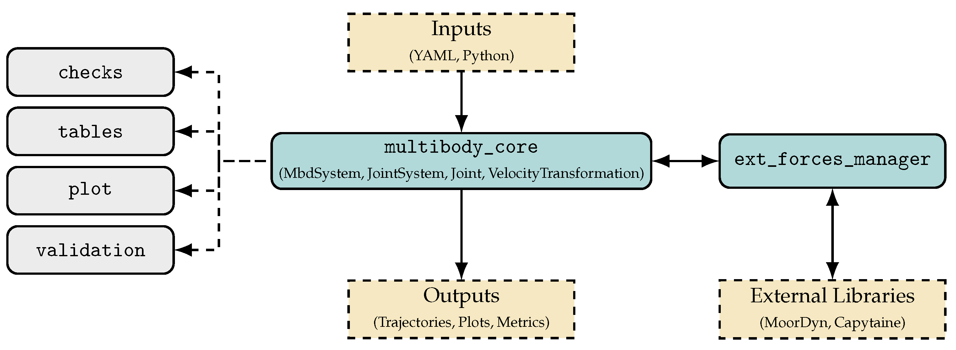
• A graphical explanation of these three steps is provided in Figure 1, and a detailed discussion of each step is provided below.

Figure 1. Compact high-level architecture of the framework. Core functionality is provided by MultibodyCore. External force models couple through ExtForcesManager, and auxiliary modules (Checks, Tables, Plotting, Validation) support verification, visualization, and reproducibility.

Figure 1. Compact high-level architecture of the framework. Core functionality is provided by MultibodyCore. External force models couple through ExtForcesManager, and auxiliary modules (Checks, Tables, Plotting, Validation) support verification, visualization, and reproducibility.

3.1. Inputs

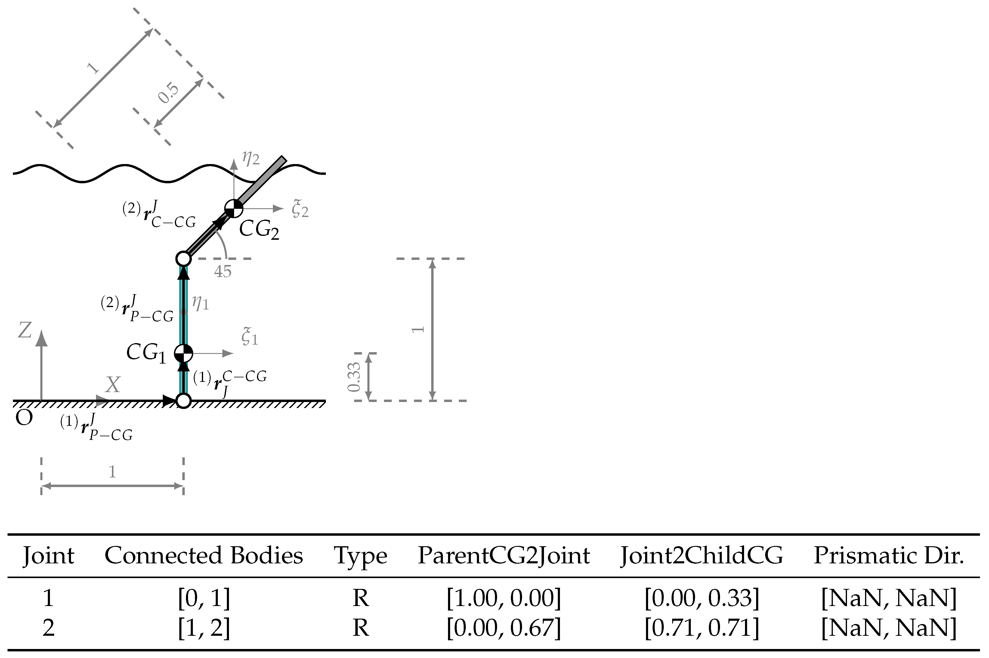
The input file could be either a Python file or a YAML file. For this work, we focus on the Python file; users can read the documentation on the YAML input if desired. Figure 2 outlines the variables the user must specify to define an example. A detailed explanation of how to define and format examples appears in Section 5. Each row of this table corresponds to a kinematic joint. The second column shows the parent body and child of joint j. The third column shows the joint type (the parent of the first body must be zero/ground). The available joints are floating joints (or 3-DOF joints), prismatic joints, and revolute joints.

For each joint, two vectors in the global frame (columns four and five) must be defined: ParentCG2joint and Joint2Childcg, respectively. Column four connects the parent center of gravity to the joint, while column five connects the joint to its child CG. The last column, Prismatic Dir., is only applicable to prismatic joints and defines the vector of the sliding direction. Running an input file in M4E, with the above definitions, leads to the schematics shown in Figure 2, where vector ${}^{\left(1\right)}\mathit{r}_{P-CG}^J$ shows the ParentCG2Joint vector of the first joint and ${}^{\left(1\right)}\mathit{r}_J^{C-CG}$ shows the Joint2ChildCG2 vector of the first joint.

3.2. Source Code

The source code is composed of six modules: multibody_core, ext_force_manager, checks, tables, plot, and validation (as shown in Figure 1). An overview of each module is provided below.

3.2.1. The multibody_core Module

The multibody_core module is implemented on top of SymPy to leverage symbolic capabilities that are valuable for design exploration, gradient computation, and control-oriented workflows. This module pursues three objectives: (i) building the symbolic EOM, (ii) writing the symbolic EOM in terms of executable functions, and (iii) managing the integration of EOM over time. These three goals are achieved within MbdSystem. The first two are tackled during the class initialization, but the last one is completed using a separate method.

The MbdSystem class constructs a connectivity graph showing hierarchical relationships between bodies and joints, where nodes represent bodies and are connected by edges (joints). In addition, the class stores attributes derived from joint definitions (see JointSystem and Joint for further details) together with dictionaries for points and forces assemble the symbolic EOM [16], generate executable functions [18], and manage the integration loop. The multibody system initialization and integration are handled by the following methods:

• __post_init__: assembles the symbolic EOM, compiles executable evaluators for efficient runtime, and verifies initial conditions
• integrate: performs numerical time integration.

Within __post_init__, the multibody connectivity graph and EOM come from the collection of Joint instances managed by JointSystem. The JointSystem class parses the information of all the joints, creates the symbolic variable associated with each DOF, and displays the bodies’ information in a table. It offers methods such as:

• from_data: constructs a joint system from lists (all of equal length), ordering bodies by child index;
• add_joint: instantiates a Joint per input record;
• display_table: presents system information in tabular form;
• coordinate_finder: creates symbolic variables (position, velocity, acceleration) for each DOF given the joint type (revolute, prismatic, floating).

• The Joint class stores the parent/child connectivity, joint type, and prismatic directions for each joint. Each Joint instance contains:

• parent: index of the parent body (0 denotes ground);
• child: index of the child body;
• joint_type: R/P/F for revolute, prismatic, or floating;
• parent_cg_to_joint: vector from the parent CG to the joint (global frame);
• joint_to_child_cg: vector from the joint to the child CG (global frame);
• prismatic_direction: unit vector, in the global frame, indicating the sliding direction for prismatic joints; NaN otherwise.

After building the JointSystem, the framework establishes the mapping between the global and joint velocities by forming the velocity transformation matrices B and $\dot{B}$ through VelocityTransformation [16]. The VelocityTransformation class maps joint velocities to global velocities using the $\mathit{B}$ matrix Equation (3), computes $\dot{\mathit{B}}$, and expresses the bodies’ CG and joint positions in terms of joint coordinates. This step detects grounded branches and recursively constructs connectivity via methods such as compute_grounded and compute_non_grounded.

Afterward, external loads are assembled by points_force_finder. This method identifies numeric or symbolic forces, registers the application points, and assembles them into a force vector ($\mathit{g}$ and ${\mathit{g}}_{nl}$ of Equation (5)). M4E supports six built-in force types:

• PointsBD: point forces not applied at the center of gravity;
• CG: point forces acting at the center of gravity;
• TensionSpring: linear/nonlinear tension spring between two points;
• TensionDamper: linear/nonlinear damper between two points;
• TorsionSpring: linear/nonlinear torsional spring between two joints;
• TorsionDamper: linear/nonlinear torsional damper between two joints.

• The next step of the initialization is the energy computation. This occurs within the systems_energy method. This method computes the system energy (kinetic plus potential), including linear/torsional springs. Lastly, MbdSystem assembles the EOM. The overall workflow is summarized in Algorithm 2.

Algorithm 2 System initialization and EOM symbolic assembly.

Require: Lists: parent, child, joint_type (R/P/F), parent_cg_to_joint, joint_to_child_cg, prismatic_direction; dictionaries: Initial_Points, Forces Ensure: Compiled MbdSystem with symbolic EOM, executable (lambdified) evaluators, B and $\dot{B}$ through the steps: 1: Conduct checks (optional) to validate list lengths, indices, prismatic normalization, and ground connectivity. 2: Create JointSystem ← JointSystem.from_data(parent, child, joint_type,                           parent_cg_to_joint, joint_to_child_cg, prismatic_direction). 3: For each Joint instance do JointSystem.add_joint → create a Joint with                           parent, child, joint_type, prismatic direction. 4: Assign symbolic DOFs via JointSystem.coordinate_finder(). 5: Build B, $\dot{B}$ via VelocityTransformation. 6: Populate a points dictionary and construct force dictionary for all supported types (PointsBD, CG, …) from points_force_finder. 7: Compute the analytical energy expression for the multibody system from systems_energy. 8: Assemble symbolic EOM (Equation (5)), in joint coordinate within MBDSystem                         $LHS={\mathit{B}}^{\top }\mathit{M}\mathit{B},RHS={\mathit{B}}^{\top }(\mathit{g}+{\mathit{g}}_g)-{\mathit{B}}^{\top }\mathit{M}\dot{\mathit{B}}\dot{\theta }$. 9: Compile EOM numeric evaluators via MbdSystem._compile_numeric. 10: Verify initial conditions through MbdSystem._ic_check. 11: Return compiled MbdSystem.

3.2.2. The ext_forces_manager Module

M4E is designed to be extended to a wide range of scientific and engineering domains beyond multibody dynamics. For that purpose, it separates multibody_core supported loads from domain-specific loads that are computed by other tools, thus avoiding changing the code structure every time new capabilities are added. The ExternalForcesManager class handles the communication of domain-specific loads from external providers and M4E. Each external provider implements a minimal interface following ExternalForcesManager guidelines and returns applied forces $\mathit{g}$. At runtime, the manager queries all active providers, aggregates their contributions, and delivers the force (projected to joint coordinates ${\mathit{B}}^T\mathit{g}$) and the added mass to the solver.

New loads, such as actuators, mooring lines, or hydrodynamic models, can thus be added without altering the solver internally. The ExternalForcesManager methods are summarized in

Table 1. Public methods of ExternalForcesManager.

Method	Description
__init__(mbd_sys)	Links the manager to the multibody system; initializes registry of external libraries and any DOF/axis information needed to project forces to joint coordinates
registers(adapter)	Registers a force adapter that is already initialized (e.g., MoorDyn, hydrodynamics, custom actuators) and stores it in the internal registry for later evaluation
get_adapter(name)	Retrieves a previously registered adapter by its name for configuration, inspection, or plotting
end()	Shuts down adapters and releases external resources (files, sockets, handles) at the end of a run
init_plot()	Sets up optional plotting/diagnostics hooks (e.g., quivers of applied forces) so external loads can be visualized after simulation
generalized_forces(t, q, qd)	Queries all adapters, collects $\mathit{g}$, and returns ${\mathit{B}}^T\mathit{g}$ and the additional mass matrix (projection handled internally)

.

We mentioned that the external providers must create a minimal interface to provide a force description that ExternalForcesManager can interpret. To assist the task, we developed TemplateInterface, a class specifying the minimal set of methods that any new library interface must implement. Two output formats are supported: a Cart_list (convenient when forces act at points other than the CGs) and an assembled vector in global coordinates through forces() (simple to pass but requires the user to compute forces and moments at each body’s CG). The minimum set of methods is summarized in

Table 2. Basic methods of TemplateInterface.

Method	Description
__init__(mbd_sys, numericalValuesTuple, **kwargs)	Initializes the external library class and maps variables and points between M4E and the external library
update(t, q, qd, mainNumVars)	Advances the integration step using current joint coordinates; stores forces in global coordinates inside _cached_forces
forces()	Returns _cached_forces to the manager for projection and integration applied on each body’s CG
end() [Optional]	Releases resources if required by the external library

.

3.2.3. Auxiliary Modules

To ensure accurate input definitions and transparent parsing within the source code, the following four modules provide auxiliary functionality that enhances user understanding and usability:

• checks: ensures input consistency and error validation;
• tables: ensures structured storage for system data (points, forces, joints);
• plotting: provides visualization of bodies, joints, and forces;
• validation: provides regression tests against benchmark cases.

3.3. Integration

The integrate method integrates Equation (5). In this method, the compiled functions generated during __post_init__ are evaluated to assemble the left- and right-hand sides of the EOM (shown in Algorithm 2), including any contributions from external libraries or providers. The resulting system is then integrated using an algorithm from the SciPy library, where the user specifies the integration limits, the integration method (default is RK45), and the tolerances.

3.4. Code Organization

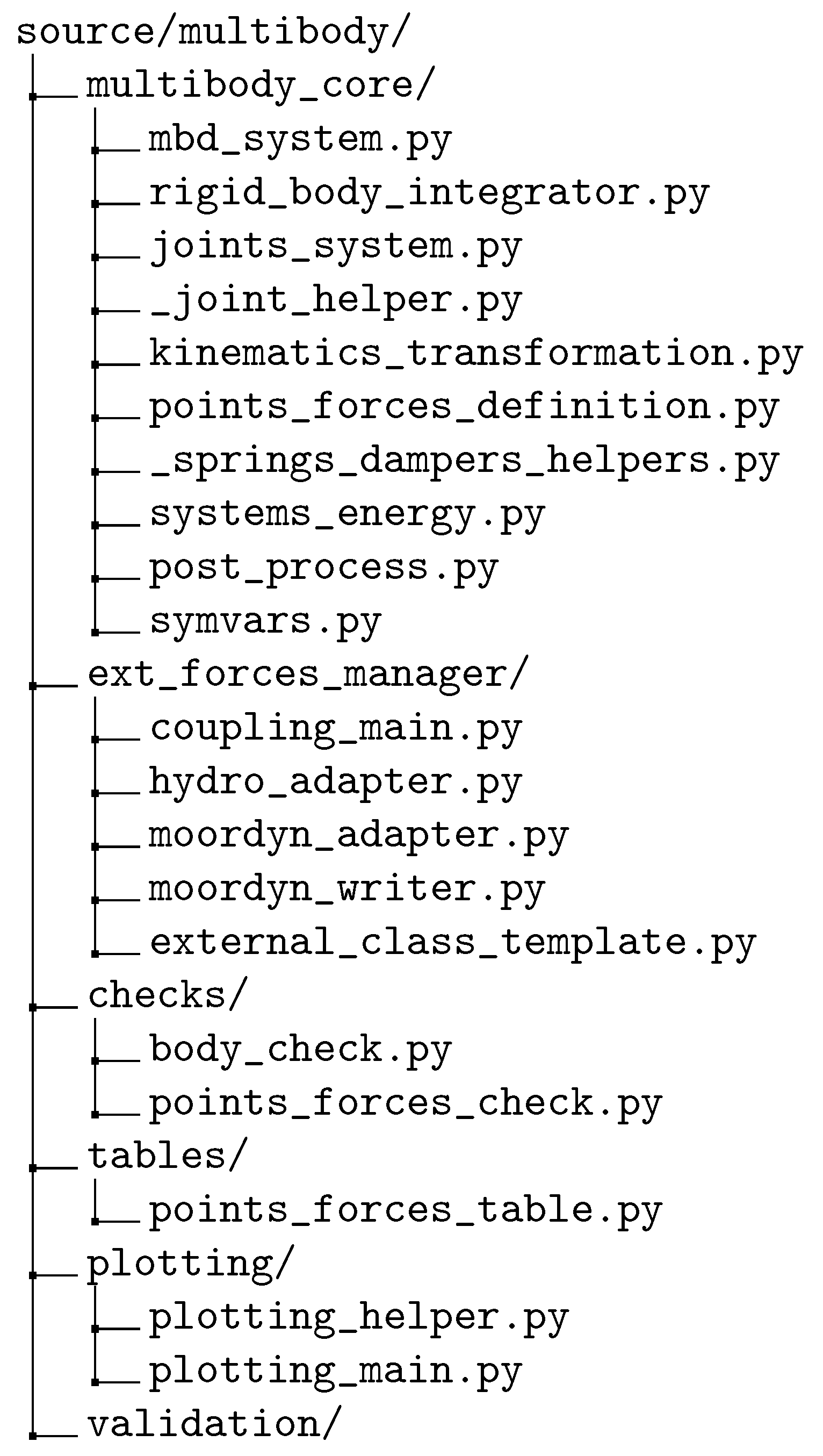
After describing the main workflow and public API, we now detail the overall code organization to provide a clear map of how the previously discussed classes and methods are structured, thereby facilitating community contributions. Standard naming conventions are followed throughout the repository, and private files or methods are prefixed with an underscore (_) to indicate components intended for internal use. The folder structure is shown in Figure 3 and the public API appears in Table 3.

With the module hierarchy clarified and the file structure outlined, we next introduce the public application programming interface (API) that is exposed when importing the M4E library, along with the corresponding locations where each component resides for further modification.

Table 3. Mapping of public API symbols to source files.

Symbol	Defined in
MbdSystem	multibody_core/mbd_system.py
integrate_dynamics	multibody_core/rigid_body_integrator.py
JointSystem, normalize_prismatic	multibody_core/joints_system.py
VelocityTransformation	multibody_core/kinematics_transformation.py
symvars_definition	multibody_core/symvars.py
points_force_finder	multibody_core/points_forces_definition.py
systems_energy	multibody_core/systems_energy.py
evaluate_trajectories	multibody_core/post_process.py
ExternalForcesManager	ext_forces_manager/coupling_main.py
checks (namespace)	checks/
plot (namespace)	plotting/
tables (namespace)	tables/

Table 3. Mapping of public API symbols to source files.

Symbol	Defined in
MbdSystem	multibody_core/mbd_system.py
integrate_dynamics	multibody_core/rigid_body_integrator.py
JointSystem, normalize_prismatic	multibody_core/joints_system.py
VelocityTransformation	multibody_core/kinematics_transformation.py
symvars_definition	multibody_core/symvars.py
points_force_finder	multibody_core/points_forces_definition.py
systems_energy	multibody_core/systems_energy.py
evaluate_trajectories	multibody_core/post_process.py
ExternalForcesManager	ext_forces_manager/coupling_main.py
checks (namespace)	checks/
plot (namespace)	plotting/
tables (namespace)	tables/

3.5. Qualitative Software Comparison

A wide range of open-source multibody dynamics (MBD) tools exists, each optimized for different objectives (e.g., contact simulation, large-scale constrained engineering models, robotics applications, or symbolic equation generation). To position M4E within this ecosystem, we provide a qualitative comparison against representative open-source frameworks (MBDyn, Chrono, MuJoCo, ODE, and PyDy) shown in

Table 4. Qualitative comparison of representative open-source MBD tools against M4E. “Symbolic EOM” indicates symbolic generation of equations of motion. “Analytical derivatives” indicates access to exact Jacobians from the governing equations (including AD ¹). “External coupling” indicates the ability to integrate external models without modifying the core solver and/or the presence of native multiphysics modules. “Coordinate reduction” indicates whether generalized/reduced coordinates are used.

Software	Symbolic	Analytical	Contact	External	Coordinate
	EOM	Derivatives		Coupling	Reduction
M4E v1	Yes	Yes	No	Yes	Yes
MBDyn v2.1	No	No	Limited	Yes	No
Chrono v9.0	No	No	Yes	Yes	No
MuJoCo v3.4	No	AD 1	Yes	No	Yes
ODE v0.11	No	No	Yes	No	No
PyDy v0.8	Yes	Yes	No	No	Yes

¹ AD is available via MJX (MuJoCo XLA) through JAX; MuJoCo itself is not inherently an AD framework.

. A quantitative benchmark (runtime, throughput, or maximum degrees of freedom) would be misleading in this context because (i) M4E currently targets a two-dimensional symbolic formulation, (ii) the tools are implemented in different languages (e.g., Python vs. C++), and (iii) their numerical goals differ substantially (e.g., contact-centric real-time simulation versus analysis-centric modeling). Therefore, the comparison below focuses on capabilities and workflows that are relevant to the intended use of M4E.

Several comparison dimensions require clarification beyond a binary table entry. First, Analytical derivatives refer to taking the derivative of the governing equations with respect to a symbolic variable, which directly supports linearization, sensitivity analysis, and gradient-based design.

Second, within external coupling, “Yes” indicates that the framework is designed to integrate external models (e.g., hydrodynamics, moorings, controllers, or other domain solvers) without modifying the core solver, either via a formal co-simulation API or via an adapter/plugin architecture. Additionally, some tools provide native multiphysics modules. Under this definition, M4E is explicitly designed for adapter-based coupling within the user workflow, whereas several engines are typically extended by linking against their library API or by co-simulation interfaces.

Third, contact support is selected because it often impacts solver design. Tools such as Chrono and MuJoCo incorporate sophisticated contact modeling frameworks, whereas M4E is currently positioned for mechanism dynamics and analysis workflows where contact is not the primary focus.

Finally, coordinate reduction is reported qualitatively rather than quantitatively. “Yes” indicates that the tool natively supports reduced (generalized/minimal) coordinate formulations, whereas “No” indicates that it primarily relies on maximal (absolute) coordinates with constraints enforced through algebraic relations.

3.6. Performance and Scaling Assessment

To assess the computational performance of M4E, we simulate an n-link planar pendulum with $n\in \{1,10,20,30,40,50,60\}$. Each link is modeled as a uniform rigid rod with length $L=2\mathrm{m}$ and mass of $10\mathrm{kg}$. Initially, all pendulums are horizontal and at rest. By keeping all physical parameters fixed and varying only n, this benchmark isolates how runtime and memory usage scale with the number of degrees of freedom. The measured runtimes and memory usage for all cases are summarized in

Table 5. Computational performance and memory usage for an n-link planar pendulum benchmark with fixed link length ($L=2$) using joint coordinates and RK45.

n	DOF	${\mathit{T}}_{\mathbf{sym}}$	${\mathit{T}}_{\mathbf{int}}$	Peak RSSsym	Peak RSSint
		[s]	[s]	[MB]	[MB]
1	1	0.298	0.072	202.34	204.11
10	10	0.741	3.188	208.00	208.57
20	20	1.333	19.084	213.55	214.43
30	30	2.458	40.085	218.88	220.47
40	40	3.937	81.702	226.48	226.99
50	50	6.172	141.56	230.29	232.98
60	60	8.341	245.876	239.25	243.07

.

Runtime: The total wall-clock runtime is divided into two stages:

• The symbolic stage includes the symbolic generation of the EOM of Equation (5) and compilation of the resulting expressions into executable functions using SymPy’s Lambdify tool. This stage is performed once per model and represents a one-time startup cost.
• The integration stage corresponds to solving the resulting system of ODEs for 30 s using the RK45 integrator with tolerances $(\mathrm{rtol},\mathrm{atol})=({10}^{-8},{10}^{-8})$. During time integration, the solver repeatedly calls the Lambdified functions to evaluate the system’s accelerations.

To quantify scaling behavior, the measured runtimes were fit using polynomial models. The symbolic runtime $T_{\mathrm{sym}}$ is well described by a quadratic dependence on n. The corresponding fit achieves a high coefficient of determination with $R^2\approx 0.998$ over the tested range, indicating excellent agreement with the measured data.

The integration time $T_{\mathrm{int}}$ exhibits a clear cubic dependence on n with a coefficient of determination $R^2\approx 0.999$ suggesting very strong cubic scaling. This scaling is consistent with solving the EOM with a dense mass matrix ${\mathit{B}}^T\mathit{M}\mathit{B}\in {\mathbb{R}}^{n\times n}$ at each solver step.

Memory: Memory usage is measured using the peak resident set size (peak RSS) of the Python process and is reported separately for the symbolic ($RS{S}_{\mathrm{sym}}$) and integration ($RS{S}_{\mathrm{int}}$) stages. Both of these values scale quadratically with a coefficient of determination of $R^2\approx 0.993$ and $R^2\approx 0.995$, respectively. For the benchmark sizes considered here, the additional memory used during time integration is modest (typically less than 1–2 MB beyond the symbolic peak).

3.7. Regression Tests and Documentation

Lastly, to ensure that developers’ modifications to the source code do not disrupt existing functionality, we provide two validation scripts in the validation module of the source tree: automated_validation.py and energy_and_ode.py. The first script verifies that the symbolic objects for CG positions, joint locations, the B matrix, and the $\dot{B}$ matrix remain consistent with a trusted reference. The second script integrates the system dynamics and computes the total energy at each time step, thereby testing the numerical portion of the implementation. This separation makes it straightforward to identify whether a failure arises from the symbolic formulation or the numerical integration.

The validation scripts can be executed with the following code:

Further details on the testing workflow and documentation are available in the GitHub repository [19,20].

4. Verification and Benchmarks

Along with any new computational tool comes a set of verification and benchmark tests designed to establish credibility and ensure that users can trust that the results are both accurate and reproducible. In this work, verification and benchmarking are divided into four main parts.

First, we compare the analytical EOM produced by M4E against a solved example from the literature. Once the analytical formulation is confirmed, we validate the time integration routines by comparing simulation results with those obtained using Chrono, an open-source physics engine [21].

Next, we conduct convergence studies to assess both the numerical stability of the M4E integrator and the solution convergence to Chrono results. Finally, we verify the external forces coupling library through a flexible pendulum example in which M4E is coupled with MoorDyn. Results are compared against both the analytical solution and a stand-alone M4E implementation to demonstrate consistency and interoperability.

4.1. Analytical Comparison

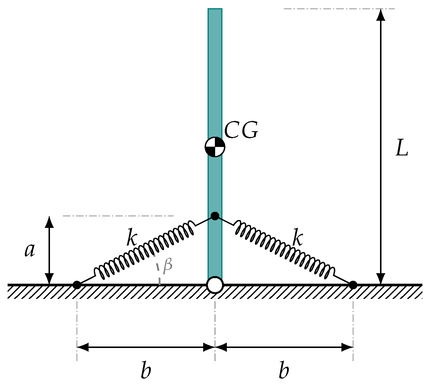
To verify the correctness of the symbolic formulation, we reproduce Example 7.13 in Ginsberg’s Advanced Engineering Dynamics textbook [22]. The goal is to find the stiffness matrix of the inverted pendulum shown in Figure 4 for small oscillations about its equilibrium. Using M4E, the EOM are

$$EOM={\displaystyle \frac{m_1{L}^2}{3}}\ddot{\theta }+\left[{\displaystyle \frac{2a^2{b}^{2}k{l}_0}{{(a^2+b^2)}^{3/2}}}-\frac{1}{2}{m}_{1}gL\right]\theta =0.$$

(6)

Consequently, the stiffness matrix K can be found in our code by taking ${\displaystyle \frac{\partial EOM}{\partial \theta }}$ at the equilibrium:

$$K=\left[{\displaystyle \frac{{\displaystyle 2k{l}_0{a}^2{b}^2}}{\sqrt{{(a^2+b^2)}^3}}}-\frac{1}{2}{m}_{1}gL\right].$$

(7)

For small oscillations, one can write

$$\cos \beta ={\displaystyle \frac{b}{\sqrt{a^2+b^2}}}.$$

(8)

Substituting Equation (8) into Equation (7) will result in the same expression found in the Ginsberg’s book.

4.2. Comparison to Chrono

After ensuring the correctness of the analytical EOM, we next verify that the numerical integration is performed correctly, i.e., that the code handles the numerical aspects of the dynamics accurately. To demonstrate integration accuracy and overall implementation correctness, we compare the results obtained with M4E to those from Chrono [21]. Three representative examples are used to illustrate code fidelity: a double pendulum, a double pendulum on a cart, and a two-dimensional version of the offshore wind platform SpiderFloat [23]. In Chrono, the Hilber–Hughes–Taylor (HHT) integrator is used with the default solver tolerance of ${10}^{-4}$. Unlike Chrono, M4E results in an ODE system; hence, constraint stabilization for drift corrections and its associated metrics are not applicable under the joint coordinate formulation. At the moment, M4E uses an explicit Runge–Kutta integration method. The fundamental difference in formulation, combined with the use of different integration schemes, can naturally lead to small cumulative deviations over time. To assess whether these differences are acceptable, we refer to the current literature [24,25,26].

The relative error metrics used for comparison follow the normalized root-mean-square error (RMSE) approach presented by Okada et al. [24], where an RMSE is computed for each body. We slightly modify this metric to prevent division by zero by adopting the normalization proposed by González et al. [25], where the normalization factor is the absolute maximum value of each coordinate or a minimum threshold equal to the integrator tolerance. This relative error formulation provides more robust insight into the simulation error even when the motion amplitude approaches zero, in contrast to the interpretation given by Ruggiu et al. [26]. The resulting metric is therefore a normalized RMSE (NRMSE) computed per body, defined below. Section 4.3 provides further discussion on integrator convergence and formulation implications.

$$\begin{array}{cc}\hfill e_{L2}^{\mathrm{rel}}\left(t\right)& ={\displaystyle \frac{|x^{\mathrm{M}4\mathrm{E}}\left(t\right)-x^{\mathrm{Ch}}\left(t\right)|}{{\max }_t\left(|x^{\mathrm{Ch}}\left(t\right)|,\mathrm{tol}\right)}},\hfill \end{array}$$

(9)

$$\begin{array}{cc}\hfill {\mathrm{NRMSE}}_b^{\left(i\right)}& =\sqrt{{\displaystyle \frac{1}{K}}\sum _{t=1}^K{\left(e_{L2}^{\mathrm{rel}}(t,i,b)\right)}^2},\hfill \end{array}$$

(10)

$$\begin{array}{cc}\hfill {\mathrm{NRMSE}}_b& =\sqrt{\sum _{i=1}^{N_{\mathrm{DOF}}}{\left({\mathrm{NRMSE}}_b^{\left(i\right)}\right)}^2}.\hfill \end{array}$$

(11)

4.2.1. Double Pendulum

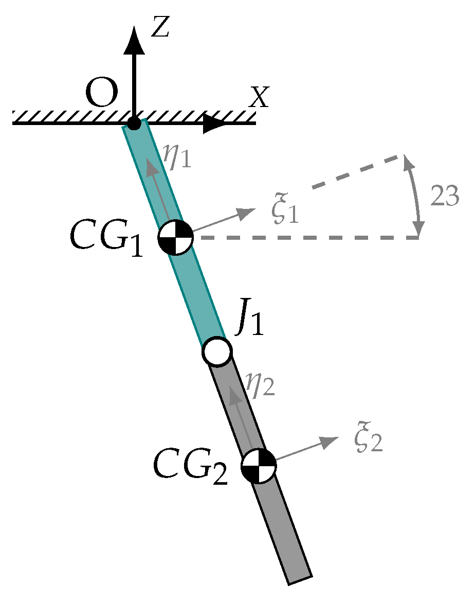
The double pendulum represents a canonical chaotic multibody system. To avoid diverging solutions, the double pendulum needs to be evaluated in the linear regime, i.e., small oscillations. In this test case, both pendulums are initially positioned at an angle of $23°$ with respect to the vertical. No external forces or initial velocities are applied. Each link is one meter long, with its center of gravity located at the center, as illustrated in Figure 5. A detailed description of how this system is modeled in M4E is provided in Section 5.2.

The simulation is executed for a total duration of $30 \mathrm{s}$ in both frameworks. M4E uses RK45 scheme with a reporting time step of $\Delta t=0.001 \mathrm{s}$, whereas Chrono uses the HHT integrator with a fixed time step of $\Delta t=0.0001 \mathrm{s}$.

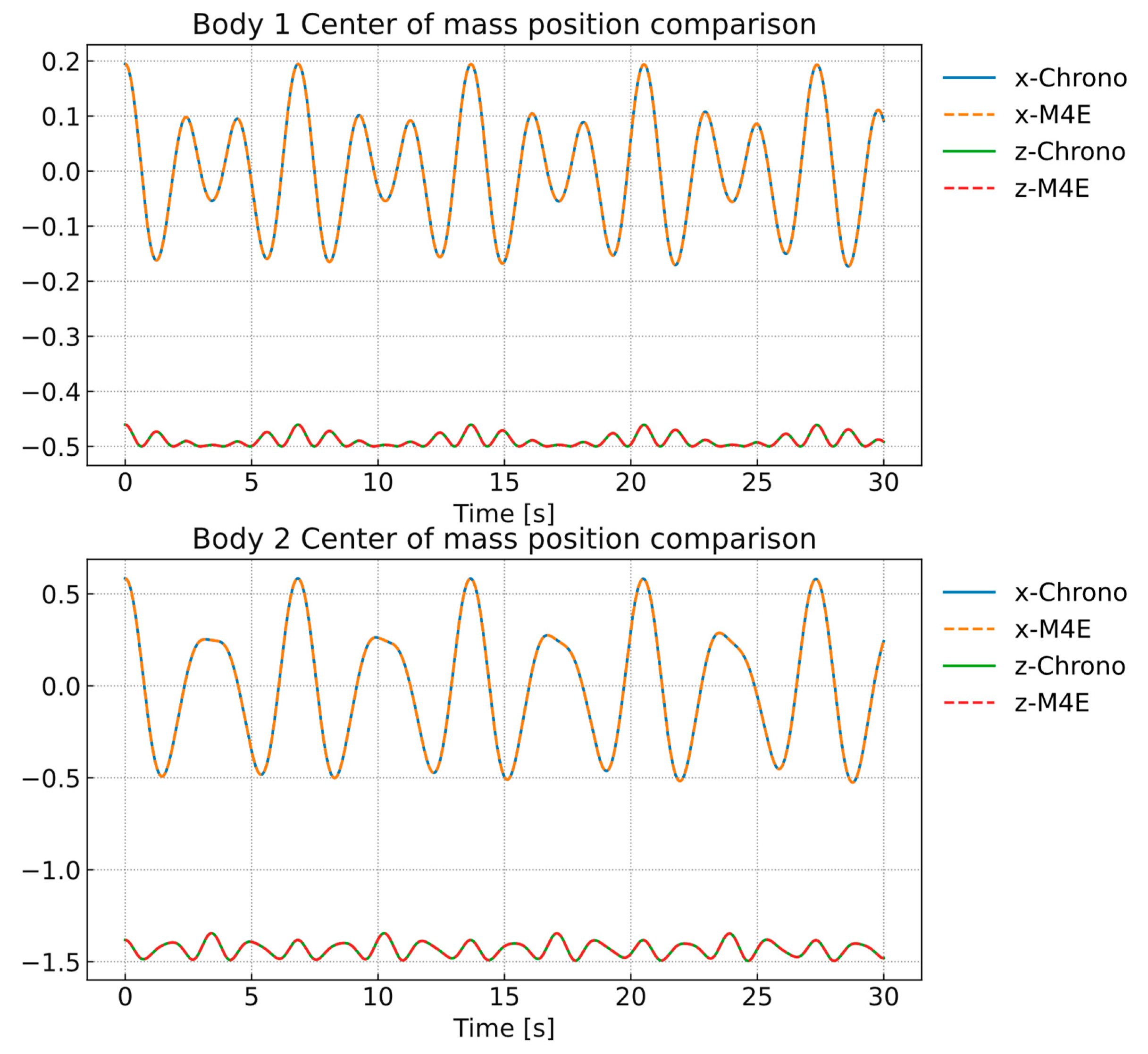
Figure 6 compares the time evolution of the center of gravity coordinates for both pendulum links. Solid lines correspond to Chrono, and dashed lines represent M4E. The output reporting interval for both tools is $0.01 \mathrm{s}$. Upon visual inspection, the trajectories produced by both frameworks are nearly indistinguishable. A quantitative error analysis is therefore carried out below.

When reporting accuracy metrics, both Ruggiu et al. [26] and González et al. [25] distinguish between two accuracy thresholds. The most restrictive tolerance, referred to as the high-accuracy level, is $2\times {10}^{-4}$ and is adopted here as the target accuracy. Although the error formulations differ slightly from Okada et al. [24], the modified metric is generally more restrictive, making it more challenging to meet the same tolerance level.

Table 6. Double pendulum simulation error metrics using Chrono as the reference.

Body	NRMSEb
1	$3.6\times {10}^{-6}$
2	$3.0\times {10}^{-6}$

reports the NRMSE for each body. In both cases, the NRMSE remains below the integration tolerance and within González’s high-accuracy criterion, confirming that the results obtained with M4E are consistent and accurate.

4.2.2. Double Pendulum on a Cart

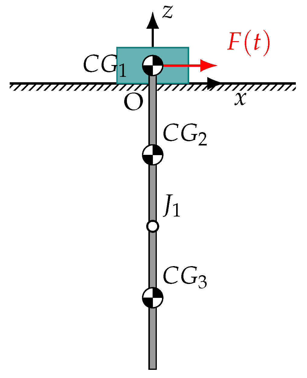
The next verification example increases the system complexity by introducing a prismatic joint and a time-dependent external force. A sinusoidal force is applied to the slider’s CG and is defined as

$$F\left(t\right)=3\cos \left(1.5t\right).$$

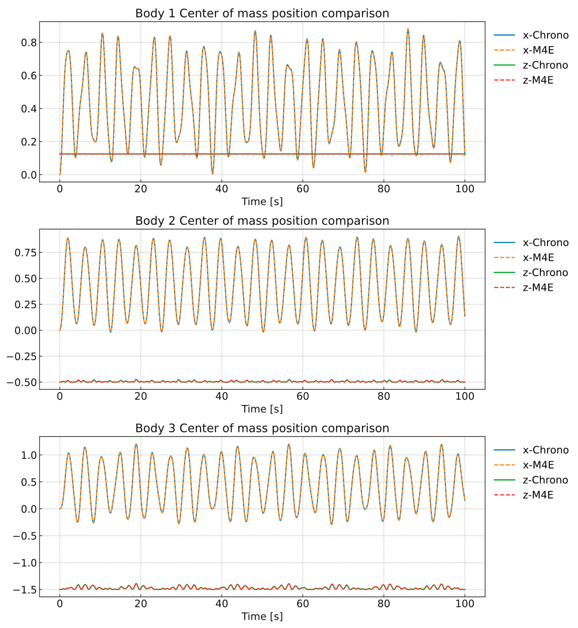
The simulation is run for $100 \mathrm{s}$ using the same time-stepping and reporting intervals as in the previous case. Figure 7 illustrates the multibody system.

The results are presented in the same format as the previous validation case: a figure showing the time evolution of each body’s CG coordinates, followed by a table summarizing the normalized error between both frameworks. As observed in Figure 8, the trajectories obtained from Chrono and M4E are visually indistinguishable, demonstrating close agreement throughout the entire simulation.

The computed NRMSE values, listed in

Table 7. Slider with double pendulum simulation error metrics using Chrono as the reference.

Body	NRMSEb
1	$3.3\times {10}^{-5}$
2	$3.2\times {10}^{-5}$
3	$2.4\times {10}^{-5}$

, are all below the previously established accuracy threshold ($2\times {10}^{-4}$), further confirming the numerical consistency of M4E. It is worth noting that the small error observed for the first body arises entirely from its x–component, as the z–direction has a constant value for all time steps. This shows that M4E naturally satisfies holonomic constraints without the need for explicit constraint stabilization.

4.2.3. SpiderFLOAT with Sliders

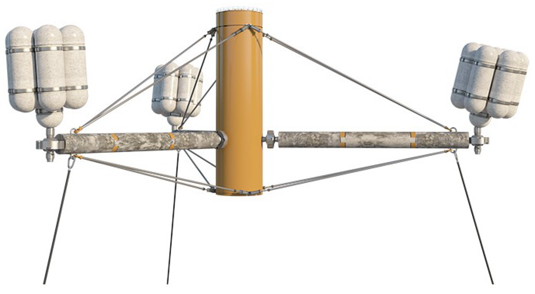
The SpiderFLOAT system, shown in Figure 9, is a conceptual design developed to enable cost-efficient deployment of offshore floating structures [23]. It consists of a central floating platform connected to several articulated legs, each connected to buoys, thus providing stability and buoyancy. In the present example, a sliding body (arm) is introduced between the legs and the buoys to provide active stability control.

A sinusoidal load of unit amplitude and frequency is applied at the central body. Additional sinusoidal excitations, with the same properties as the previous one, are applied along the sliding joints to enforce motion. Additionally, translational and rotational spring-damper elements are included in the model. This complex example is selected to evaluate whether M4E can correctly handle floating joints as well as translational and rotational DOFs.

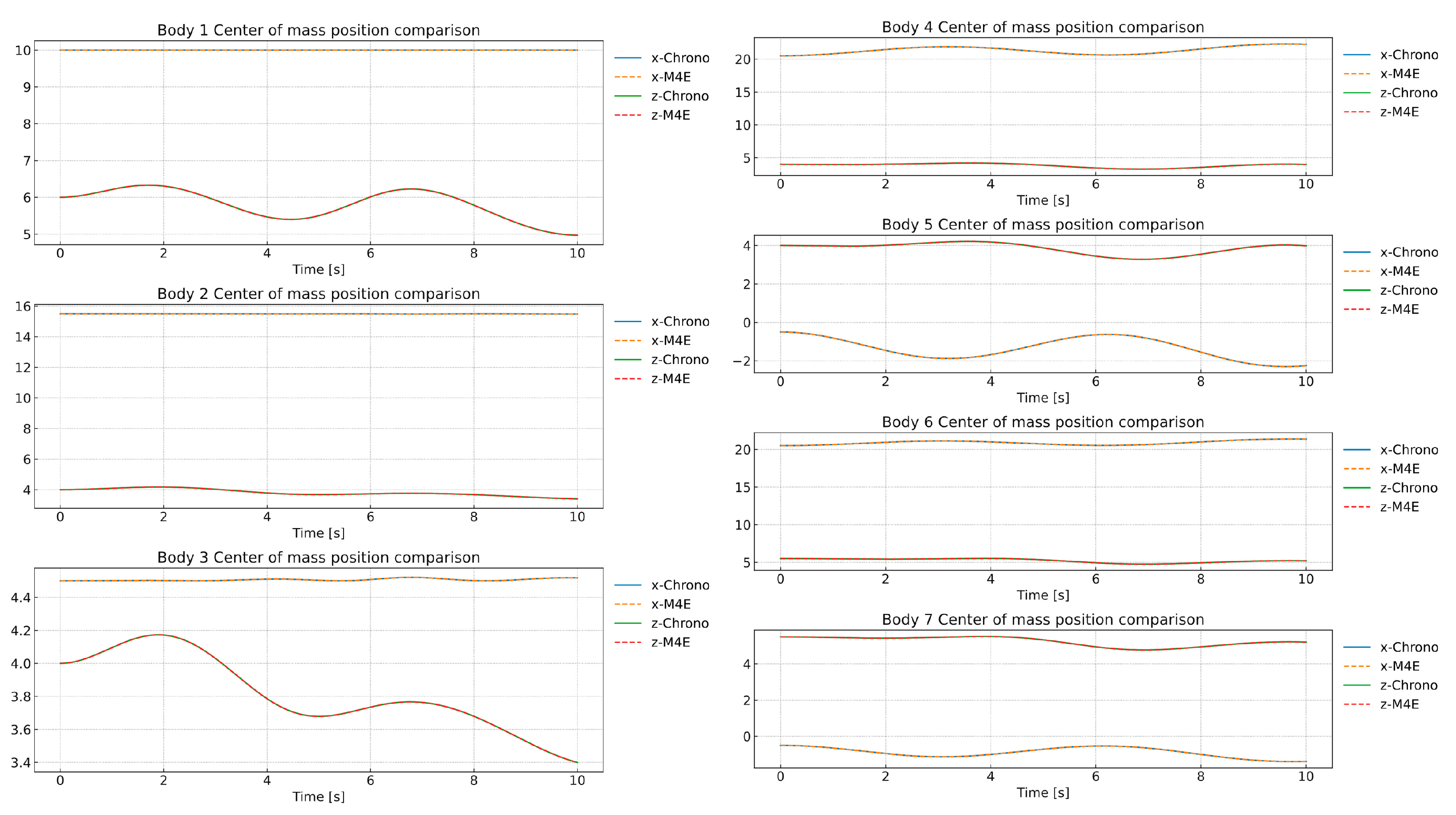
For the SpiderFLOAT validation, the center-of-gravity coordinates were divided into two subplots for clarity. A 10 s simulation was performed, and Figure 10 shows excellent agreement between Chrono and M4E for all bodies and coordinates.

The NRMSE values, summarized in

Table 8. SpiderFLOAT simulation error metrics using Chrono as the reference.

Body	NRMSEb
1	$1.4\times {10}^{-6}$
2	$1.2\times {10}^{-6}$
3	$1.2\times {10}^{-6}$
4	$3.2\times {10}^{-6}$
5	$2.8\times {10}^{-5}$
6	$3.0\times {10}^{-6}$
7	$2.0\times {10}^{-5}$

, confirm that even for this highly coupled, multi-joint configuration, the agreement between Chrono and M4E remains well within the prescribed accuracy tolerance.

Across the three validation cases presented—double pendulum, slider with double pendulum, and SpiderFLOAT—the numerical treatment and integration procedures in M4E are shown to be robust and consistent. All the tested joint types (revolute, prismatic, and floating), as well as the symbolic time-dependent loads, springs, and dampers, behave as expected. The following sections address convergence studies and the validation of the ExternalForcesManager module.

4.3. Convergence Studies

This section aims to demonstrate two key aspects of the integrator performance: (i) how the error of the solver library diminishes as the integrator absolute and relative tolerances are reduced, and (ii) how M4E and Chrono solutions converge as we refine the time integration tolerance by comparing the final position of the second pendulum in the double pendulum on a cart problem.

It is standard practice, in problems involving numerical time integration, to conduct convergence studies [27], verifying that the integration scheme exhibits the expected order of accuracy and that the numerical error decreases in a predictable manner. Currently, M4E supports only explicit integration schemes, implemented through the scipy.integrate.solve_ivp library. The default solver is the RK45 method, which is based on the Dormand–Prince algorithm [28].

We evaluate convergence by progressively tightening the absolute and relative tolerances of the integrator and comparing each simulation to the reference solution corresponding to the smallest tolerance pair $(\mathrm{rtol},\mathrm{atol})=({10}^{-12},{10}^{-15})$. The tolerance sets used are listed in

Table 9. Relative and absolute tolerances used in the convergence study for the slider with double pendulum problem.

rtol	${10}^{-4}$	${10}^{-6}$	${10}^{-8}$	${10}^{-10}$	${10}^{-12}$
atol	${10}^{-7}$	${10}^{-9}$	${10}^{-11}$	${10}^{-13}$	${10}^{-15}$

.

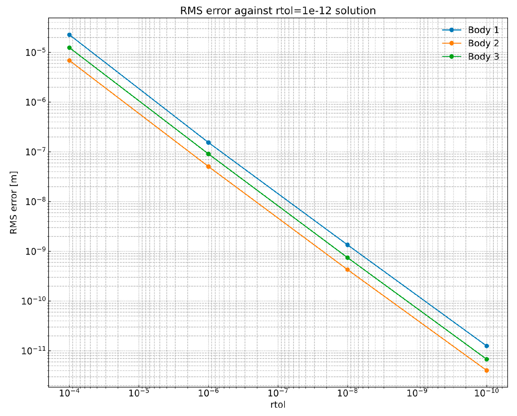
The RK45 integrator exhibits a first-order convergence trend when plotted in logarithmic scale. For each tolerance pair, we performed a simulation and computed the NRMSE for each body relative to the reference solution. The results in Figure 11 show a clear alignment of the data points, confirming that the error decreases consistently as the tolerances are reduced.

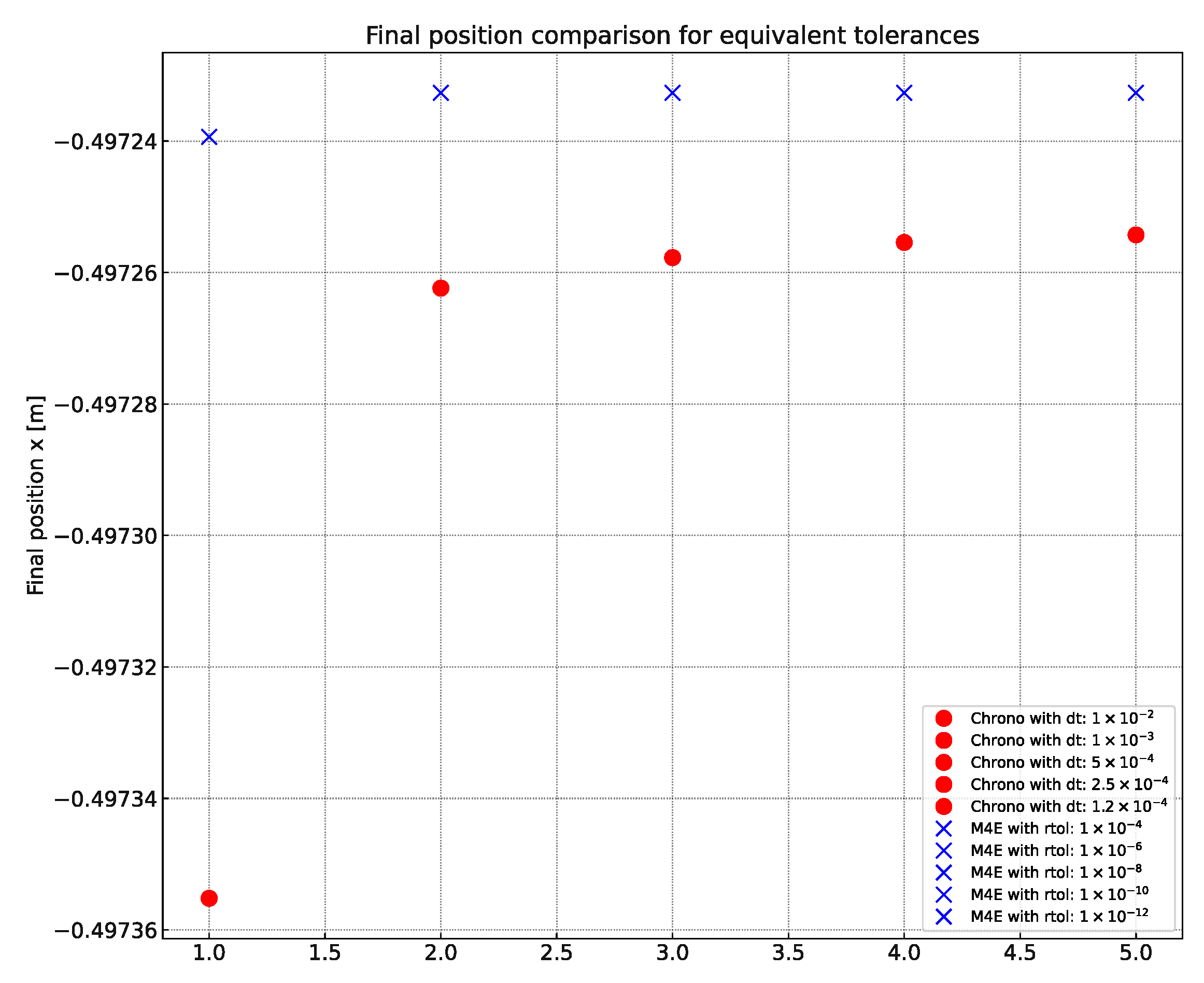
In addition, we compare M4E results with those obtained using Chrono. The comparison is performed using the z-coordinate of the first pendulum’s CG at the final time point. For M4E, the results correspond to the tolerance levels listed above, whereas for Chrono, the accuracy is increased by reducing the integration time step. As shown in Figure 12, the two solutions converge toward each other as the tolerances and time steps are refined.

As the precision is increased in both frameworks, the distance between the final solutions decreases, as summarized in

Table 10. Difference in the final z-coordinate of the first pendulum between M4E and Chrono for decreasing tolerance/time-step levels.

Case ID	Difference
1	$1.16\times {10}^{-4}$
2	$2.97\times {10}^{-5}$
3	$2.51\times {10}^{-5}$
4	$2.28\times {10}^{-5}$
5	$2.16\times {10}^{-5}$

. The residual differences are attributed to the distinct formulations discussed in Section 2 (joint coordinate method in M4E versus Newton–Euler equations in Chrono) and to the different numerical integration schemes used. Overall, the results confirm that M4E exhibits consistent and reliable convergence behavior.

4.4. Verification of External Tool Coupling: Flexible Pendulum Example

The final verification section checks the accuracy of the ExternalForcesManager class, which enables the coupling of M4E with external physics libraries. For this purpose, we use MoorDyn [29], a widely used open-source tool for modeling mooring line dynamics. A mooring line can be represented as a series of lumped-mass spring-damper segments. In the present test, we select a single-segment line, such that the mooring line behaves equivalently to a single linear spring, following the pendulum example from [30].

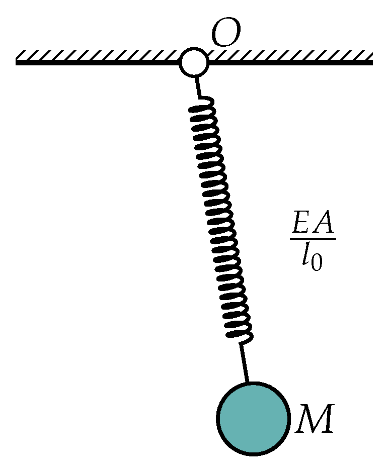
The verification system is a flexible pendulum consisting of a point mass suspended from the ground by a spring of stiffness $EA/l_0$, where E is Young’s modulus, A is the cross-sectional area, and $l_0$ is the undeformed length of the line (see Figure 13). The objective is to compare the dynamic response predicted by (i) the analytical solution, (ii) a stand-alone M4E model with a spring element, and (iii) an M4E model coupled with MoorDyn through the ExternalForcesManager. The comparison focuses on three characteristic motion periods: the horizontal oscillation period, $T_x$; the low-frequency vertical period, $T_{zL}$; and the high-frequency vertical period, $T_{zH}$.

The horizontal motion period, $T_x$, follows the classical harmonic pendulum expression:

$$T_x=2\pi \sqrt{{\displaystyle \frac{l_0}{g}}}.$$

(12)

For small-angle motion, the low-frequency vertical motion period is approximately half of the horizontal period:

$$T_{zL}\approx {\displaystyle \frac{T_x}{2}}.$$

(13)

Finally, the high-frequency vertical motion period, $T_{zH}$, corresponds to the natural frequency of the spring–mass system:

$$T_{zH}=2\pi \sqrt{{\displaystyle \frac{M}{K}}},$$

(14)

where M is the suspended mass and K is the spring stiffness, which for a mooring line is given by $K=EA/l_0$. All results are summarized in

Table 11. Comparison of period, in seconds, between the analytical solution, the flexible pendulum defined in M4E, and the flexible pendulum in M4E and MoorDyn.

Period (s)	Horizontal Motion	Vertical Motion (Low Freq.)	Vertical Motion (High Freq.)
Analytical	20.114	10.057	0.630
M4E	20.050	10.080	0.620
M4E + MD	20.250	10.080	0.620

and

Table 12. Percent error in period for the flexible pendulum defined in M4E and the flexible pendulum using M4E with MoorDyn.

Period Error	Horizontal Motion	Vertical Motion (Low Freq.)	Vertical Motion (High Freq.)
M4E (%)	0.319	0.228	1.57
M4E + MD (%)	0.675	0.228	1.57

.

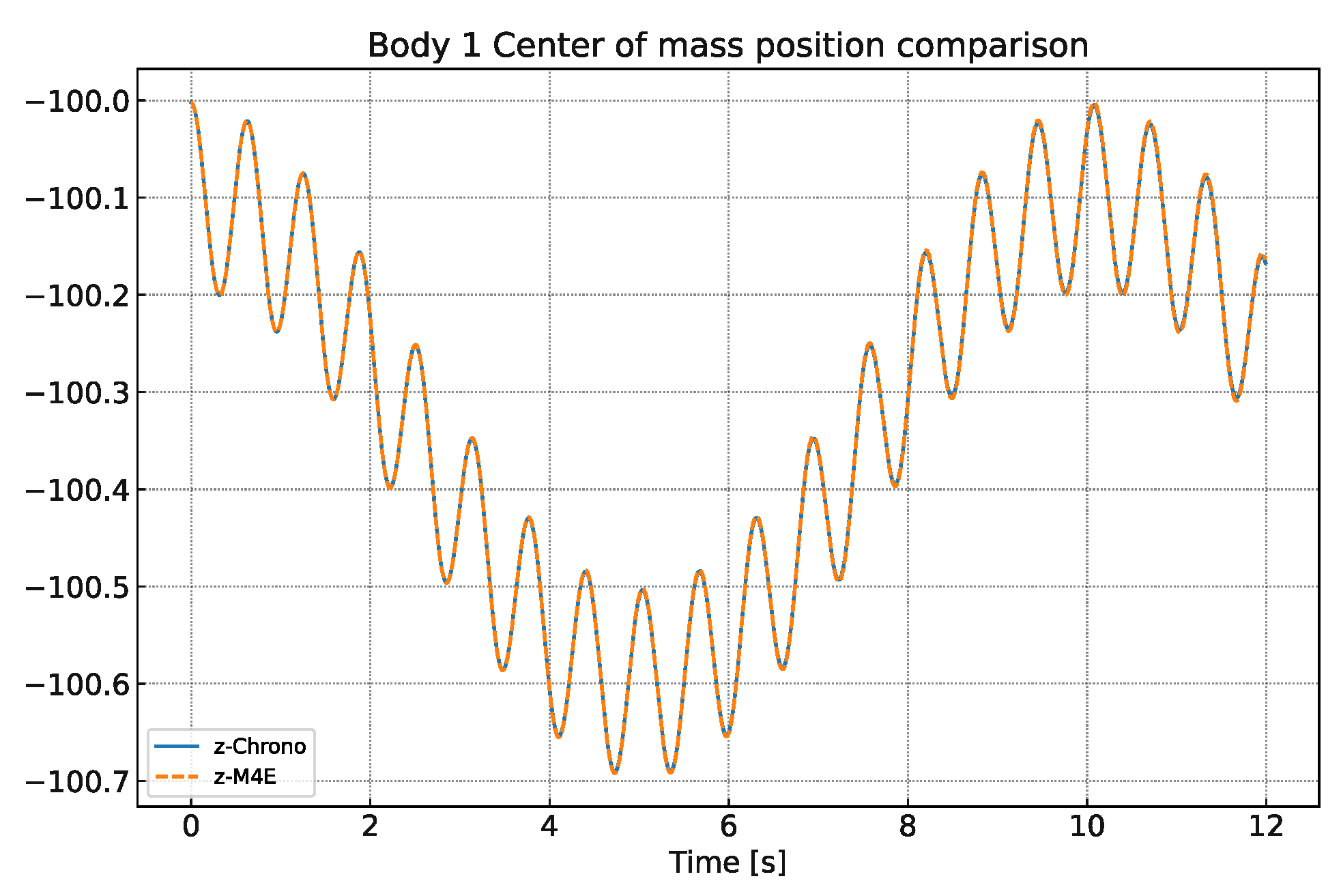
The tabulated data show good agreement between the simulation and analytical predictions. Both the pure M4E implementation and the M4E–MoorDyn coupled simulation produce nearly identical values for the vertical oscillation periods, confirming the correctness of the coupling interface. Figure 14 presents the vertical displacement response over a 12 s simulation, showcasing the close match between the two implementations across time.

5. Examples and Tutorials

This section aims to briefly demonstrate the simplicity of defining an example in M4E, rather than providing an in-depth explanation of the process. Detailed documentation is available in the GitHub repository [19,20]. Accordingly, we present two examples: a simple double pendulum and a more complex version of the SpiderFLOAT device [23].

5.1. Double Pendulum Example

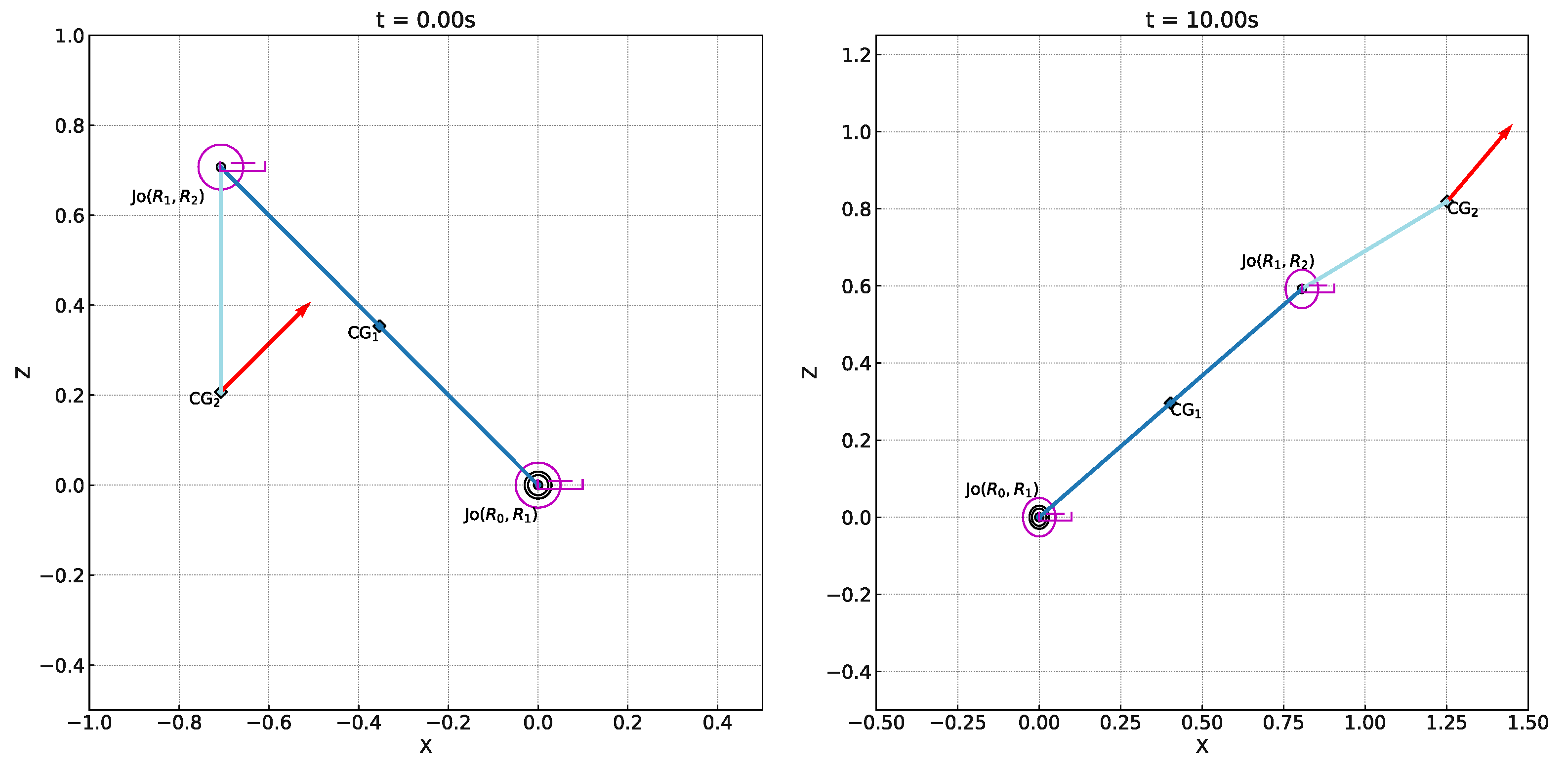
We begin by modeling and simulating a double pendulum system, initialized as shown in Figure 15. This process is organized into four main components: (i) geometry definition, (ii) forces definition, (iii) initial conditions, and (iv) simulation parameters.

The geometry block provides the information needed to assemble the multibody system in its initial configuration. It first specifies the origin of the reference frame. Then, for each joint, it provides the joint type: F (floating), R (revolute), or P (prismatic). This is followed by a list of the parent and child bodies connected by each joint. The vectors that connect the parent body’s center of gravity (CG) to the joint and the joint to the child body’s CG are also provided, as discussed in Section 3.1.

The following geometry input can be used to define a double pendulum:

M4E automatically generates a table similar to the one provided in Figure 2 to help the user better visualize the geometry input shown in

Table 13. Output table for double pendulum bodies configuration.

Joint	Connected Bodies	Joint Type	ParentCGtoJoint	JointtoChildCG	Prismatic Direction
1	0 1	R	[0, 0]	[0, −0.5]	[NaN, NaN]
2	1 2	R	[0, −0.5]	[0, −0.5]	[NaN, NaN]

.

A force of 28.2 N is applied at the center of gravity of the second link, oriented at an angle of 45 degrees in the absolute frame. A torsional spring with an undeformed angle of −135 degrees, in the pendulum frame, is introduced at the first revolute joint, and torsional dampers are added at each joint. The definitions of these force elements are provided below.

The initial condition vector contains both position and velocity components for all joint coordinates. These coordinates can be accessed in MbdSys.Q and MbdSys.QD, which for this example take the values [Theta_1,Theta_2] and [ThetaD_1,ThetaD_2], respectively.

For this example, the initial joint coordinates are set to 135 degrees and 0 degrees, respectively. An initial angular velocity of $0.4\mathrm{rad}/\mathrm{s}$ is prescribed to the upper link in the negative y-direction:

The remaining parameters define the physical and numerical settings of the simulation. These include the time step, total simulation time, gravitational acceleration, body masses, and inertias. The array gVec allows the user to scale the effect of gravity on individual bodies, if desired. Optional parameters control visualization and animation output.

Using the definition above, M4E constructs the double pendulum configuration shown in Figure 15, corresponding to the initial time instant $t=0$.

5.2. SpiderFLOAT

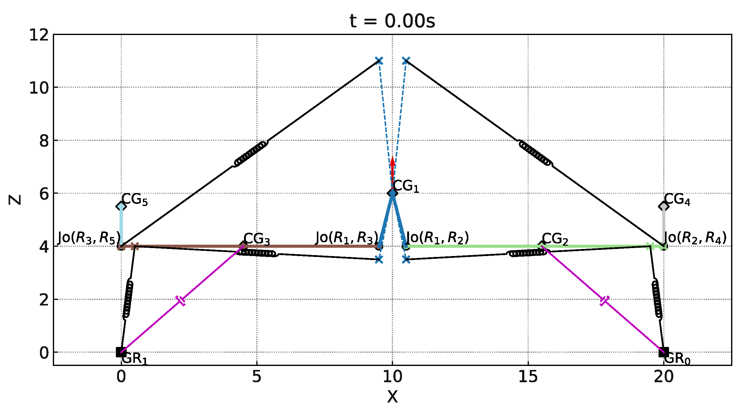
The mechanical topology of the system comprises a main floating body followed by a symmetric distribution of articulated legs. Each leg is attached to the central platform through a revolute joint and terminates in an arm that can extend along its local x-direction via a prismatic joint. A buoy is then connected to the far end of each arm through a revolute joint, providing restoring forces in pitch and heave.

The force definitions rely on identifying the application points for all spring, damper, and body-force elements. Points attached to the ground (GR) are fixed points, whereas body-attached points (BD) move with the rigid body to which they belong. These points are first defined as follows:

After the points definition, external forces are assigned by referencing these locations and defining additional parameters, such as force components, spring stiffness and undeformed length, and damper coefficient. These quantities can be expressed either numerically or symbolically, allowing for efficient parameter studies.

Figure 16 illustrates the initial configuration and body connectivity of the SpiderFLOAT system at $t=0$.

6. Linearization, Optimization, and Control

Linearization, optimization, and control capabilities are not part of the current software release, as the primary objective of this work is to introduce a user-friendly symbolic simulation framework. Nevertheless, the proposed architecture is explicitly designed to support these advanced analyses, and a brief overview of how they can be achieved is provided below.

First, linearization can be performed by applying a first-order Taylor expansion to the equations of motion and evaluating them about a chosen configuration. In the Ginsberg validation example (Section 4.1), we demonstrated how SymPy enables automatic differentiation to compute system series, such as the stiffness matrix, directly from the symbolic equations of motion. This capability naturally extends to the construction of linearized state-space models.

Second, gradient-based optimization is enabled through the symbolic formulation of the governing equations. Both MATLAB Symbolic Toolbox and SymPy provide native support for Jacobian and sensitivity calculations. Combined with the ability to parameterize system properties—including masses, joint locations, and force-element parameters—this framework allows for efficient, fully differentiable parametric optimization workflows.

Finally, controller design is facilitated through the external force manager described in Section 3.2.2. This module allows users to apply arbitrary external forces and moments during simulation while providing access to the system’s equations of motion, as well as its positions, velocities, and accelerations. These features can be directly leveraged for the implementation and evaluation of custom linear or nonlinear control strategies.

7. Limitations and Future Work

Currently, the developed code only supports modeling two-dimensional systems. Work on three-dimensional modeling is ongoing and is expected to be released in 2026. Flexible multibody systems can be modeled using the finite segment method, in which a flexible system is divided into a set of rigid bodies connected via kinematic joints [2,31,32,33]. Modeling systems with kinematically closed chains is not directly supported; however, the user can convert a closed-chain system into an open-chain one using the cut-joint method to generate the closed-chain EOM [3]. Direct modeling of closed-chain systems and inclusion of nonholonomic constraints will be provided in future versions.

8. Conclusions

This work introduces a user-friendly multibody dynamics framework that generates analytical EOM for applications in simulation, design exploration, control, and optimization. The proposed tool is highly versatile, suitable for applications in robotics, control, and design. Moreover, it incorporates integrated external libraries that enable modeling of offshore systems such as underwater robotics systems and marine energy converters.

A key feature of this open-source library is that it requires no prior expertise in multibody dynamics. Users only need to specify the geometry and connectivity of their system by defining center of gravity locations and joint vectors. Another major strength lies in its modular and extensible architecture. Through the ExternalForcesManager class, users can seamlessly integrate additional physical domains and external solvers, such as hydrodynamics or mooring dynamics, without embedding everything into a single monolithic code base. This design philosophy enhances reusability, clarity, and interoperability across physics-based libraries.

The symbolic formulation, combined with the joint coordinate representation, enables rapid parametric studies and efficient design-space exploration. The symbolic architecture also facilitates system linearization, frequency domain analysis, and gradient-based optimization.

The framework has been validated at multiple levels. First, the symbolic EOM were benchmarked against textbook examples [22]. Second, the numerical integration results were compared to Project Chrono simulations [21]. Finally, the external coupling capabilities were verified through MoorDyn [29] integration and comparison with analytical solutions.

Future developments will focus on extending the formulation to three-dimensional systems, advancing the linearization and frequency domain modules, including new kinematic constraints, integrating the EOM with physics-informed machine learning tools, and enabling gradient-based optimization for efficient design exploration. Together, these efforts aim to make the framework robust and extensible and create the foundation for multiphysics simulation and design in renewable energy and beyond.

9. Availability/Reproducibility

This library is publicly available on GitHub [19,20]. The repository includes detailed installation instructions and guidance for building the local documentation in both PDF and website formats. The documentation provides example workflows and developer guidelines to facilitate community use and contribution.

All examples presented in this paper are included in the repository to ensure full reproducibility of the results.

References

- Gede, G.; Peterson, D.L.; Nanjangud, A.S.; Moore, J.K.; Hubbard, M. Constrained multibody dynamics with Python: From symbolic equation generation to publication. In Proceedings of the International Design Engineering Technical Conferences and Computers and Information in Engineering Conference, Portland, OR, USA, 4–7 August 2013; Volume 55973, p. V07BT10A051. [Google Scholar]
- Nikravesh, P. Planar Multibody Dynamics: Formulation, Programming with MATLAB®, and Applications; CRC Press: Boca Raton, FL, USA, 2018. [Google Scholar]
- Nikravesh, P.E. Systematic reduction of multibody equations of motion to a minimal set. Int. J. Non-Linear Mech. 1990, 25, 143–151. [Google Scholar] [CrossRef]
- Nikravesh, P.E.; Gim, G. Systematic Construction of the Equations of Motion for Multibody Systems Containing Closed Kinematic Loops. In Proceedings of the 15th ASME Design Automation Conference, Montreal, QC, Canada, 17–21 September 1989. [Google Scholar]
- Kane, T.R.; Levinson, D.A. Dynamics: Theory and Applications; McGraw-Hill: New York, NY, USA, 1985. [Google Scholar]
- Jerkovsky, W. The Structure of Multibody Dynamics Equations. J. Guid. Control Dyn. 1978, 1, 173–182. [Google Scholar] [CrossRef]
- Nikravesh, P.E. Computer-Aided Analysis of Mechanical Systems; Prentice-Hall, Inc.: Hoboken, NJ, USA, 1988. [Google Scholar]
- Tasora, A.; Serban, R.; Mazhar, H.; Pazouki, A.; Melanz, D.; Fleischmann, J.; Taylor, M.; Sugiyama, H.; Negrut, D. Chrono: An open source multi-physics dynamics engine. In International Conference on High Performance Computing in Science And Engineering; Springer: Cham, Switzerland, 2015; pp. 19–49. [Google Scholar]
- Tasora, A. Numerical Methods for Large-Scale Multibody Problems—Lecture (Milano, February 2020). 2020. Available online: https://www.projectchrono.org/tasora/download/lecture_milano_mb_feb_20.pdf (accessed on 30 September 2025).
- The MathWorks, Inc. How Simscape Models Represent Physical Systems. Available online: https://www.mathworks.com/help/simscape/ug/how-simscape-models-represent-physical-systems.html?utm_source=chatgpt.com (accessed on 30 September 2025).
- Hall, M. MoorDyn User’S Guide; Department of Mechanical Engineering, University of Maine: Orono, ME, USA, 2015; Volume 15. [Google Scholar]
- Ancellin, M.; Dias, F. Capytaine: A Python-based linear potential flow solver. J. Open Source Softw. 2019, 4, 1341. [Google Scholar] [CrossRef]
- Sabet, S. Analytical Modeling, Control, Energy Analysis, and Path Planning of Spherical Robots. Ph.D. Thesis, The University of Arizona, Tucson, AZ, USA, 2021. [Google Scholar]
- Nikravesh, P.E. An overview of several formulations for multibody dynamics. In Product Engineering; Springer: Dordrecht, The Netherlands, 2005; pp. 189–226. [Google Scholar]
- Gim, G.; Nikravesh, P.E. Joint Coordinate Method for Analysis and Design of Multibody Systems: Part 1. System Equations. KSME J. 1993, 7, 14–25. [Google Scholar] [CrossRef]
- Gim, G.; Nikravesh, P.E. Joint Coordinate Method for Analysis and Design of Multibody Systems: Part 2. System Topology. KSME J. 1993, 7, 26–34. [Google Scholar] [CrossRef]
- McPhee, J.J. On the use of linear graph theory in multibody system dynamics. Nonlinear Dyn. 1996, 9, 73–90. [Google Scholar] [CrossRef]
- Meurer, A.; Smith, C.P.; Paprocki, M.; Čertík, O.; Kirpichev, S.B.; Rocklin, M.; Kumar, A.; Ivanov, S.; Moore, J.K.; Singh, S.; et al. SymPy: Symbolic computing in Python. PeerJ Comput. Sci. 2017, 3, e103. [Google Scholar] [CrossRef]
- Diaz-Flores, A.; Sabet, S. M4E: Multibody for Everybody: A User-Friendly Multibody Dynamics Tool (Python). Available online: https://github.com/Project-SEA-Stack/Python_Multibody_for_Everybody (accessed on 8 December 2025).
- Sabet, S.; Diaz-Flores, A. M4E: Multibody for Everybody: A User-Friendly Multibody Dynamics Tool (MATLAB). Available online: https://github.com/Project-SEA-Stack/MATLAB_Multibody_for_Everybody (accessed on 8 December 2025).
- Team, P.C.D. Chrono: An Open Source Framework for the Physics-Based Simulation of Dynamic Systems. Available online: https://github.com/projectchrono/chrono (accessed on 9 October 2025).
- Ginsberg, J.H. Advanced Engineering Dynamics; Cambridge University Press: Cambridge, UK, 1998. [Google Scholar]
- National Renewable Energy Laboratory. SpiderFLOAT Spins a Web of Offshore Innovation. 2019. Available online: https://www.nrel.gov/news/detail/program/2019/spiderfloat-innovation (accessed on 12 October 2025).
- Okada, T.; Dong, S.; Kuzuno, R.; Takahashi, Y.; Shizuno, Y.; Hara, Y.; Otsuka, K.; Makihara, K. State observer of multibody systems formulated using differential algebraic equations. Multibody Syst. Dyn. 2024, 62, 401–431. [Google Scholar] [CrossRef]
- González, M.; Dopico, D.; Lugrís, U.; Cuadrado, J. A benchmarking system for MBS simulation software: Problem standardization and performance measurement. Multibody Syst. Dyn. 2006, 16, 179–190. [Google Scholar] [CrossRef]
- Ruggiu, M.; González, F. A benchmark problem with singularities for multibody system dynamics formulations with constraints. Multibody Syst. Dyn. 2023, 58, 181–196. [Google Scholar] [CrossRef]
- Bauchau, O. Flexible Multibody Dynamics; Solid Mechanics and Its Applications; Springer: Dordrecht, The Netherlands, 2011. [Google Scholar]
- Dormand, J.R.; Prince, P.J. A family of embedded Runge–Kutta formulae. J. Comput. Appl. Math. 1980, 6, 19–26. [Google Scholar] [CrossRef]
- Hall, M. MoorDyn V2: New Capabilities in Mooring System Components and Load Cases. In Proceedings of the ASME 2020 39th International Conference on Ocean, Offshore and Arctic Engineering (OMAE 2020), Golden, CO, USA, 3–7 August 2020. [Google Scholar]
- MoorDyn Development Team. MoorDyn: Open-Source Mooring Dynamics Model—Test Cases. 2025. Available online: https://github.com/FloatingArrayDesign/MoorDyn/tree/master/tests (accessed on 29 October 2025).
- Connelly, J.; Huston, R. The dynamics of flexible multibody systems: A finite segment approach—I. Theoretical aspects. Comput. Struct. 1994, 50, 255–258. [Google Scholar] [CrossRef]
- Connelly, J.D.; Huston, R.L. The dynamics of flexible multibody systems: A finite segment approach—II. Example problems. Comput. Struct. 1994, 50, 259–262. [Google Scholar] [CrossRef]
- Nikravesh, P.; Chung, I.; Benedict, R. Plastic hinge approach to vehicle crash simulation. Comput. Struct. 1983, 16, 395–400. [Google Scholar] [CrossRef]
Figure 2.
(Top) Representation of a wave energy converter composed of two flaps connected by revolute joints. (Bottom) Bodies configuration table.
Figure 3.
Source code modules structure of the multibody package v1 following PEP 8 (Python Enhancement Proposal) (accessed on 5 December 2025).
Figure 4.
A flap held by two springs, adapted from [
22].
Figure 5.
Double pendulum with both links rotated around the y-axis at .
Figure 6.
Time histories of the double pendulum 30 s simulation to compare between Chrono (solid lines) and M4E (dashed lines).
Figure 7.
Slider with double pendulum configuration at .
Figure 8.
Time histories for the slider with double pendulum 100 s simulation to compare Chrono (solid lines) and M4E (dashed lines).
Figure 9.
Schematic configuration of the
SpiderFLOAT system [
23].
Figure 10.
Time histories of SpiderFLOAT 10 s simulation to compare Chrono (solid lines) and M4E (dashed lines).
Figure 11.
M4E convergence history for the slider with double pendulum example using the Dormand–Prince integration algorithm.
Figure 12.
Comparison of M4E and Chrono convergence behavior for the slider double pendulum problem.
Figure 13.
Flexible pendulum example sketch.
Figure 14.
Z-coordinate of the flexible pendulum problem for the coupled MoorDyn with M4E (solid blue) and pure M4E using a spring (dashed orange).
Figure 15.
Double pendulum configuration at (left), and (right).
Figure 16.
SpiderFLOAT system configuration at .