1. Introduction
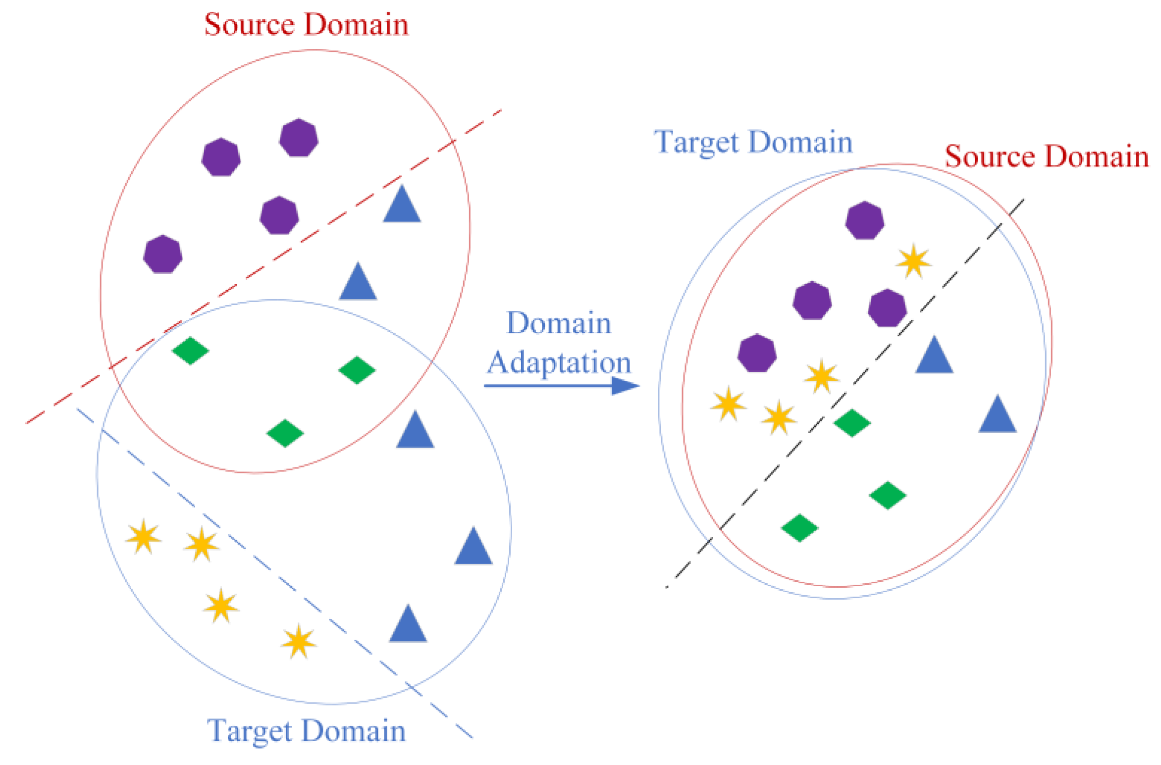
In recent years, big data technology has been extensively applied in the field of aero-engine fault diagnosis, with the most notable example being the integration of transfer learning into fault diagnosis methods. Fault diagnosis methods based on transfer learning can acquire shared knowledge from distinct, yet related tasks. This relaxes the constraint that the data in both the source and target domains must follow the same distribution, thereby reducing the reliance on highly accurate labeled fault data. This significantly broadens the generalization capability of fault diagnosis [
1,
2]. From the perspective of data sources, fault diagnosis methods for aero-engines based on transfer learning can be categorized into single-dimensional data fault diagnosis methods, multi-dimensional data fault diagnosis methods, and multi-source data fault diagnosis methods.
Single-dimensional data fault diagnosis methods use a sensor of the same type to collect data at one location, identify, and analyze the technical condition or degradation degree of the equipment. Zhang et al. [
3] addressed the issue of low diagnostic accuracy in engine fault diagnosis arising from limited fault feature data and highly variable operating conditions. Using a long short-term memory neural network with a wide convolutional kernel, they performed knowledge transfer on vibration data collected from the cylinder head, achieving high cross-domain fault diagnosis accuracy. Guo and Zhang [
4] employed a multi-scale and multi-view domain Adaptation network to develop a transfer learning method capable of addressing scenarios with insufficiently labeled data. The effectiveness of the proposed method was validated through simulation experiments using engine vibration data under seven operating conditions. Shen et al. [
5] proposed a hybrid transferability metric based on weighted correlation-diversity shift for the transfer learning of vibration data from aero-engines, thereby partially addressing the problem of cross-domain diagnostics under extreme class imbalance. Single-dimensional data fault diagnosis methods [
6,
7] have achieved some success, but in real applications, the operating conditions of aero-engines are complex. When faults occur, the data include multiple vibration excitation sources, component coupling, and information attenuation. Relying on a single information source will aggravate the uncertainty of fault diagnosis, which can easily lead to misdiagnosis, missed diagnosis, and expanded diagnosis scope. Generally, source domain data with high similarity to the target data must be selected for training. Therefore, multi-dimensional data fault diagnosis methods that can contain more fault features are born.
Multi-dimensional data fault diagnosis methods use sensors of the same type to collect data at different locations, identify, and analyze the technical condition or degradation degree of equipment. Ding et al. [
8] proposed a multitask Siamese network for diagnosing faults in aero-engine bearings. It uses both the axial and radial vibration data collected and, through a shared encoder, ensures similarity between the features of the two datasets, thereby solving the problem of low fault diagnosis accuracy with limited data. Shen et al. [
9] proposed a generative transfer learning fault diagnosis method, which involves collecting vibration data from both the cylinder block and output shaft of an aero-engine. It represents domain-invariant fault features through sparse matrices and domain-specific fault features using Gram matrices. This method demonstrates the separability of fault features and domain features within mechanical signals, thereby resolving cross-domain diagnosis challenges under extreme class imbalance conditions. Shen et al. [
10] proposed a transfer learning method based on cycle-consistent adversarial networks to address cross-domain fault diagnosis and missing label issues. The method is validated using vibration data collected from both the fan and driving ends of the engine, achieving a better fault diagnosis effect. Multi-dimensional data fault diagnosis methods [
11,
12] enhance data reliability compared with single-dimensional data fault diagnosis methods. However, because the data remain confined to the same dimensions, they fail to enrich the captured fault features. For instance, when gearbox wear occurs, oil spectral data are more useful than vibration data. Related research [
13] also indicates that multi-source data yield more reliable fault diagnosis results than single-source data.
Multi-source data fault diagnosis methods use different sensors to collect data at different locations, identify and analyze the technical condition or degradation degree of equipment. Zhu et al. [
14] selected the compressor flow rate, compressor efficiency, gas turbine flow rate, gas turbine efficiency, and power turbine efficiency as the research data. By training single-class support vector machines using source domain and target domain data, respectively, and considering the hyperplane differences between the source and target domains during training, the model can ensure strong generalization capabilities. It can achieve a high fault diagnosis performance even when the data are scarce or the target domain data volume changes significantly. Srinivaas et al. [
15] integrated transfer learning, federated learning, and deep neural networks to propose a federated learning method based on transformer-based deep-learning hybrid architectures. Through simulation experiments using vibration data and sound pressure data collected from two operating engines under different conditions, the results demonstrated a significant improvement in the accuracy and robustness of the model. Zhao et al. [
16] integrated support vector machines with transfer learning, enhancing the accuracy of fault diagnosis in the target domain by performing cross-domain learning on parameters such as the high/low-pressure rotor speed, fan/turbine outlet temperature, and compressor/turbine outlet pressures. Magliacano et al. [
17] proposed a full-thickness damage state model for carbon fiber composites, evaluating damage in the most stressed structural elements based on five classical failure criteria. This approach resolves the challenge of quantitatively analyzing and quantifying damage states in aircraft through-thickness damage using closed-form analysis. The multi-source data fault diagnosis methods described above [
18] suppose that the data are mutually independent, artificially weakening the complex nonlinear relationships among the various data. This is neither consistent with the mechanism of aero-engine failures nor conducive to achieving high fault diagnosis accuracy and stability in the model.
In summary, to address the issues of low accuracy and poor stability in aero-engine fault diagnosis caused by excessive discrepancies among multi-source data, this study proposed an Aero-Engine Fault Diagnosis Method based on DANN and Feature Interaction (FI-DANN). First, the fundamental theories related to feature interaction [
19,
20], CNN [
21,
22], and DANN [
23,
24] involved in this study are briefly introduced. Second, the mathematical representation, model construction, and training process of FI-DANN are analyzed. Finally, simulations were conducted using public datasets and fault data from a certain type of aero-engine, and the results were compared with the fault diagnosis algorithms of CNN and traditional DANN.
The remainder of this paper is organized as follows:
Section 2 discusses related works on feature interaction, CNN, and DANN.
Section 3 constructs and describes the proposed FI-DANN. In
Section 4, two case studies are used to evaluate the diagnostic performance of the proposed FI-DANN. Finally, the conclusions of this study are presented in
Section 5.
3. The Proposed Method
Although the introduction of transfer learning theory has significantly enhanced the accuracy of cross-domain fault diagnosis, which was previously difficult to improve, owing to inconsistent data distributions. However, as traditional transfer learning methods mostly employ knowledge transfer from a single source domain, they cannot capture sufficient source domain distribution information. When the data distribution of the source domain differs significantly from that of the target domain, the fault diagnosis effect is often unsatisfactory. Therefore, this study adopts a DANN as the foundation, which can adapt to the variable operating conditions and complex working environments of aero-engines. It performs feature-level fusion on multi-source data and measures the fusion effectiveness using the Maximum Mean Discrepancy (MMD).
3.1. Problem Definition
In reality, fault diagnosis often has the following characteristics:
- (1)
Possesses extensive accumulated historical data, that is, multi-source data and its corresponding fault types;
- (2)
Possesses data collected during the current fault event, but does not include the corresponding fault type;
- (3)
The fault type to be diagnosed must be among the fault types contained within the historical data.
In summary, in practical fault diagnosis problems, the source and target domains have the same fault label space; that is, it is a closed-set domain adaptation problem. Therefore, the fault diagnosis problem can be formulated as follows:
Collect aero-engine operating data from different periods or dimensions, that is, collect a quantity of and from the source domain distribution set is . Where represents its operating status data, and represents its corresponding label. represents similar source domain distributions, represents the data collected from the source domain distribution , represents the number of source domain data, and represents the corresponding label value. Therefore, the source domain dataset can be represented as . The data collected from the aero-engine requiring fault diagnosis follows the target domain distribution , where is the number of target domain data, and satisfies , which means there exists a discrepancy between the source domain distribution and the target domain distribution. When , (where is the target domain label and satisfies ). The multi-source data fault diagnosis problem based on transfer learning is to construct a mapping that minimizes the difference between the source domain distribution and the target domain distribution, that is, minimizes .
3.2. Model Construction
3.2.1. Fault Diagnosis Network Framework
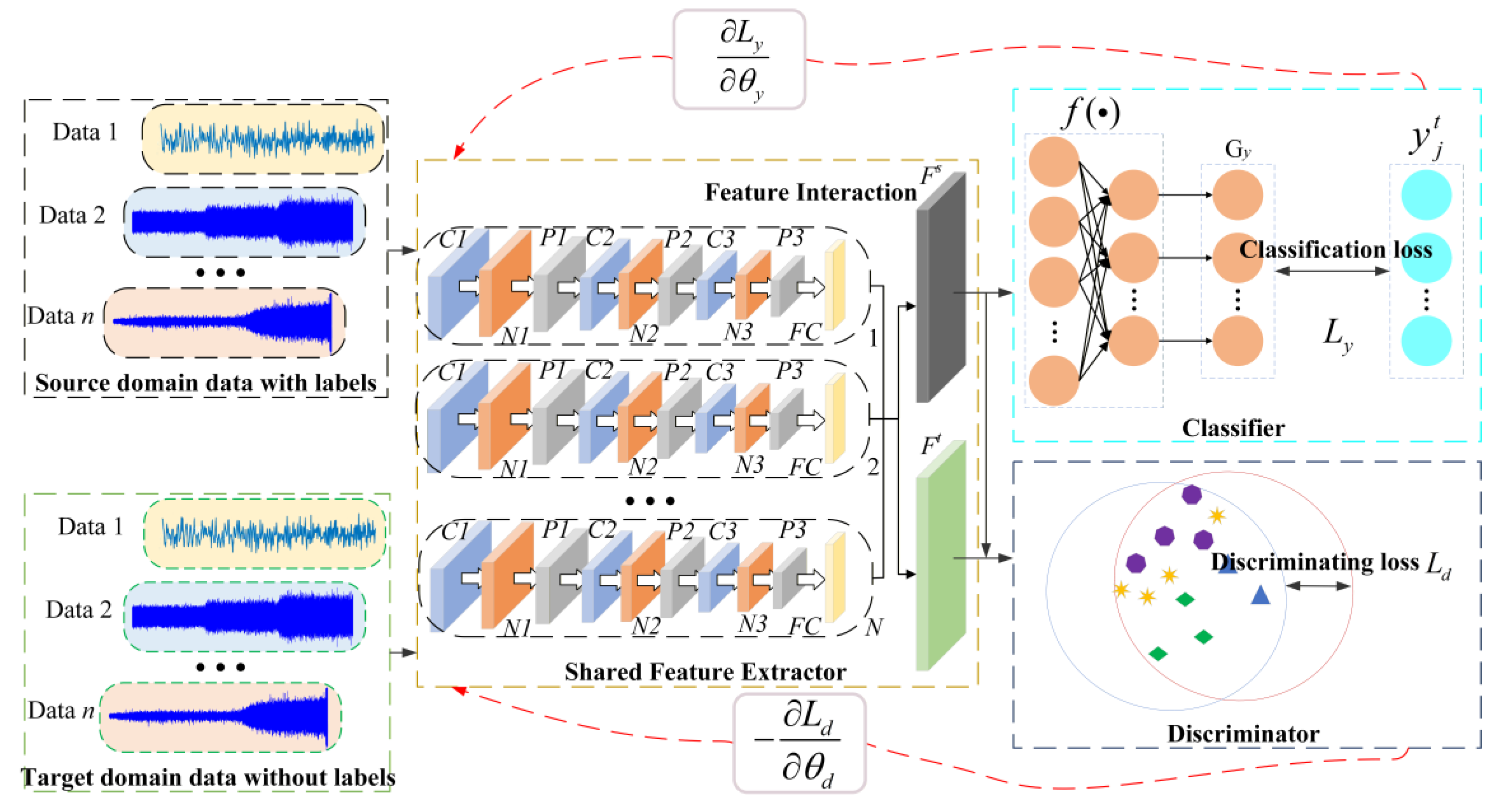
The proposed FI-DANN in this study is an improved version of the DANN model based on the model proposed by Ganin et al. [
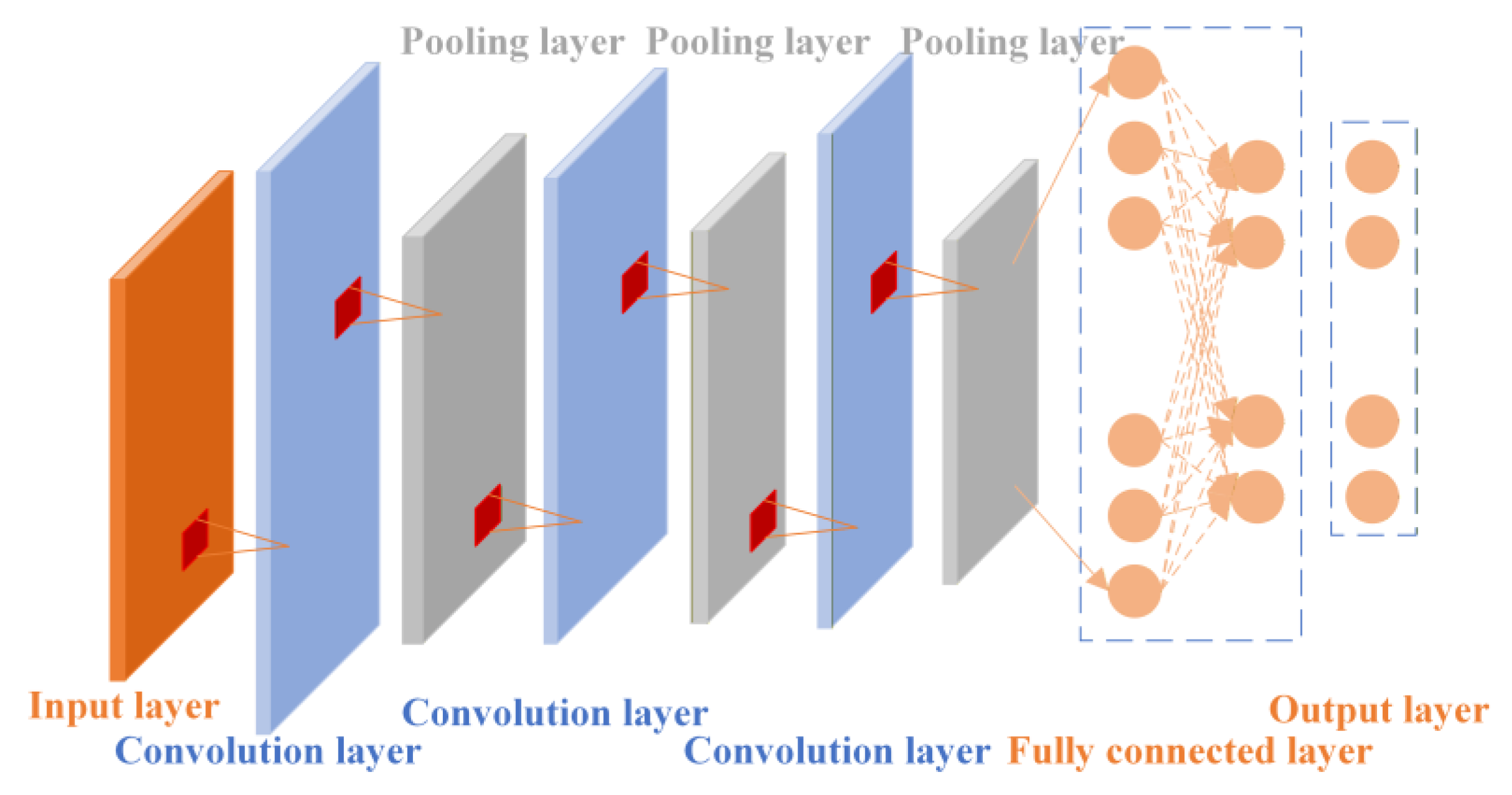
29]. It consists of three parts: a shared feature extractor, a classifier, and a discriminator. The shared feature extractor primarily performs feature extraction, interaction, and concatenation on data from both the source and target domains using multiple CNNs. The classifier is trained on data with labels in the source domain to ensure that the model possesses a high fault diagnosis capability. The discriminator achieves domain adaptation by progressively reducing the distribution discrepancy between the source and target domains, as shown in
Figure 3.
In
Figure 3,
and
represent three normalization layers are designed to eliminate dimensional differences among multi-source data;
is the convolutional layer, which is mainly responsible for performing convolution operations;
is the pooling layer, which is mainly responsible for reducing the number of parameters and computational complexity of the model through down-sampling.
is the fully connected layer, which integrates local features extracted from the convolution and pooling layers into a full feature through weighted summation. This result is then passed to the activation function to enhance the nonlinear expressive capability of the network.
represents the interacted features of the source domain data.
represents the interacted features of the target domain data.
is the label predictor.
is the classification loss.
is the discrimination loss.
3.2.2. Shared Feature Extractor
- (1)
Data pre-processing
To eliminate the dimensional differences between the multi-source data, the data input to the CNN was preprocessed.
where
represents the
data of the source domain or the target domain, and
and
represent the maximum and minimum values of the
dimensional data, respectively. Through the above processing, all dimensional data are standardized to the scale [0, 1].
- (2)
CNN Parameter Settings
To extract fault features from multi-source data,
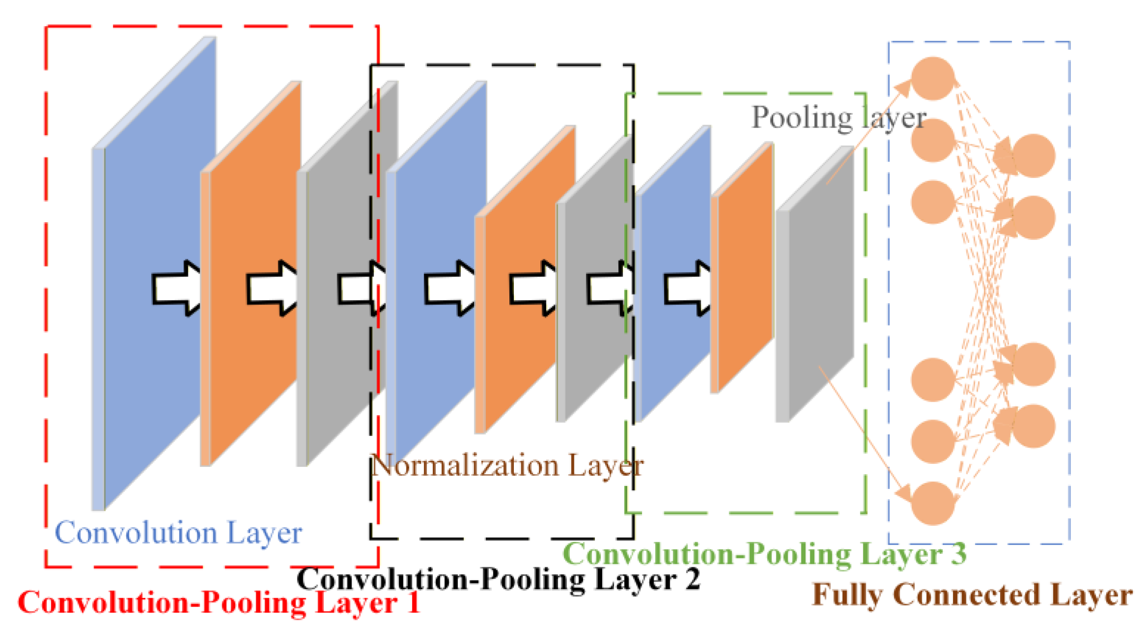
independent CNNs are set up for fault feature extraction, as shown in
Figure 4.
The shared feature extractor consisted of multiple independent CNNs, each containing three convolution-pooling layers and one fully connected layer. By employing convolutional kernels of varying sizes across these layers, the CNN effectively extracts both global and local features from time-series data based on different receptive fields. Simultaneously, to eliminate dimensionality differences among multi-source heterogeneous data and reduce feature distribution discrepancies across dimensionalities [
30,
31], normalization layers are inserted between each convolution-pooling layer in the CNN Structure.
- (3)
Feature Interaction
Compared to single-dimensional data, multi-source data can provide multi-faceted information on the fault features of aero-engines. Therefore, by selecting appropriate feature interaction methods to effectively interact with the fault features of multi-source data, we can not only more clearly represent the operating status information of aero-engines but also reduce the negative transfer when the source and target domains differ significantly or lack sufficient similarity. This enhances the accuracy, stability, and generalization capability of fault diagnosis models. Among the feature interaction methods, the Kronecker product [
32] is the most commonly used, with the following mathematical representation:
mutually independent CNNs are employed for fault feature extraction, yielding a total of source domain fault features and target domain fault features . Where and represent the source domain fault feature containing feature values and the target domain fault feature containing feature values, respectively.
Taking feature interaction in the source domain as an example, the formula for calculating the Kronecker product [
32] is as follows:
where
is the source domain interacted fault feature,
,
and
are the fault features extracted from the
i-th and
j-th dimensional data, respectively, and
and
are the
M-th dimensional fault features extracted from the
i-th and
j-th dimensional data via the CNN, respectively.
From the above formula, it can be seen that feature interaction can capture complex relationships among multi-source data, comprehensively considering the influence of multiple factors within the data. However, because it treats data from all dimensions as equally valuable, it is prone to negative transfer when fault features are selected inappropriately. When too many fault feature dimensions are selected, the resulting number of fault features by feature interaction becomes excessive, and the feature values tend to be small, making it difficult to extract key feature information. Information entropy is a measure of the information content within the data. When the entropy value is larger, it indicates that the data contains more information; when the entropy value is smaller, it indicates that the data contains less information. Therefore, to measure the fault information contained within each feature, this study combines information entropy with the Kronecker product to perform feature interaction.
Taking the source domain feature interaction as an example, the information entropy [
33,
34] of the source domain data is calculated.
where
is the information entropy of the
dimension. The dimension weight of the multi-source data is calculated.
where
is the weight of the
dimensional multi-source data,
. The Equation (6) can be updated as
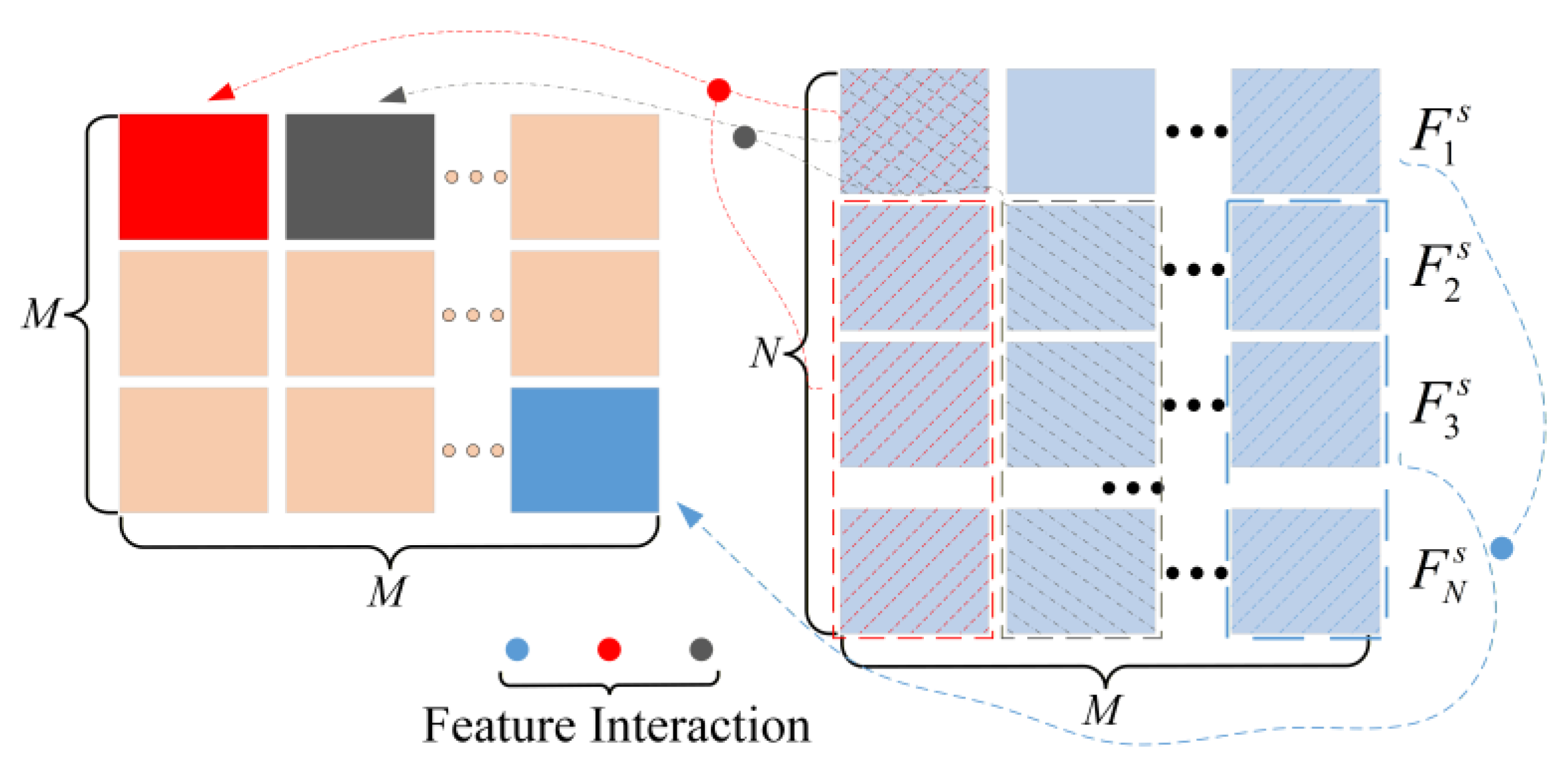
where
is the value in the interacted feature
, and its horizontal rows represent the interaction between the first-dimensional fault feature and fault features of other dimensions, as shown in
Figure 5.
By increasing the weight values constructed using information entropy, the proportion of fault features containing a large amount of information is effectively increased, whereas the proportion of fault features containing less information is effectively reduced. This enables the interactive features to represent various types of faults more accurately. Through adding logarithmic operations to the fault feature , the product operation () in Equation (6) is transformed into a linear operation, effectively preventing the possibility of dimensionality explosion when the dimensions of fault features become excessive. Through feature interaction, the interacted fault features can represent more fault information.
The calculation for the interacting fault features of the target domain follows the same procedure as above.
3.2.3. Discriminator [23,24]
To enhance the generalization capability of the proposed method in the target domain, it is necessary to evaluate the difference between the feature distributions of the source and target domains, thereby progressively decreasing the discrepancy through iteration. This study employs MMD to measure the difference between the interacted fault features
on the source domain and the interacted fault features
on the target domain. The formula is as follows:
While the proposed FI-DANN parameters are continuously updated, the value of the domain discrimination loss function will decrease progressively. The distance between the source and target domain feature distributions will also diminish progressively, thereby enhancing the generalization capability of the proposed FI-DANN.
3.2.4. Classifier [23,24]
Input the output activation value
of the source domain fault feature
and its corresponding label
into the classifier
to obtain the loss, which
is expressed as follows:
where
is the fault feature in the Formula (10), then the output
of the fully connected layer is
where
and
are the weights and biases of the fully connected layer, respectively, and
is the activation function.
The classifier employs Softmax, and a cross-entropy function is used to measure the loss. If the number of fault diagnosis labels is set to
, then the classification loss function
for the classifier is
where
is the total number of the source domain data, and
is the label of the source domain data.
Fault diagnosis using DANN leverages its domain-invariant property [
35], which reduces distribution discrepancies between the source and target domains. It is to minimize the classification loss function
and maximize the domain discrimination loss function
by solving for the parameters
in the shared feature extractor
. Where
and
represent the parameter sets in the classification loss function
and the domain discrimination loss function
, respectively.
Combining the domain discrimination loss function
and the classification loss function
, the total loss is
where
represents the adjustment factor, then aero-engine fault diagnosis can be regarded as an optimization problem.
The updating process of the fault diagnosis network parameters is as follows:
where
represents the learning rate, and all parameters are updated in each Epoch.
3.3. Training Process
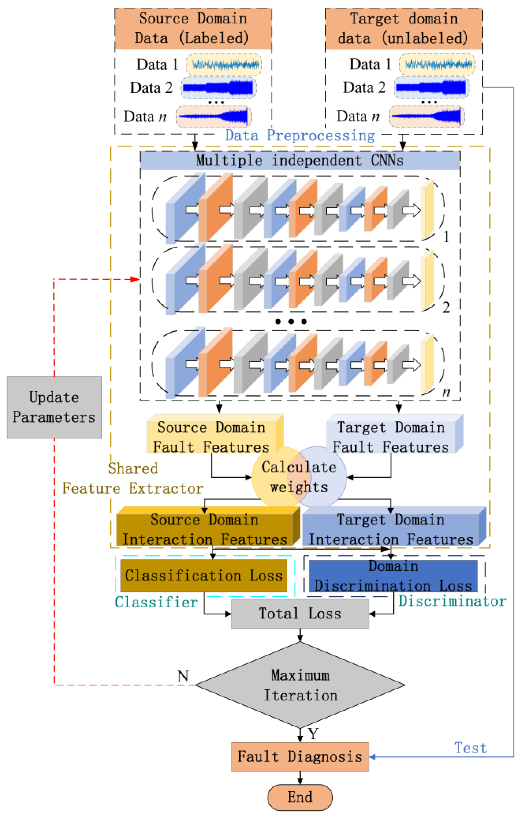
The training process for the FI-DANN is shown in
Figure 6.
Step 1: Collect multi-source data from various operating conditions of aero-engines, then perform preprocessing, classification, and standardization. Divide the data into training data (labeled data in the source domain, unlabeled data in the target domain) and test data (unlabeled test data in the target domain).
Step 2: Input the training data (divided into training and validation sets according to a proportion) into multiple independent CNNs for fault feature extraction.
Step 3: Combine the source domain features with the target domain features according to the dimensions and calculate the weights of each feature dimension using the information entropy.
Step 4: Employ the Kronecker product to perform feature interaction across dimensions, yielding source domain interacted features and target domain interacted features, respectively.
Step 5: Calculate the domain discrimination loss between the source domain interacted features and target domain interacted features using MMD. Employ Softmax to compute the probability of source domain features, and utilize the cross-entropy function to calculate the classification loss. Combine the domain discrimination loss function and classification loss function to construct the total loss function.
Step 6: Set the total loss function as the objective function. Utilize gradient descent to compute the classification loss and domain discrimination loss of the fault diagnosis, and update the network parameters through backpropagation.
Step 7: Repeat Steps 2–6 until the maximum iteration is reached.
Step 8: Input the test data into the trained FI-DANN to obtain fault diagnosis results.
4. Experiment Verification
4.1. Parameter Settings
In this paper, the CPU (i5-13400F) [Santa Clara, CA, USA] and graphics card (RTX 3060Ti) [Taipei, Taiwan, China] in the Anaconda environment with a deep learning framework PyTorch [2.4.0] were used for training the model.
Table 1 summarizes the model training parameters. The Adam optimizer was employed, with an initial learning rate of 0.001. The preprocessing time window is set to 1024, and the normalization option is set to 0–1 mode. The batch size is set to 256. The maximum number of iterations was set to 100. During the model training process, the learning rate was decayed by multiplying it by 0.1 at the 60th epoch.
According to
Section 3.2, the above can be represented as follows:
The source domain distribution set is , where , , , , and represent similar source domain distributions. that represent the typical fault in the source domain. Thus, the source domain dataset is . The data collected from the aero-engine requiring fault diagnosis follows the distribution , where is the number of target domain data, satisfying . This indicates a difference between the source domain distribution and the target domain distribution, that is, when , (where is the target domain label and ).
- (1)
Shared Fault Feature Extractor Settings
The parameter settings for multiple independent CNNs in the shared fault feature extractor are shown in
Table 2.
As shown in
Table 2, the CNN contains 3 convolution-pooling layers and 1 fully connected layer. The first convolution-pooling layer uses 32 convolutional kernels of size 1 × 3, the second layer uses 64 convolutional kernels of size 32 × 3, and the third layer uses 64 convolutional kernels of size 64 × 3. Each convolutional layer is activated using the ReLU function, and the parameter-controlled operation preserves the original values of the input tensor while returning a new tensor as output. The Dropout parameter in the fully connected layer (FC) is set to 0.5, which means 50% of the neurons are randomly ignored.
- (2)
Discriminator Settings
The discriminator selects MMD to measure the difference between the source Domain Interacted Fault Feature and the target Domain Interacted Fault Feature , then its discrimination loss is . Where MMD selects a single kernel, the kernel function selects a Gaussian kernel, and the bandwidth selects an adaptive bandwidth.
- (3)
Classifier Settings
The classifier employs the Softmax, and the cross-entropy function is selected to measure the classification loss .
The global optimization objective for the fault diagnosis is , and the hyperparameters for the fault diagnosis model are set as follows:
4.2. Case 1: Validation with Public Datasets
To validate generalization capability and stability, traditional CNN, DANN, and the FI-DANN proposed in this study were employed for fault diagnosis on bearing fault data from Case Western Reserve University in the United States. The experiment data in 2 dimensions were collected from accelerometers deployed at the drive end and fan end. The sampling frequency was 48,000 samples per second. The failure was set as a single-point electrical spark, located at the bearing inner diameter, with diameters of 0.007 inches, 0.014 inches, and 0.021 inches. The sampling rate was set to 10 samples per second, with a total sampling time of 11 min and 51 s.
Experiment setting: Source domain experimental parameters were set to a motor load of 3 horsepower and a rotational speed of 1730 rpm. Target domain experimental parameters were set to a motor load of 2 horsepower and a rotational speed of 1750 rpm, as shown in
Table 3.
For the experiments using traditional CNNs, source domain data and its corresponding labels are used as training data, with a training-to-validation ratio of 8:2, and target domain data and its corresponding labels are used as test data.
For experiments using traditional DANN, all experimental data were selected from the drive end. The training data included source domain data and 90% of the target domain data (data selection approach: extracted 90% from each of the four failure mode datasets in
Table 3). In the current experiment, the training-to-validation set ratio was 8:2, with the remaining 10% of target domain data serving as the test set.
For experiments conducted using the proposed FI-DANN, experimental data comprises both drive-end data and fan-end data. The training data includes source domain data and 90% of the target domain data (data selection approach: extracted 90% from each of the four failure mode datasets in
Table 3). In the current experiment, the training-to-validation set ratio was 8:2, with the remaining 10% of target domain data serving as the test set.
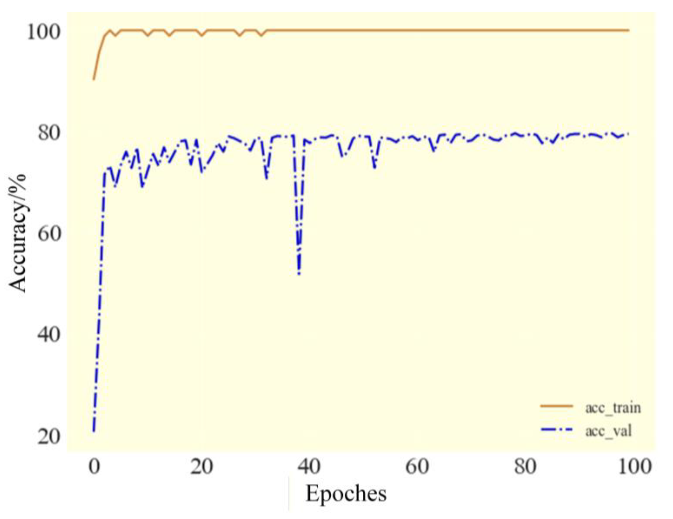
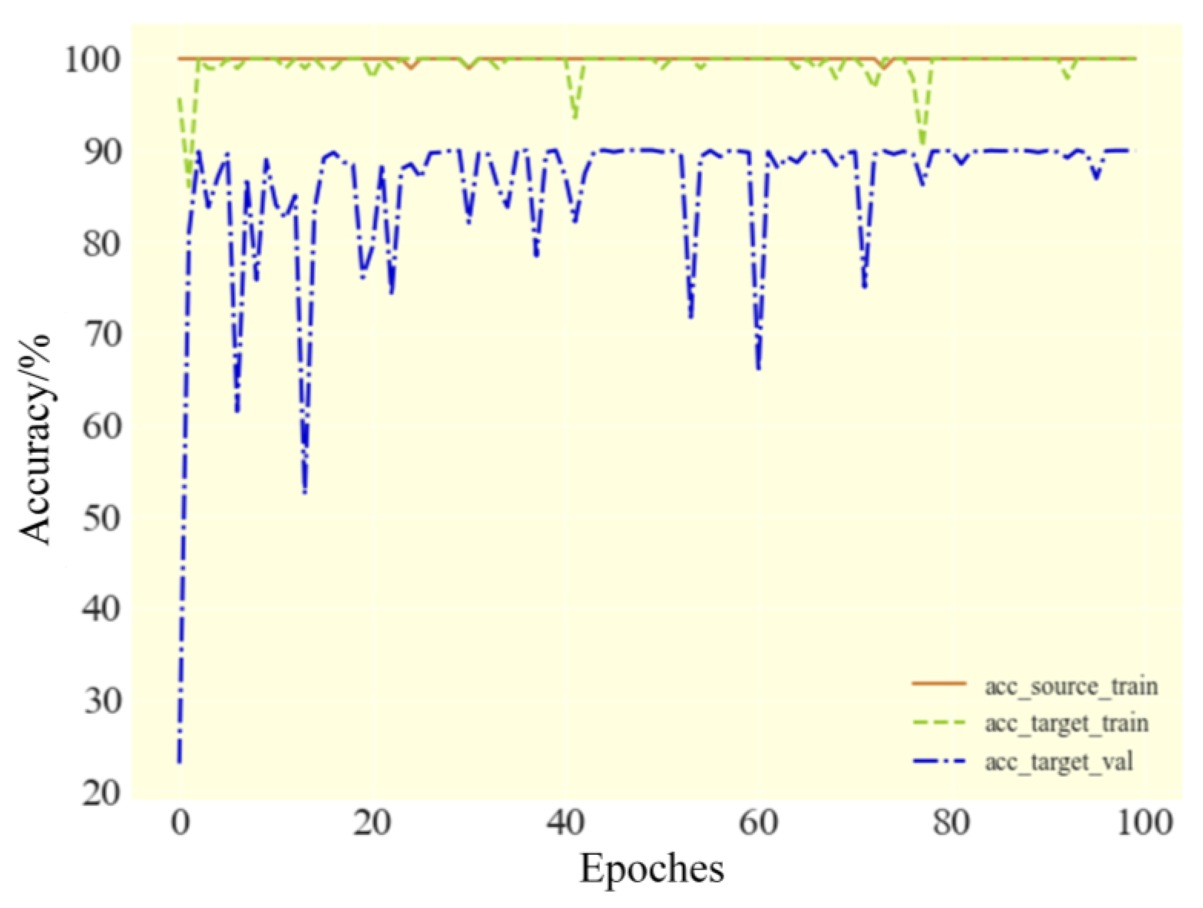
Each of the above experimental Data sets underwent 10 simulations, and the average values of its fault diagnosis accuracy were statistically calculated. The experimental results are shown in
Table 4 and
Figure 7,
Figure 8 and
Figure 9.
As shown in
Table 4 and
Figure 7, although the traditional CNN fault diagnosis algorithm reaches a high accuracy of 99.30% in the source domain, its test accuracy in the target domain only achieves 79.64%. This demonstrates that the traditional CNN fault diagnosis algorithm has weak generalization capabilities, resulting in low fault diagnosis efficiency in practical applications.
As shown in
Table 4 and
Figure 8, the validation accuracy of the traditional DANN fault diagnosis algorithm can reach 99.62%, but its test accuracy on the target domain can only reach 90.00%. Compared to traditional CNN algorithms, the traditional DANN fault diagnosis accuracy, although improved, the efficiency improvement is not significant, approximately 13.01%, and there is still considerable fluctuation after stabilization, with a standard variance is 0.06641. Since the number of experiments is 10, which is less than 30, the
t-distribution is used to calculate the confidence interval. At a 95% confidence level,
, and the confidence interval is [85.2%, 94.8%]. The fluctuation range is 9.6%. This demonstrates that although the traditional DANN fault diagnosis algorithm has enhanced its generalization capability, it still does not meet the requirements of practical applications.
As shown in
Table 4 and
Figure 9, the validation accuracy of the FI-DANN fault diagnosis algorithm can reach 99.81%; compared to the validation accuracy of the DANN algorithm (99.62%), the improvement is slight. However, its test accuracy can still reach 99.03%, compared to traditional CNN and traditional DANN fault diagnosis algorithms, the accuracy improvement is about 25.57% and 11.11%. Furthermore, the standard variance of accuracy after stabilization is 0.06258. Since the number of experiments is 10, which is less than 30, the
t-distribution is used to calculate the confidence interval. At a 95% confidence level,
, and the confidence interval is [94.6%, 100%]. The fluctuation range is 5.4%, which is smaller compared to the 9.6% fluctuation range of the traditional DANN algorithm’s confidence interval. This demonstrates that the FI-DANN fault diagnosis algorithm has high stability and significant practical applicability.
4.3. Case 2: Fault Diagnosis Using Multi-Source Data Collected from Aero-Engines
To demonstrate the generalization capability and feature interaction capability of the proposed FI-DANN fault diagnosis method, analysis data were collected from four engines of a type (No. 27, 28, 29, and 30) operated by China Eastern Airlines from 2017 to 2024. The data included metal concentration
in lubricating oil, lubricating oil pressure difference
, high-pressure rotor speed
, vibration value
, and lubricating oil temperature
. The engine sampling frequency is 10 samples/second. The sampling data volumes for engines 27 to 30 are 320,314, 222,335, 3,689,454, and 437,820, respectively. Same as Case1, the data preprocessing time window is 1024, and the normalization option is set to 0–1 mode. Four typical failure categories of this type of aero-engine since its service entry were selected: fan/compressor blade dysregulation, foreign object damage, transmission chain or accessory case component damage, and lubricating oil leakage. The simplified maintenance logs for aero-engines Nos. 27, 28, 29, and 30 are shown in
Table 5.
Four typical failure data of aero-engine No. 27, No. 28, and No. 30 are selected as the source domain data, while four typical failure data of aero-engine No. 29 are selected as the target domain data. The source domain data and 50% of the target domain data are used as training data, with a training-to-validation ratio of 8:2, and the target domain data and its corresponding labels are used as test data. This is to validate the generalization capability of the proposed FI-DANN fault diagnosis algorithm in practical applications, as shown in
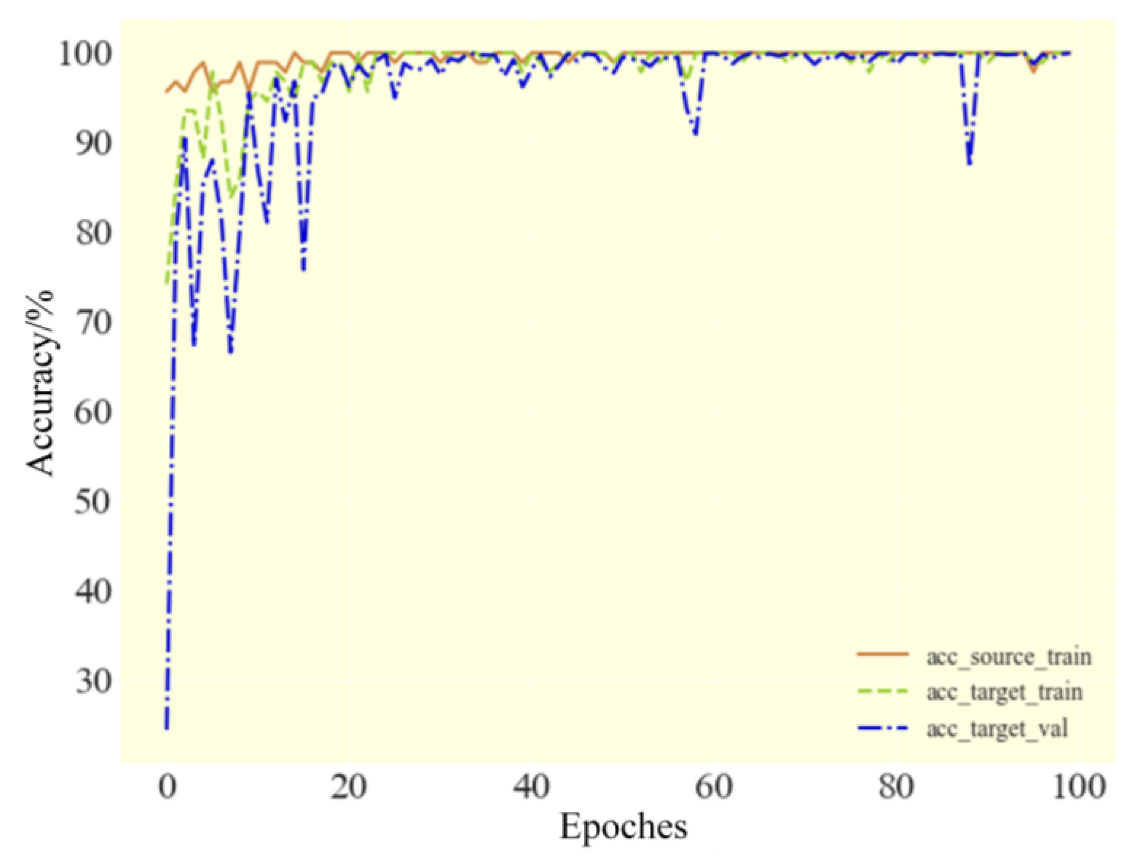
Figure 10.
As shown in
Figure 10, although the fault diagnosis accuracy of FI-DANN decreased compared to its performance on rolling bearings (99.03%), it still remained above 96%, which indicates that FI-DANN has a stronger generalization capability in the vertical dimension. Through
Table 6, it can be seen that the fault diagnosis accuracy of FI-DANN is significantly higher than that of CNN and DANN, which indicates that FI-DANN has a strong generalization capability in the horizontal dimension.
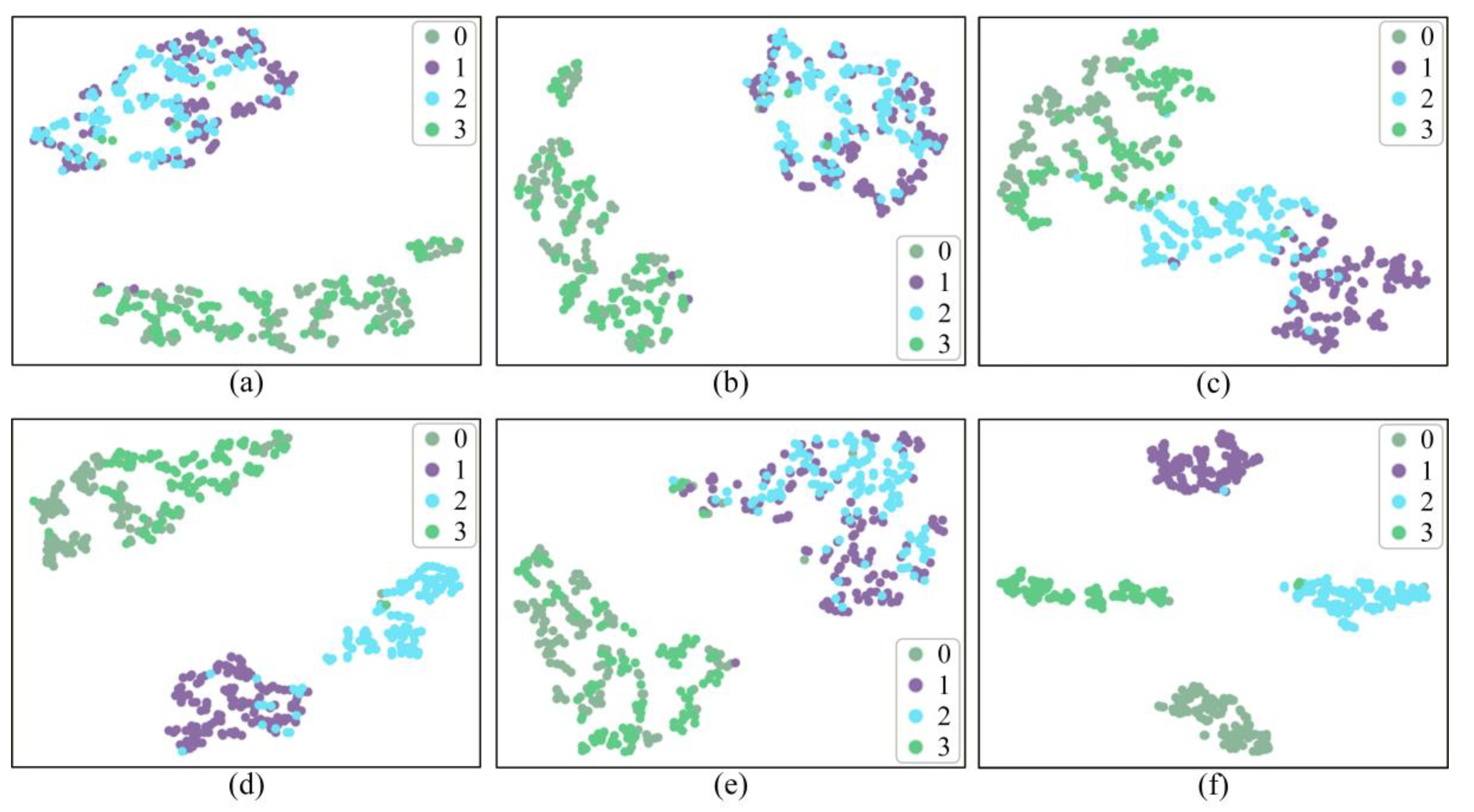
To further analyze the feature interaction effects of FI-DANN, the t-distributed stochastic neighborhood embedding (t-SNE) employed in References [
36,
37] was used to visualize the five types of source domain features and compare with the interacted features, as shown in
Figure 11.
Conversely, in
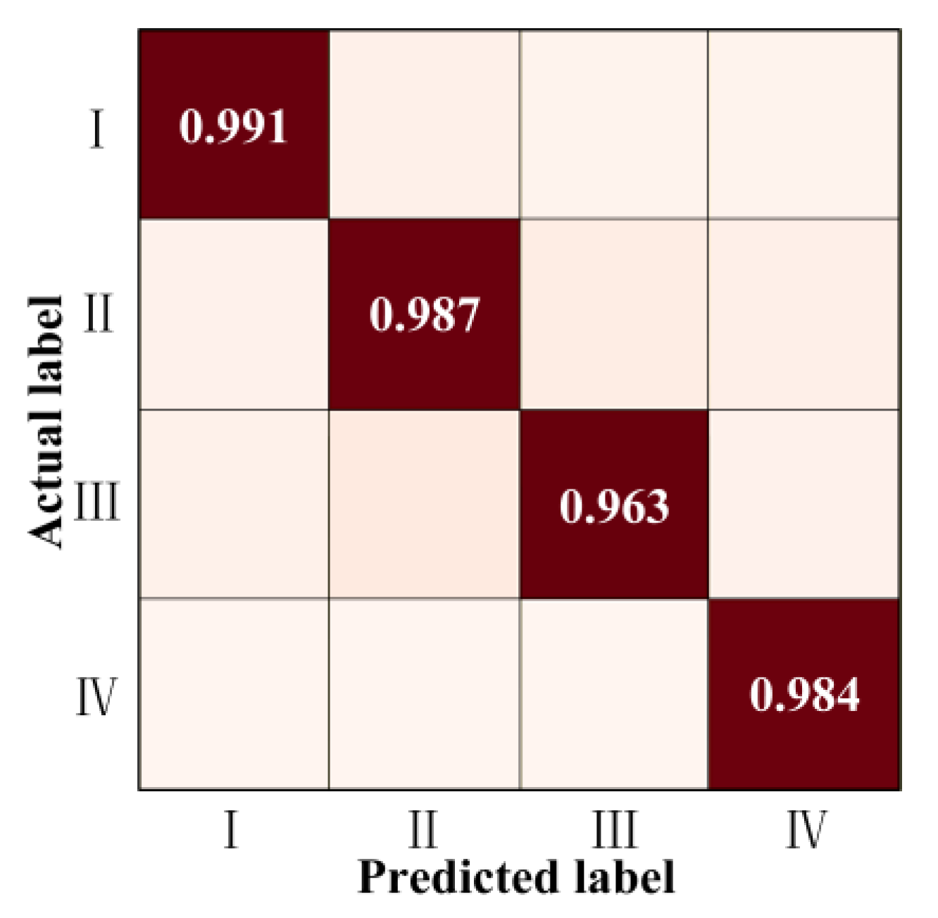
Figure 11f, the boundaries between the four typical fault features are distinctly clear, with highly concentrated features within each type and only a minimal number of misclassified features. The proposed FI-DANN achieves diagnostic accuracies of 99.1%, 98.7%, 96.3%, and 98.4% for the four typical failures, respectively. Therefore, the proposed FI-DANN can clarify the complex relationships among features across different dimensions and transfer the learned knowledge from the source domain to the target domain. It possesses high generalization capability and can efficiently identify various failures.
5. Conclusions
To address the issues of weak generalization capability and insufficient stability caused by significant differences in fault distribution between the source domain and target domain, this study proposes a FI-DANN. It was validated using public datasets and actual fault data from a type of aero-engine. Experimental results indicate the following:
- (1)
The method proposed by this study can effectively extract fault feature information from multi-source data, making the boundaries between different types of fault features more distinct and enabling clearer classification.
- (2)
Experimental results demonstrate that the method proposed in this study can overcome negative transfer caused by excessive distribution differences between the source domain and target domain. In case 1, it achieved a fault diagnosis accuracy of 99.03%, outperforming traditional models in both generalization capability and stability. In case 2, its fault diagnosis accuracy exceeded 96%, exhibiting strong generalization capabilities and practical application value.
However, this paper still has many unresolved issues, including availability in source domain labels, potential sensitivity to sensor selection or hyperparameters, and the lack of interpretability analysis for deep features. Future research should focus on developing a unified framework with strong robustness against hardware and parameter selection, while clarifying the underlying mechanisms of feature representation by incorporating explainable artificial intelligence methods. Concurrently, experimental designs must explicitly include sensor robustness testing and system interpretability verification, which is a key direction for advancing this field.