A Comprehensive Performance Evaluation of YOLO Series Algorithms in Automatic Inspection of Printed Circuit Boards

Abstract

Considering the rapid iteration of you-only-look-once (YOLO)-series algorithms, this paper aims to provide a data-driven performance spectrum and selection guide for the latest YOLO series algorithm (YOLOv8 to YOLOv13) in printed circuit board (PCB) automatic optical inspection (AOI) through systematic benchmarking. A comprehensive evaluation of the six state-of-the-art YOLO series algorithms is conducted on a standardized dataset containing six typical PCB defects: missing hole, mouse bite, open circuit, short circuit, spur, and spurious copper. An innovative dual-cycle comparative experiment (100 rounds and 500 rounds) is designed, and a systematic assessment is performed across multiple dimensions, including accuracy, efficiency, and inference speed. The experimental results have revealed significant variations in algorithm performance with training cycles: under short-term training (100 rounds), YOLOv13 achieves leading detection performance (mAP50 = 0.924, mAP50-95 = 0.484) with the fewest parameters (2.45 million); after full training (500 rounds), YOLOv10 achieves the highest overall accuracy (mAP50 = 0.946, mAP50-95 = 0.526); additionally, YOLOv11 shows the optimal speed-accuracy balance after long-term training, while YOLOv12 excels in short-term training; moreover, “open circuit” and “spur” are evaluated as the most challenging defect categories to detect. The findings given in this paper indicate the absence of a universally applicable “all-in-one” algorithm and propose a clear algorithm selection roadmap: YOLOv10 is recommended for offline analysis scenarios prioritizing extreme accuracy; YOLOv13 is the top choice for applications requiring rapid iteration with tight training time constraints; and YOLOv11 is the best option for high-throughput online inspection PCB production lines.

1. Introduction

As the core component of modern electronic devices, the quality and reliability of printed circuit boards (PCBs) directly determine the performance, lifespan, and stability of electronic products. With the rapid development of electronic technology towards high density, miniaturization, and multilayering, the wire spacing and pad size on PCBs have entered the micrometer level, which makes the production process prone to various defects such as missing hole, mouse bite, open circuit, short circuit, spur, and spurious copper. These defects may cause the entire PCB to malfunction, and even lead to the collapse of the entire electronic system [1,2,3,4,5]. Therefore, implementing efficient and accurate defect detection in the PCB manufacturing process is of great significance for improving product quality, controlling production costs, and enhancing the market competitiveness of enterprises.

During the past decade, the you-only-look-once (YOLO) series algorithms based on deep learning (DL) provides a revolutionary solution for high-speed and high-precision automated inspection and defect detection for PCBs, thanks to its single-stage defection framework and end-to-end training advantages [6,7,8,9,10]. However, the rapid iterative updates of the YOLO series algorithms have also brought new problems to industrial practice; current research lacks systematic comparative analysis of mainstream YOLO series algorithms on standardized PCB defect datasets, especially in terms of convergence performance under limited training cycles, and fails to clearly reveal the differences in sensitivity of different algorithms to various types of defects. This knowledge gap seriously hinders the correct selection and implementation of optimal algorithms in industrial practice. Therefore, this paper aims to fill the key gaps mentioned above through rigorous benchmarking, and provide a key algorithm selection guide and performance benchmark for the industry. The main contributions of this article are reflected in the following three aspects:

(1)

A dual-cycle benchmark testing framework for industrial decision-making has been built. For the first time, this paper empirically evaluates cutting-edge YOLO series algorithms from YOLOv8 to YOLOv13 on a unified standardized PCB defect dataset, and innovatively introduces a dual comparative experimental design with a limited training period (100 rounds) and complete training period (500 rounds). This framework not only evaluates the ultimate performance limit of the algorithm, but also simulates the actual needs of the industry in resource-constrained and rapidly deployable scenarios, accurately quantifying the trade-off between convergence speed and final accuracy of each algorithm, providing detailed insights for industrial algorithm selection.

(2)

The specificity sensitivity of different algorithms to defect types has been revealed. The evaluation exceeds the average accuracy of generalization, providing a comprehensive analysis from multiple dimensions such as average accuracy (mAP50, mAP50-95, and mAP75), precision, recall, parameter count, computational complexity, and inference speed. The research results clearly indicate that there is no single omnipotent algorithm: YOLOv10 has shown the highest comprehensive accuracy (94.6% mAP50) after long-term training, while YOLOv13 has shown excellent convergence and parameter efficiency in short-term training. More importantly, “open circuit” and “spur” have been quantitatively identified as the most difficult categories to realize defect detection across algorithm consistency, which points out a key direction for future research.

(3)

An algorithm roadmap for specific industrial application scenarios has been proposed. Based on detailed experimental data, this paper abandons empty theoretical discussions and instead proposes a highly operational decision guideline. It is strongly recommended via experiment that YOLOv10 should be preferred in offline analysis scenarios that pursue ultimate detection accuracy; YOLOv13 should be chosen in applications where training time is tight and rapid iterations are required; and YOLOv11 should be employed for high-throughput online detection production lines so as to provide optimal speed accuracy balance. This guideline based on strict benchmarking can provide a crucial practical basis and theoretical support for PCB manufacturing enterprises to efficiently and reliably integrate advanced DL models into their quality assurance systems, promoting the industrial application process of automated inspection for PCBs.

The rest of this paper is organized as follows: Section 2 provides a literature review on defect detection for both PCBs and YOLO series algorithms; Section 3 describes the specific experiment design for the comprehensive performance evaluation that is supposed to be performed in this paper, including the framework of the empirical evaluation, key indicators of the evaluation and their explanations, and the chosen specific YOLO series algorithms to be evaluated; after the data resource statement, Section 4 focuses on the aforementioned dual comparative experiment with a limited training period and complete training period for the YOLO series algorithm chosen, provides the experimental results of those key evaluation indicators for each algorithm, and carries out the detailed analysis of applicability of different algorithms under different PCB defect detection requirements; and Section 5 provides a conclusion of the entire paper.

2. Literature Review

2.1. Defect Detection for PCBs

In the early stages of detection technology development, PCB manufacturing companies generally relied on manual visual inspection. This method not only has high labor intensity and low detection efficiency, but is easily influenced by the subjective state of the detection personnel as well, resulting in high false detection and omission rates. Thus, it is difficult to meet the strict requirements of consistency and reliability in the modern manufacturing industry. To overcome the limitations of manual inspection, automatic optical inspection (AOI) technology has emerged and gradually become the mainstream of defect detection for PCBs [1]. AOI technology integrates optical imaging, precision machinery, and image processing techniques. It automatically captures PCB images through cameras and uses computer algorithms for defect analysis and recognition [2,3,4,5]. Traditional AOI systems typically use a reference comparison method, which compares the test PCB with a standard defect-free PCB. Furthermore, defect classification can be achieved by combining the background connected domain analysis method with a copper material detection method.

Although traditional AOI technology has significantly improved detection efficiency, it still has obvious limitations. Firstly, extremely high registration accuracy is required, and subtle registration errors may lead to a large number of false defect signals; secondly, feature extraction relies on manual design, and its generalization ability is insufficient for defect types with complex backgrounds and varied shapes; and furthermore, traditional algorithms typically have high computational complexity, making it difficult to meet the urgent demand for real-time detection in modern high-speed production lines. These limitations have collectively given rise to DL-based defect detection methods, especially the YOLO series algorithms, which have begun to emerge in the field of automatic inspection of PCBs [6,7,8,9,10].

2.2. YOLO Series Algorithms and Their Applications

YOLO is a revolutionary object detection paradigm first proposed by Redmon et al. [11]. Unlike traditional two-stage detection methods, YOLO reconstructs object detection as a single regression problem, directly mapping image pixels to bounding box coordinates and category probabilities. This pioneering idea lays a solid foundation for real-time object detection and propels a paradigm shift in the entire field of computer vision. The technological evolution path of this series of algorithms is shown in

Table 1. Review of YOLO series algorithms.

Specific Algorithms	Literature No.	Tasks Can Be Realized
		Object Detection	Classification	Multi Scale Detection	Target Tracking	Instance segmentation	Pose Estimation	Directional Object Detection
YOLOv1	[11]	√	√
YOLOv2	[12]	√	√
YOLOv3	[13]	√		√
YOLOv4	[14]	√			√
YOLOv5	[15]	√				√
YOLOv6	[16]	√				√
YOLOv7	[17]	√			√	√
YOLOv8	[18]	√				√	√
YOLOv9	[19]	√				√
YOLOv10	[20]	√
YOLOv11	[21]	√				√	√	√
YOLOv12	[22]	√
YOLOv13	[23]	√
YOLO26	[24]	√	√			√	√	√

“√” given in this table means that the corresponding task in that column can be realized by the corresponding algorithm in that row.

.

To be specific, YOLOv1 has pioneered a unified architecture. It has transformed object detection into a single regression problem; the convolutional neural network (CNN) used in it can directly predict bounding box and class probability through a single forward propagation, laying the foundation for real-time object detection [11]. YOLOv2 has introduced an anchor box mechanism; it has used a prior anchor box obtained through k-means clustering to improve bounding box prediction, and moreover, it has also realized multi-scale training; namely, it can adapt to different input sizes, improving robustness and detection ability for targets of different sizes [12]. YOLOv3 has built a more powerful backbone network with residual connections, effectively alleviating the gradient vanishing problem in deep networks; it has also realized multi scale prediction, by detecting three feature maps of different scales. Its detection performance of small targets has been significantly improved [13]. YOLOv4 has achieved the optimal balance between training efficiency and accuracy on the graph processing unit (GPU) by introducing the Mish activation function, and combining various advanced training techniques such as mosaic data augmentation [14]. YOLOv5 has provided a very user-friendly and modular implementation, greatly promoting its widespread use and deployment; it has also provided an anchor-box-free option, which provides an anchor-free detection head option, simplifying the design [15]. YOLOv6 has also used anchor-box-free design, which focuses on achieving extremely high deployment and inference efficiency in industrial production environments [16]. YOLOv7 has expanded the efficient layer aggregation network, and it has also used reparameterized convolution during its training phase to improve performance; moreover, it has performed architecture optimization to support more visual tasks such as tracking [17]. YOLOv8 has separated classification and regression tasks using decoupled detection heads, realized thoroughly anchor-box-free design, and further expanded support for tasks such as instance segmentation and pose estimation [18]. YOLOv9 has employed programmable gradient information (PGI) to solve the problem of information loss in deep networks and provide more complete gradient information for weight updates; it has further enhanced the feature learning ability and richness of the backbone network [19]. YOLOv10 has proposed a consistent dual allocation (CDA) strategy to eliminate the difference between training and inference by synergistically optimizing one-to-many and one-to-one label allocation; it has also introduced lightweight designs such as space channel decoupling downsampling and compact inverted block (CIB), which significantly reduce computational complexity while maintaining accuracy [20]. YOLOv11 has performed whole-process optimization, and extended the task to pose estimation and directional object detection [21]. YOLOv12 has introduced efficient region attention modules (low-complexity global self-attention) and residual blocks, pursuing Transformer-level model accuracy while maintaining the traditional high-speed advantage of YOLO series algorithms [22]. YOLOv13 has proposed an adaptive association enhancement and full process aggregation distribution scheme based on hypergraph to capture more complex feature interactions on a global scale [23]. YOLO26 has been designed for deep optimization of edge computing; it follows the three core principles of simplicity, deployment efficiency, and training innovation [24].

As YOLO series algorithms have outstanding performance in object detection and high-resolution image analysis, many industries are starting to use them in their critical production steps, including autonomous driving [25,26,27], remote sensing [28,29,30], smart agriculture [31,32,33,34,35,36,37], natural environment monitoring [38,39,40,41,42,43,44,45,46], medical image diagnosis [47,48,49], and PCB defect detection [8,9,10], as shown in

Table 2. Review of the industrial applications of YOLO series algorithms.

Specific Algorithms	Literature No.	Year Published	YOLO Series Algorithms Employed
			YOLOv8	YOLOv9	YOLOv10	YOLOv11	YOLOv12
Autonomous driving	[25]	2024	√
	[26]	2025	√
	[27]	2024	√
Remote sensing	[28]	2024	√
	[29]	2024		√
	[30]	2025	√
Smart agriculture	[31]	2025	√
	[32]	2024	√
	[33]	2024	√
	[34]	2025	√			√
	[35]	2025				√
	[36]	2025					√
	[37]	2024	√
Natural environment monitoring	[38]	2025	√
	[39]	2025	√
	[40]	2024	√
	[41]	2024	√
	[42]	2025		√
	[43]	2024	√
	[44]	2024	√
	[45]	2025			√
	[46]	2025	√
Medical image diagnosis	[47]	2025		√
	[48]	2025				√
	[49]	2025			√
PCB defect detection	[8]	2025			√
	[9]	2025					√
	[10]	2025					√

“√” given in this table means that the corresponding algorithm in that column has been employed in the research in that row.

.

It can be seen from Table 2 that the latest YOLO algorithms (say, YOLOv13 and YOLO26) have not been put into use immediately, and the algorithm with the highest application rate is YOLOv8. These interesting issues shown in the table also correspond to the focus of this paper, which aims to demonstrate through comprehensive performance evaluation what the characteristics of the latest algorithms in the YOLO series are, and which application scenarios they would be most suitable to be applied to.

2.3. Insights from Literature Review and Contribution of This Paper

The rapid trend of YOLO series algorithm iteration and the lack of systematic benchmark research pose substantial challenges to the high-reliability, real-time, and economical industrial field of PCB AOI, and have triggered multiple adverse consequences. The primary challenge lies in the algorithm selection dilemma faced by the industry and the decision costs associated with it. Due to the lack of clear performance benchmarks, PCB manufacturers lack robust algorithm selection criteria when deploying intelligent detection systems, and can only make empirical selection or time-consuming internal verification within those advanced YOLO series algorithms, which not only delays the intelligent upgrade cycle of the production line, but also directly increases the overall cost of technology integration and verification. The second challenge is the “sub-optimization risk” in technology deployment. Without a clear understanding of the convergence characteristics of YOLO series algorithms under limited training data, the sensitivity differences for different defect categories, and their unique trade-off between accuracy and inference speed, it is easy to encounter the problem of model capability not matching the requirements of real-world scenarios. In addition, the lack of recognized benchmarks also hinders the effective progression of research work. The lack of a consistent evaluation starting point in subsequent research makes it difficult to objectively quantify the improvement margin of new methods, thereby hindering efficient collaborative innovation between academia and industry around clear goals. Therefore, conducting a systematic performance evaluation of state-of-the-art YOLO series algorithms from YOLOv8 to YOLOv13 on a standard PCB defect dataset is of great significance.

The core objective of this paper is to provide an empirical data-based and actionable algorithm selection guide for the PCB AOI industry, in order to help it avoid decision risks, optimize deployment costs, and establish a clear performance benchmark to promote more targeted and comparable algorithm development. More specifically, in response to the lack of systematic horizontal comparisons of YOLO series algorithms from YOLOv8 to YOLOv13, and the widespread neglect of the crucial trade-off between convergence efficiency and overall performance in industrial scenarios, this paper has conducted a rigorous empirical study. A dual-cycle training paradigm (100 rounds and 500 rounds) and multidimensional evaluation system have been conducted for the first time on a unified PCB defect benchmark dataset, aiming to systematically reveal the differences in the short-term convergence and long-term performance of various algorithms. Ultimately, the goal of this paper is to provide the PCB AOI industry with a data-driven YOLO algorithm selection roadmap for different scenarios, in order to promote the efficiency and reliability of its intelligent defect detection technology.

3. Experiment Design

3.1. Algorithms Chosen for Empirical Evaluation

In terms of algorithm selection, this article chooses the latest versions of YOLO series algorithms, from YOLOv8 to YOLOv13, to perform the empirical performance evaluation for PCB defect detection. The choice of these algorithms is mainly based on the following considerations: (1) Although early versions from YOLOv1 to YOLOv7 have made pioneering contributions in the field of object detection, their feature extraction networks, multi-scale fusion mechanisms, and loss function designs have significant limitations compared to the new ones that have been chosen, especially when dealing with industrial detection scenarios such as small defects and complex backgrounds; they no longer have a competitive advantage in balancing accuracy and efficiency. (2) Although YOLO26 is the latest algorithm, it has not been officially released yet, and there is no source code to support research. (3) Algorithms from YOLOv8 to YOLOv13 not only inherit the advantages of previous ones in the series, but also achieve breakthrough innovations in neural network (NN) architecture, training strategies, and the loss functions mentioned in Section 2.1, making them more suitable for the detection requirements of small defects in industrial quality inspection, thus providing a more advanced and effective solution for PCB automated inspection.

3.2. Framework Design of the Experiment

The experiment designed in this paper tries to construct a systematic empirical research framework and establish a scientific algorithm selection benchmark by multidimensional evaluation of the performance of the six YOLO series algorithms chosen on a standardized PCB defect dataset. The experimental design strictly follows the principle of controlling variables: firstly, constructing a standardized dataset containing six typical defects: missing hole, mouse bite, open circuit, short circuit, spur, and spurious copper, which are explained in detail in

Table 3. Classification and characteristics comparison of common defects in PCB.

Defect Name	Formation Mechanism	Functional Hazards	Inspection Challenge
Missing hole	It is a serious abnormality in the drilling process, which means complete loss of through holes/boreholes due to incorrect paths, mechanical failures, or drill bit damage.	Lose vertical interconnection function, cause electrical open circuits between circuit layers, prevent power, ground, or signal transmission, and result in complete failure of the entire PCB or specific modules. It is a catastrophic process failure.	(1) Small object detection: Holes account for a very small proportion in the entire image. (2) Negative sample detection: It is necessary to identify objects that should exist but do not actually exist. (3) Distinguishing from imaging artifacts: Visual “holes” caused by lighting, shadows, etc., need to be excluded.
Mouse bite	It is an abnormal etching process. Due to mask defects, improper exposure, or uneven etching solution, the edges of the circuit are abnormally corroded, forming irregular serrated/wavy contours.	Reduce the cross-sectional area of wires, easily cause local overheating, accelerate aging or melting (open circuit), affect high-frequency performance, exacerbate skin effect, and reduce mechanical strength.	(1) Fine feature extraction: It is necessary to capture sub-pixel-level contour distortions. (2) Morphological complexity: Defects have irregular shapes and no fixed patterns. (3) High difficulty in defining: It is necessary to accurately distinguish between defects and allowable process fluctuations.
Open circuit	The continuous wires in the design are physically disconnected. It is mainly due to excessive etching, mechanical scratching, electric migration forming voids, or substrate crack propagation.	Interrupt signal or power path, and cause complete loss of downstream circuit functionality. It is one of the most fundamental and harmful defects.	(1) Multi scale perception: The size of the disconnect gap varies. (2) Connectivity analysis: It is necessary to understand the route direction at the semantic level and determine its continuity. (3) Background interference: The fracture may be located in a dense wiring area, which is easily concealed.
Short circuit	Unexpectedly connected wires that should have been insulated. It is mainly due to incomplete etching resulting in copper foil residue, or improper ink coverage of the isolation gap during the production of the solder mask layer.	Cause signal crosstalk and logic errors, and generate high current paths, which may cause component burnout due to overcurrent and even trigger fires, with great destructive power.	(1) Inspection of slender structures: Bridge copper wires are often small linear or mesh-like. (2) Low contrast issue: Residual thin copper foil may result in extremely low contrast between the defect area and the background. (3) Gap measurement accuracy: It is necessary to accurately measure the distance between the lines and determine whether it is below the safety standard.
Spur	After etching, isolated small copper particles or copper spikes (often referred to as copper slag) remain on the surface of the PCB or in the isolation groove and are not required by the design. It is mainly due to poor etching solution flushing or poor copper foil quality.	Have potential short circuit risk, displace and bridge critical circuits due to external influences, disrupt signal integrity, act as a miniature antenna in high-frequency circuits, and radiate or receive interference.	(1) Random detection of small targets: Micro sized particles with irregular shape and position. (2) High false positive rate: Easily confused with image noise, dust, scratches, etc. (3) Weak feature saliency: Isolated existence, lacking contextual information for judgment.
Spurious copper	A larger and irregularly shaped redundant copper foil area. It is usually due to damage or contamination of the photomask, large areas of copper foil that should have been etched away are not completely removed.	Have bridge risk, cause a short circuit in isolated circuit areas, have an impact on circuit performance such as changing local characteristic impedance, and pose a serious threat to high-speed digital and RF circuits.	(1) Irregular shape segmentation: The forms vary greatly and there is no fixed paradigm. (2) High segmentation accuracy requirements: Accurate pixel-level segmentation is required for areas with copper impurities. (3) Distinguish from legal copper areas: It is necessary to avoid mistaking design features such as tears and copper coating as defects.

; then, under a unified software and hardware environment, each algorithm is trained for 100 rounds (simulating limited training resources) and 500 rounds (a complete training cycle), respectively; and finally, quantitative evaluation was conducted from multiple indicators including average accuracy (mAP50, mAP50-95, and mAP75), precision, recall, parameter count, parameter count, computational complexity, and inference speed, which are explained in detail in

Table 4. Core indicators for quantitative evaluation of the YOLO series algorithms chosen.

Names of the Evaluation Indicators	Principle	Function
mAP50	The average accuracy mean of all categories under relaxed positioning requirements (if the overlap area between the predicted box and the real box exceeds 50%, it is considered correct)	Provide basic performance benchmarks. Reflect the comprehensive detection capability of the algorithm under conventional positioning accuracy requirements.
mAP75	The average accuracy mean for all categories under strict positioning requirements (if the overlap area between the predicted box and the real box exceeds 75%, it is considered correct)	Evaluate the positioning precision of the algorithm. The higher the value, the more accurate the position and size of the predicted box are.
mAP50-95	Change the intersection over union (IoU) threshold from 0.5 to 0.95 with a step size of 0.05, calculate mAP at multiple different strictness levels, and then take the average.	Provide the most comprehensive and rigorous performance evaluation. It is the golden indicator for measuring the comprehensive performance of an algorithm.
P (precision)	The proportion of true targets among all the “targets” predicted by the algorithm. It pays attention to the accuracy of the predicted results.	Evaluate the level of “false detections” in the algorithm. The higher the value, the more reliable the algorithm is, and the fewer false alarms.
R (recall)	The proportion of all real targets successfully detected by the algorithm. It pays attention to the ability of the algorithm to discover all targets.	Evaluate the level of “missed detections” in the algorithm. The higher the value, the more comprehensive the coverage.
M (parameter count, in millions)	The total number of weights and biases that need to be learned in the algorithm. It represents the scale and capacity of the algorithm.	Indirectly measure the complexity and memory usage of the algorithm. Algorithms with a large number of parameters have high potential, but deployment requires more storage space.
GFLOPs (computational complexity)	The number of floating-point operations required for an algorithm to complete one forward inference, measured in billions of times. It represents the computational complexity of the algorithm.	Evaluate the inference speed potential and hardware requirements of the algorithm. The lower the value, the faster the inference speed and the easier it is to deploy at the edge.
inference (inference speed)	The actual time required for the algorithm to process a single input image (or a batch) on specific hardware.	Directly measure the actual operational efficiency of the algorithm.

.

The results of 100 rounds of training can serve as an efficient pre-screening indicator for the convergence speed and potential of a certain algorithm, while the results of 500 rounds of training provide a reliable basis for the stable evaluation and ranking of the final performance of a certain algorithm. The two experiments can jointly reveal the differences in learning efficiency and ultimate performance of a certain algorithm, providing a comprehensive theoretical basis and practical guidance for algorithm selection for different application scenarios such as rapid prototyping verification and high-precision deployment.

4. Experiment Results and Analysis

4.1. Data Acquisition and Experiment Environment Setup

In this paper, PKU-Market-PCB dataset released by Peking University Intelligent Robot Open Laboratory (the link is given in the Section “Data Availability Statement”) is used to perform empirical evaluation for the YOLO series algorithms chosen. The dataset is designed specifically for PCB defect detection algorithm evaluation, and it contains 1386 high-resolution PCB images obtained from the actual manufacturing process, covering the six typical defects mentioned in Section 3.2. The dataset has been finely annotated with real labels to ensure the accuracy of model training and evaluation. The distribution of the samples of the six typical defects is shown in

Table 5. Distribution of the sample size of six typical defects.

Defect Class	Title 2	Percentage
Missing hole	230	16.6%
Mouse bite	230	16.6%
Open circuit	232	16.7%
Short circuit	232	16.7%
Spur	230	16.6%
Spurious copper	232	16.7%
Total	1386	100%

. It can be seen that the dataset exhibits a carefully designed high balance in the number of instances of the six typical defects. This balance effectively avoids the overfitting or underfitting of certain defects due to data distribution bias, providing an ideal foundation for a fair and comprehensive evaluation and comparison of the defect detection capabilities of different YOLO series algorithms.

The PKU-Market-PCB dataset exhibits strong industrial relevance in the following aspects:

(1)

Authenticity of data sources: The images in this dataset were collected from real PCB production lines and scrapped boards, and defects were confirmed and labeled by process engineers to ensure the authenticity of their morphology. The physical forms corresponding to the six typical defects included in it (such as abnormal holes, conductor gaps, spur, spurious copper, etc.) have targeted visual acceptance condition judgment diagrams in the authoritative industry-standard IPC-A-600K with the title “Acceptability of Printed Boards” [50]. Therefore, this dataset is suitable for appearance acceptance research based on IPC standards. IPC-A-600K is the latest version of the standard released by IPC in July 2020. It specifies the observable targets, specifies the acceptable and non-compliant conditions of printed circuit boards (bare boards) without assembled components in both internal and external aspects through detailed illustrations, and is an authoritative acceptance guide widely used in the industry.

(2)

Authenticity of imaging conditions: The images are collected in a controlled industrial optical inspection system environment, with uniform and stable photo contrast; this precisely simulates the internal imaging conditions of professional AOI equipment. Actually, the industrial AOI system just pursues a stable and controllable imaging environment through built-in light sources and enclosed structures, in order to minimize external light interference.

In summary, the PKU-Market-PCB dataset provides a comprehensive, reliable, and industry-relevant benchmark platform for systematically comparing and evaluating the core detection performance of YOLO series algorithms, based on real defect samples, typical defects, complex scenes with small target challenges, and the simulation of standard AOI imaging environments.

The training set and validation set are divided in a 7:3 ratio. The experimental hardware system in this paper adopts a high-performance computing platform, equipped with an Intel 13th generation i9-13900KF processor (with a main frequency of 3.00 GHz), 64 GB DDR4 memory, and an NVIDIA GeForce RTX 4080 SUPER graphics card (16 GB GDDR6X video memory), combined with a 3.68 TB NVMe solid-state storage system, providing sufficient parallel computing power and data throughput bandwidth for deep neural network (DNN) training and inference. The YOLO series algorithms used in this paper are based on their official or recognized mainstream open-source implementations, and adopt uniform hyperparameter settings. The algorithm code libraries, version numbers, and key hyperparameter settings are shown in

Table 6. Algorithm code library and version number of each YOLO series algorithm.

Specific Algorithms	Official Code Libraries in GitHub 1	Release Tag
YOLOv8	ultralytics/ultralytics	V8.3.176
YOLOv9	WongKinYiu/yolov9	V0.1
YOLOv10	THU-MIG/yolov10	V1.1
YOLOv11	ultralytics/ultralytics	V8.3.176
YOLOv12	sunsmarterjie/yolov12	V1.0
YOLOv13	iMoonLab/yolov13	yolov13

¹ GitHub is a leading global code hosting and collaborative development platform, providing code storage, version management, team collaboration, and open source community services.

and

Table 7. Key hyperparameter settings.

Hyperparameters	Full Name	Values
epochs	Training rounds	100 or 500
batch	Batch size	32
imgsz	Input size	640
optimizer	Optimizer	Adaptive moment estimation (ADAM)
close_mosaic	The number of cycles for mosaic enhancement has been turned off	10 or 20
lr0	Initial learning rate	0.01
lrf	Final learning rate factor	0.01
momentum	Momentum	0.937
weight_decay	Weight decay	0.0005

.

During the actual experiment to evaluate the YOLO series algorithms chosen, the core evaluation indicators mentioned in Table 4 are used for the final evaluation of those algorithms. Additionally, during the experiment, some training analysis indicators are also used for monitoring the training process of the YOLO series algorithms chosen; the training analysis indicators can be found in

Table 8. Training analysis indicators for monitoring the training process of the YOLO series algorithms chosen.

Names of the Evaluation Indicators	Principle	Function
train/box_loss (Training set bounding box regression loss)	Calculated during the forward propagation process of algorithm training, specifically to supervise and quantify the accuracy of the algorithm in predicting the spatial position and range of objects on the training set samples. Its core is to measure the geometric differences between the predicted bounding box and the real annotated box.	The decreasing trajectory of this loss value directly reflects the ability of the algorithm to learn the geometric distribution of objects from the training data. It is a key driving signal for optimizing algorithm parameters and mastering basic positioning capabilities. Continuous decline and convergence are the primary indicators of an effective training process.
train/cls_loss (Training set classification loss)	Calculated during the forward propagation process of algorithm training, specifically to supervise and quantify the accuracy of the classification of detected objects in the training set samples.	The optimization process of this loss value directly drives the algorithm to learn discriminative semantic features that distinguish different object categories. Its convergence trend reflects the establishment and consolidation of the classification and recognition ability of the algorithm.
train/dfl_loss (Training set distribution focusing loss)	Used in YOLOv8 and subsequent versions and calculated during the training phase. It represents an advanced bounding box regression paradigm, whose core is not to directly regress the determined values of boundary coordinates, but to guide the algorithm to predict a discrete probability distribution of coordinate values.	This indicator reflects the modeling ability and regression robustness for fuzzy object boundaries. Its effective reduction is the inherent mechanism for achieving sub-pixel-level high-precision positioning in the algorithm, representing an important innovation in the positioning accuracy of modern object detection algorithms.
val/box_loss (Verification set bounding box regression loss)	Calculated during the evaluation phase of algorithm training, specifically measuring the accuracy of the algorithm in predicting the spatial position and range of objects on independent validation set samples.	This indicator is the core criterion for evaluating the generalization of the localization ability of a certain algorithm. If its numerical stability is lower than or close to the training bounding box loss, it means that the algorithm has learned universal localization rules; if it is significantly higher than the training value, it suggests that the algorithm may have overfitting to the training data, and its localization ability cannot be transferred to the new scene.
val/cls_loss (Verification set classification loss)	Calculated during the evaluation phase of algorithm training, specifically measuring the discrimination accuracy of the algorithm for object categories in independent validation set samples.	This indicator is the gold standard for testing the algorithm’s generalization ability of semantic recognition. An algorithm with strong generalization ability should demonstrate an excellent level on this metric that is similar to the training classification loss. It is a key forward-looking indicator for predicting whether the algorithm can reliably identify various objects in actual deployment.

.

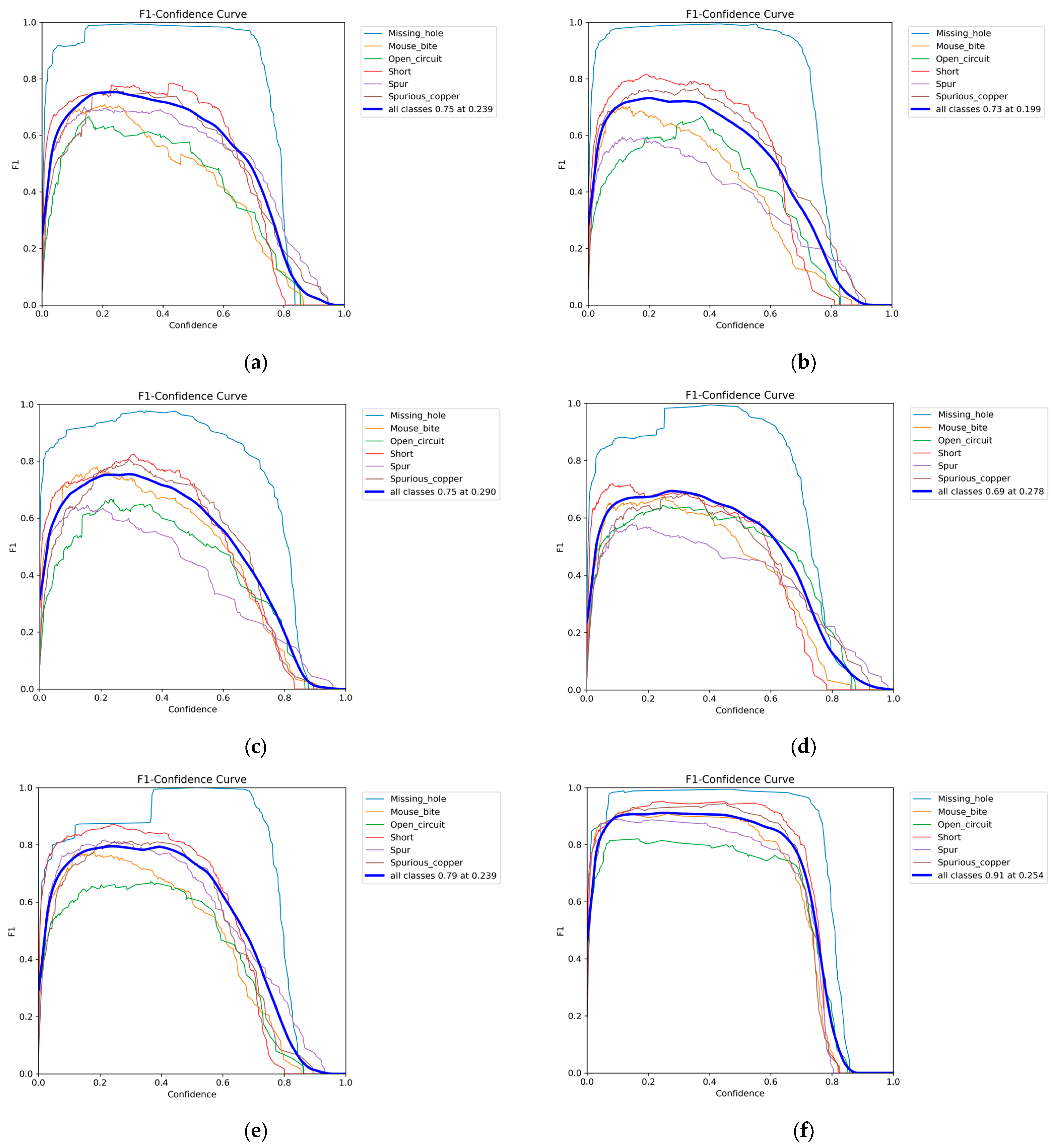
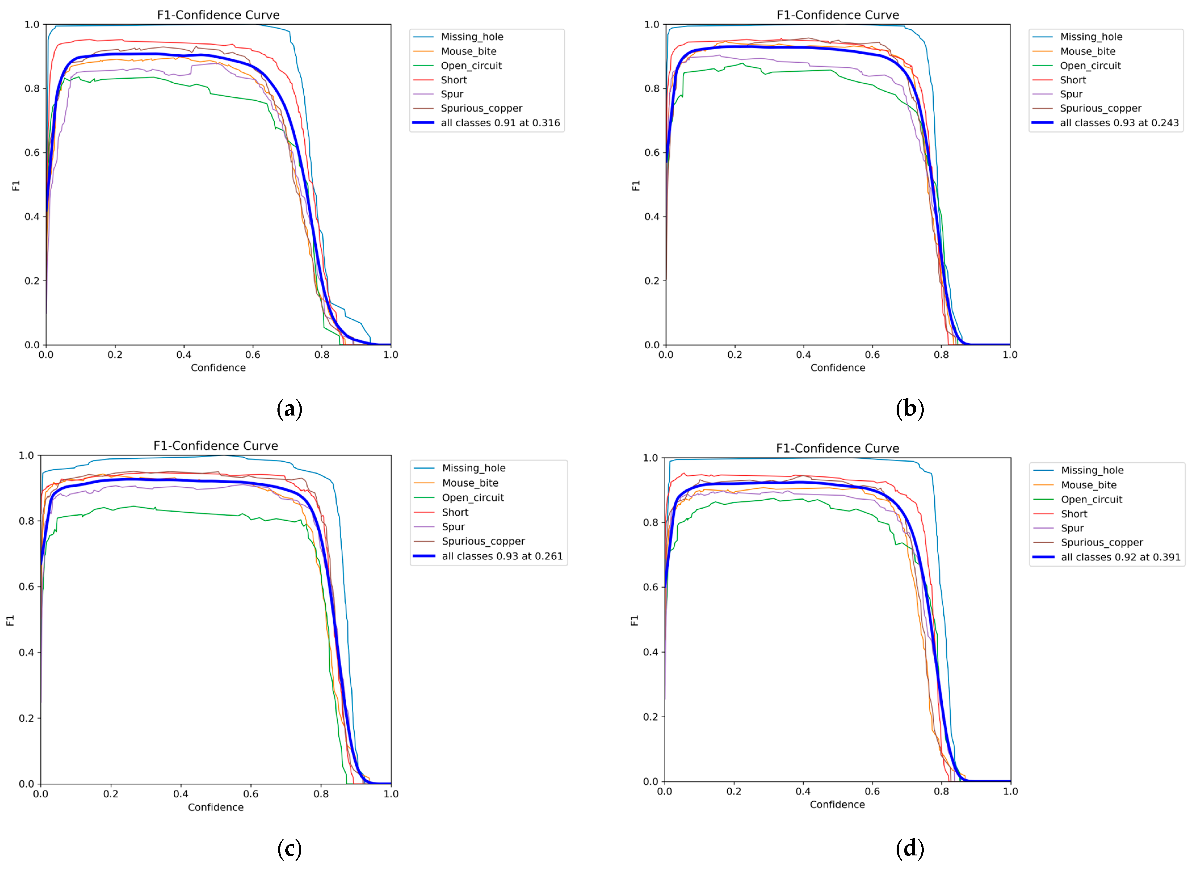
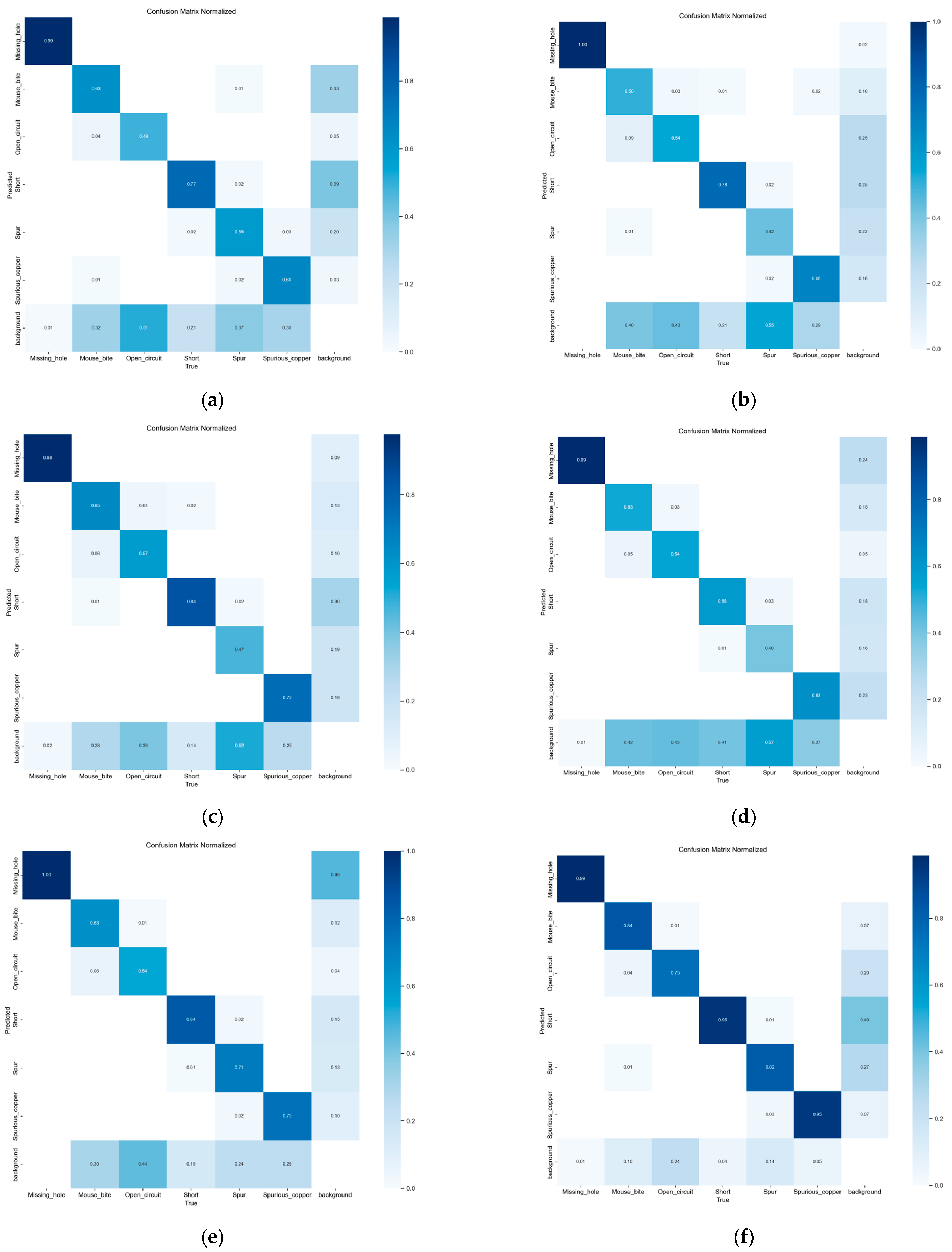
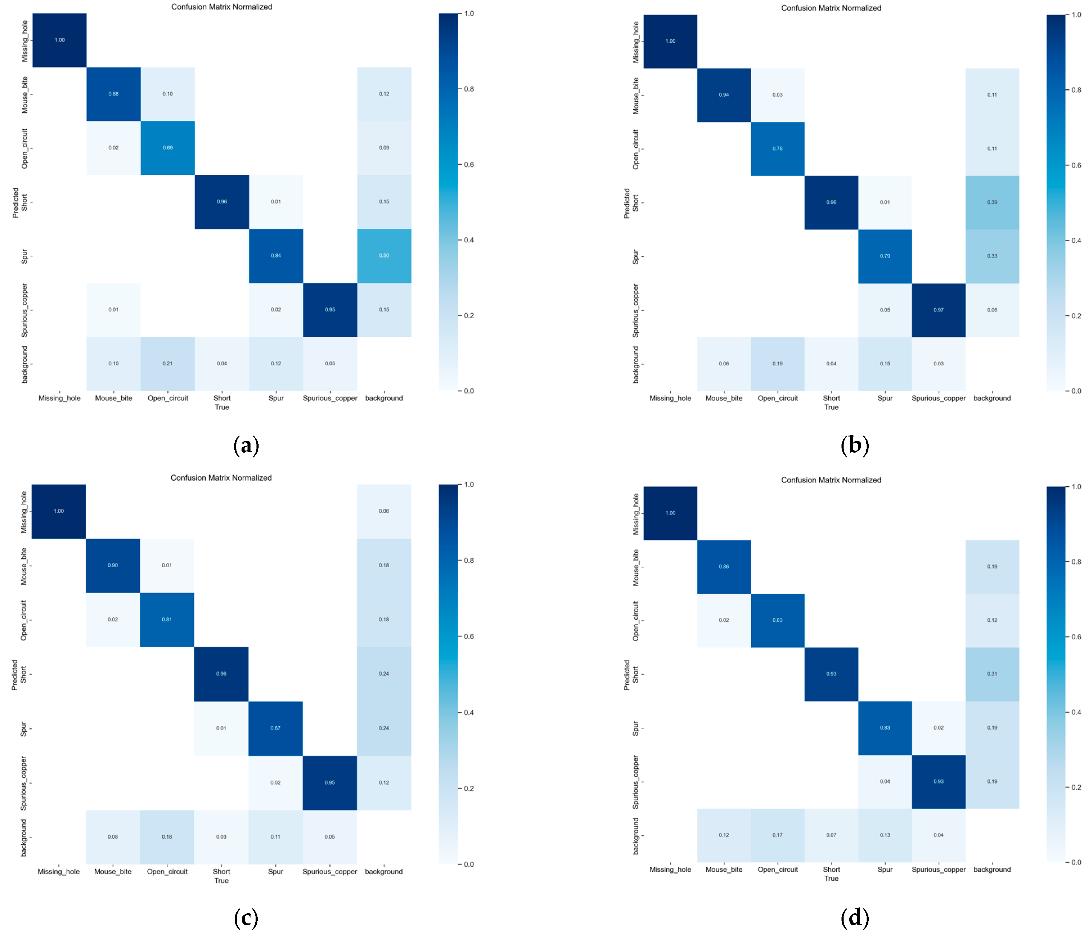
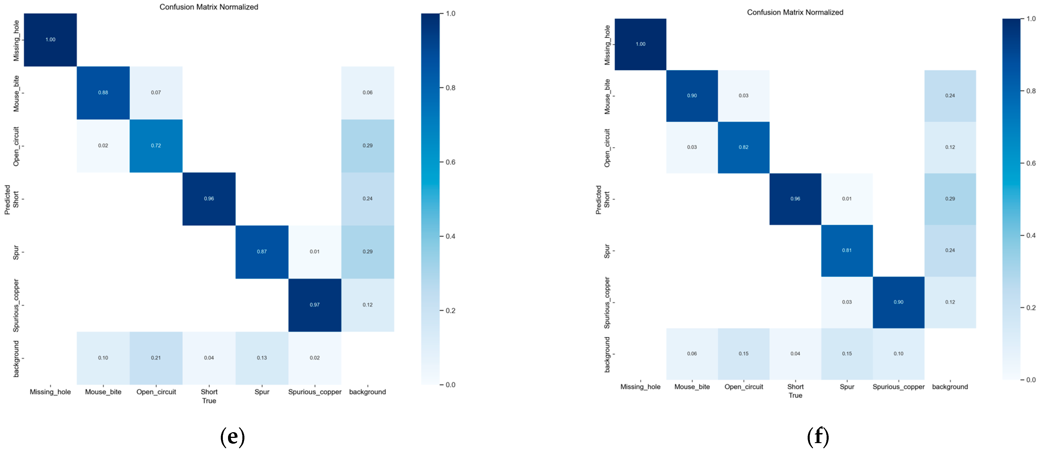
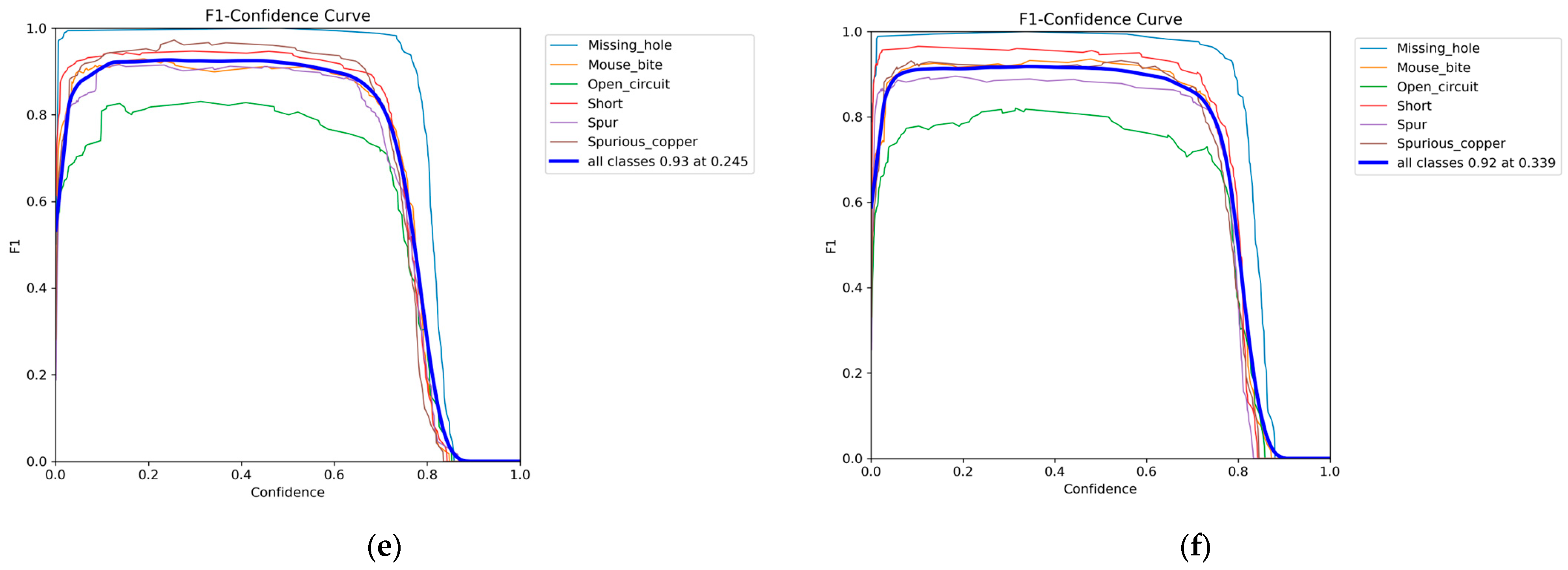
Apart from the indicators, a normalized confusion matrix and F1 confidence curve are also employed to evaluate the performance of the YOLO series algorithms chosen. To be specific, the normalized confusion matrix is an N × N matrix which shows the counting number of true positive (TP) cases, false positive (FP)cases, and false negative cases (FN) by comparing predicted categories with true categories, and each row of the matrix is normalized to display the percentage of predicted samples for each true category. The normalized confusion matrix can intuitively display which categories are easily confused by the algorithm, and directly compare the recognition accuracy and confusion level of algorithms in different categories, helping to check label quality or increase training for difficult samples in a targeted manner. The F1 confidence curve displays the variation curve of the F1 score (the harmonic mean of precision and recall) of a certain algorithm at different confidence thresholds. It can help to find the optimal confidence threshold, and guide threshold tuning during algorithm deployment, as the highest point of the curve corresponds to the optimal balance point between precision and recall.

4.2. 100 Rounds Experiment Results and Analysis

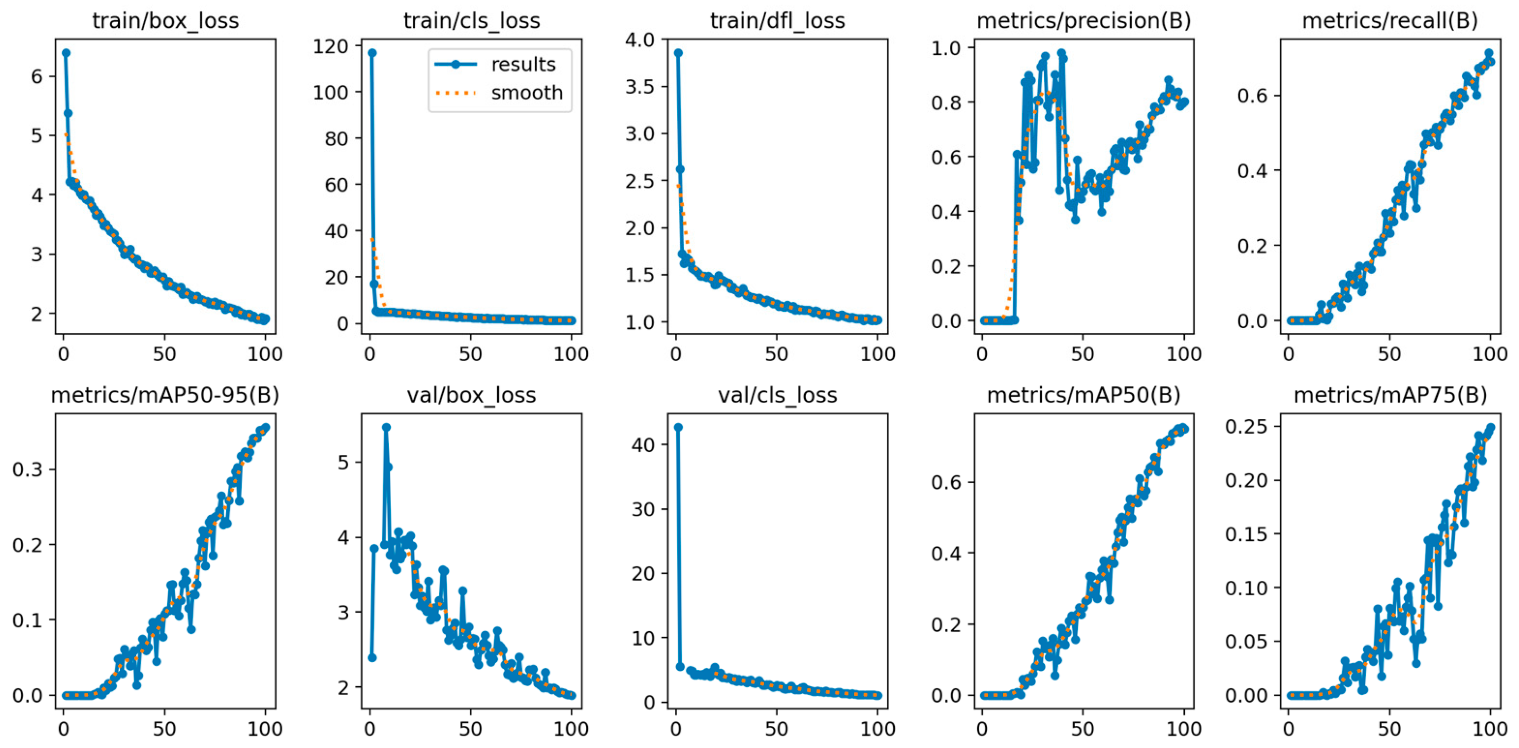
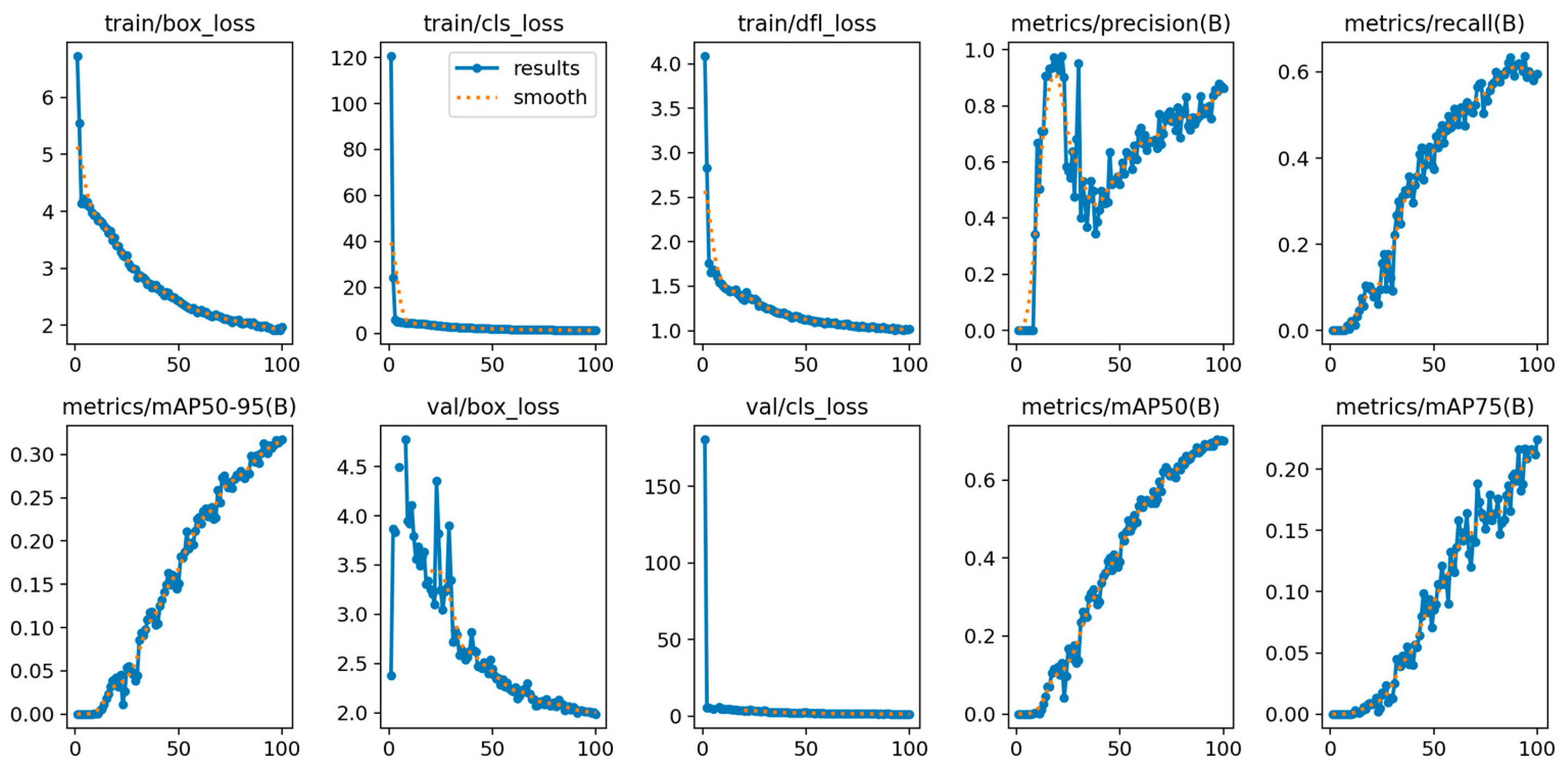
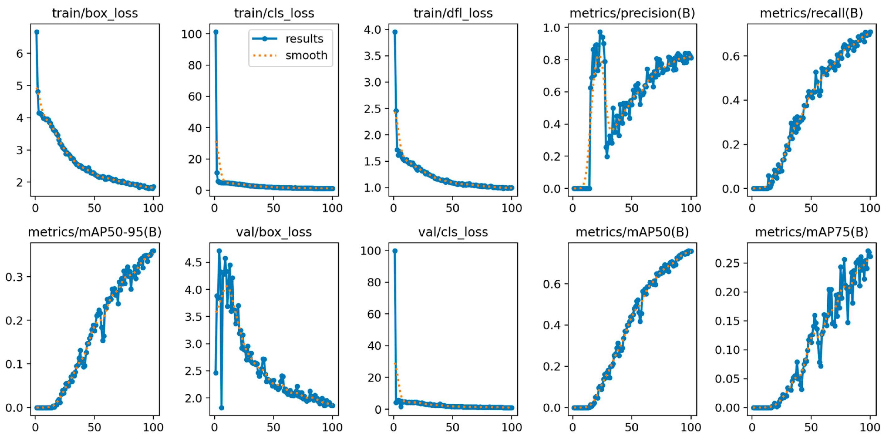
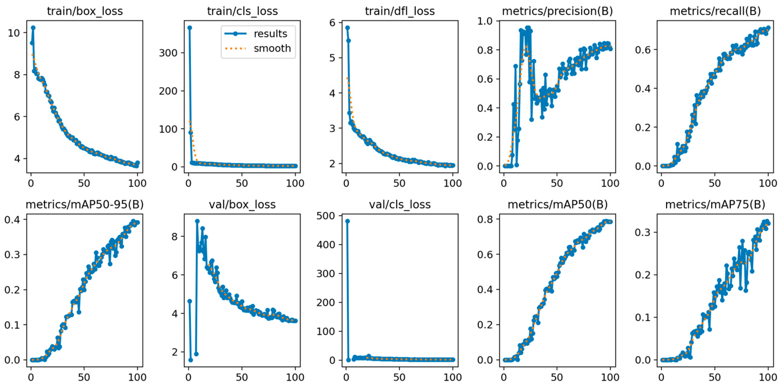
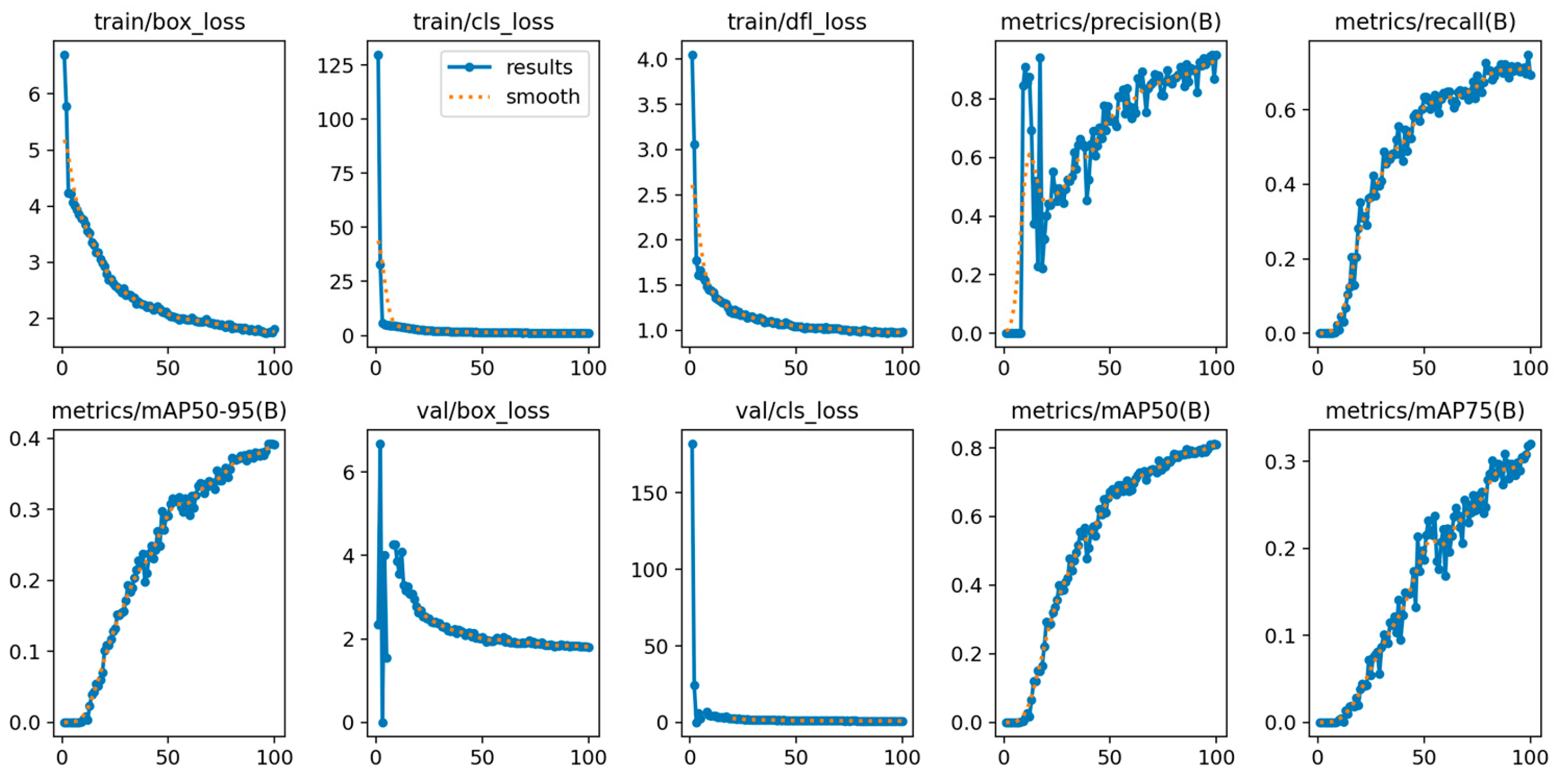
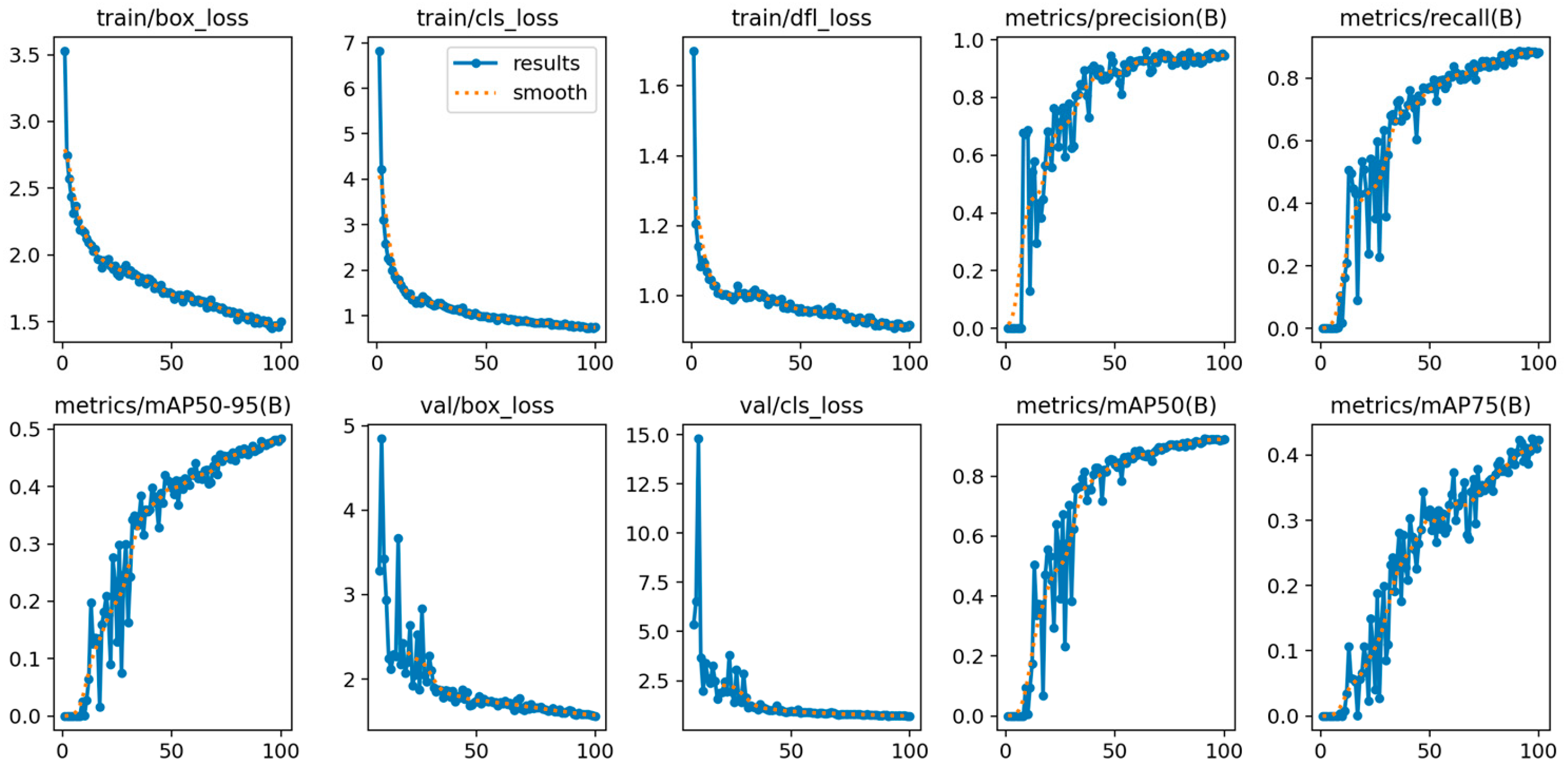
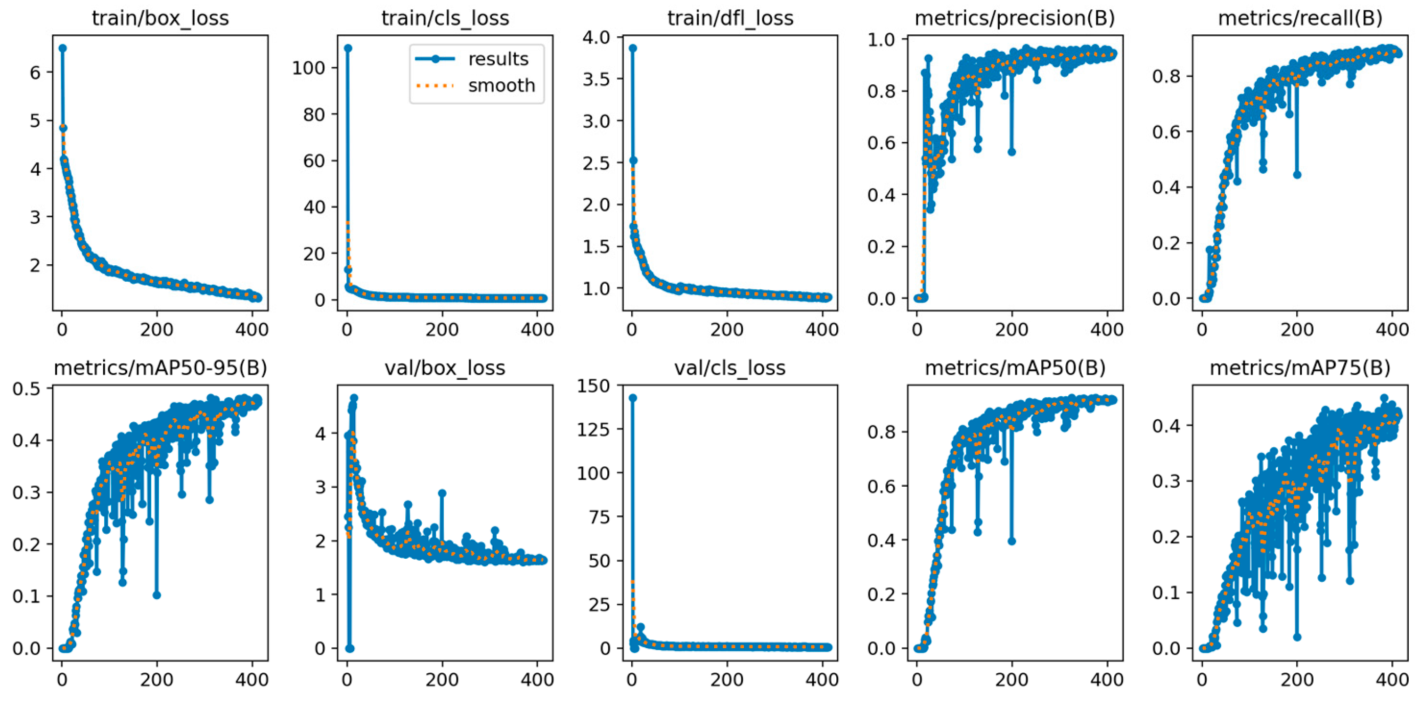
As designed above in Section 4.1, firstly, this paper evaluates the performance of six object detection algorithms, from YOLOv8 to YOLOv13, on PCB defect detection tasks under a unified training cycle (100 rounds) and a fixed dataset. The training analysis indicators are shown in Figure 1, Figure 2, Figure 3, Figure 4, Figure 5, Figure 6, Figure 7 and Figure 8, and the core evaluation indicators are shown in

Table 9. Core evaluation indicators of YOLO series algorithms in the 100-round experiments.

Specific Algorithms	M	GFLOPs	Inference (ms)	Other Indcators	All	Missing Hole	Mouse Bite	Open Circuit	Short Circuit	Spur	Spurious Copper
YOLOv8	3.01	8.1	0.5	P	0.810	0.994	0.752	0.804	0.688	0.783	0.836
				R	0.710	0.988	0.652	0.514	0.801	0.619	0.685
				mAP50	0.760	0.994	0.702	0.585	0.819	0.711	0.746
				mAP75	0.258	0.612	0.192	0.094	0.322	0.128	0.201
				mAP50-95	0.359	0.568	0.321	0.248	0.398	0.287	0.332
YOLOv9	7.17	26.7	2.1	P	0.796	0.971	0.806	0.597	0.818	0.746	0.837
				R	0.692	1.000	0.574	0.583	0.814	0.484	0.696
				mAP50	0.748	0.995	0.735	0.584	0.838	0.565	0.773
				mAP75	0.249	0.579	0.130	0.122	0.292	0.145	0.228
				mAP50-95	0.357	0.577	0.321	0.265	0.395	0.234	0.347
YOLOv10	8.04	24.5	1.5	P	0.813	0.940	0.850	0.715	0.762	0.790	0.818
				R	0.706	0.977	0.652	0.556	0.832	0.471	0.750
				mAP50	0.789	0.991	0.821	0.638	0.855	0.606	0.823
				mAP75	0.324	0.641	0.267	0.226	0.377	0.123	0.309
				mAP50-95	0.396	0.597	0.381	0.302	0.446	0.250	0.398
YOLOv11	2.58	6.3	0.6	P	0.864	0.981	0.879	0.827	0.834	0.856	0.805
				R	0.594	0.988	0.507	0.514	0.578	0.391	0.585
				mAP50	0.702	0.993	0.694	0.579	0.744	0.539	0.661
				mAP75	0.226	0.593	0.145	0.115	0.244	0.106	0.153
				mAP50-95	0.316	0.559	0.283	0.244	0.333	0.214	0.266
YOLOv12	2.51	5.8	0.9	P	0.869	0.778	0.919	0.813	0.897	0.925	0.884
				R	0.748	1.000	0.643	0.542	0.844	0.719	0.742
				mAP50	0.812	0.995	0.799	0.640	0.865	0.789	0.785
				mAP75	0.318	0.595	0.252	0.244	0.359	0.199	0.261
				mAP50-95	0.392	0.576	0.358	0.299	0.420	0.339	0.362
YOLOv13	2.45	6.2	1.1	P	0.945	0.992	0.985	0.872	0.939	0.955	0.926
				R	0.884	0.988	0.843	0.759	0.956	0.821	0.935
				mAP50	0.924	0.995	0.939	0.801	0.972	0.885	0.950
				mAP75	0.425	0.645	0.363	0.338	0.354	0.358	0.490
				mAP50-95	0.484	0.598	0.479	0.381	0.487	0.445	0.513

.

The results of the training analysis indicators and core evaluation indicators show that YOLOv13 significantly leads in most accuracy indicators (P = 0.945, R = 0.884, mAP50 = 0.924, and mAP50-95 = 0.484), while YOLOv8 and YOLOv12 achieve the best balance between efficiency and accuracy.

Performance comparison shows that YOLOv13 has the best comprehensive detection accuracy, especially in defects such as “mouse bite” (mAP50 = 0.939) and “open circuit” (mAP50 = 0.801), which are difficult to detect. YOLOv12 and YOLOv10 form the second tier, with mAP50 values of 0.812 and 0.789, respectively; YOLOv8 remains competitive (mAP50 = 0.760) and has the fastest inference speed (0.5 ms/image).

YOLOv9 and YOLOv11 are slightly inferior in overall performance (measured by mAP50). It is worth noting that YOLOv11 exhibits high accuracy (P = 0.864), ranking third among the six algorithms, only behind YOLOv13 (P = 0.945) and YOLOv12 (P = 0.869). However, its recall rate is relatively low (R = 0.594), which means that the model generates fewer FPs during the detection process, but relatively more FNs.

In terms of algorithm efficiency, the lightweight algorithms YOLOv11, YOLOv12, and YOLOv13 all have parameter sizes of about M = 2.5, with GFLOPs below 6.3, indicating high structural efficiency. Among them, YOLOv12 has the least number of parameters (M = 2.51) and the lowest computational cost (GFLOPs = 5.8), yet it achieves superior performance. On the contrary, the high-complexity YOLOv9 (M = 7.17, GFLOPs = 26.7) and YOLOv10 (M = 8.04, GFLOPs = 24.5) have not brought significant accuracy improvement and have lower practicality in edge deployment scenarios.

The results of various defect detection methods indicate that all algorithms almost perfectly detect “missing hole” (mAP50 > 0.99), and YOLOv13 also performs the best in types such as “short circuit” (mAP50 = 0.972) and “spur” (mAP50 = 0.885), highlighting its powerful ability to perceive subtle features and build contextual algorithms.

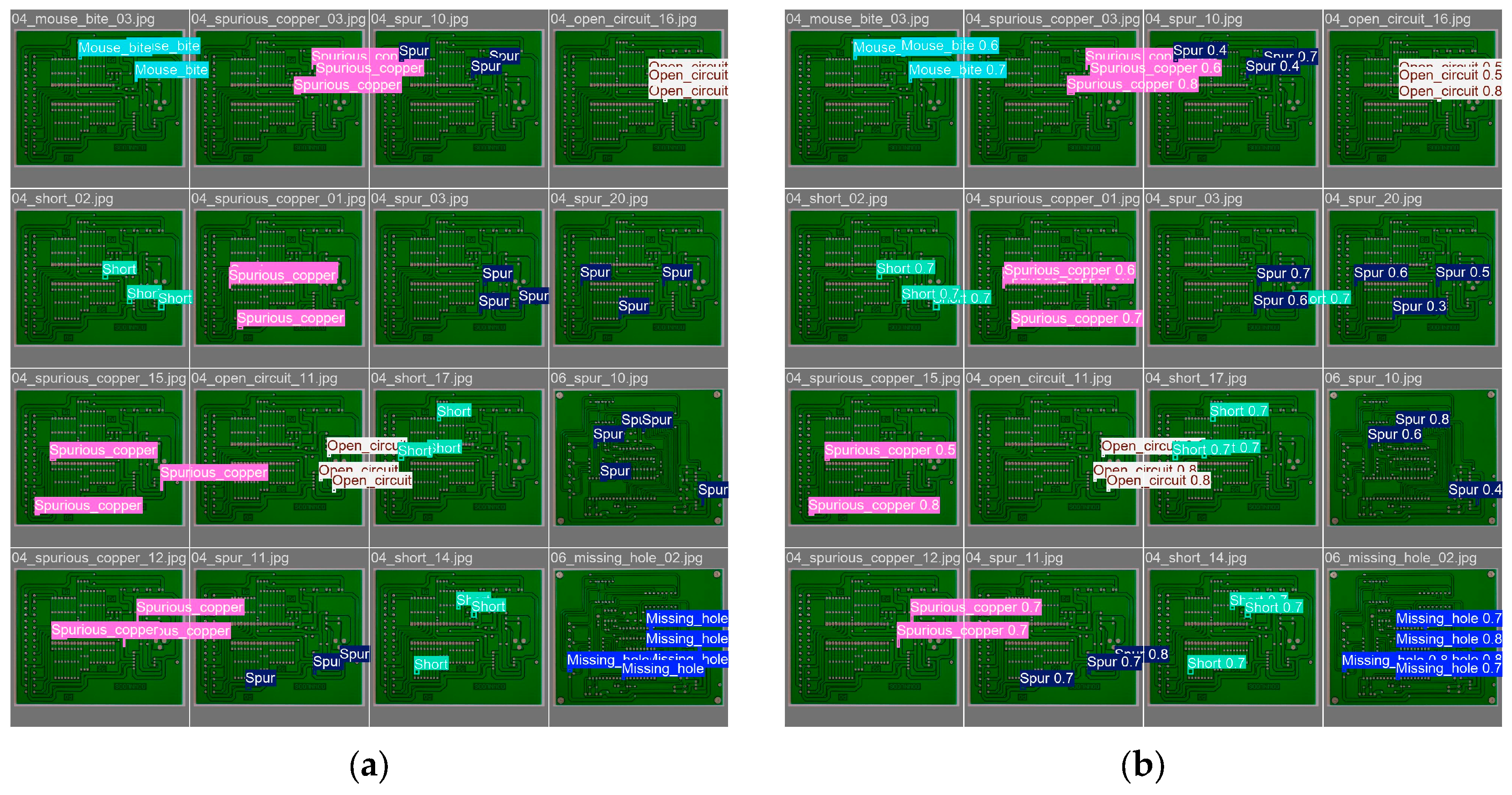
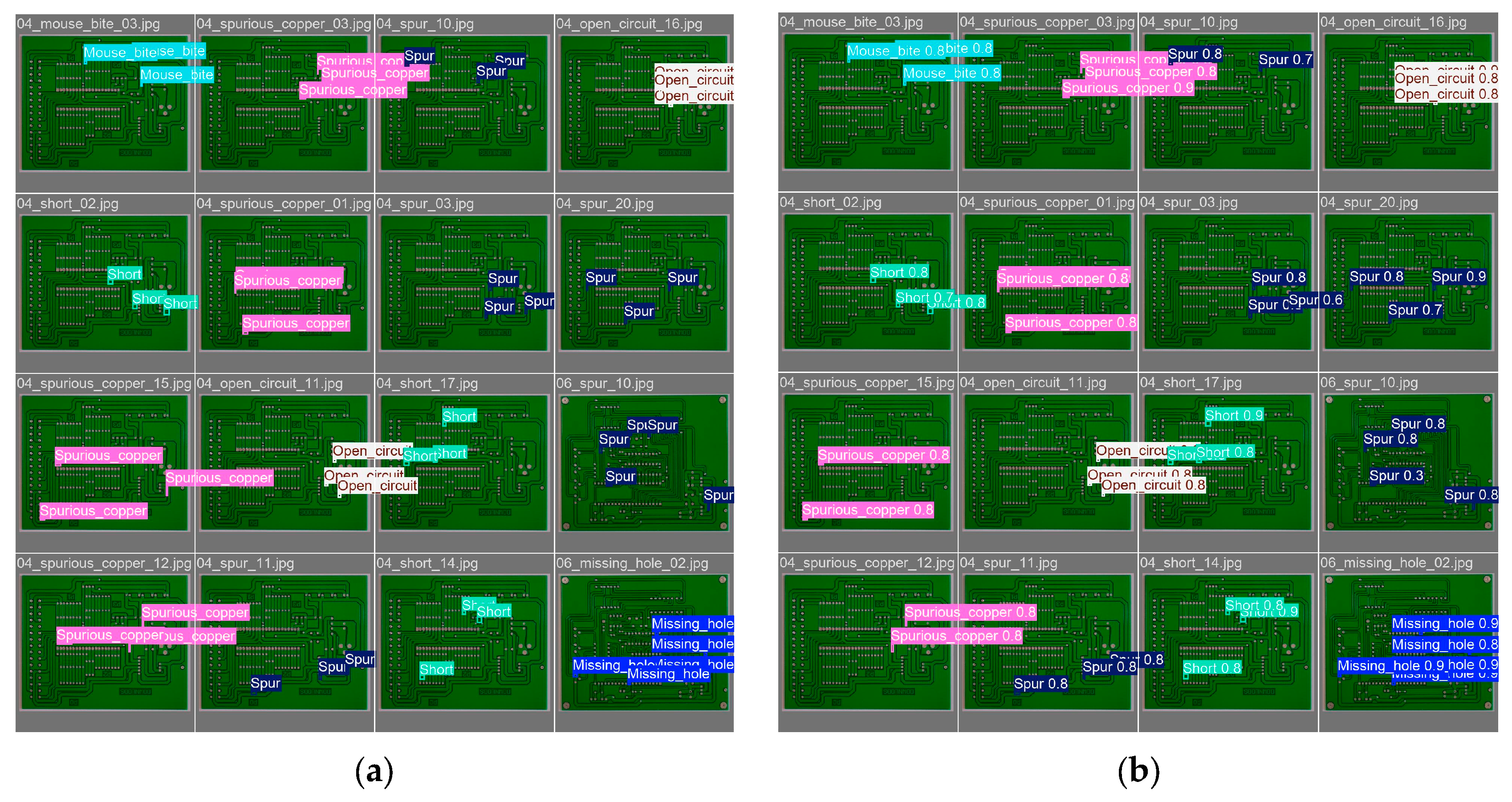
In summary, in scenarios where accuracy is prioritized and computing resources permit, it is recommended to use YOLOv13. The detection results are shown in Figure 9. In “efficiency first” scenarios that prioritize real-time performance and edge deployment, YOLOv8 and YOLOv12 are better choices. This part of the experiment confirms the highest level of accuracy of YOLOv13 in current PCB defect detection, and clarifies the efficiency and practicality of YOLOv8 and YOLOv12 in industrial practice.

4.3. 500 Rounds Experiment Results and Analysis

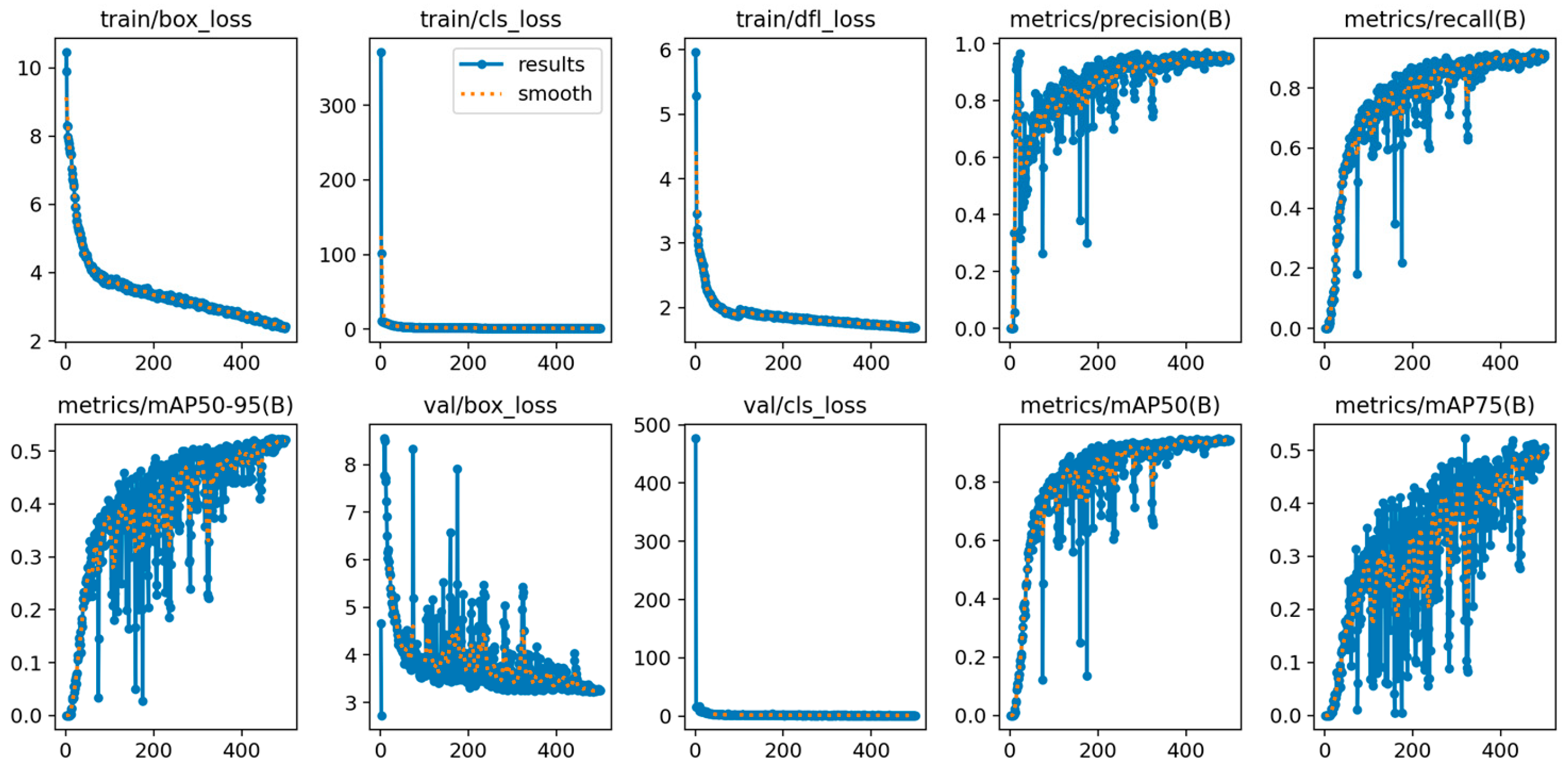
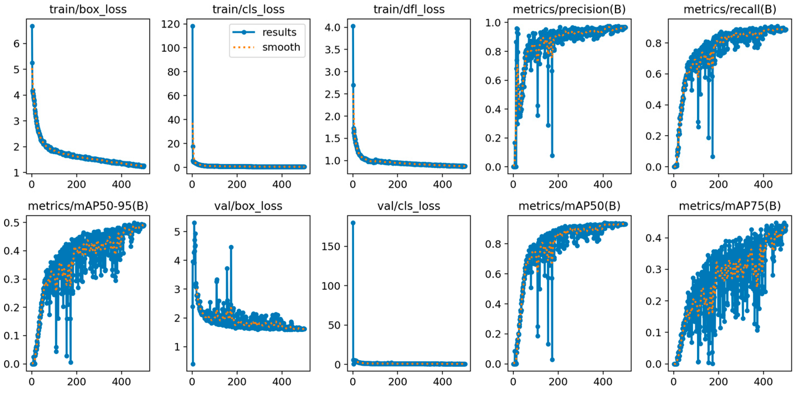
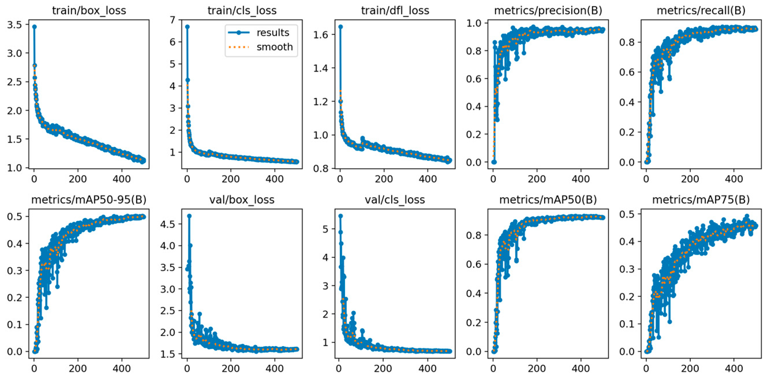
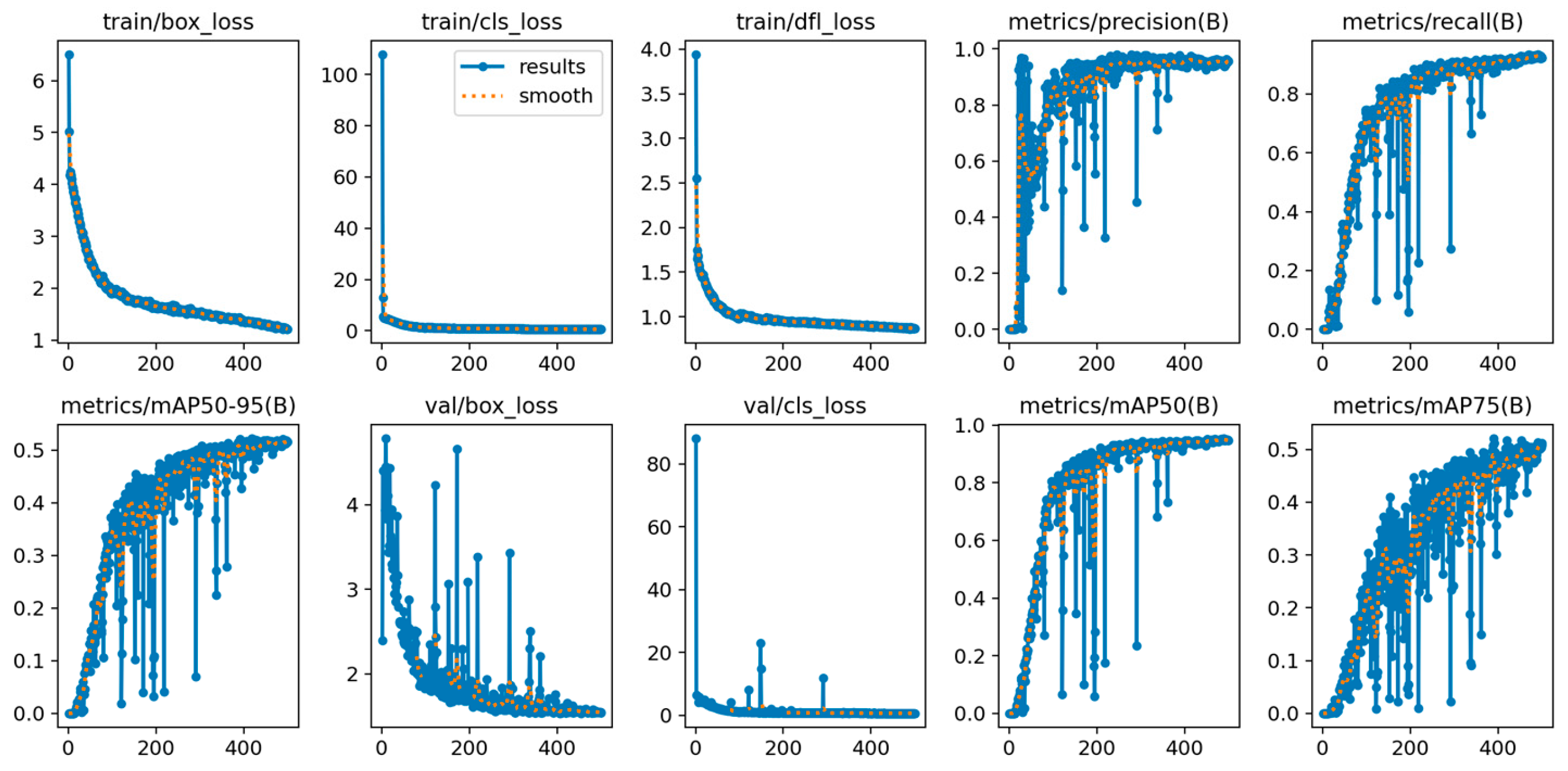
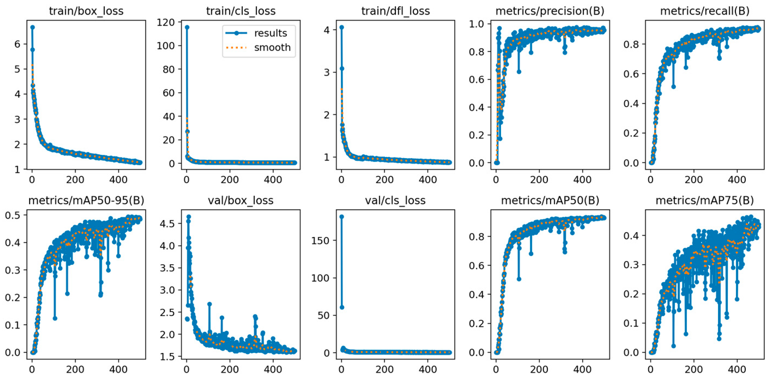
As designed above in Section 4.1, this paper also evaluates the performance of six object detection algorithms, from YOLOv8 to YOLOv13, on PCB defect detection tasks under a unified training cycle (500 rounds) and a fixed dataset. The training analysis indicators are shown from Figure 10, Figure 11, Figure 12, Figure 13, Figure 14, Figure 15, Figure 16 and Figure 17, and the core evaluation indicators are shown in

Table 10. Core evaluation indicators of YOLO series algorithms in the 500-round experiments.

Specific Algorithms	M	GFLOPs	Inference (ms)	Other Indcators	All	Missing Hole	Mouse Bite	Open Circuit	Short Circuit	Spur	Spurious Copper
YOLOv8	3.01	8.1	0.6	P	0.934	0.994	0.920	0.961	0.939	0.871	0.922
				R	0.885	1.000	0.861	0.736	0.952	0.836	0.924
				mAP50	0.918	0.995	0.922	0.819	0.939	0.874	0.957
				mAP75	0.418	0.638	0.424	0.352	0.396	0.312	0.384
				mAP50-95	0.482	0.588	0.467	0.423	0.483	0.427	0.501
YOLOv9	7.17	26.7	1.5	P	0.950	0.993	0.947	0.965	0.930	0.972	0.892
				R	0.916	1.000	0.930	0.806	0.973	0.820	0.967
				mAP50	0.939	0.995	0.969	0.862	0.954	0.881	0.971
				mAP75	0.514	0.656	0.494	0.444	0.528	0.415	0.550
				mAP50-95	0.520	0.588	0.531	0.459	0.531	0.462	0.551
YOLOv10	8.04	24.5	2.2	P	0.948	0.980	0.963	0.903	0.941	0.947	0.955
				R	0.909	1.000	0.902	0.792	0.947	0.867	0.946
				mAP50	0.946	0.995	0.967	0.840	0.971	0.924	0.977
				mAP75	0.508	0.779	0.489	0.332	0.487	0.433	0.526
				mAP50-95	0.526	0.623	0.522	0.443	0.544	0.478	0.543
YOLOv11	2.58	6.3	0.7	P	0.973	0.997	0.975	0.950	0.963	0.990	0.964
				R	0.884	1.000	0.843	0.806	0.927	0.803	0.924
				mAP50	0.939	0.995	0.936	0.852	0.963	0.913	0.973
				mAP75	0.447	0.741	0.427	0.274	0.376	0.420	0.446
				mAP50-95	0.498	0.633	0.489	0.391	0.496	0.466	0.515
YOLOv12	2.51	5.8	2.4	P	0.956	0.995	0.953	0.917	0.945	0.948	0.978
				R	0.896	1.000	0.872	0.750	0.947	0.860	0.948
				mAP50	0.931	0.995	0.953	0.803	0.944	0.914	0.976
				mAP75	0.463	0.740	0.468	0.297	0.514	0.334	0.422
				mAP50-95	0.495	0.617	0.492	0.388	0.521	0.436	0.514
YOLOv13	2.45	6.2	1.1	P	0.957	1.000	0.972	0.900	0.956	0.981	0.933
				R	0.886	0.999	0.894	0.747	0.960	0.810	0.904
				mAP50	0.928	0.995	0.951	0.791	0.978	0.891	0.961
				mAP75	0.478	0.765	0.512	0.274	0.406	0.433	0.478
				mAP50-95	0.502	0.625	0.521	0.384	0.510	0.466	0.508

.

The results show a significant change in the performance pattern of the algorithms after sufficient training: YOLOv10 is the best in comprehensive accuracy (mAP50-95 = 0.526), while YOLO11 has achieved the highest localization accuracy (0.973). YOLOv12 and YOLOv8 demonstrate outstanding efficiency, highlighting the diversity of algorithm selection.

Comprehensive performance analysis shows that YOLOv10 ranks first on mAP50-95 (0.526) and mAP50 (0.946), demonstrating robust and comprehensive detection capabilities. YOLO11 achieves near zero false positives with extremely high precision, but its recall rate (0.884) is relatively low. YOLOv9 achieves the highest recall rate (0.916) while maintaining high accuracy (0.950), demonstrating excellent recall capability for difficult samples.

The comparison of algorithm efficiency reveals a nonlinear relationship between performance and resource consumption. The lightweight algorithms YOLOv12 and YOLOv11 have significantly higher parameter sizes (M is about 2.5) and computational complexity (GFLOPs < 6.3), and YOLOv8 has the fastest inference speed (0.6 ms/image). Although the high-complexity algorithms YOLOv9 and YOLOv10 (with parameter count M > 7 and computational complexity GFLOPs > 24) achieve top-notch accuracy, they have heavy computational burden and slow inference speed (such as YOLOv10 being 2.2 ms/image). YOLOv13 strikes a balance between being lightweight (M = 2.45, GFLOPs = 6.2) and having excellent performance.

The evaluation of defect-specific detection capability shows that all algorithms almost perfectly detected “missing hole” (mAP50 > 0.995). YOLOv9 and YOLOv10 show the best performance in the “mouse bite” defect (mAP50 = 0.967 for both). In response to the most challenging “open circuit” defect, YOLOv9 leads with an mAP50 = 0.862. YOLOv11 has an extremely high accuracy rate (0.990) on “spur” defects, while YOLOv13 and YOLOv10 have achieved the best performance on “short circuit” and “spurious copper” defects, respectively.

In summary, if pursuing ultimate comprehensive accuracy and sufficient computing power, YOLOv10 is the first choice, and the target detection results are shown in Figure 18. In high-reliability scenarios with extremely low tolerance for false positives, YOLOv11 with the highest accuracy should be selected. In efficiency-sensitive edge deployment scenarios, YOLOv8 (fastest), YOLOv12 (lightest), and the well-balanced YOLOv13 are ideal choices.

The analysis of the impact of training cycles shows that algorithms with fast early convergence (such as YOLOv13 under 100 rounds of training) may not continue to lead after sufficient training, while some architectures (such as YOLOv10andYOLOv9) have achieved accuracy breakthroughs through long-term training. The advantage of lightweight algorithms in terms of computational efficiency is sustainable. This paper validated the scientific value of combining short-term screening and long-term evaluation through a dual-cycle comparison, providing a key basis for algorithm selection in industrial testing based on training resources, accuracy requirements, and deployment conditions.

4.4. Discussion

Although the experiment above provides a comprehensive and systematic empirical comparison of the performance of YOLO series algorithms from YOLOv8 to YOLOv13 in PCB defect detection, and draws a series of guiding conclusions for industrial algorithm selection, it should be noticed that any research has its specific boundaries and premises. The specific limitations of the above work should be pointed out as follows.

4.4.1. Dataset and Evaluation Scenarios

The limitations of datasets and evaluation scenarios are mainly reflected in the insufficient diversity of scenarios. The experiment of this paper is entirely based on the PKU-Market-PCB dataset collected under standard, uniform lighting, and static shooting conditions. Although this accurately simulates the ideal internal environment of AOI equipment, it fails to cover more complex and varied imaging conditions in real factories, such as drastically changing lighting, varying degrees of motion blur, and perspective distortion caused by tilted or uneven heights of the detected object. Therefore, the conclusion of this paper only accurately reflects the performance ranking of various algorithms in a “benchmark stable environment”, and their robustness and relative performance under extreme or non-standard imaging conditions still need to be specifically verified.

4.4.2. Algorithm Evaluation and Comparison Framework

To ensure fairness, all algorithms adopt a unified set of hyperparameters and training strategies that are close to default settings for preset configuration comparison. The advantage of this approach is that it controls variables, but the disadvantage is that it may not fully unleash the optimal potential of each algorithm. Some algorithms may achieve significant performance improvements through more refined hyperparameter tuning tailored to their architectural characteristics, such as learning rate scheduling, specific data augmentation strategies, and loss function weight adjustments. Therefore, the performance ranking of this paper should be understood as a benchmark evaluation under a unified methodological framework, rather than a final judgment on the theoretical performance limits of each algorithm.

On the other hand, this paper mainly relies on general target detection indicators such as mAP, accuracy, and recall. For the special field of industrial quality inspection, some business-oriented indicators are also crucial, such as the detection throughput per unit time (matching the production line pace), the comprehensive cost under different false/missed detection costs, and the detection rate of subtle defects. This paper does not include these business indicators in the quantitative category.

4.4.3. Algorithm Version Timeliness

In the field of DL, especially the YOLO series algorithms, updates and iterations are extremely rapid. This paper covers the major versions of the YOLO series from YOLOv8 to YOLOv13 that have been publicly released as of the time of submission, but updated versions such as YOLO26 are about to be officially released or are currently under development. The evaluation framework and methodology established in this paper have continuity value, but the specific performance ranking will dynamically change with technological development.

5. Conclusions and Future Prospects

5.1. Conclusions

With the development of electronic manufacturing towards high-density integration, automated defect detection of PCBs has become a key link in ensuring product quality. To solve the industrial algorithm selection problem caused by the rapid iteration of YOLO series algorithms, this paper has conducted a systematic dual-cycle (100 rounds and 500 rounds) empirical evaluation and comparative analysis of six state-of-the-art algorithms from YOLOv8 to YOLOv13 on a standardized PCB defect dataset for the first time. The experimental results show that the performance of the algorithm is highly dependent on the training period and performance dimension, and there is no universal optimal solution applicable to all scenarios.

Specifically, in the short-term, resource-limited training scenarios (100 rounds), YOLOv13 exhibits the fastest convergence ability and superior parameter efficiency, achieving comprehensive accuracy leadership with only M = 2.45 parameters in a few training rounds (mAP50 = 0.924, mAP50-95 = 0.484). This makes it the preferred choice for scenarios that require rapid prototyping validation or deployment time constraints. In a fully trained scenario (500 rounds) pursuing ultimate detection performance, YOLOv10 achieves the highest comprehensive detection accuracy, with mAP50 reaching 0.946 and mAP50-95 reaching 0.526, representing the current upper limit of accuracy for the YOLO series in this task. Meanwhile, YOLOv9 performs the best in positioning accuracy (mAP75), reaching 0.514. In terms of efficiency and accuracy balance, YOLOv11 achieves the best speed accuracy balance after long-term training (accuracy = 0.973, inference speed = 0.7 ms/graph), which is very suitable for high-throughput online detection production lines. YOLOv12, on the other hand, demonstrates excellent lightweight characteristics (parameter size M = 2.51, GFLOPs = 5.8) and good initial accuracy (mAP50 = 0.812) during short-term training. Regarding the difficulty of defect detection, this paper quantitatively reveals that “open circuit” and “spur” are the most challenging types among the six typical defects through cross algorithm consistency analysis. Under 100 rounds of training, the average mAP50 of all algorithms for the “open circuit” defect is only 0.638, and for the “spur” defect is only 0.683, far lower than the almost-perfect detection of “missing holes” (mAP50 > 99%), which points to a key direction for future data augmentation and algorithm optimization.

This paper provides a clear and actionable decision-making basis for algorithm selection in the industry under different constraints, such as training resources, real-time requirements, and accuracy priority, through rigorous benchmark testing. The established evaluation framework and performance map not only provide direct guidance for the design and optimization of PCB AOI systems, but also set new performance reference standards for precision visual quality inspection of electronic components more widely. Future work can further explore the performance of algorithms in more complex defects, extremely small targets, and cross domain generalization ability, in order to continuously promote the deep application and reliability improvement of intelligent detection technology in the field of electronic manufacturing.

5.2. Future Prospects

Taking into account the relevant conclusions already obtained in this paper and the research limitations discussed in Section 4.4, future research can be conducted in the following directions. Firstly, more challenging evaluation benchmarks can be constructed to promote the establishment of an open-source PCB defect detection dataset that includes diverse imaging conditions, more comprehensive defect types, and larger data volumes, in order to facilitate the advancement of algorithms in real-world complexity and robustness. Secondly, on the basis of controlling variables, targeted hyperparameter optimization research can be conducted to explore the performance limits of each algorithm; at the same time, the evaluation can be extended to a wider range of edge hardware platforms and business indicators directly related to production pace and quality costs can be introduced. Thirdly, researching technical paths to improve the generalization and adaptability of algorithms can be studied; techniques such as domain adaptation, test time augmentation, and meta learning can be explored to enhance the rapid adaptation and stable performance of pre-trained models in new scenarios and lighting conditions. Last but not least, the automation mechanism for algorithm selection and configuration can be explored; based on the data accumulated from this paper and subsequent richer benchmark tests, an automated algorithm recommendation system can be explored to automatically recommend the most suitable detection algorithm and initial configuration according to user-specific hardware constraints, accuracy requirements, defect type preferences, and other inputs.

References

1. Wang, Y.; Wang, J.; Cao, Y.; Li, S.; Kwan, O. Integrated inspection of PCB manufacturing in cyber-physical-social systems. IEEE Trans. Syst. Man Cybern. Syst. 2023, 53, 2098–2106. [Google Scholar] [CrossRef] [Scilit]
2. Wang, W.C.; Chen, S.L.; Chen, L.B.; Chang, W.J. A machine vision based automatic optical inspection system for measuring drilling quality of printed circuit boards. IEEE Access 2017, 5, 10817–10833. [Google Scholar] [CrossRef] [Scilit]
3. Wu, H.; Lei, R.; Peng, Y. PCBNet: A lightweight convolutional neural network for defect inspection in surface mount technology. IEEE Trans. Instrum. Meas. 2022, 71, 3518314. [Google Scholar] [CrossRef] [Scilit]
4. Cao, Y.; Wang, Y.; Wang, J.; Tian, Y.; Wang, X.; Wang, F.Y. Parameter identification and refinement for parallel PCB inspection in cyber-physical-social systems. IEEE Trans. Comput. Soc. Syst. 2024, 11, 3978–3987. [Google Scholar] [CrossRef] [Scilit]
5. Deng, L.; Meng, X.; Guo, X.; Chen, Y.; Shan, H.; Wu, S.; Lin, J.; Dong, M.; Zhu, L. Learned optical flow-based defect detection with coarse-to-fine nonrigid image alignment. IEEE Sens. J. 2025, 25, 8684–8696. [Google Scholar] [CrossRef] [Scilit]
6. Zhou, W.; Li, C.; Ye, Z.; He, Q.; Ming, Z.; Chen, J. An efficient tiny defect detection method for PCB with improved YOLO through a compression training strategy. IEEE Trans. Instrum. Meas. 2024, 73, 2003514. [Google Scholar] [CrossRef] [Scilit]
7. Mo, C.; Hu, Z.; Wang, J.; Xiao, X. SGT-YOLO: A lightweight method for PCB defect detection. IEEE Trans. Instrum. Meas. 2025, 74, 3543911. [Google Scholar] [CrossRef] [Scilit]
8. Li, K.; Zhong, X.; Han, Y. A high-performance small target defect detection method for PCB boards based on a novel YOLO-DFA algorithm. IEEE Trans. Instrum. Meas. 2025, 74, 2008312. [Google Scholar] [CrossRef] [Scilit]
9. He, X.; Xie, M. ABF-YOLO: A fine-grained PCB defect detection framework integrating axial attention and bidirectional feature fusion. IEEE Trans. Consum. Electron. 2025, 71, 8562–8570. [Google Scholar] [CrossRef] [Scilit]
10. Wu, H.; Lin, Y. A high-performance and enhanced generalization small target defect detection method for PCB boards based on YOLO-EMAC. IEEE Trans. Instrum. Meas. 2025, 74, 5042513. [Google Scholar] [CrossRef] [Scilit]
11. Redmon, J.; Divvala, S.; Girshick, R.; Farhadi, A. You only look once: Unified, real-time object detection. In Proceedings of the IEEE Conference on Computer Vision and Pattern Recognition (CVPR), Las Vegas, NV, USA, 27–30 June 2016. [Google Scholar] [CrossRef] [Scilit]
12. Redmon, J.; Farhadi, A. YOLO9000: Better, faster, stronger. In Proceedings of the IEEE Conference on Computer Vision and Pattern Recognition (CVPR), Honolulu, HI, USA, 21–26 July 2017. [Google Scholar] [CrossRef] [Scilit]
13. Redmon, J.; Farhadi, A. Yolov3: An incremental improvement. arXiv 2018, arXiv:1804.02767. [Google Scholar] [CrossRef] [Scilit]
14. Bochkovskiy, A.; Wang, C.Y.; Liao, H.Y.M. Yolov4: Optimal speed and accuracy of object detection. arXiv 2020, arXiv:2004.10934. [Google Scholar] [CrossRef] [Scilit]
15. Jocher, G.; Liu, C.; Hogan, A.; Yu, L.; Rai, P.; Sullivan, T. Ultralytics/Yolov5: Initial Release, version 1.0; Zenodo: Geneva, Switzerland, 2020.
16. Li, C.; Li, L.; Jiang, H.; Weng, K.; Geng, Y.; Li, L.; Ke, Z.; Li, Q.; Cheng, M.; Nie, W.; et al. YOLOv6: A single-stage object detection framework for industrial applications. arXiv 2022, arXiv:2209.02976. [Google Scholar] [CrossRef] [Scilit]
17. Wang, C.Y.; Bochkovskiy, A.; Liao, H.Y.M. YOLOv7: Trainable bag-of-freebies sets new state-of-the-art for real-time object detectors. In Proceedings of the IEEE/CVF Conference on Computer Vision and Pattern Recognition (CVPR), Vancouver, BC, Canada, 17–24 June 2023. [Google Scholar] [CrossRef] [Scilit]
18. YOLOv8. Available online: https://github.com/dme-compunet/YoloSharp (accessed on 6 December 2025).
19. Wang, C.Y.; Yeh, I.H.; Liao, H.Y.M. YOLOv9: Learning what you want to learn using programmable gradient information. arXiv 2024, arXiv:2402.13616. [Google Scholar] [CrossRef] [Scilit]
20. Wang, A.; Chen, H.; Liu, L.; Chen, K.; Lin, Z.; Han, J.; Ding, G. YOLOv10: Real-time end-to-end object detection. arXiv 2024, arXiv:2405.14458. [Google Scholar]
21. YOLOv11. Available online: https://github.com/yt7589/yolov11 (accessed on 6 December 2025).
22. Tian, Y.; Ye, Q.; Doermann, D. YOLOv12: Attention-centric real-time object detectors. arXiv 2025, arXiv:2502.12524. [Google Scholar]
23. Lei, M.; Li, S.; Wu, Y.; Hu, H.; Zhou, Y.; Zheng, X.; Ding, G.; Du, S.; Wu, Z.; Gao, Y. YOLOv13: Real-time object detection with hypergraph-enhanced adaptive visual perception. arXiv 2025, arXiv:2506.17733. [Google Scholar]
24. Sapkota, R.; Cheppally, R.H.; Sharda, A.; Karkee, M. YOLO26: Key architectural enhancements and performance benchmarking for real-time object detection. arXiv 2025, arXiv:2509.25164. [Google Scholar] [CrossRef] [Scilit]
25. Bhavana, N.; Kodabagi, M.M.; Kumar, B.M.; Ajay, P.; Muthukumaran, N.; Ahilan, A. POT-YOLO: Real-time road potholes detection using edge segmentation-based Yolo V8 network. IEEE Sens. J. 2024, 24, 24802–24809. [Google Scholar] [CrossRef] [Scilit]
26. Zhong, J.; Kong, D.; Wei, Y.; Pan, B. YOLOv8 and point cloud fusion for enhanced road pothole detection and quantification. Sci. Rep. 2025, 15, 11260. [Google Scholar] [CrossRef] [Scilit]
27. Moussaoui, H.; Akkad, N.E.; Benslimane, M.; El-Shafai, W.; Baihan, A.; Hewage, C.; Rathore, R.S. Enhancing automated vehicle identification by integrating YOLO v8 and OCR techniques for high-precision license plate detection and recognition. Sci. Rep. 2024, 14, 14389. [Google Scholar] [CrossRef] [Scilit] [PubMed]
28. Yi, H.; Liu, B.; Zhao, B.; Liu, E. Small object detection algorithm based on improved YOLOv8 for remote sensing. IEEE J. Sel. Top. Appl. Earth Obs. Remote Sens. 2024, 17, 1734–1747. [Google Scholar] [CrossRef] [Scilit]
29. Bakirci, M.; Bayraktar, I. Transforming aircraft detection through LEO satellite imagery and YOLOv9 for improved aviation safety. In Proceedings of the 26th International Conference on Digital Signal Processing and its Applications (DSPA), Moscow, Russia, 27–29 March 2024. [Google Scholar] [CrossRef] [Scilit]
30. Ma, R.; Yu, H.; Liu, X.; Yuan, X.; Geng, T.; Li, P. InSAR-YOLOv8 for wide-area landslide detection in InSAR measurements. Sci. Rep. 2025, 15, 1595. [Google Scholar] [CrossRef] [Scilit] [PubMed]
31. Ma, C.; Chi, G.; Ju, X.; Zhang, J.; Yan, C. YOLO-CWD: A novel model for crop and weed detection based on improved YOLOv8. Crop Prot. 2025, 192, 107169. [Google Scholar] [CrossRef] [Scilit]
32. Regotra, R.; Kumar, R. YOLOv8-based early blight and late blight disease detection in potato. In Proceedings of the 15th International Conference on Computing Communication and Networking Technologies (ICCCNT), Kamand, India, 24–28 June 2024. [Google Scholar] [CrossRef] [Scilit]
33. Srivastava, A.; Singh, G.; Bhatnagar, V.; Shrivastava, V.; Grag, N. Method for detecting potato leaf disease using the YOLOv8 model. In Proceedings of the International Conference on Signal Processing and Advance Research in Computing (SPARC), Lucknow, India, 12–13 September 2024. [Google Scholar] [CrossRef] [Scilit]
34. Safre, A.L.S.; Torres-Rua, A.; Black, B.L.; Young, S. Deep learning framework for fruit counting and yield mapping in tart cherry using YOLOv8 and YOLO11. Smart Agric. Technol. 2025, 11, 100948. [Google Scholar] [CrossRef] [Scilit]
35. Dai, Q.; Liang, S.; Li, Z.; Lyu, S.; Xue, X.; Song, S.; Huang, Y.; Zhang, S.; Fu, J. YOLOv11-RDTNet: A lightweight model for citrus pest and disease identification based on an improved YOLOv11n. Agronomy 2025, 15, 1252. [Google Scholar] [CrossRef] [Scilit]
36. Sapkota, R.; Cheppally, R.H.; Sharda, A.; Karkee, M. RF-DETR object detection vs YOLOv12: A study of Transformer-based CNN-based architectures for single-class and multi-class greenfruit detection in complex orchard environments under label ambiguity. arXiv 2025, arXiv:2504.13099. [Google Scholar] [CrossRef] [Scilit]
37. Sapkota, R.; Ahmed, D.; Karkee, M. Comparing YOLOv8 and mask R-CNN for instance segmentation in complex orchard environments. Artif. Intell. Agric. 2024, 13, 84–99. [Google Scholar] [CrossRef] [Scilit]
38. Zhu, W.; Niu, S.; Yue, J.; Zhou, Y. Multiscale wildfire and smoke detection in complex drone forest environments based on YOLOv8. Sci. Rep. 2025, 15, 2399. [Google Scholar] [CrossRef] [Scilit]
39. Wang, H.; Fu, X.; Yu, Z.; Zeng, Z. DSS-YOLO: An improved lightweight real-time fire detection model based on YOLOv8. Sci. Rep. 2025, 15, 8963. [Google Scholar] [CrossRef] [Scilit]
40. Ramos, L.; Casas, E.; Bendek, E.; Romero, C.; Rivas-Echeverriia, F. Hyperparameter optimization of YOLOv8 for smoke and wildlife detection: Implications for agricultural and environmental safety. Artif. Intell. Agric. 2024, 12, 109–126. [Google Scholar] [CrossRef] [Scilit]
41. Cai, Y.; Chen, L.; Zhuang, X.; Zhang, B. Automated marine oil spill detection algorithm based on single-image generative adversarial network and YOLO-v8 under small samples. Mar. Pollut. Bull. 2024, 203, 116475. [Google Scholar] [CrossRef] [Scilit] [PubMed]
42. Shankar, G.; Geetha, M.K.; Ezhumalai, P. Disaster management systems: Utilizing YOLOv9 for precise monitoring of river flood flow levels using video surveillance. SN Comput. Sci. 2025, 6, 288. [Google Scholar] [CrossRef] [Scilit]
43. Liu, B.; Li, Y.; Feng, X.; Lian, P. BEW-YOLOv8: A deep learning model for multi-scene and multi-scale flood depth estimation. J. Hydrol. 2024, 645, 132139. [Google Scholar] [CrossRef] [Scilit]
44. Chen, L.; Li, G.; Zhang, S.; Mao, W.; Zhang, M. YOLO-SAG: An improved wildlife object detection algorithm based on YOLOv8n. Ecol. Inform. 2024, 83, 102791. [Google Scholar] [CrossRef] [Scilit]
45. Pan, W.; Chen, J.; Lv, B.; Peng, L. Lightweight marine biodetection model based on improved YOLOv10. Alex. Eng. J. 2025, 119, 379–390. [Google Scholar] [CrossRef] [Scilit]
46. Wang, X.; Song, X.; Li, Z.; Wang, H. YOLO-DBS: Efficient target detection in complex underwater scene images based on improved YOLOv8. J. Ocean Univ. China 2025, 24, 979–992. [Google Scholar] [CrossRef] [Scilit]
47. Gui, H.; Su, T.; Jiang, X.; Li, L.; Xiong, L.; Zhou, J.; Pang, Z. FS-YOLOv9: A frequency and spatial feature-based YOLOv9 for real-time breast cancer detection. Acad. Radiol. 2025, 32, 1228–1240. [Google Scholar] [CrossRef] [Scilit]
48. Liu, Z.; Wei, L.; Song, T. Optimized YOLOv11 model for lung nodule detection. Biomed. Signal Process. Control 2025, 107, 107830. [Google Scholar] [CrossRef] [Scilit]
49. Srinivasu, P.N.; Kumari, G.L.A.; Narahari, S.C.; Ahmed, S.; Alhumam, A. Exploring the impact of hyperparameter and data augmentation in YOLO V10 for accurate bone fracture detection from X-ray images. Sci. Rep. 2025, 15, 9828. [Google Scholar] [CrossRef] [Scilit]
50. IPC-A-600 Acceptability of Printed Boards (in Chinese), the Current Latest Edition IPC-A-600K. Available online: https://www.ipc.org.cn/productinfo/1307827.html (accessed on 9 January 2026).
Figure 1. Training analysis indicators of YOLOv8 in the100-round experiment.
Machines 14 00094 g001
Figure 2. Training analysis indicators of YOLOv9 in the100-round experiment.
Machines 14 00094 g002
Figure 3. Training analysis indicators of YOLOv10 in the100-round experiment.
Machines 14 00094 g003
Figure 4. Training analysis indicators of YOLOv11 in the100-roundexperiment.
Machines 14 00094 g004
Figure 5. Training analysis indicators of YOLOv12 in the100-round experiment.
Machines 14 00094 g005
Figure 6. Training analysis indicators of YOLOv13 in the100-round experiment.
Machines 14 00094 g006
Figure 7. Normalized confusion matrices in the 100-round experiments. (a) YOLOv8; (b) YOLOv9; (c) YOLOv10; (d) YOLOv11; (e) YOLOv12; and (f) YOLOv13.
Machines 14 00094 g007
Figure 8. F1 confidence curves in the 100-round experiments. (a) YOLOv8; (b) YOLOv9; (c) YOLOv10; (d) YOLOv11; (e) YOLOv12; and (f) YOLOv13.
Machines 14 00094 g008
Figure 9. Object detection results of YOLOv13 in the100-roundexperiment: (a) defects marked; (b) defects detected out.
Machines 14 00094 g009
Figure 10. Training analysis indicators of YOLOv8 in the 500-round experiment.
Machines 14 00094 g010
Figure 11. Training analysis indicators of YOLOv9 in the 500-round experiment.
Machines 14 00094 g011
Figure 12. Training analysis indicators of YOLOv10 in the 500-round experiment.
Machines 14 00094 g012
Figure 13. Training analysis indicators of YOLOv11 in the 500-round experiment.
Machines 14 00094 g013
Figure 14. Training analysis indicators of YOLOv12 in the 500-round experiment.
Machines 14 00094 g014
Figure 15. Training analysis indicators of YOLOv13 in the 500-round experiment.
Machines 14 00094 g015
Figure 16. Normalized confusion matrices in the500-round experiments. (a) YOLOv8; (b) YOLOv9; (c) YOLOv10; (d) YOLOv11; (e) YOLOv12; and (f) YOLOv13.
Machines 14 00094 g016aMachines 14 00094 g016b
Figure 17. F1 confidence curves in the 500-round experiment. (a) YOLOv8; (b) YOLOv9; (c) YOLOv10; (d) YOLOv11; (e) YOLOv12; and (f) YOLOv13.
Machines 14 00094 g017aMachines 14 00094 g017b
Figure 18. Object detection results of YOLOv10 in the 500-round experiments: (a) defects marked; (b) defects detected out.
Machines 14 00094 g018