Abstract
Controlling autonomous vehicles to follow a desired lateral trajectory presents a significant challenge. Developers of lateral control systems often find it difficult to simultaneously bring both lateral error and heading angle error close to zero while smoothly following the curvature of the road. This paper introduces the design and development of a control strategy for lateral trajectory following using the backstepping control method, which successfully achieves the goal of stabilization and tracking. The controller comprises a backstepping feedback control law to regulate the errors and stabilize the vehicle by controlling the yaw rate, along with a dynamic feedforward component to compensate for road curvature and further eliminate steady-state errors on curved roads. The controller is built upon the dynamic bicycle model, enhanced by integrating the error dynamics into the state space equation, which allows for the inclusion of errors as state variables. The global uniform stability of the feedback control law is proven using Lyapunov stability theory and the LaSalle–Yoshizawa theorem. The stability and tracking performance of the controller are validated through simulation and experimental results obtained from a test vehicle on a public highway.
1. Introduction
Interest in the field of autonomous vehicles has increased tremendously in the last decade due to the increasing demand for safety, mobility, and convenient driving. Trajectory tracking control serves as a fundamental and essential function for autonomous vehicles. The Trajectory Tracking Controller (TTC) governs the vehicle’s motion in both lateral and longitudinal dimensions. Utilizing data from vision sensors like cameras, lidar, and radar, the environmental model formulates an optimal and safe trajectory for the vehicle to adhere to. The longitudinal TTC is responsible for managing the vehicle’s longitudinal position and speed, while the lateral TTC handles the lateral position and heading angle, ensuring the vehicle navigates the road’s curvature correctly. This paper specifically concentrates on the lateral TTC aspect. As shown in Figure 1, the lateral TTC factors in both the lateral deviation and the heading angle deviation of the vehicle relative to its intended path, along with the road curvature. This information is used to calculate the necessary steering angle to correct any discrepancies from the desired trajectory and to navigate the road’s curvature. The requested steering angle is then communicated to the steering angle controller, which determines the required torque to activate the electric power steering, enabling the wheel to adjust to the requested angle by the lateral TTC. The steering angle controller design and development are not discussed in this paper, and a detailed design and development with experimental results can be found in [1].

Figure 1.
Lateral Control Block Diagram.
Backstepping (BS) is an effective recursive control strategy based on Lyapunov’s method. It is suitable for both linear and nonlinear systems in strict feedback form. This method was first introduced and explored by Krstic, Kanellakopoulos, and Kokotovic in the early 1990s in their work [2]. The core concept of backstepping involves recursively designing a controller by treating certain state variables as independent virtual controls, allowing us to design intermediate stabilizing control laws for them. During this design process, we break down the system into smaller subsystems, stabilizing each one individually by developing a Lyapunov function for it. Ultimately, we formulate a Lyapunov function to ensure stability for the entire system. Backstepping is known for its regulation and tracking capabilities while stabilizing the controlled system asymptotically. It can achieve those properties without canceling useful nonlinearities, as in the case of feedback linearization, and without producing destabilizing nonlinear terms in the control law [2]. An example of useful nonlinearities is signals that are raised to an odd power; they contribute to the feedback control law by adding damping for large values of the signal. However, the presence of those variables may lead to a large control effort, which makes them undesirable for systems with actuator limitations.
The backstepping control method has been widely used for trajectory following of different types of mobile robots at low speeds and using kinematic models; some of this work can be found in [3,4,5,6]. It has also been used in controlling autonomous underwater vehicles [7,8,9]. In our paper, backstepping is applied for highway autonomous vehicles at highway speeds of 60–70 mph and using a dynamical vehicle model. Sliding mode control (SMC) has been investigated for TTC [10,11,12,13]. The drawback of the sliding mode control is that it introduces undesirable vibrations called chattering, caused by the discontinuous part of the sliding mode control law. Even though there are some techniques to mitigate the chattering, such as the super twisting SMC [10], replacing the sign function by a saturation function [12], it will always exist because it can be reduced but not eliminated totally, especially in real time, when the controller is tested in the real vehicle. Furthermore, decreasing it comes at a price, impacting both the bandwidth of the controller and its tracking ability. While chattering is tolerable in electrical systems where the control input is voltage, it is not deemed acceptable in mechanical systems when the control input is torque, and since the steering angle command coming from the TTC will be converted to steering torque acting on the steering wheel, the chattering will be seen and felt by the driver. In [10], a combination of super-twisting SMC and backstepping control is developed to control the trajectory following of autonomous vehicles, where the control law is developed using SMC, and the backstepping is only used to prove the stability of the control system. One limitation of the control strategy in [10] is that it only controls the lateral deviation (lateral offset of the vehicle from the center of the trajectory) and vehicle yaw rate, but does not control the vehicle yaw angle (heading angle). Without controlling the yaw angle of the vehicle to follow the direction of the road, the trajectory tracking control will be poor at curved roads. Another limitation in [10,11,12,13], as in many other research papers, is that there is no feedforward strategy to compensate for curved roads. Feedforward is very important for computing the steering angle required to negotiate curved roads. The lack of yaw angle control and feedforward explains the deviation of the vehicle trajectory from the desired trajectory in figure 11 in [10]; much more accuracy is needed in real time at highway speeds for safety. They might not look that bad in Carsim and hardware in the loop (HIL) simulation, but these problems will become much more serious and might cause instability of the trajectory following when it comes to the real-time implementation in the real vehicle at highway speeds.
Various algorithms have been examined in the existing literature for Lateral TTC. Among the most widely recognized are the geometry-based Stanley method [14,15] and the Pure Pursuit technique [16,17,18]. Both of these approaches utilize the kinematic bicycle model. However, a significant limitation of the kinematic bicycle model is its failure to account for dynamic lateral forces acting on the vehicle, as it disregards the tire slip angle. This model performs adequately at low speeds, where the slip angle is nearly zero, but as speed rises, lateral acceleration and forces also increase, leading to a non-zero tire slip angle. Due to its inability to account for these lateral forces, the performance of the controller diminishes. Additionally, geometry-based controllers struggle on roads with high curvature, largely because the reference dynamics were not incorporated in the development of the kinematic model. The concept of Model Predictive Control (MPC) has also been investigated in [19,20,21,22,23,24]. MPC is a powerful optimal control method, but it may raise high computational complexity issues in production vehicles because it is a numerical method that computes a new solution at every time step, unlike analytical methods that compute one solution for the whole time horizon. PID control is explored in [25], but it suffers from the lack of robustness to model uncertainties and disturbances. Consequently, there has been a growing interest among researchers in using deep learning and neural network methods for calculating steering angles to maintain trajectory [26,27,28,29]. However, these approaches are often computationally intensive, and their effectiveness can vary significantly based on other factors, such as time of day and weather conditions, as they rely heavily on visual data. The linear quadratic regulator (LQR) is investigated in [30,31]. In [30], a linear Quadratic Gaussian (LQG) is developed, which is a combination of LQR and a linear quadratic state observer, also called “Kalman Bucy Filter”. The controller is designed for a low-speed range, as mentioned by the author, and there was a relatively large steady state error in the response, probably due to the lack of feedforward implementation. The LQR is a powerful optimal control method, but it only works in the linear region of the tire since it is a linear control method, and any deviation in the tire from the linear region might cause instability if not controlled properly. In [31], the LQR is combined with a model reference adaptive controller (MRAC), as well as an adaptive backlash inverse compensation. The focus of the author in this paper is to compensate for backlash in the steering system, which can cause a dead zone in the steering angle response whenever we change direction during trajectory tracking. It is difficult to find out if the backlash is compensated for by looking at the steering angle error, as the author is showing. It is necessary to plot both the steering angle command and the measured steering angle in a maneuver that has a change in direction to test the backlash compensation. Also, the author is using linear control methods, but backlash is considered a hard nonlinearity since it cannot be linearized because of its discontinuous nature. For this reason, nonlinear control methods should be used to compensate for it. In [32], a preview control combined with a feedforward based on the standard state space feedforward structure is developed.
The theoretical, simulation, and experimental results presented in this paper are extensions of our preliminary work presented in [33]. In [33], only the feedback part of the controller was designed. In this paper, we added a feedforward and a method to calculate the reference heading. Also, in [33], the controller was validated only with a mild step curve at one speed and only in simulation. In this paper, the controller was validated with more scenarios generated at sharper curves and full speed range, and both by simulation and experimental results; also, more details of the modeling and control derivations are shown in this paper.
One of the key contributions of this paper is the development of a backstepping trajectory tracking controller based on the dynamic bicycle model. This controller effectively enhances the vehicle’s lateral stability and ensures that both the lateral and heading angle errors converge to zero asymptotically while following the road’s curvature. The second contribution is the design of the dynamical feedforward compensation to compensate for the road curvature. Without a good feedforward, the vehicle is not going to be able to negotiate curves, and there will always be large steady-state errors on curved roads, no matter how good the feedback controller is. The feedforward system calculates the steering angle needed to effectively navigate the specified road curvature, and the feedforward angle is then added to the feedback angle command. Developers often encounter challenges in achieving optimal responses on curved roads because they attempt to reduce the heading angle error to zero. This error should only be zero on straight paths; on curved roads, it should match the vehicle’s steady-state side slip angle, as we will demonstrate in Section 4. Hence, the difference between the heading angle error and the steady-state side slip angle should be equal to zero. Additionally, the third contribution of this paper includes the derivation of the vehicle’s steady-state slip angle.
This paper is organized in the following way. Section 2 provides an explanation of the vehicle model, followed by the formulation of the backstepping feedback controller after converting the model into strict feedback form, and the derivation of the dynamic feedforward compensation. Section 3 presents the simulation and experimental results, followed by a discussion in Section 4.
2. Materials and Methods
2.1. Vehicle Model
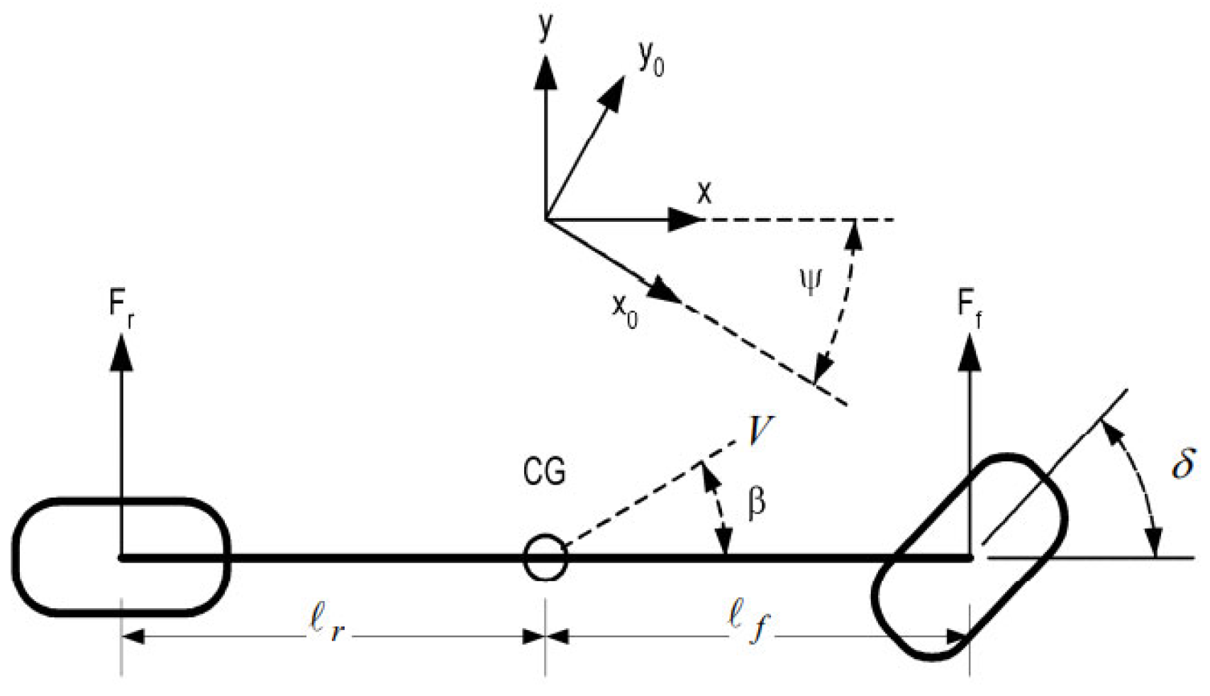
The lateral trajectory tracking controller utilizes a dynamic model of bicycle dynamics for lateral vehicle movement. The model has two degrees of freedom: side slip angle and the vehicle yaw angle, as illustrated in Figure 2, taken from [34]. This model is based on a well-known assumption that the vehicle longitudinal velocity is constant, which decouples the lateral dynamics from longitudinal dynamics to allow for a more focused study on the lateral behavior of the vehicle. Furthermore, it allows us to derive a Linear Time-Invariant (LTI) state space model, which is highly beneficial for control system design and analysis. If the velocity varies, the LTI model is replaced with an LPV (Linear Parameter Varying) model in which longitudinal velocity is a time-varying parameter.
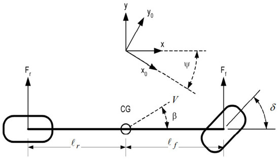
Figure 2.
Bicycle model for vehicle lateral dynamics.
The model can be described by the following two differential equations [34]:
where refers to the side slip angle, which is the angle formed between the vehicle’s longitudinal axis and the direction of the velocity vector at its center of gravity (CG); denotes the longitudinal speed of the vehicle, which is considered constant; is the vehicle’s heading angle; denotes the front wheel steering angle that controls the lateral dynamics of the vehicle. The term refers to the cornering stiffness at the front wheel, while denotes the same at the rear wheel; refers to the vehicle’s mass; denotes the vehicle’s moment of inertia; refers to the distance between the center of gravity and the front axle, and is the distance from center of gravity to the rear axle.
The state space representation of the model is given by
where is the state vector, and is the control input.
To use the bicycle model for trajectory tracking control, the error dynamics related to the reference trajectory are integrated into the model. The errors are treated as state variables, leading to a redefinition of the model by incorporating the errors as two extra states, as shown in Figure 3 below.
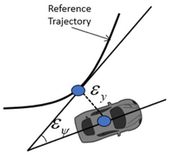
Figure 3.
Errors with respect to the reference trajectory.
In the above Figure, denotes the vehicle’s lateral deviation, which is defined as the lateral distance between the vehicle’s CG and the desired trajectory. Also, denotes the vehicle’s heading angle deviation, which is defined as the vehicle’s orientation error with respect to the reference trajectory.
The error dynamics of the vehicle’s heading angle are given by
With the vehicle traveling with constant velocity on a road with constant radius or slowly changing radius , it follows that the rate of change in the heading of the vehicle must equal the angular velocity of the vehicle, and since the angular velocity of the vehicle is , it follows that
Since the curvature of the road is , Equation (6) can be rewritten as
The lateral error dynamics are defined as
After incorporating the error dynamics, the resulting state space equation is
It is important to mention that the development of the dynamical bicycle model is based on the assumption that for small slip angles, the lateral forces are proportional to tire slip angle, and the proportionality constant is the cornering stiffness. Tire slip angle is defined as the angle between the orientation of the tire and the orientation of the velocity vector of the wheel, and it is a function of the side slip angle . The small slip angle range is between −4 and 4 degrees. As the slip angle increases beyond this range, we encounter a nonlinear region, as illustrated in Figure 4 (taken from the web), where the lateral forces depend not only on the slip angle but also on the normal tire load, tire road friction coefficient, and longitudinal tire force. In this situation, the bicycle model becomes invalid, and a more complicated tire model, incorporating the effect of these variables, is needed.
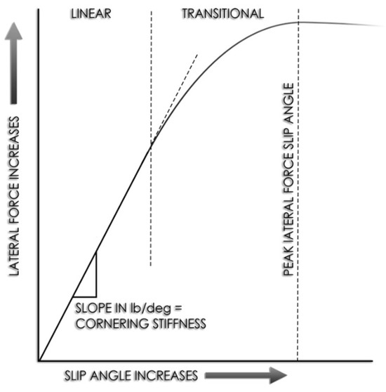
Figure 4.
Linear and nonlinear regions of the tire.
Due to the controller’s focus on operating within the tire’s linear region at small slip angles, we can overlook the slip angle when designing the feedback controller, allowing for a simplified model. However, the steady-state slip angle will still be utilized to compute the reference heading, as will be elaborated in the next section.
The simplified model is given by
2.2. Backstepping Controller Design
To design a backstepping controller for a system, it is essential for that system to be in the strict feedback form. The system described above was converted into the strict feedback form through a change in variables, as demonstrated below. If we substitute
We get a strict feedback form of the model as follows:
We are going to develop a backstepping controller for the transformed system (11) to regulate the lateral error and heading angle error, while following the road’s curvature.
Step 1: First, we use a stabilizing function to stabilize the first subsystem (lateral deviation error), as follows.
If we treat as the virtual control of the subsystem , we can find a stabilizing function which is the desired value of that will drive to zero, as .
Toward that goal, first, we introduce the following change in variables or error variables:
Taking the derivative of (12) yields,
Next, we choose the following Lyapunov function candidate to stabilize the error subsystem (14):
which yields the derivative
If in (16) (we will show in step 2 that ), then choosing with makes (16) negative definite and the origin globally asymptotically stable, achieving as .
Substituting in (14) and (16) yields, respectively,
Step 2: Next, our goal is to find a stabilizing function that will stabilize the second subsystem (heading angle deviation). If we treat (yaw rate) as the virtual control for the second subsystem , we can find its stabilizing function , as follows.
We define the third error variable as the difference between and its stabilizing function :
To proceed, we need to find the derivative of the second error variable in (13):
To stabilize the —error system, we choose the composite Lyapunov function candidate as
The derivative of which is given by
Clearly, if in (22) (we will prove that in step 3 below) and choosing to make the term with makes (22) negative definite. With that we have
Substituting (23) in (20) and (22) yields, respectively,
The error system given by (17) and (24) can be expressed as
where is a skew-symmetric Hurwitz matrix rendering and asymptotically for .
Step 3: Next, our goal is to stabilize the complete system using a backstepping control law . To do that, first, we find the derivative of (19) as
Then, we choose a composite Lyapunov function candidate to stabilize the —error system as
Taking the derivative of (28) yields
Choosing to be the backstepping control law that makes the term in (29) yields
Substituting (30) in (27) and (29), respectively, yields
From Equations (28) and (32), the global uniform boundness of and is ensured by the Lasalle–Yoshizawa theorem (which is stated below), and it can be concluded that as . In view of this, is bounded since and it can be concluded that . Furthermore, the boundedness of follows from the boundness of and , since . Also, the boundness of follows from the boundness of and , since . In view of the above, it can be concluded that in (30) is also bounded.
Lasalle–Yoshizawa Theorem [1]:
Let be an equilibrium point of . Let be a continuously differentiable function such that
where is a continuous function. Then, all solutions of are globally uniformly bounded and satisfy . In addition, if is positive definite then the equilibrium is globally uniformly asymptotically stable (GUAS).
The complete error system given by (17), (24), and (31) can be expressed as
where is a skew-symmetric Hurwitz matrix for all rendering , and asymptotically, and is bounded.
Step 4: Converting the state space equation from the z-domain to the x-domain
Substituting (24) in (35) yields
Substituting (19) in (36) yields
Substituting (23) in (37) yields
Substituting (31) in (39) yields
Taking the derivative of (23) yields
Substituting (41) in (40) yields
Combining (34), (38), and (42), we obtain the same system in (11) combined with the derived backstepping control law , as follows:
The next step is to find the backstepping control law in the x-domain and substitute it in (43).
Substituting (12) and (13) in (23) with and yields
Taking the derivative of (44) yields
Substituting (13), (19) and (45) in (30) yields
Substituting (46) in (43) yields the closed-loop system:
The parameters are design parameters, also known as the Lyapunov coefficients, the choice of which significantly affects the controller performance. These parameters can be tuned to introduce damping and improve the tracking and regulation performance of the controller.
2.3. Dynamic Feedforward and Reference Heading Derivation
To effectively navigate curved roads, curvature compensation is essential. We must determine the required steering wheel angle for safely executing a turn with a radius of R. Utilizing the bicycle model (3), we can calculate both the steering wheel angle and the side slip angle during steady-state cornering, assuming the vehicle maintains a constant speed on a curve of consistent radius R.
When all derivative terms die out and substituting in (3) by , we have
As can be seen, since the vehicle speed and the road curvature are known, from Equation (48), we can solve two unknowns, and . After solving them, we obtain
Since represents the steering angle needed to navigate a curve , it will be incorporated into the feedback control law to adjust for the road’s curvature.
The steady state side slip angle, denoted as , serves as the vehicle’s reference heading. During steady state cornering, where both the road radius and vehicle speed remain constant, the slip angles of the tires are fully established, leading to an automatically determined side slip angle for the vehicle. This is further illustrated by examining the dynamics of lateral error, as given by
Since becomes zero at the steady state, we get
Thus, the steady state side slip angle of the vehicle is given by
This means that we do not aim for the heading angle error to be zero; instead, we want it to match the steady state side slip angle. Therefore, we require that .
3. Results
3.1. Simulation Results
A signal generator was employed to create a simulated route for the vehicle at varying speeds and different curvature values. To attain the desired response, the Lyapunov coefficients were tuned. The coefficient was tuned to minimize steady state error; was adjusted to introduce damping for the errors, and was tuned to enhance vehicle stability by controlling the yaw rate to avoid excessive steering. Tuning these parameters is a trial-and-error process. A recommended approach is to initially set all of them to 1 and observe the system’s response. Then, modify them accordingly, one at a time, to understand the effect of each. For instance, if there is a steady state error, start by adjusting . If the system is over- or under-damped, start by adjusting If there are oscillations or excessive steering, start by adjusting .
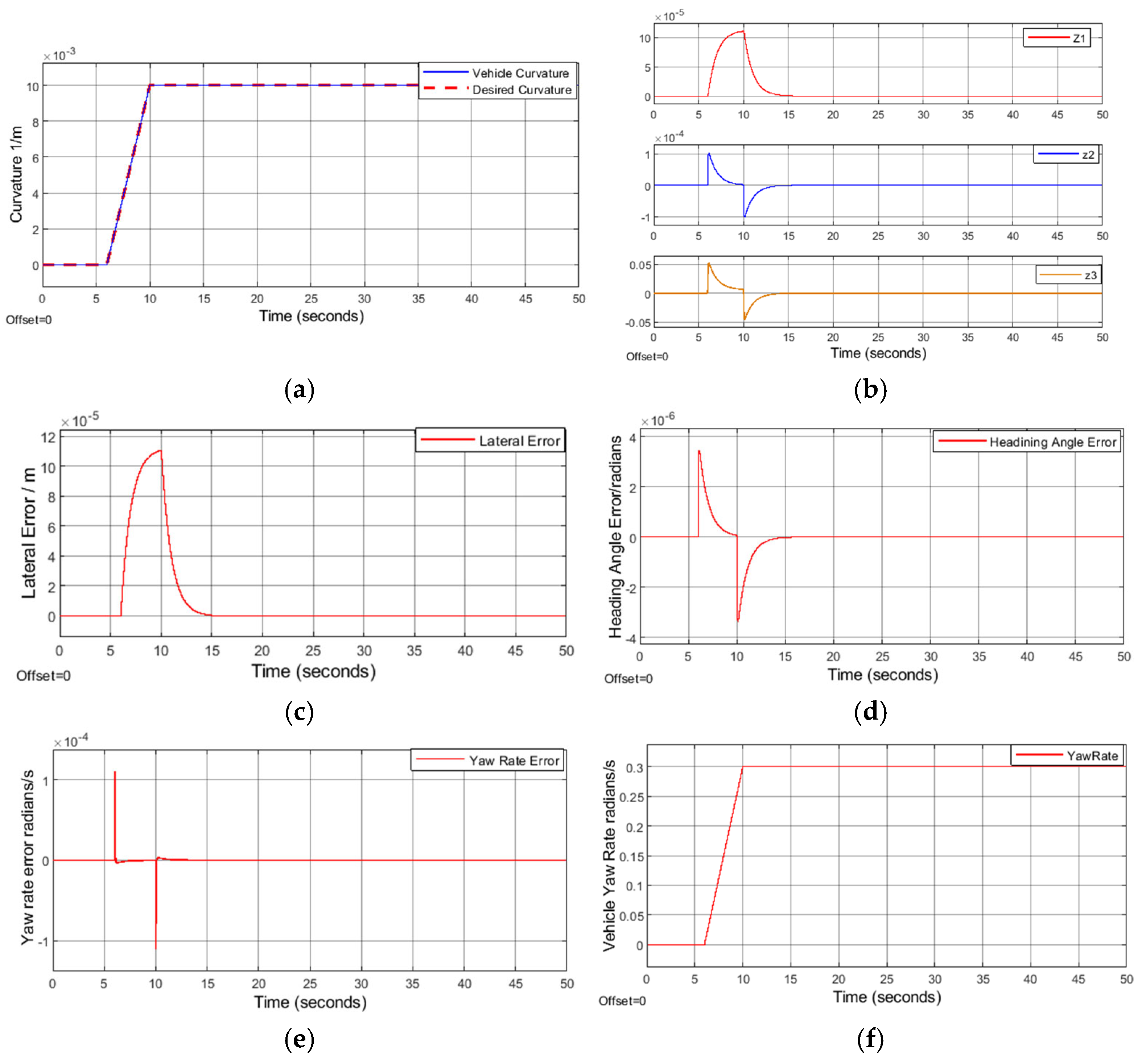
Different trajectories were generated to emulate different driving scenarios. In Figure 5a–f below, the trajectory starts with zero curvature and then ramps up to a constant radius curve of 100 m at 30 mps/108 kph to emulate transitioning from a straight road to a curved road. Figure 5a illustrates the vehicle’s actual curvature following the desired curvature very well. Figure 5b–e illustrates the virtual control errors, lateral position error, heading angle error, and yaw rate error, respectively. In the transitioning period from 6 to 10 s, there were some dynamics in the errors, and then, they all converged to zero asymptotically at steady state, as we proved in Section 2 above using the Lassalle–Yoshizawa theorem. Figure 5f illustrates the vehicle yaw rate during the maneuver, which indicates vehicle stability.
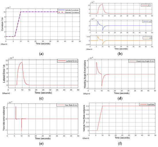
Figure 5.
30 mps/108 kph, 100m radius curve, (a) Measured vehicle curvature vs. desired curvature. (b) Virtual control errors. (c) Lateral position error. (d) Heading angle error. (e) Yaw rate error. (f) Vehicle yaw rate.
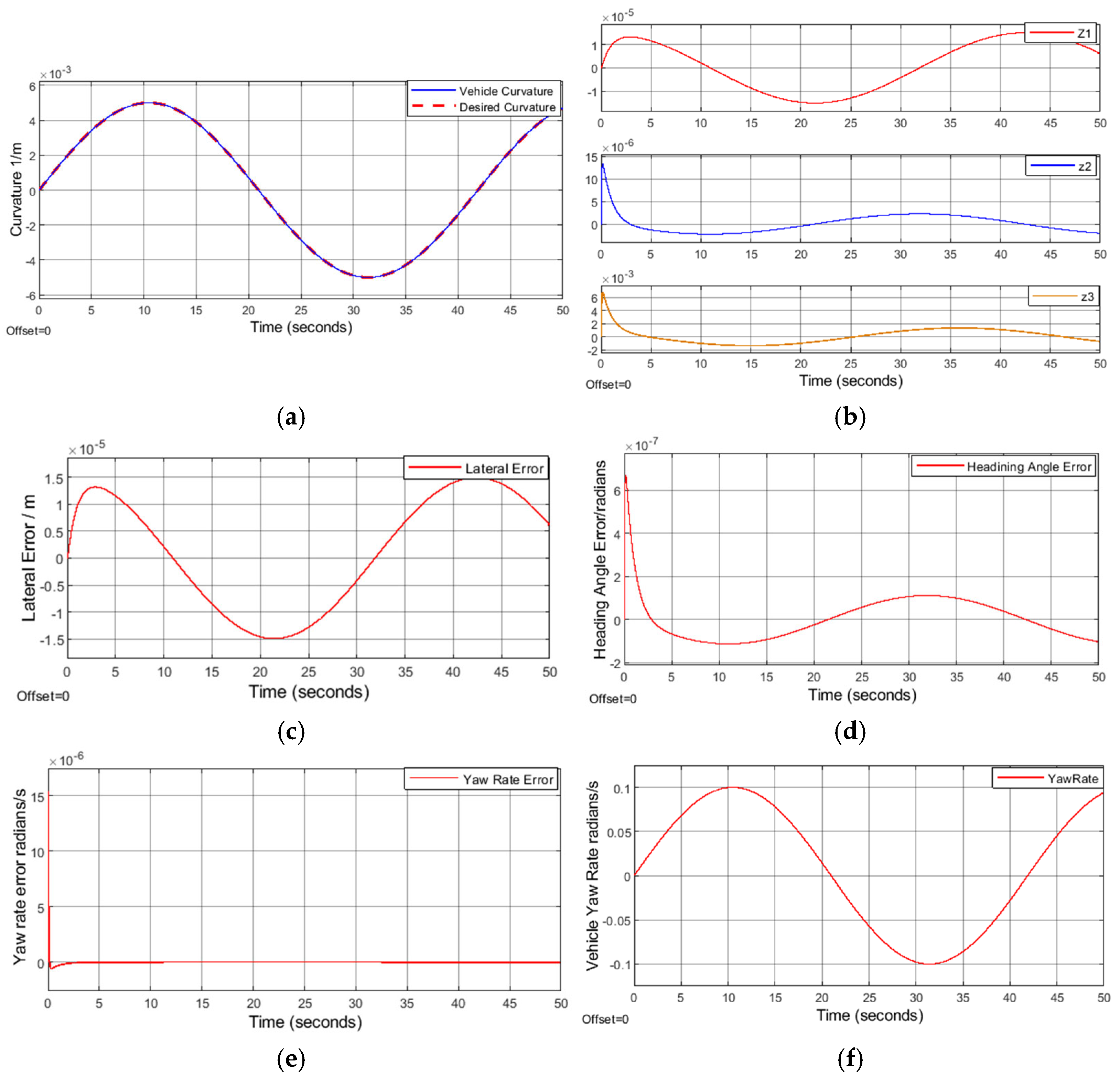
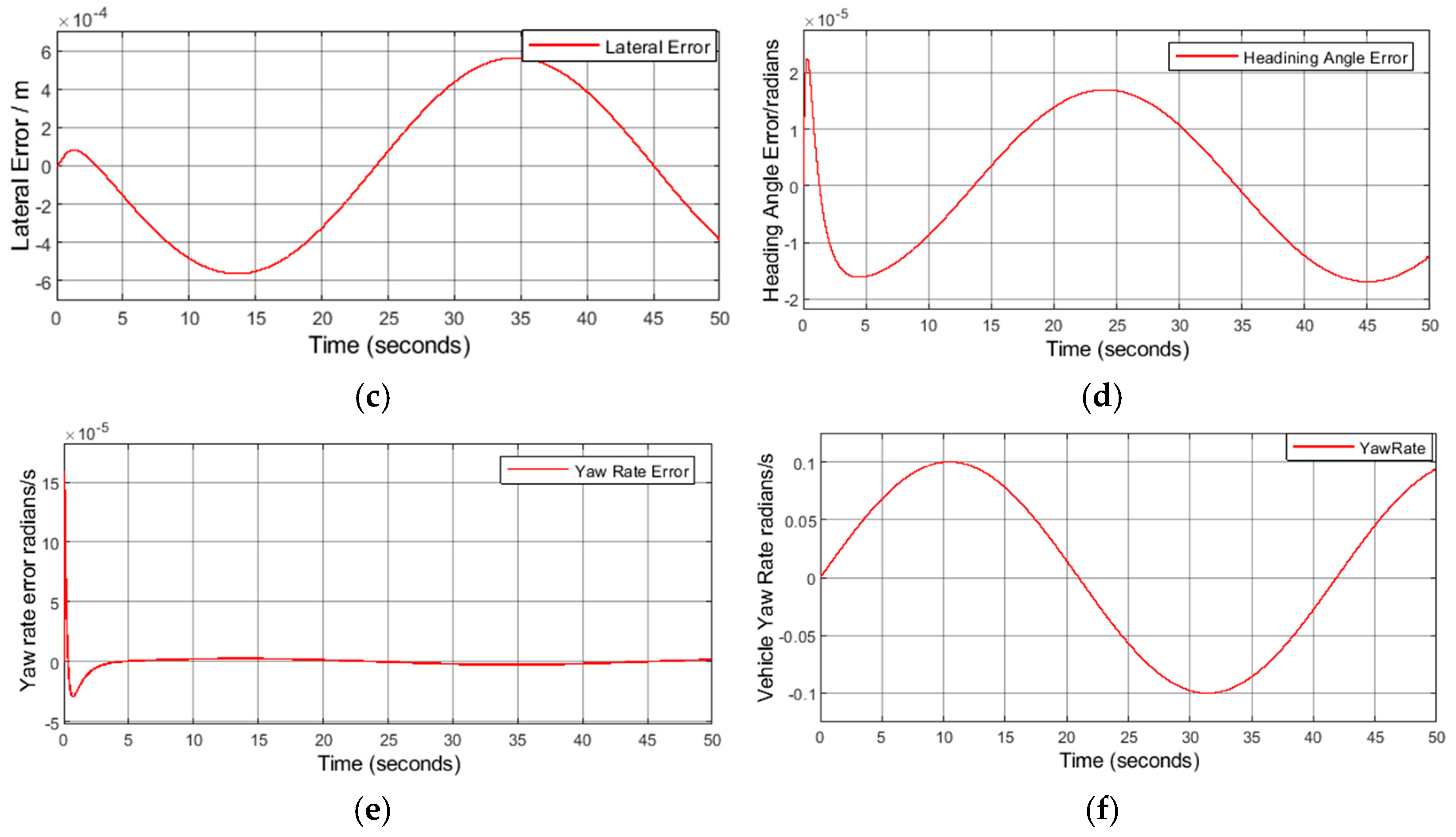
In Figure 6a–f below, a sine wave path was generated at 20 mps/72 kph to emulate successive curves in different directions or successive lane changes. The sine wave amplitude is 0.005 to represent a road of 200 m radius. Figure 6a illustrates the vehicle’s actual curvature following the desired curvature with near-zero errors. Figure 6b–e illustrates the virtual control errors, lateral position error, heading angle error, and yaw rate error, respectively. In this case, because the desired curvature is continuously changing and does not go to a steady-state value, the errors are also continuously changing to keep up with the changing curvature request. Figure 6f illustrates the vehicle yaw rate during the maneuver.
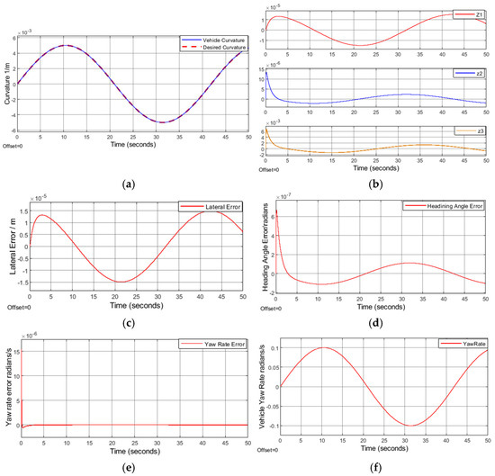
Figure 6.
20 mps/72 kph, 200 m radius curve, . (a) Measured vehicle curvature vs. desired curvature. (b) Virtual control errors. (c) Lateral position error (d) Heading angle error. (e) Yaw rate error. (f) Vehicle yaw rate.
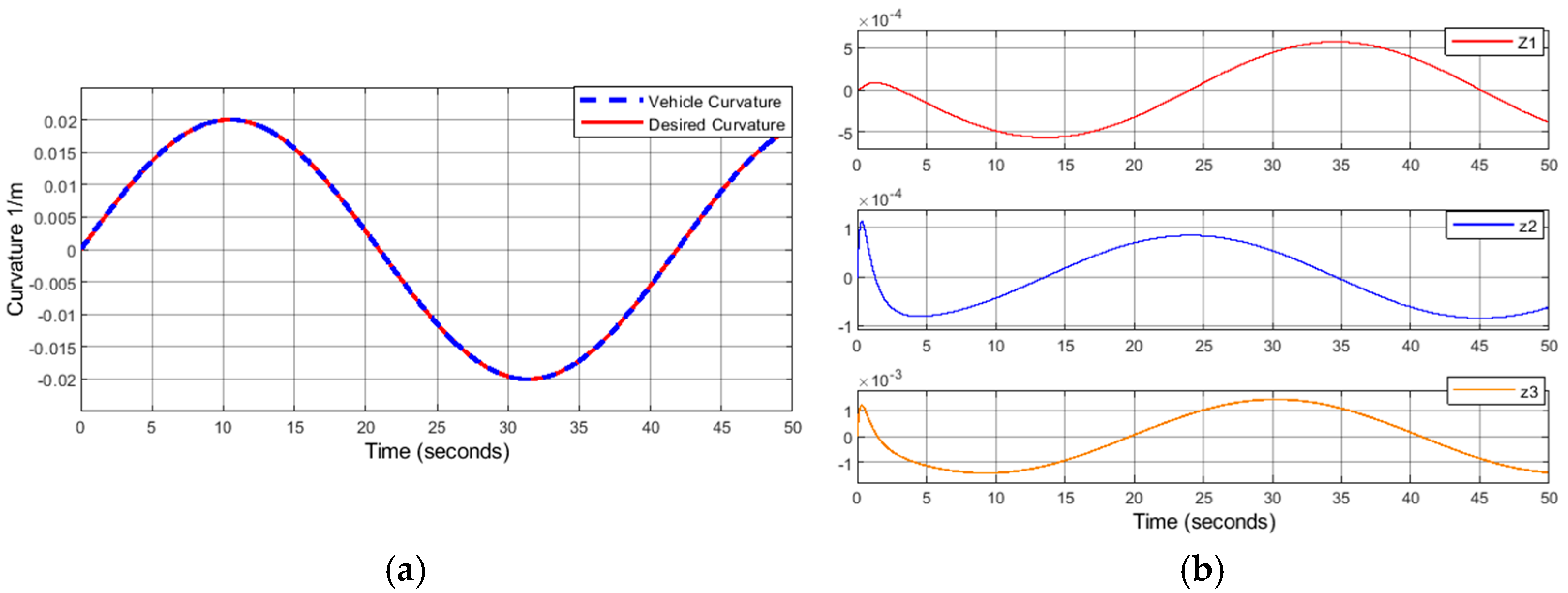
The rest of the figures show the controller response to very low speeds (5 mps/18 kph) and below. Even though such speeds are not highway speeds, they can be encountered at traffic jam situations and stop-and-go scenarios in urban traffic. Figure 7a–f below demonstrates the response to a sinewave at a sharper curve (50 m radius) and low speed 5 mps/18 kph, which still shows a tracking trajectory with near-zero errors. At speeds lower than 5 mps/18 kph, a very poor controller response was noticed, and the same control gains that worked for speeds higher than 5 mps/18 kph did not work. Higher controller gains are needed for such low speeds.
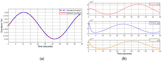
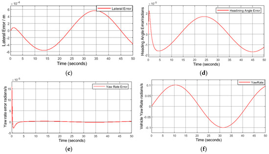
Figure 7.
5 mps/18 kph, 50 m radius curve, . (a) Measured vehicle curvature vs. desired curvature. (b) Virtual control errors. (c) Lateral position error (d) Heading angle error. (e) Yaw rate error. (f) Vehicle yaw rate.
Figure 8a,b below illustrates the response to a 100 m radius curve at 2 mps/7.2 kph with two different sets of control gains, and respectively. As can be seen, better response is shown in Figure 8b with higher control gains.

Figure 8.
Measured vehicle curvature vs. desired curvature at 2 mps/7.2 kph, 100 m radius curve. (a) . (b) .
Figure 9a,b below illustrates the response to a 100 m radius curve at 1 mps/3.6 kph with two different sets of control gains. A very poor response is noticed in Figure 9a with the same original high-speed gains ). Changing the controller gains from to improved the response, as can be seen in Figure 9b.

Figure 9.
Measured vehicle curvature vs. desired curvature at 1 mps/3.6 kph, 100 m radius curve. (a) . (b) .
At speeds of 0.6 mps/2.16 kph and below, oscillations are noticed regardless of the choice of the control parameters, as can be seen in Figure 10a,b. The reason is due to the derivation of both the feedback controller and the feedforward based on the dynamic bicycle model, which depends on lateral forces, yaw rate, and side slip angle. At such low speeds (0.6 mps/2.16 kph), there are not enough lateral forces to generate a slip angle, and the yaw rate is a very small, noisy signal. For this reason, we should switch to a kinematic vehicle model at such low speeds, which does not consider lateral forces and only depends on geometrical relationships. It is very important to mention that switching to the kinematic model should only happen at very low speeds (0.6 mps/2.16 kph and below) because it does not work at high speeds when lateral forces start to develop.

Figure 10.
0.6 mps/2.16 kph and below, 100 m radius curve. Similar response regardless of the values of . (a) Measured vehicle curvature vs. desired curvature. (b) Vehicle yaw rate.
3.2. Experimental Results
Experiments were conducted on a prototype vehicle to validate the backstepping trajectory tracking controller in both a private test track and a public highway. The vehicle is equipped with dSPACE AutoBox, a rapid control prototyping (RCP), and data logging system that replaces an electronic control unit (ECU). This allows developers to test and tune control functions developed using model-based design in MATLAB/Simulink. The vehicle is also equipped with a forward-facing camera (Mobileye in the prototype vehicle is used), which is a core component for automatic steering systems, such as trajectory tracking. The camera uses computer vision and deep learning techniques to detect and interpret lane markings, including solid lines, dotted lines, yellow lines, curbs, and other road boundaries. It measures the distance from the vehicle to the detected lane markings and the curvature of the road. A planning algorithm then uses the camera data to generate a safe trajectory for the vehicle to follow in the center of the lane and send it to the trajectory tracking controller. The vehicle is also equipped with a robot operating system (ROS) that hosts the camera data processing and planning algorithm, while our control algorithm is in the dSPASE AutoBox, which communicates with the ROS system via Ethernet. The vehicle is also equipped with electric power steering (EPS) to actuate steering, in addition to other basic sensors such as an inertial measurement unit (IMU), a steering angle sensor, and a wheel speed sensor. The dSPASE AutoBox communicates with the EPS and other sensors via control area network (CAN).
The Figures below show a 700 s/11 min recording with multiple scenarios on a public highway with the vehicle driven at approximately 31 mps/122 kph. This covers a significant distance with various scenarios, including straight roads, curved roads with different radii, and lane changes. Figure 11a depicts the desired road curvature coming from the camera versus the vehicle’s actual curvature, which illustrates that the vehicle curvature is following the desired curvature very well. Figure 11b is a zoomed-in view of Figure 11a, illustrating a section that transitions from a straight road to a mild curve (approximately 0.0005 ), then back to a straight road section, followed by a sharper curve (approximately 0.002 ), and finally, exiting to another straight section. As illustrated in Figure 11b, the controller’s behavior at curve entry and curve exit is very good, which are the most challenging scenarios due to the transitioning maneuver. Figure 11c,d illustrates the lateral position error and the heading angle error throughout the entire recording. As the recording encompasses a range of scenarios and transition maneuvers, the errors are not constant and will fluctuate with each maneuver. The spikes in errors align with changes in maneuvers (such as entering or exiting a curve), as these correspond to a shift in the controller’s setpoint. It can be noticed by examining Figure 11c, for example, that the lateral error is very small on a straight road (below 0.15 m), and it increases up to 0.4 m at curves and lane changes. This is because on a straight road, there is only feedback steering angle and no feed forward, but at curves and lane changes, a feedforward is added to the feedback; that is why the lateral error increases, but that does not mean that we are not following the trajectory closely, as can be seen from Figure 11a. Likewise, in Figure 11d, the heading angle error is larger at curves and lane change maneuvers because of the addition of the feedforward, and again, we are still following the trajectory very well, as can be seen in Figure 11a. Figure 11e is a zoomed-in view of Figure 11c, focusing on the lateral position error during a straight section, while Figure 11f is a zoomed-in view of Figure 11d, focusing on the heading angle error during the same straight section. As evident, the peak lateral position error is approximately 0.12 m and the peak heading angle error is approximately 0.0022 radians, which is excellent and not easily achieved by a real vehicle on the road. Figure 11g illustrates the desired steering angle commanded from the controller vs. the vehicle’s actual measured angle along the entire recording. As can be seen, the controller is able to obtain the desired angle it is requesting with near-zero error without saturating the actuator, even though there are high actuator limitations at such high speed.
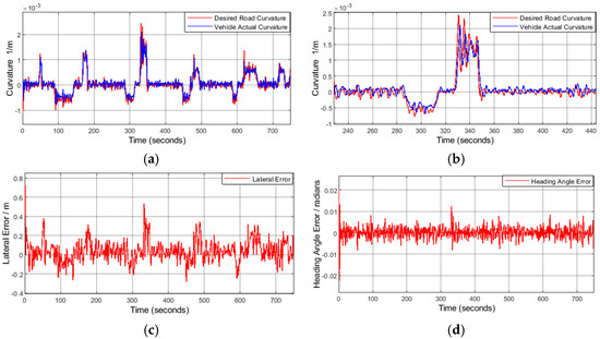
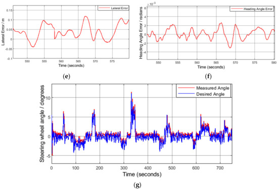
Figure 11.
(a) Vehicle’s actual curvature vs. desired road curvature in multiple scenarios of straight, sharp curves, mild curves, and lane changes at about 31 mps/122 kph (b) A zoomed-in figure from the previous one demonstrating transitioning from straight to curved road and vice versa. (c) Lateral position error. (d) Heading angle error. (e) Zoomed-in view of lateral position error in a straight road section. (f) Zoomed-in view of heading angle error in a straight road section. (g) Desired steering angle commanded from the controller vs. vehicle’s actual measured steering angle.
4. Discussion
The performance of the developed method was validated both in simulations and experimentally. Simulation validations were used as an initial proof of concept for the method under ideal conditions, including an ideal vehicle model and steering model, an ideal actuator, ideal sensors, and the absence of environmental disturbances. The Simulations were conducted at a speed range of 1 kph–108 kph. It was observed that the controller performed very well at speeds above 5 mps/18 kph and was able to drive the steady state virtual control errors () and the actual errors (lateral position error, heading angle error, and yaw rate error) to zero, as was proven in Section 2, but as the speed decreases below 5 mps/18 kph, the performance degrades gradually with decreasing speed. Nevertheless, we were able to improve it with different control gains, which suggests the creation of gain scheduling for the controller gains (, ) as a function of speed. We were able to retune the controller gains for a better performance until we reached 0.6 mps/2.16 kph, at which point, the performance was very poor and unstable regardless of the controller gains. The poor performance at such low speeds should not be ignored, as it can be encountered at traffic jams. This issue is not due to the control method but rather to the model used in the controller, which is the dynamic bicycle model. This model is derived based on lateral forces and slip angle, which are very small at very low speeds, making it inaccurate at such speeds. This problem can be solved by switching to a kinematic model only at very low speeds. It is crucial to note that the kinematic model is only applicable at very low speeds and cannot be used at higher speeds, as previously mentioned, because it disregards the lateral forces that increase at higher speeds.
Experimental results were conducted in a prototype vehicle on a public highway to validate the proposed method in the real-world environment, where a layer of complexity is added due to imperfect sensors and actuators, unmodeled vehicle dynamics, actuators, communication delays, and external disturbances. Due to these factors, the controller response will not be the same as in the case of the ideal simulation environment, and the errors cannot be driven exactly to zero. For example, the trajectory is generated using camera data, and since the camera data is noisy, the trajectory will be noisy. Since the controller is designed to closely track the trajectory, we notice the same noise in the error and trajectory plots. However, this noise is hardly felt in the car and can be mitigated with further processing of the trajectory signals. Additionally, the trajectory generated from the camera may have a bias relative to the lane lines, meaning that it will not be centered in the lane. Since our goal is to keep the vehicle in the center of the lane, we tune the controller to deviate from the trajectory to compensate for this bias, resulting in a non-zero error, even though we are centered in the lane.
5. Conclusions
In this paper, an autonomous lateral trajectory tracking controller is designed using the backstepping control method based on the dynamic bicycle model. It is proven using Lyapunov stability theory and the Lassalle–Yoshizawa theorem that the developed controller successfully achieves both asymptotic stability of the errors and excellent tracking of the desired trajectory. A dynamic feedforward compensator was derived to compute the steering angle required to negotiate a curve, also based on the dynamic bicycle model. The dynamic feedforward was able to drive the vehicle to follow the road curve with excellent curve entry and curve exit performance. Both simulation and experimental results demonstrated the effectiveness of the developed method. However, a limitation of the developed method is that it does not function at very low speeds (below 2.16 kph). This limitation is not due to the control method used but rather to the vehicle model employed in the controller, which is the dynamic bicycle model. This model depends on the vehicle’s lateral forces, and lateral forces are negligible at such low speeds. To address this issue, we should switch to a kinematic model only at such low speeds and derive both the backstepping control law and the feedforward based on it, as kinematic models ignore vehicle forces and rely solely on geometrical relationships.
Another point we would like to mention is that the controller was designed based on the assumption that the bicycle model parameters (cornering stiffness, vehicle mass, moment of inertia, and center of gravity) are known and constant. However, these parameters are not actually constant and can vary significantly in road vehicles, affecting the control performance. Adaptive backstepping, which assumes these parameters to be unknown and develops adaptive laws to estimate them online, is currently under investigation for a future paper.
Author Contributions
Conceptualization, L.K., M.D. and L.K.; Software, L.K.; Validation, L.K.; Formal analysis, L.K.; Investigation, L.K.; Resources, L.K.; Writing—original draft, L.K.; Writing—review & editing, M.D.; Visualization, M.D.; Supervision, M.D.; Project administration, M.D. All authors have read and agreed to the published version of the manuscript.
Funding
This research received no external funding.
Data Availability Statement
The data presented in this study are available on request from the corresponding author.
Conflicts of Interest
There are no conflicts of interest.
References
- Khasawneh, L.; Das, M. A Robust Electric Power-Steering-Angle Controller for Autonomous Vehicles with Disturbance Rejection. Electronics 2022, 11, 1337. [Google Scholar] [CrossRef]
- Krstic, M.; Kanellakopoulos, I.; Kokotovic, P.V. State Feedback. In Nonlinear and Adaptive Control Design; Wiley: New York, NY, USA, 1995; pp. 29–84. [Google Scholar]
- Wang, W.; Zhou, J.; Wen, C.; Long, J. Adaptive Backstepping Control of Uncertain Nonlinear Systems with Input and State Quantization. IEEE Trans. Autom. Control 2022, 67, 6754–6761. [Google Scholar] [CrossRef]
- Xu, Z.; Yang, S.X.; Gadsden, S.A. Enhanced Bioinspired Backstepping Control for a Mobile Robot with Unscented Kalman Filter. IEEE Access 2020, 8, 125899–125908. [Google Scholar] [CrossRef]
- Sehgal, K.; Upadhyaya, S.; Keshav; Verma, M.; Rayguru, M.M. Backstepping based Trajectory Tracking Control of a Class of Reconfigurable Mobile Robot. In Proceedings of the 2021 3rd International Conference on Advances in Computing, Communication Control and Networking (ICAC3N), Greater Noida, India, 17–18 December 2021; pp. 752–756. [Google Scholar] [CrossRef]
- Dierks, T.; Jagannathan, S. Control of Nonholonomic Mobile Robot Formations: Backstepping Kinematics into Dynamics. In Proceedings of the 2007 IEEE International Conference on Control Applications, Singapore, 1–3 October 2007; pp. 94–99. [Google Scholar] [CrossRef]
- Shen, C.; Shi, Y.; Buckham, B. Trajectory Tracking Control of an Autonomous Underwater Vehicle Using Lyapunov-Based Model Predictive Control. IEEE Trans. Ind. Electron. 2018, 65, 5796–5805. [Google Scholar] [CrossRef]
- Sun, B.; Zhu, D.; Yang, S.X. A Bioinspired Filtered Backstepping Tracking Control of 7000-m Manned Submarine Vehicle. IEEE Trans. Ind. Electron. 2014, 61, 3682–3693. [Google Scholar] [CrossRef]
- Aguiar, A.P.; Hespanha, J.P. Trajectory-Tracking and Path-Following of Underactuated Autonomous Vehicles with Parametric Modeling Uncertainty. IEEE Trans. Autom. Control 2007, 52, 1362–1379. [Google Scholar] [CrossRef]
- Ao, D.; Huang, W.; Wong, P.K.; Li, J. Robust Backstepping Super-Twisting Sliding Mode Control for Autonomous Vehicle Path Following. IEEE Access 2021, 9, 123165–123177. [Google Scholar] [CrossRef]
- Hu, C.; Wang, Z.; Taghavifar, H.; Na, J.; Qin, Y.; Guo, J.; Wei, C. MME-EKF-Based Path-Tracking Control of Autonomous Vehicles Considering Input Saturation. IEEE Trans. Veh. Technol. 2019, 68, 5246–5259. [Google Scholar] [CrossRef]
- Chen, J.; Shuai, Z.; Zhang, H.; Zhao, W. Path Following Control of Autonomous Four-Wheel-Independent-Drive Electric Vehicles via Second-Order Sliding Mode and Nonlinear Disturbance Observer Techniques. IEEE Trans. Ind. Electron. 2021, 68, 2460–2469. [Google Scholar] [CrossRef]
- Wu, Y.; Wang, L.; Zhang, J.; Li, F. Path Following Control of Autonomous Ground Vehicle Based on Nonsingular Terminal Sliding Mode and Active Disturbance Rejection Control. IEEE Trans. Veh. Technol. 2019, 68, 6379–6390. [Google Scholar] [CrossRef]
- Thrun, S.; Montemerlo, M.; Dahlkamp, H.; Stavens, D.; Aron, A.; Diebel, J.; Fong, P.; Gale, J.; Halpenny, M.; Hoffmann, G.; et al. Stanley: The robot that won the DARPA grand challenge. J. Field Robot. 2006, 23, 661–692. [Google Scholar] [CrossRef]
- Hoffmann, G.M.; Tomlin, C.J.; Montemerlo, M.; Thrun, S. Autonomous Automobile Trajectory Tracking for Off-Road Driving: Controller Design, Experimental Validation and Racing. In Proceedings of the 2007 American Control Conference, New York, NY, USA, 9–13 July 2007; pp. 2296–2301. [Google Scholar] [CrossRef]
- Amidi, O.; Thorpe, C.E. Integrated mobile robot control. Mob. Robot. 1991, 1388, 504–524. [Google Scholar] [CrossRef]
- Park, M.; Lee, S.; Han, W. Development of lateral control system for autonomous vehicle based on adaptive pure pursuit algorithm. In Proceedings of the 2014 14th International Conference on Control, Automation and Systems (ICCAS 2014), Goyang, Republic of Korea, 22–25 October 2014; pp. 1443–1447. [Google Scholar] [CrossRef]
- Elbanhawi, M.; Simic, M.; Jazar, R. Receding horizon lateral vehicle control for pure pursuit path tracking. J. Vib. Control 2018, 24, 619–642. [Google Scholar] [CrossRef]
- Guo, H.; Cao, D.; Chen, H.; Sun, Z.; Hu, Y. Model predictive path following control for autonomous cars considering a measurable disturbance: Implementation, testing, and verification. Mech. Syst. Signal Process. 2019, 118, 41–60. [Google Scholar] [CrossRef]
- Cui, Q.; Ding, R.; Zhou, B.; Wu, X. Path-tracking of an autonomous vehicle via model predictive control and nonlinear filtering. Proc. Inst. Mech. Eng. Part D J. Automob. Eng. 2017, 232, 1237–1252. [Google Scholar] [CrossRef]
- Ji, J.; Khajepour, A.; Melek, W.W.; Huang, Y. Path Planning and Tracking for Vehicle Collision Avoidance Based on Model Predictive Control with Multiconstraints. IEEE Trans. Veh. Technol. 2017, 66, 952–964. [Google Scholar] [CrossRef]
- Huang, Y.; Ding, H.; Zhang, Y.; Wang, H.; Cao, D.; Xu, N.; Hu, C. A Motion Planning and Tracking Framework for Autonomous Vehicles Based on Artificial Potential Field Elaborated Resistance Network Approach. IEEE Trans. Ind. Electron. 2020, 67, 1376–1386. [Google Scholar] [CrossRef]
- Chu, D.; Li, H.; Zhao, C.; Zhou, T. Trajectory Tracking of Autonomous Vehicle Based on Model Predictive Control with PID Feedback. IEEE Trans. Intell. Transp. Syst. 2023, 24, 2239–2250. [Google Scholar] [CrossRef]
- Funke, J.; Brown, M.; Erlien, S.M.; Gerdes, J.C. Collision Avoidance and Stabilization for Autonomous Vehicles in Emergency Scenarios. IEEE Trans. Control Syst. Technol. 2017, 25, 1204–1216. [Google Scholar] [CrossRef]
- Marino, R.; Scalzi, S.; Netto, M. Nested PID steering control for lane keeping in autonomous vehicles. Control Eng. Pract. 2011, 19, 1459–1467. [Google Scholar] [CrossRef]
- Valiente, R.; Zaman, M.; Ozer, S.; Fallah, Y.P. Controlling Steering Angle for Cooperative Self-driving Vehicles utilizing CNN and LSTM-based Deep Networks. In Proceedings of the 2019 IEEE Intelligent Vehicles Symposium (IV), Paris, France, 9–12 June 2019; pp. 2423–2428. [Google Scholar] [CrossRef]
- Umamaheswari, V.; Amarjyoti, S.; Bakshi, T.; Singh, A. Steering angle estimation for autonomous vehicle navigation using hough and Euclidean transform. In Proceedings of the 2015 IEEE International Conference on Signal Processing, Informatics, Communication and Energy Systems (SPICES), Kozhikode, India, 19–21 February 2015; pp. 1–5. [Google Scholar] [CrossRef]
- Ranjith Rochan, M.; Aarthi Alagammai, K.; Sujatha, J. Computer Vision Based Novel Steering Angle Calculation for Autonomous Vehicles. In Proceedings of the 2018 Second IEEE International Conference on Robotic Computing (IRC), Laguna Hills, CA, USA, 31 January–2 February 2018; pp. 143–146. [Google Scholar] [CrossRef]
- Eraqi, H.M.; Moustafa, M.N.; Honer, J. End-to-end deep learning for steering autonomous vehicles considering temporal dependencies. In Proceedings of the 31st Conference on Neural Information Processing Systems (NIPS), Machine Learning for Intelligent Transportation Systems Workshop, Long Beach, CA, USA, 4–9 December 2017. [Google Scholar]
- Lee, K.; Jeon, S.; Kim, H.; Kum, D. Optimal Path Tracking Control of Autonomous Vehicle: Adaptive Full-State Linear Quadratic Gaussian (LQG) Control. IEEE Access 2019, 7, 109120–109133. [Google Scholar] [CrossRef]
- Zhou, X.; Wang, Z.; Shen, H.; Wang, J. Robust Adaptive Path-Tracking Control of Autonomous Ground Vehicles with Considerations of Steering System Backlash. IEEE Trans. Intell. Veh. 2022, 7, 315–325. [Google Scholar] [CrossRef]
- Xu, S.; Peng, H. Design, Analysis, and Experiments of Preview Path Tracking Control for Autonomous Vehicles. IEEE Trans. Intell. Transp. Syst. 2020, 21, 48–58. [Google Scholar] [CrossRef]
- Khasawneh, L.; Das, M. Lateral Trajectory Tracking Control using Backstepping Method for Autonomous Vehicles. In Proceedings of the 2021 64th IEEE International Midwest Symposium Conference on Circuits and Systems, Lansing, MI, USA, 9–11 August 2021. [Google Scholar]
- Rajamani, R. Lateral Vehicle Dynamics. In Vehicle Dynamics and Control, 2nd ed.; Springer: New York, NY, USA; Dordrecht, The Netherlands; Berlin/Heidelberg, Germany; London, UK, 2012; p. 38. [Google Scholar]
Disclaimer/Publisher’s Note: The statements, opinions and data contained in all publications are solely those of the individual author(s) and contributor(s) and not of MDPI and/or the editor(s). MDPI and/or the editor(s) disclaim responsibility for any injury to people or property resulting from any ideas, methods, instructions or products referred to in the content. |
© 2025 by the authors. Licensee MDPI, Basel, Switzerland. This article is an open access article distributed under the terms and conditions of the Creative Commons Attribution (CC BY) license (https://creativecommons.org/licenses/by/4.0/).


