An Improved Adaptive Car-Following Model Based on the Unscented Kalman Filter for Vehicle Platoons’ Speed Control

Abstract

This study proposes an adaptive car-following model based on the unscented Kalman filter algorithm to enable coordinated speed control in vehicle platoons and to address key limitations present in conventional car-following models. Traditional models generally assume a fixed maximum speed within the optimal velocity function, which constrains effective platoon speed regulation across road segments with varying speed limits and lacks adaptability to dynamic scenarios such as changes in the platoon leader’s speed or substitution of the lead vehicle. The proposed adaptive model utilizes state estimation based on the unscented Kalman filter to dynamically identify each vehicle’s maximum achievable speed and to adjust inter-vehicle constraints, thereby enforcing a unified speed reference across the platoon. By estimating these maximum speeds and transmitting them to individual follower vehicles via vehicle-to-vehicle communication, the model promotes smooth acceleration and deceleration behavior, reduces headway variability, and mitigates shockwave propagation within the platoon. Simulation studies—covering both single-leader acceleration and intermittent acceleration scenarios—demonstrate that, compared with conventional car-following models, the adaptive model based on the unscented Kalman filter achieves superior speed synchronization, improved headway stability, and smoother acceleration transitions. These enhancements lead to substantial improvements in traffic flow efficiency and string stability. The proposed approach offers a practical solution for coordinated platoon speed control in intelligent transportation systems, with promising application prospects for real-world implementation.

1. Introduction

Accurate and coordinated determination of vehicle speeds within platoons is a crucial technology underpinning successful platoon control. Effective platoon management relies fundamentally on precise speed control, which directly influences platoon stability, headway management, and overall traffic efficiency [1,2]. Early platoon studies have demonstrated that inconsistent speed assignments among vehicles frequently result in amplified disturbances, causing undesirable oscillations, reduced throughput, and increased safety risks. To mitigate these issues, researchers have proposed various strategies to synchronize platoon speeds, including optimal velocity-based car-following models (CFMs) that assign speeds dynamically according to headway conditions [3,4,5]. With advances in connected vehicle technologies, cooperative speed control strategies leveraging vehicle-to-vehicle (V2V) communication have emerged, enabling vehicles within a platoon to share speed and acceleration data in real time, thus, significantly enhancing platoon string stability and speed synchronization.

The car-following model (CFM) is a widely adopted framework for characterizing how drivers adjust their speed in response to the preceding vehicle, primarily to ensure safety and enhance traffic efficiency. In CFMs, the optimal speed of the following vehicle is typically determined by the headway to the vehicle ahead, with the optimal velocity function (OVF) serving as the cornerstone of many model variants. Several classical car-following models have established the theoretical foundation for modern traffic flow research. Among them, the General Motors (GM) model, as one of the earliest microscopic traffic models, introduced a linear relationship between the follower’s acceleration and the relative speed and spacing to the leader, thereby providing a basis for subsequent developments. Bando et al. [6] first proposed the OVF based on a hyperbolic tangent function and established the optimal velocity model (OVM), which emphasizes the nonlinear relationship between headway and optimal speed. Helbing and Tilch [7] further refined the OVM by incorporating negative speed differences and vehicle length parameters, calibrating the OVF using empirical data. The full velocity difference (FVD) model, as an extension of the OVM, accounts for both positive and negative speed differences, thus, more accurately representing real-world following behavior [8]. The intelligent driver model (IDM) is another influential and widely used model, notable for its ability to replicate realistic driver responses and adapt to diverse traffic scenarios [9]. Collectively, these foundational models have played a pivotal role in shaping subsequent car-following theory and continue to serve as essential benchmarks for evaluating emerging approaches.

In recent years, significant advancements have been made in the study of CFM, with research focusing on model enhancements, applications in autonomous driving, traffic flow stability, and the integration of data-driven methods. One prominent direction is the extension of traditional CFMs to account for more complex driving behaviors, such as multi-lane traffic and lane-changing, allowing for more accurate simulations of vehicle interactions in dense traffic conditions [10]. Additionally, the stability analysis of CFMs, where linear and nonlinear stability analyses, coupled with delayed feedback control techniques, have been used to maintain system stability under high-density traffic [11]. Another important research direction is that CFMs have been widely applied to autonomous driving, where integration with vehicle-to-everything communication technologies has improved vehicle decision-making and traffic efficiency in variable traffic conditions [12,13]. The rise of data-driven approaches has also provided opportunities for improving CFMs. By leveraging large-scale traffic data and machine learning algorithms, researchers have developed models that dynamically adjust parameters based on real-time traffic information, resulting in more accurate behavior predictions [14]. Recent studies highlight that integrating multi-source anticipation parameters into cooperative CFMs is critical for stabilizing large-scale mixed traffic flows [5,15]. These research efforts reflect the growing complexity of traffic systems and the need for robust models to support intelligent transportation and autonomous driving technologies.

The OVFs describe the “optimal speed” that a vehicle should maintain under different headway conditions to ensure safe and smooth traffic flow. Through this function, a vehicle will accelerate to catch up with the preceding vehicle when the headway is large to enhance traffic efficiency, and decelerate when the headway is small to avoid rear-end collisions. Early linear OVFs, based on a simple monotonic relationship between speed and spacing, failed to capture the complexities of real-world driving, notably nonlinear acceleration and deceleration responses. Recent improvements incorporate desired safe distances and driver sensitivity heterogeneity [16], as well as factors like driver reaction time, lag effects, and external conditions such as road grade and weather [17], enhancing model accuracy and adaptability. Autonomous driving technologies have further optimized OVFs by integrating vehicle dynamics and personalized driving behavior adjustments, significantly improving performance across varied environments [18]. Another study introduced a model that combines optimal velocity changes from multiple leading vehicles and rear-view effects, greatly enhancing traffic stability [19]. In autonomous driving contexts, these data-driven OVFs facilitate flexible speed adjustments amid human-vehicle interactions and complex road conditions, boosting safety and efficiency [20].

In the OVFs of the CFM, the maximum speed parameter $v_{\max }$ is one of the key variables that determines a vehicle’s top speed. Typically, this parameter depends on the vehicle’s mechanical characteristics (such as engine power and air resistance), legal speed limits, and the driver’s personal preferences [21,22]. Research shows that a higher $v_{\max }$ can improve road capacity under low traffic flow conditions, but an excessively high $v_{\max }$ may lead to traffic flow instability, especially in high-density traffic, increasing the risk of emergency braking and collisions [16]. However, traditional CFMs are typically predicated upon static conditions, such as fixed maximum speeds and constant traffic flow rates. This assumption severely restricts their applicability in real-world traffic scenarios, where variables such as fluctuating speed limits, automatic switching of leading vehicles, and varying road conditions are frequently encountered. These models often exhibit significant challenges in adapting to such dynamic changes, thereby resulting in suboptimal performance in terms of vehicle-following stability and traffic flow efficiency. For example, in scenarios involving autonomous or mixed vehicle fleets, the speed and behavior of leading vehicles can change rapidly. Traditional models lack the flexibility to adjust in real-time to these sudden alterations, thus, failing to adequately address the complexities of modern traffic environments [23].

For the defects of the fixed $v_{\max }$, researchers have proposed new models based on optimal velocity adjustment, which dynamically adapt following distances, significantly improving traffic flow stability and average speed [24]. Additionally, studies have introduced deep learning methods and automatic control theory to develop adaptive maximum speed adjustment models, enabling $v_{\max }$ to change dynamically in response to real-time road and traffic conditions [20,25]. These advancements greatly enhance the flexibility and safety of CFMs in complex traffic environments, particularly showing great potential for applications in autonomous driving systems [26]. Although some studies have attempted to introduce variability into CFMs, most of these approaches still rely on heuristic adjustments to $V_{\max }$, which are not sufficient to capture the full complexity of modern traffic environments [27,28]. In particular, existing models fail to incorporate real-time data from surrounding vehicles to dynamically adjust $v_{\max }$ in response to the current traffic state. This gap is especially critical in the context of autonomous driving, where vehicles must continuously adapt their speed in response to other vehicles and obstacles.

Recent studies have investigated various adaptive approaches for CFMs, incorporating both heuristic methods and machine learning techniques, such as neural networks and hybrid models. These approaches are favored for their ability to model complex, nonlinear behaviors and enhance vehicle tracking performance. Heuristic methods, including genetic algorithms and particle swarm optimization, optimize vehicle-following parameters to improve stability and traffic flow. However, these methods often face challenges with scalability and real-time adaptability in dynamic traffic scenarios [29,30]. Meanwhile, machine learning-based techniques, particularly neural networks, have shown promise in capturing intricate traffic patterns, although they require large datasets and significant computational resources. Hybrid models, which integrate machine learning with traditional dynamic models, aim to improve overall performance [31,32]. Nevertheless, the “black-box” nature of these models poses challenges related to interpretability and their integration into transparent systems [33].

To address these limitations, this study proposes the use of the unscented Kalman filter (UKF) to dynamically estimate the maximum speed parameter $v_{\max }$ in CFMs. The UKF is a powerful tool for state estimation in nonlinear systems, and it has been successfully applied in various domains involving real-time dynamic adjustments [34,35]. By leveraging real-time information from the preceding vehicle, including speed, distance, and acceleration, the UKF can provide more accurate and adaptive estimates of $v_{\max }$. The primary contributions of this research are summarized as follows: First, an adaptive CFM based on the UKF algorithm is proposed, which dynamically estimates and adjusts the maximum speed of the following vehicle in real time. Second, an adaptive method for tuning the measurement noise covariance matrix is introduced, thereby significantly enhancing the model’s robustness and estimation accuracy under varying traffic conditions. Third, the proposed adaptive CFM is shown to improve speed synchronization and acceleration smoothness, effectively reducing abrupt acceleration changes and headway fluctuations during the acceleration process. Collectively, these innovations enable the model to better accommodate dynamic changes in the state of the preceding vehicle, thereby overcoming the limitations associated with traditional fixed-speed assumptions.

2. Optimal Velocity Function

Bando et al. [6] developed the first OVM. Later, Helbing and Tilch [7] introduced negative speed differences into the OVM, forming the generalized force model. Jiang et al. [8] further integrated positive speed differences, proposing the full velocity difference (FVD) model. These three models are fundamental to optimal velocity models, with the core being the OVF. The FVD model, which can reasonably and accurately describe vehicle following behavior, has a general expression as follows:

$$a_n\left(t\right)=\kappa \left[V(\Delta x_n\left(t\right))-v_n\left(t\right)\right]+\lambda \Delta v_n\left(t\right),$$

(1)

where $x_n\left(t\right)$, $v_n\left(t\right)$, and $a_n\left(t\right)$ represent the displacement, velocity, and acceleration of vehicle n at time t, respectively. $\Delta x_n\left(t\right)$ and $\Delta v_n\left(t\right)$ represent the headway and relative velocity between vehicle $n+1$ and vehicle n at time t, respectively. $\Delta x_n\left(t\right)=x_{n+1}\left(t\right)-x_n\left(t\right)$ and $\Delta v_n\left(t\right)=v_{n+1}\left(t\right)-v_n\left(t\right)$. V is the OVF. $\kappa$ and $\lambda$ are sensitivity coefficients, where $\kappa =1/\tau$, and $\tau$ is the driver’s reaction time.

The typical OVF is expressed as follows:

$$V(\Delta x)={\displaystyle \frac{v_{\max }}{2}}\left[tanh(\Delta x-h_c)+tanh\left(h_c\right)\right],$$

(2)

where $v_{\max }$ represents the maximum speed, and $h_c$ is the safe headway, which must be dynamically updated. Drivers adjust their speed based on the expected safe distance, estimated from their driving experience and the motion of the vehicle ahead. The safety headway $h_c$ is defined as follows:

$$h_c=d_c+T_g{v}_n,$$

(3)

where $d_c$ is the minimum safe distance, and $T_g$ is the time gap; they are set to 5 m and 1.5 s, respectively [36].

3. Limitations of Fixed Maximum Speed

In traditional CFMs, it is often assumed that all vehicles within a platoon share the same fixed maximum speed. While this assumption simplifies modeling and computations, it poses significant limitations in real-world driving environments. First, different road types (e.g., urban roads, highways, rural roads) have varying speed limits, making it difficult for existing models to adapt dynamically to such changes and accurately reflect actual driving conditions. Second, the inherently dynamic nature of platoon driving—including congestion, acceleration, and deceleration phases—requires vehicles to flexibly adjust their speeds in real time. A fixed maximum speed constraint prevents vehicles within the platoon from responding adaptively to fluctuations in traffic flow, resulting in unstable headways and compromised platoon stability. Additionally, the leading vehicle’s speed continually changes due to road speed limits, surrounding traffic conditions, and driver behavior. If the following vehicles in the platoon continue to adhere to a rigid, fixed maximum speed, they may fail to maintain appropriate distances from the preceding vehicle, potentially compromising safety. Consequently, traditional CFMs exhibit clear shortcomings in handling dynamic speed scenarios. To improve model accuracy and adaptability, it is essential to develop methods capable of dynamically estimating and adjusting the optimal maximum speed within the platoon, thereby enhancing traffic stability, platoon coordination, and driving safety.

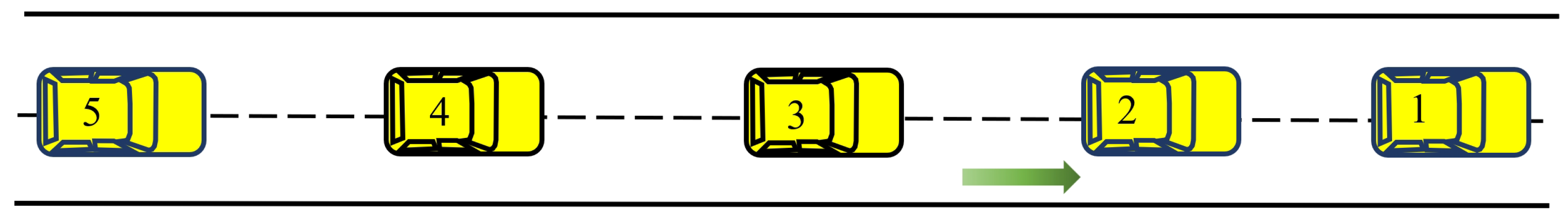
To assess the limitations associated with implementing a fixed maximum speed, this study simulates a five-vehicle platoon operating within a single-lane, straight-road traffic scenario. The platoon consists of a leading vehicle (designated as vehicle 1) followed by four trailing vehicles (designated as vehicles 2, 3, 4, and 5), as illustrated in Figure 1. The sensitivity coefficients of $\kappa$ and $\lambda$ are 0.41 and 0.2, respectively. The road speed limit and the maximum speed are both set to 18 m/s.

3.1. Appropriate Maximum Speed Setting

The leading vehicle’s speed varies based on road speed limits, traffic conditions, and driver behavior, which significantly influences the speed and stability of the entire platoon. It follows a three-phase strategy: acceleration at 2 m/s² until it reaches the road speed limit, maintaining a constant speed for 30 s, and deceleration at −2 m/s² until traffic flow stabilizes. The speed of the preceding vehicle is defined as follows:

$$v_1\left(t\right)=\left\{\begin{array}{cc}{a}_{\mathrm{acc}}·t,\hfill & \mathrm{if}0\le t\le t_{\mathrm{acc}}\hfill \\ v_{\max },\hfill & \mathrm{if}{t}_{\mathrm{acc}}<t\le t_{\mathrm{acc}}+t_{\mathrm{const}}\hfill \\ v_{\max }+a_{\mathrm{dec}}·\left(t-t_{\mathrm{acc}}-t_{\mathrm{const}}\right),\hfill & \mathrm{if}{t}_{\mathrm{acc}}+t_{\mathrm{const}}<t\le t_{\mathrm{acc}}+t_{\mathrm{const}}+t_{\mathrm{dec}}\hfill \\ 0,\hfill & \mathrm{if}t>t_{\mathrm{acc}}+t_{\mathrm{const}}+t_{\mathrm{dec}}\hfill \end{array}\right.$$

(4)

where $v_1\left(t\right)$ denotes the speed of the leading vehicle of the platoon at time t. The acceleration $a_{\mathrm{acc}}=2{\mathrm{m}/\mathrm{s}}^2$ represents the acceleration of the first vehicle; the deceleration $a_{\mathrm{dec}}=-2{\mathrm{m}/\mathrm{s}}^2$ represents the deceleration of the first vehicle; the speed $v_{\max }=18\mathrm{m}/\mathrm{s}$ is the speed of the leading vehicle during the constant-speed phase. The acceleration time $t_{\mathrm{acc}}=9\mathrm{s}$, calculated as $t_{\mathrm{acc}}={\displaystyle \frac{v_{\max }}{a_{\mathrm{acc}}}}$; the constant-speed duration $t_{\mathrm{const}}=30\mathrm{s}$; and the deceleration time $t_{\mathrm{dec}}=9\mathrm{s}$, calculated as $t_{\mathrm{dec}}={\displaystyle \frac{v_{\max }}{\left|a_{\mathrm{dec}}\right|}}$.

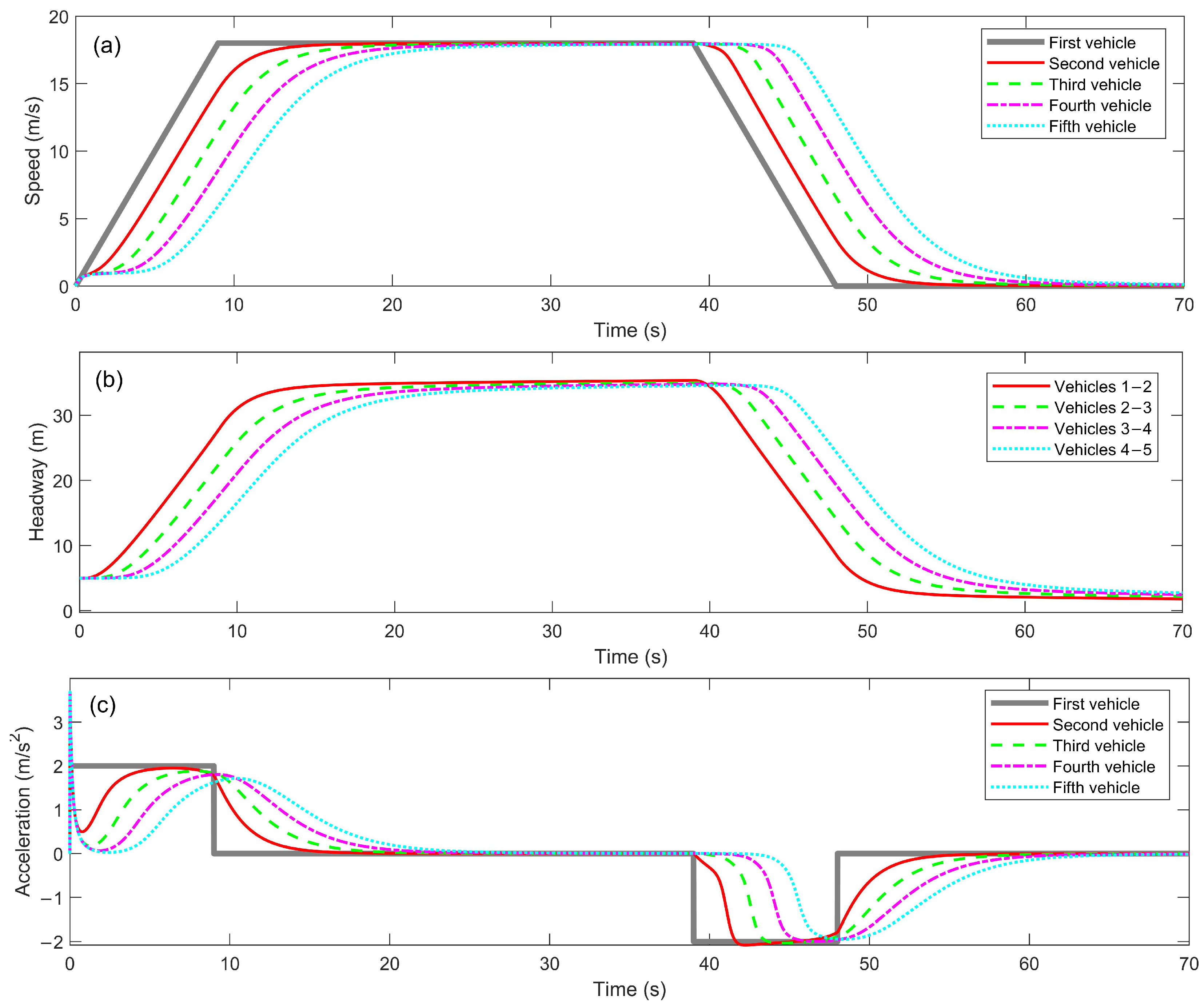
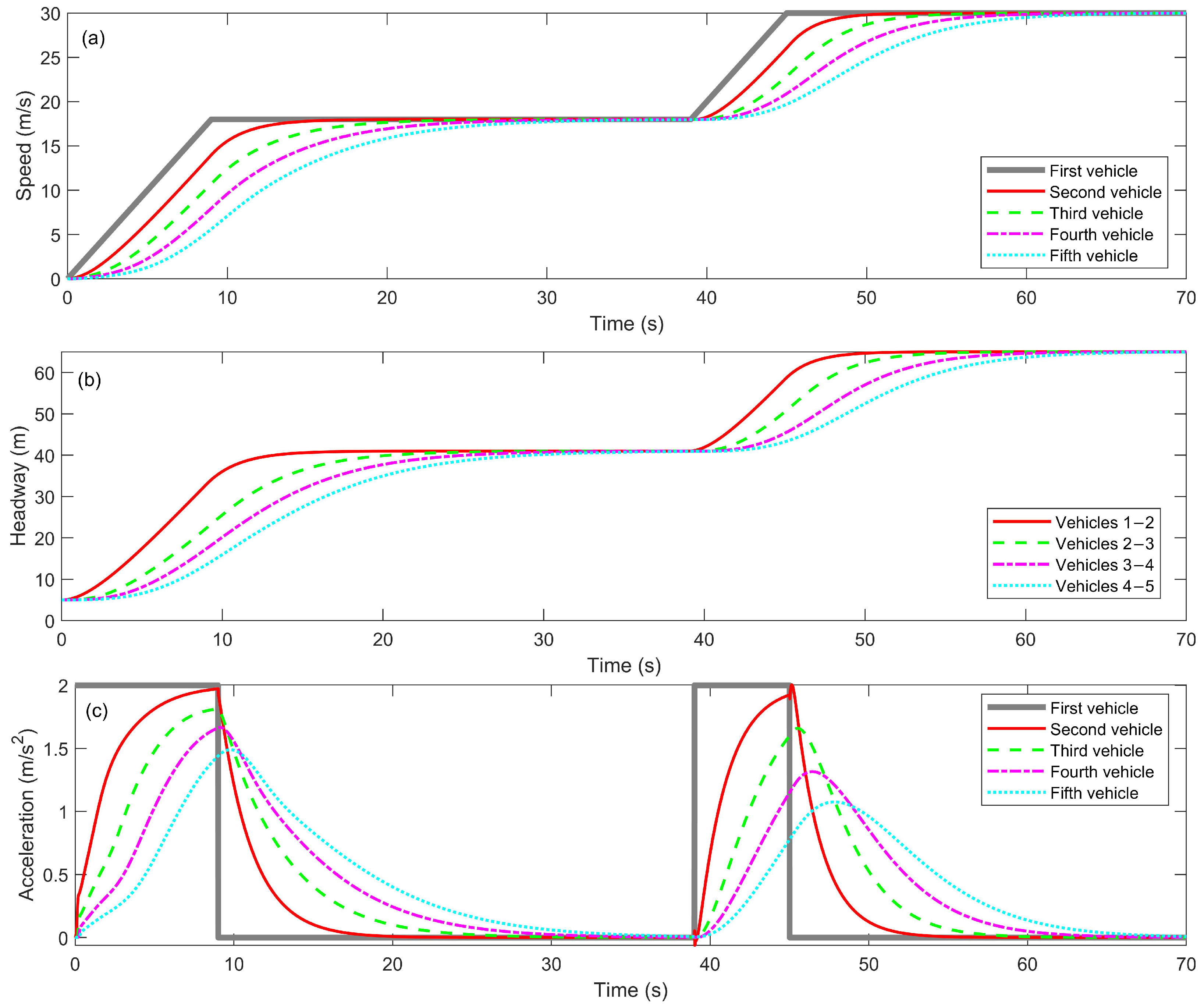
When the maximum speed of the platoon’s leading vehicle is used to determine the maximum speed in the OVF for the following vehicles, the evolution of the platoon traffic flow is shown in Figure 2. Figure 2a displays the speed of the five vehicles within the platoon, Figure 2b shows the headway between adjacent vehicles, and Figure 2c presents the acceleration of the five vehicles.

From the perspective of platoon evolution, the CFM demonstrates some key performance characteristics in the dynamic changes of speed, headway, and acceleration. In Figure 2a, the speed evolution of the five vehicles within the platoon is clearly visible. The leading vehicle quickly reaches its maximum speed of 18 m/s and maintains a constant speed, then begins decelerating around 40 s until it comes to a complete stop. The following vehicles exhibit noticeable lag in both the acceleration and deceleration phases: their speed increases and decreases more slowly than that of the leading vehicle, reflecting the propagation characteristics of “elastic waves” within the platoon. Although the following vehicles gradually approach the speed of the leading vehicle during the constant speed phase, there is still some speed deviation, indicating a delay in the model’s dynamic response.

The evolution of headway is shown in Figure 2b. It increases during the acceleration phase, indicating that the following vehicles need to maintain a greater distance within the platoon to ensure safety while catching up to the leading vehicle. During the constant speed phase, the headway between vehicles stabilizes, demonstrating that the CFM maintains a reasonable inter-vehicle distance within the platoon, contributing to overall platoon stability. In the deceleration phase, the headway decreases proportionally as vehicles reduce their speed in response to the leading vehicle’s deceleration, maintaining safety.

The dynamic changes in acceleration are illustrated in Figure 2c. The acceleration curve of the leading vehicle exhibits a typical acceleration-constant speed-deceleration pattern, while the following vehicles show a “buffering” effect, characterized by reduced peak acceleration and extended duration. This transitional characteristic reflects the propagation of “gradual waves” within the platoon, as following vehicles gradually stabilize their acceleration responses.

Thanks to the appropriate setting of the maximum speed, the CFM accurately simulates the dynamic characteristics of vehicles within the platoon during acceleration, constant speed, and deceleration phases. During acceleration, the model effectively captures the gradual increase in vehicle speeds, ensuring safe and expanded inter-vehicle distances. In the constant speed phase, following vehicles effectively track the leading vehicle’s speed, demonstrating good platoon stability. During deceleration, following vehicles respond promptly to the leading vehicle’s deceleration, maintaining safe headways. Overall, the CFM demonstrates high accuracy and stability across all driving phases, effectively preventing speed fluctuations and abrupt headway changes that could compromise platoon stability.

3.2. Inappropriate Maximum Speed Setting

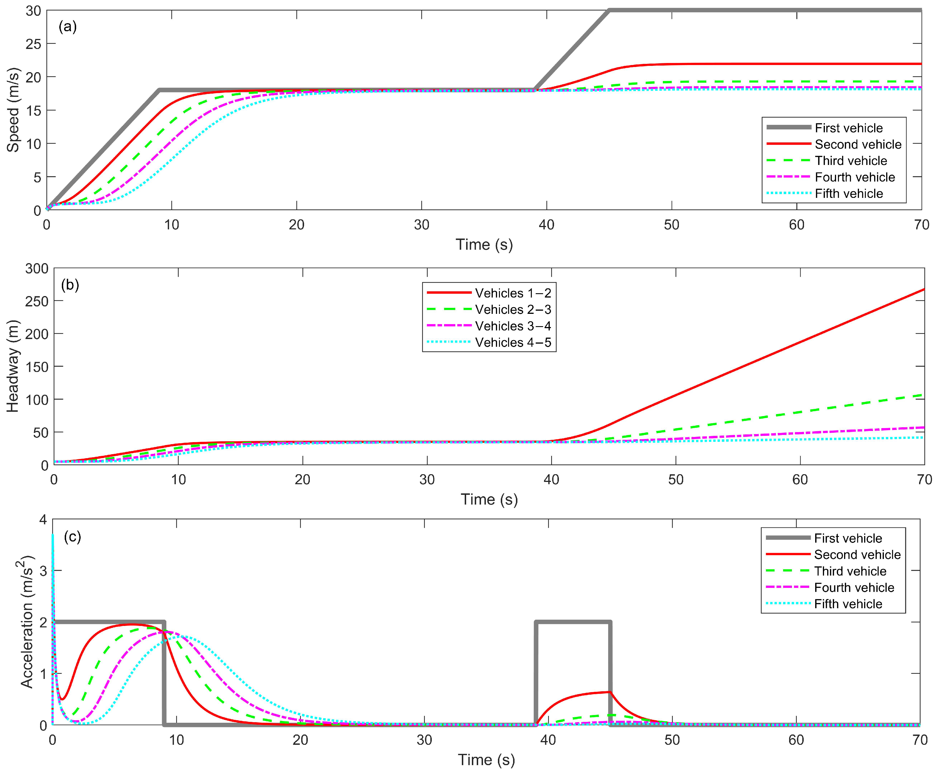
When the first vehicle acts as the platoon leader, its driving state is defined by specific speed and acceleration settings, while the following four vehicles within the platoon are simulated based on the CFM. The leading vehicle accelerates from 0 m/s to 18 m/s at an acceleration of 2 m/s², maintaining a constant speed for 30 s. It then accelerates again from 18 m/s to 30 m/s at the same rate and continues at 30 m/s until the end of the total simulation time (70 s). Throughout this process, the maximum speed of the following four vehicles in the platoon is set to 18 m/s. This simulation scenario represents the transition of the platoon leader from a low-speed segment to a high-speed segment.

The purpose of this simulation is to demonstrate the limitations of using a fixed maximum speed within the platoon in the CFM, highlighting the inability of following vehicles to maintain pace when the platoon leader travels at a higher speed, potentially resulting in platoon instability.

The speed of the platoon leader can be expressed by the following piecewise function:

$$v_1\left(t\right)=\left\{\begin{array}{cc}{a}_{\mathrm{acc}}·t,\hfill & \mathrm{if}0\le t\le t_{\mathrm{acc}1}\hfill \\ v_{\mathrm{phase}1},\hfill & \mathrm{if}{t}_{\mathrm{acc}1}<t\le t_{\mathrm{acc}1}+t_{\mathrm{const}1}\hfill \\ v_{\mathrm{phase}1}+a_{\mathrm{acc}}·\left(t-t_{\mathrm{acc}1}-t_{\mathrm{const}1}\right),\hfill & \mathrm{if}{t}_{\mathrm{acc}1}+t_{\mathrm{const}1}<t\le t_{\mathrm{acc}1}+t_{\mathrm{const}1}+t_{\mathrm{acc}2}\hfill \\ v_{\max },\hfill & \mathrm{if}{t}_{\mathrm{acc}1}+t_{\mathrm{const}1}+t_{\mathrm{acc}2}<t\le 70\mathrm{s}\hfill \end{array}\right.$$

(5)

where $a_{\mathrm{acc}}$ represents the acceleration phase’s acceleration, set to $2{\mathrm{m}/\mathrm{s}}^2$; $v_{\mathrm{phase}1}$ represents the speed in the first constant speed phase, set to $18\mathrm{m}/\mathrm{s}$; $v_{\max 1}$ represents the speed in the second constant speed phase, set to $30\mathrm{m}/\mathrm{s}$; $t_{\mathrm{acc}1}$ is the acceleration time for the first phase, calculated as:

$$t_{\mathrm{acc}1}={\displaystyle \frac{v_{\mathrm{phase}1}}{a_{\mathrm{acc}}}}={\displaystyle \frac{18\mathrm{m}/\mathrm{s}}{2{\mathrm{m}/\mathrm{s}}^2}}=9\mathrm{s};$$

(6)

$t_{\mathrm{const}1}$ is the duration of the first constant speed phase, set to $30\mathrm{s}$; $t_{\mathrm{acc}2}$ is the acceleration time for the second phase, calculated as:

$$t_{\mathrm{acc}2}={\displaystyle \frac{v_{\max 1}-v_{\mathrm{phase}1}}{a_{\mathrm{acc}}}}={\displaystyle \frac{30\mathrm{m}/\mathrm{s}-18\mathrm{m}/\mathrm{s}}{2{\mathrm{m}/\mathrm{s}}^2}}=6\mathrm{s}.$$

(7)

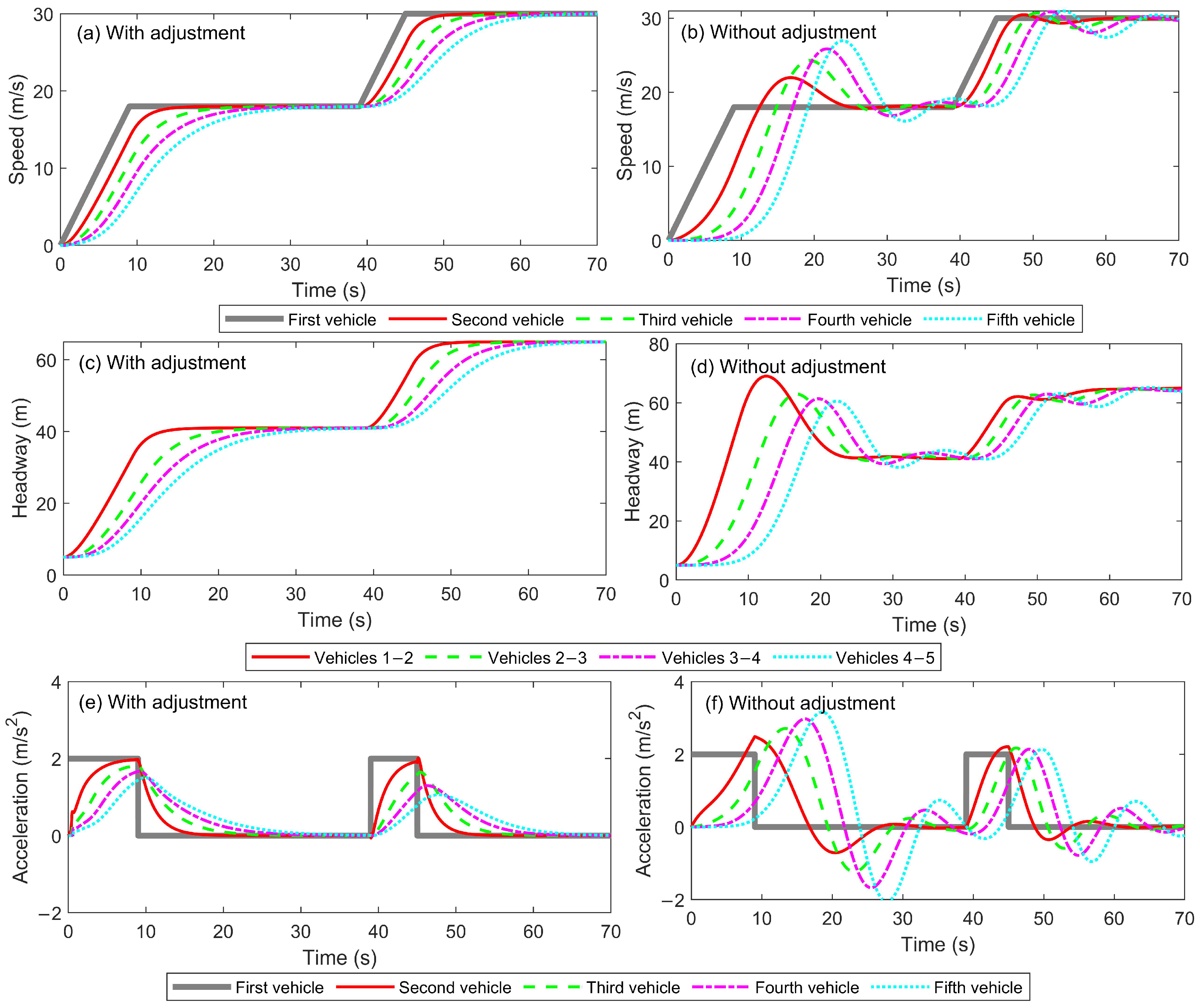
Figure 3 illustrates the evolution of the platoon traffic flow when the following vehicles are subject to a fixed maximum speed while the platoon leader exceeds this limit. Figure 3a depicts the speeds of the five vehicles within the platoon. As the platoon leader accelerates from 18 m/s to 30 m/s, the following four vehicles, constrained by their fixed maximum speed of 18 m/s, cannot accelerate further and can only maintain this speed. This constraint prevents the following vehicles within the platoon from fully responding to the acceleration of the leader, resulting in their speeds remaining constant between 40 s and 70 s. Consequently, they are unable to increase their speeds to match that of the platoon leader. During the second constant-speed phase, the speed deviations of the following vehicles relative to the platoon leader were 26.9%, 35.7%, 38.6%, and 38.7%, respectively. This significant speed difference clearly highlights the limitations of a fixed maximum speed: as the leader continues to accelerate, the following vehicles within the platoon fail to keep pace, negatively impacting platoon continuity and stability.

Figure 3b shows the headway evolution within the platoon. During the acceleration phases, the headway gradually increases, especially when the leader accelerates from 18 m/s to 30 m/s, causing a sharp increase in inter-vehicle distances. The most noticeable headway increase occurs between the first and second vehicles (red curve), which shows a rapid upward trend after 40 s. This is because the second vehicle, restricted to a speed of 18 m/s, cannot continue accelerating to catch up with the leader, causing the gap to widen rapidly. This abrupt change in headway indicates that a fixed maximum speed constraint negatively affects platoon stability, potentially causing platoon breakup, reduced traffic efficiency, and significant safety risks in real driving scenarios.

Figure 3c illustrates acceleration dynamics within the platoon. During the initial acceleration and constant-speed phases of the platoon leader, the following vehicles gradually adjust their accelerations, exhibiting a tendency towards stability. However, when the leader further accelerates from 18 m/s to 30 m/s, the acceleration of following vehicles essentially drops to zero, as they have already reached their fixed maximum speed of 18 m/s and cannot accelerate further.

The primary limitation of employing a fixed maximum speed within the platoon becomes evident when the platoon leader accelerates beyond this set limit: following vehicles are unable to match the leader’s speed in a timely manner. This results in pronounced speed desynchronization and rapidly increasing headway distances, especially between the leader and the first follower, as the followers cannot continue to accelerate to keep pace with the leader. The resulting mismatch not only leads to delayed dynamic acceleration responses but may also cause the platoon to become elongated or even fragmented, ultimately reducing platoon continuity and overall traffic flow efficiency. Persistent speed and headway errors increase the risk of losing platoon integrity and elevate safety risks. These findings highlight the critical importance of dynamically and appropriately setting the maximum speed parameter in car-following models. Only by estimating and adjusting maximum vehicle speeds in real time can the platoon effectively adapt to varying traffic conditions, maintain stable and cohesive formation, and ensure accurate, safe, and efficient driving behavior in diverse, real-world environments.

4. Adaptive CFM with UKF-Based Maximum Speed Estimation

To estimate the maximum speed parameter in the optimal velocity function of a CFM for platoon control, this study proposes utilizing the UKF. The UKF is a highly effective nonlinear filtering technique specifically designed to address the nonlinear dynamics commonly encountered in CFMs. Unlike the extended Kalman filter (EKF), which approximates the system by linearizing it around an operating point, the UKF employs an unscented transformation to propagate a carefully selected set of sigma points directly through the nonlinear dynamic model of vehicle platoons. This method avoids linearization altogether, enabling the UKF to more accurately capture the complex, nonlinear behaviors typical in platoon dynamics. As a result, the UKF provides more precise parameter estimates and demonstrates superior performance under dynamic platoon conditions, where linear approximations are often inadequate.

The proposed CFM is constructed based on several designed rules and assumptions. First, it is assumed that each following vehicle can obtain real-time information about the speed and acceleration of the preceding vehicle, either via V2V communication or through onboard sensors. All vehicles are modeled as operating in a single-lane, longitudinal following scenario, without considering lane-changing, merging, or platoon splitting. Each vehicle is assumed to follow the OVF, wherein the maximum speed parameter is dynamically estimated via the UKF according to the state information of the immediately preceding vehicle. Additionally, the model presumes that all vehicles within the platoon participate cooperatively in speed synchronization and headway control.

The vehicle dynamics within the platoon, described by a nonlinear CFM incorporating the optimal velocity function, treat the maximum speed as an unknown parameter requiring estimation. The UKF algorithm iteratively updates this parameter by integrating real-time observational data such as vehicle speeds and headways within the platoon. Initial assumptions about system state and measurement noise distributions are established, from which sigma points are generated to predict state propagation through the nonlinear model. These predictions are then continuously updated based on real-time measurements, yielding an optimal, dynamically adaptive estimate of the maximum speed parameter.

The specific application scenarios for the proposed model include coordinated speed control and platoon management in connected and autonomous vehicle (CAV) systems, especially on highways, expressways, or dedicated lanes where variable speed limits, frequent acceleration/deceleration, or changes in the platoon leader may occur. The model is also well-suited for intelligent transportation systems that leverage real-time communication and sensor data to achieve dynamic platoon coordination, such as in smart city environments or during autonomous vehicle convoys.

4.1. Vehicle State Transition Equation

By utilizing V2V communication, information such as the speed, acceleration, and other state variables of the preceding vehicle can be obtained and used for control of platoon vehicles. The vehicle state transition equation is used to predict the motion states of the vehicle during the car-following process.

In this study, the maximum speed $v_{\max ,k}$, the velocity of the target vehicle $v_{t,k}$, and the headway $d_k$ between the target and ego vehicles are selected as the state vector to comprehensively describe vehicle dynamics. This choice is based on the following considerations: the maximum speed parameter directly determines the vehicle’s optimal speed and influences the overall speed coordination of the platoon, making it a key variable for improving the CFM; the velocity of the target vehicle serves as an essential reference for the following vehicle’s decisions and is crucial for the platoon’s timely response; and the headway directly affects both driving safety and ride comfort. By estimating these three critical state variables in real time, the improved UKF algorithm can significantly enhance the platoon’s car-following performance and stability under dynamic conditions. The vehicle state transition equation is given by:

$${\mathbf{x}}_k=f({\mathbf{x}}_{k-1},{\mathbf{u}}_{k-1})+{\mathbf{w}}_{k-1},$$

(8)

where ${\mathbf{x}}_k$ is the state vector at the time k, and ${\mathbf{x}}_k=[v_{\max ,k};v_{t,k};d_k]$ . $f(·)$ is the state transition function that describes the transition from time $k-1$ to time k, ${\mathbf{u}}_{k-1}$ is the control input, and ${\mathbf{w}}_{k-1}$ is the process noise, which is usually assumed to be zero-mean Gaussian noise with covariance $\mathbf{Q}$.

When the vehicle is in a car-following state, the state transition function is:

$$f\left({\mathbf{x}}_{k-1}\right)=\left[\begin{array}{c}{v}_{\max ,k-1}\\ v_{t,k-1}+a_{t,k-1}T\\ d_{k-1}+x_{e,k-1}-x_{t,k-1}\end{array}\right]$$

(9)

where T is sample time. $a_{t,k-1}$, $v_{t,k-1}$, and $x_{t,k-1}$ are the acceleration, velocity, and the displacement of the target vehicle at time $k-1$, respectively. $x_{e,k-1}$ is the displacement of the ego vehicle at time $k-1$. They are defined as follows:

$$a_{t,k-1}=\kappa \left[{\displaystyle \frac{v_{\max ,k-1}}{2}}tanh(d_{k-1}-h_c)+tanh\left(h_c\right)-v_{t,k-1}\right]+\lambda \Delta v_{k-1},$$

(10)

$$x_{t,k-1}=v_{t,k-1}T+0.5a_{t,k-1}{T}^2,$$

(11)

$$x_{e,k-1}=v_{e,k-1}T+0.5a_{e,k-1}{T}^2,$$

(12)

where $a_{e,k-1}$ is the acceleration the ego vehicle at time $k-1$, and $\Delta v_{k-1}$ is the relative velocity between the target vehicle and the ego vehicle, which is expressed as following:

$$\Delta v_{k-1}=v_{e,k-1}-v_{t,k-1}.$$

(13)

The update of $v_{\max }$ via the UKF enables each following vehicle to dynamically adapt to the speed fluctuations of the preceding vehicle under varying road speed limits. This adaptive mechanism enhances overall speed synchronization within the platoon and contributes to improved platoon stability.

4.2. Measurement Equation

The speed of the ego vehicle and the corresponding safety headway are used as the measurements because both variables directly correspond to key components of the state vector—vehicle speed and headway—and can be reliably obtained using modern vehicle sensors. The UKF is employed to estimate the maximum speed of the OFV for the following vehicle, so that the calculated driving state of the following vehicle approaches that of the ego vehicle, and the headway reaches the safety headway defined by Equation (3). The measurement equation is defined as:

$${\mathbf{z}}_k=h\left({\mathbf{x}}_k\right)+{\mathbf{v}}_k,$$

(14)

where ${\mathbf{z}}_k$ is the measurement vector at time k, and ${\mathbf{z}}_k=[v_{e,k};d_{e,k}]$. $d_{e,k}$ and $v_{e,k}$ are the safe distance and the speed of the ego vehicle at time k. $h(·)$ is the measurement function that describes the relationship between the state vector and the measurement values, and ${\mathbf{v}}_k$ is the measurement noise, which is also typically assumed to be zero-mean Gaussian noise with covariance $\mathbf{R}$.

The measurement equation is used to calculate the predicted value of the measurement variable, and therefore should be expressed as a function of the state variable. The relationship between the target vehicle’s speed and the ego vehicle’s speed in the measurement function satisfies the following equation:

$$v_{e,k}=h_1\left(x_k\right)=v_{t,k}.$$

(15)

The safe distance corresponding to the current speed of the ego vehicle satisfies the following equation:

$$d_{e,k}=h_2\left(x_k\right)=d_k.$$

(16)

Finally, the measurement equation is expressed as:

$$h\left(x_k\right)=[h_1\left(x_k\right);h_2\left(x_k\right)].$$

(17)

The UKF corrects the state variables—maximum speed, vehicle speed, and headway—by comparing the predicted values of ego vehicle speed and safety headway (derived from the state estimate) with actual sensor measurements. The difference between predicted and measured values is used to update the state estimate, ensuring that the model remains closely aligned with real driving conditions.

4.3. Algorithm of Adaptive UKF

The Unscented Kalman Filter (UKF) is a nonlinear filtering method that does not require the assumption of linear relationships between state variables or between observations and state variables. However, in practical applications, sensor measurements are frequently affected by various sources of noise and interference, resulting in significant uncertainty in the measurement noise characteristics [37]. When the measurement noise variance is unknown or varies over time, the estimation accuracy of the conventional UKF can decrease markedly, and the algorithm may even diverge. To address the challenges posed by uncertain and time-varying measurement noise arising from sensor disturbances, this study employs an adaptive UKF, which can automatically adjust its noise covariance estimates. This adaptive capability enhances the robustness of the filter and ensures reliable state estimation. The algorithm of the adaptive UKF is as follows:

Building on the vehicle state transition equation and measurement equation introduced above, the nonlinear discrete state-space model of the vehicle-following system is established as follows:

$$\left\{\begin{array}{c}{\mathbf{x}}_k=f({\mathbf{x}}_{k-1},{\mathbf{u}}_{k-1})+{\mathbf{w}}_{k-1}\hfill \\ {\mathbf{z}}_k=h\left({\mathbf{x}}_k\right)+{\mathbf{v}}_k\hfill \end{array}\right..$$

(18)

Generate the set of sigma points based on the current state estimate for state propagation, thereby enabling an accurate approximation of the state mean and covariance under nonlinear dynamics:

$${\mathbf{X}}_k^{\left(i\right)}={\widehat{\mathbf{x}}}_k+\left\{\begin{array}{cc}0,\hfill & \mathrm{if}i=0\hfill \\ \sqrt{(n+\lambda ){\mathbf{P}}_k(:,i)},\hfill & \mathrm{if}1\le i\le n\hfill \\ -\sqrt{(n+\lambda ){\mathbf{P}}_k(:,i-n)},\hfill & \mathrm{if}n+1\le i\le 2n\hfill \end{array}\right.,$$

(19)

where ${\widehat{\mathbf{x}}}_k$ is the current state estimate, ${\mathbf{P}}_k$ is the state covariance matrix, and n is the dimension of the state vector. $\lambda$ is the scaling parameter and defined as follows:

$$\lambda ={\rho }^2(n+\kappa )-n,$$

(20)

where $\rho$ is a positive constant, while $\kappa$ is a second scaling factor that is usually set to 0.

Calculate the one-step prediction for the $2n+1$ Sigma points:

$${\mathbf{X}}_{k+1|k}^{\left(i\right)}=f\left({\mathbf{X}}_k^{\left(i\right)}\right).$$

(21)

Calculate the one-step predicted state and its covariance matrix, using the predicted Sigma points and the corresponding weights. The predicted state and the error covariance of predicted state are given by:

$${\widehat{\mathbf{x}}}_{k+1|k}=\sum _{i=0}^{2L}{W}_m^{\left(i\right)}{\mathbf{X}}_{k+1|k}^{\left(i\right)},$$

(22)

$${\mathbf{P}}_{k+1|k}=\sum _{i=0}^{2L}{W}_c^{\left(i\right)}\left({\mathbf{X}}_{k+1|k}^{\left(i\right)}-{\widehat{\mathbf{x}}}_{k+1|k}\right){\left({\mathbf{X}}_{k+1|k}^{\left(i\right)}-{\widehat{\mathbf{x}}}_{k+1|k}\right)}^T+\mathbf{Q},$$

(23)

where $W_m^{\left(i\right)}$ and $W_c^{\left(i\right)}$ are the corresponding weights, and they are defined as:

$$W_m^i=\left\{\begin{array}{cc}{\displaystyle \frac{\lambda }{n+\lambda }},\hfill & \mathrm{if}i=0\hfill \\ {\displaystyle \frac{0.5\lambda }{n+\lambda }},\hfill & \mathrm{if}i=1,\dots ,2n\hfill \end{array}\right.,$$

(24)

$$W_m^i=\left\{\begin{array}{cc}{W}_c^{\left(0\right)}={\displaystyle \frac{\lambda }{n+\lambda }}+(1-{\alpha }^2+\beta ),\hfill & \mathrm{if}i=0\hfill \\ W_c^{\left(i\right)}={\displaystyle \frac{1}{2(n+\lambda )}},\hfill & \mathrm{if}i=1,\dots ,2n\hfill \end{array}\right.,$$

(25)

where $\alpha$ and $\beta$ are parameters of the UKF, used to control the distribution of sigma points. $\alpha$ is usually set to a small positive value (e.g., $\alpha =1\times {10}^{-3}$), while $\beta$ is used to incorporate prior knowledge of the distribution (e.g., $\beta =2$ for Gaussian distribution).

Use the predicted Sigma points from step 3 in the measurement equation to obtain the predicted measurement value:

$${\mathbf{Z}}_{k+1|k}^{\left(i\right)}=h\left({\mathbf{X}}_{k+1|k}^{\left(i\right)}\right).$$

(26)

Calculate the predicted measurement mean and covariance, as well as the cross covariance between the state and the measurements, based on the Sigma points in the measurement space using the following equations:

$${\widehat{\mathbf{z}}}_{k+1|k}=\sum _{i=0}^{2n}{W}_m^{\left(i\right)}{\mathbf{Z}}_{k+1|k}^{\left(i\right)},$$

(27)

$${\mathbf{P}}_{zz}=\sum _{i=0}^{2n}{W}_c^{\left(i\right)}\left({\mathbf{Z}}_{k+1|k}^{\left(i\right)}-{\widehat{\mathbf{z}}}_{k+1|k}\right){\left({\mathbf{Z}}_{k+1|k}^{\left(i\right)}-{\widehat{\mathbf{z}}}_{k+1|k}\right)}^T+\mathbf{R},$$

(28)

$${\mathbf{P}}_{xz}=\sum _{i=0}^{2n}{W}_c^{\left(i\right)}\left({\mathbf{X}}_{k+1|k}^{\left(i\right)}-{\widehat{\mathbf{x}}}_{k+1|k}\right){\left({\mathbf{Z}}_{k+1|k}^{\left(i\right)}-{\widehat{\mathbf{z}}}_{k+1|k}\right)}^T.$$

(29)

The measurement noise covariance matrix is adaptively adjusted based on recent innovation (or residual) statistics, enabling the filter to automatically tune itself in response to changes in measurement noise and thereby enhancing estimation robustness, as follows:

$${\mathbf{R}}_k=(1-j_k){\mathbf{R}}_{k-1}+j_k{\mathbf{V}}_k{\mathbf{V}}_k^T,$$

(30)

where $j_k$ is the forgetting factor, defined as $j_k=(1-b)/(1-b^k)$, with b as the forgetting factor, typically taken as $0.995$, and $V_k$ is represent the innovation and expressed as follows:

$${\mathbf{V}}_{k+1}={\mathbf{z}}_{k+1}-{\widehat{\mathbf{z}}}_{k+1|k}$$

(31)

where ${\mathbf{z}}_{k+1}$ is the actual measurement value, and ${\widehat{\mathbf{z}}}_{k+1|k}$ is the predicted measurement mean.

Calculate the Kalman gain, which balances the uncertainty between the state prediction and the measurement to achieve optimal state correction:

$$\mathbf{K}={\mathbf{P}}_{xz}{\mathbf{P}}_{zz}^{-1}.$$

(32)

Finally, update the system state and covariance matrix by incorporating the Kalman gain and the measurement innovation, so that the estimated state is corrected based on the new measurement and the overall uncertainty is reduced:

$${\widehat{\mathbf{x}}}_{k+1}={\widehat{\mathbf{x}}}_{k+1|k}+\mathbf{K}\left({\mathbf{z}}_{k+1}-{\widehat{\mathbf{z}}}_{k+1|k}\right),$$

(33)

$${\mathbf{P}}_{k+1}={\mathbf{P}}_{k+1|k}-\mathbf{K}{\mathbf{P}}_{zz}{\mathbf{K}}^T.$$

(34)

Figure 4 illustrates the overall process for estimating a vehicle’s maximum speed using an Unscented Kalman Filter (UKF). The main simulation cycle follows a logical sequence from “Start numerical simulation” to “Vehicle state update for following vehicles” on the left side of the diagram. On the right, the key steps of the UKF at each simulation step are depicted, including parameter initialization, Sigma point generation, state prediction and measurement prediction via an unscented transformation, Kalman gain computation, and the subsequent state and covariance updates.

In each iteration, real-time data such as speed, acceleration, and headway from the preceding vehicle are obtained via V2V communication (or onboard sensors) and incorporated into the measurement update step of the UKF. These measurements feed into the vehicle state transition and measurement equations, enabling the filter to continuously refine estimates of the maximum speed. This integration ensures the model remains responsive to rapid changes in the leading vehicle’s behavior, thereby improving the adaptive response of the following vehicles and enhancing overall traffic flow stability.

5. Performance Evaluation of Platoon Speed Control

By using UKF, the maximum speed parameter in the CFM can be adaptively adjusted, enabling the traditional CFM to accommodate a wider range of real-world driving scenarios. For instance, this improved CFM is suitable for continuous driving on roads with varying speed limits or for maintaining consistent following distance when the platoon leader changes speed. The performance of the adaptive CFM is compared with that of the traditional CFM under various traffic conditions such as start, stop, acceleration, and deceleration to highlight the advantages of the adaptive approach.

5.1. Single Acceleration Scenario

Before the simulation begins, the initial speed of each vehicle is 0 m/s, and the headway is the minimum safe distance of 5 m. After the simulation starts, the leading vehicle of the traffic flow begins to accelerate to desired speed of 30 m/s over a period of 15 s. Once the desired speed is reached, the leading vehicle continues to travel at a constant speed. In the traditional CFM, the maximum speeds of the following vehicles are fixed at 18 m/s. In the adaptive CFM, however, the maximum speeds of the following vehicles are dynamically estimated using an UKF, rather than being set to a fixed value. Figure 4 illustrates the evolution of speed, headway, and acceleration for all vehicles using the adaptive CFM proposed in this study, in comparison with the traditional CFM.

In the traditional CFM model (Figure 5a), the speeds of the four following vehicles fail to reach the final maximum speed of the leading vehicle, which accelerates to 10 m/s. Additionally, during the acceleration phase, there is a noticeable delay in the speed response of the following vehicles, preventing them from closely tracking the preceding vehicle’s acceleration changes. The primary reason for these phenomena is the mismatch between the maximum speed of the following vehicles and that of the leading vehicle, making it difficult for them to remain synchronized at the same speed level. This results from the mismatch between the fixed maximum speeds of the followers and the leader’s speed, causing desynchronized speeds and increased platoon instability.

In contrast, in the adaptive CFM model (Figure 5b), each vehicle is able to more synchronously and smoothly reach the leading vehicle’s final maximum speed. This is because the adaptive CFM dynamically adjusts the maximum speed of each vehicle based on real-time estimation of the preceding vehicle’s state, allowing the following vehicles to promptly respond to speed changes of the leading vehicle. The adaptive CFM achieves faster and more coordinated speed responses, markedly reducing delays and discrepancies compared to the traditional model. This leads to more stable headways, smoother acceleration, and enhanced overall traffic flow efficiency and safety. Additionally, the reduction in unnecessary acceleration and deceleration events can improve both driving comfort and energy economy, highlighting the adaptive model’s comprehensive advantages.

As shown in Figure 5c,d, there are significant differences in headway evolution between the traditional CFM and the adaptive CFM models. In the traditional CFM model (Figure 5c), as the leading vehicle continues to accelerate to 10 m/s, the second following vehicle is constrained by its maximum speed and cannot reach 10 m/s. As a result, the headway between the first and second vehicles continually increases once the leading vehicle’s speed exceeds 7 m/s. Additionally, as the influence of the leading vehicle on the subsequent following vehicles gradually weakens, a decreasing speed trend emerges: the second vehicle’s speed is higher than the third vehicle’s, the third vehicle’s speed is higher than the fourth vehicle’s, and so on. Due to the unsynchronized speeds of the vehicles, the headway fails to converge to a fixed value, reflecting the inability of the traditional CFM model to achieve stable following behavior in this scenario.

The adaptive CFM model dynamically estimates the maximum speed of each vehicle to adapt to the changes in the leading vehicle’s state. As a result, once the traffic flow stabilizes, the headway between all vehicles converges to a fixed value (Figure 5d), demonstrating the adaptive CFM’s advantage in handling the stability of multi-vehicle platoons. This model enables more effective and timely responses to speed changes, resulting in greater stability in following behavior. As a result, vehicle interactions become smoother, headway variations are minimized, and both the coordination and safety of the entire platoon are significantly improved.

In the traditional CFM (Figure 5e), the fixed maximum speed constraint of each following vehicle, coupled with its inability to dynamically adapt to the driving state of the leading vehicle, results in a pronounced acceleration spike when the leading vehicle initiates acceleration. After perceiving the acceleration of the preceding vehicle, each following vehicle, due to information transmission delay and speed differences, often needs to rapidly increase its acceleration to close the gap with the preceding vehicle, resulting in sharp fluctuations in acceleration. This sudden change not only leads to desynchronized acceleration responses among the following vehicles but also causes unstable oscillations in the traffic flow, reducing overall traffic efficiency.

In contrast, in the adaptive CFM (Figure 5f), the UKF algorithm dynamically estimates the maximum speed based on the driving state of the preceding vehicle. This enables the following vehicles to respond more smoothly to the preceding vehicle’s acceleration changes. When the preceding vehicle accelerates, the following vehicles do not need to make abrupt adjustments in acceleration. Instead, they gradually adapt to the preceding vehicle’s speed variations, using the smooth state estimates provided by the UKF. This results in a more controlled acceleration response, mitigating the sharp fluctuations in acceleration typically observed in traditional CFM. As a result, the acceleration curves for all following vehicles become more synchronized, exhibiting consistent acceleration and deceleration patterns. Consequently, the adaptive CFM achieves more stable and coordinated acceleration responses, greatly reducing spikes and sudden changes. This leads to enhanced traffic flow stability, improved ride comfort, and greater overall platoon safety and efficiency.

Figure 6 shows the vehicle displacement for the two CFMs. In the traditional CFM model (Figure 6a), the displacement curves of the following vehicles gradually lag behind that of the leading vehicle, especially during the acceleration phase. The response of each following vehicle is noticeably delayed, causing the displacement difference to continuously increase. Due to the maximum speed limit, the following vehicles struggle to close the gap with the leading vehicle quickly, resulting in reduced traffic flow efficiency. In the adaptive CFM model, the UKF dynamically estimates the state of the leading vehicle and adjusts the maximum speed of the following vehicles, allowing the displacement curves of the vehicles to more closely match that of the leading vehicle, significantly reducing the displacement difference (Figure 6b). During the acceleration phase, the displacement curves in the adaptive CFM are more synchronized, and the headway between vehicles tends to stabilize, effectively suppressing the “car-following oscillations” observed in the traditional CFM. This improvement enables the adaptive CFM to achieve tighter and more stable platoon following, enhancing the overall stability of the traffic flow and road capacity, particularly in scenarios involving frequent acceleration, where it shows higher adaptability and response speed.

Figure 7 illustrates the maximum speeds of the following vehicles in the adaptive CFM, estimated using the UKF algorithm based on the preceding vehicle’s driving state. The speed of the leading vehicle is its actual driving speed, while the maximum speed of each following vehicle is dynamically estimated through the UKF.

The estimated maximum speeds of the following vehicles show small oscillations before stabilizing, which is the UKF’s response to changes in the preceding vehicle’s state during dynamic adjustment. These fluctuations gradually diminish over time, and eventually, the estimated maximum speeds of all vehicles align closely with the speed of the leading vehicle. This adaptive CFM mechanism, by dynamically adjusting the speed limits of each vehicle, results in a smoother speed distribution across the platoon. It not only reduces the speed differences seen in traditional CFMs but also enhances the synchronization of the response, reduces fluctuations during acceleration, and significantly improves the overall stability and efficiency of traffic flow.

5.2. Intermittent Acceleration Scenario

The motion of the leading vehicle under the intermittent acceleration scenario is defined by Equation (5). Figure 3 shows the platoon state evolution under the traditional CFM, while Figure 8 illustrates the platoon state evolution under the adaptive CFM. Figure 8a illustrates the speed variation of each vehicle in the platoon under the adaptive CFM model. The leading vehicle starts from rest and gradually accelerates, ultimately reaching the target speed of 30 m/s. The following vehicles in the platoon, guided by the maximum speed dynamically estimated through the UKF, also progressively approach the speed of the leading vehicle, demonstrating good speed-following behavior. Since the adaptive CFM can dynamically adjust the maximum speed of each vehicle based on the state of the leading vehicle, each following vehicle is able to respond quickly during the acceleration phase and gradually synchronize its speed with the leading vehicle, thus, achieving high-speed synchronization. This dynamic adjustment significantly reduces speed differences, suppresses traffic flow fluctuations caused by speed inconsistencies, and enhances the overall stability of the platoon traffic flow.

Figure 8b illustrates the variation in headways between platoon vehicles. Under the influence of the adaptive CFM, as the speed increases, the headways between platoon vehicles gradually increase and eventually stabilize. During the acceleration phase, the headway expands rapidly, indicating that the following vehicles are able to appropriately increase the gap with the leading vehicle, thereby avoiding collision risks associated with acceleration. Once the leading vehicle stops accelerating, the headways of the following vehicles also quickly stabilize. This stable adjustment of headways demonstrates the adaptive CFM’s effective control over platoon spacing, contributing to the formation of a uniform platoon flow, reducing traffic fluctuations caused by unstable headways, and highlighting the advantages of the adaptive CFM in smoothing platoon traffic flow control.

Figure 8c illustrates the acceleration variation of each platoon vehicle during the acceleration phases. With the support of the UKF, the adaptive CFM can smoothly control the acceleration of each vehicle, allowing the following vehicles to gradually respond to changes in the speed of the preceding vehicle, thus, avoiding sharp fluctuations in acceleration. By predicting the state of the preceding vehicle through the UKF, the adaptive CFM suppresses the abrupt acceleration changes commonly seen in traditional CFMs, ensuring a smoother acceleration response from the following vehicles, which follows a consistent trend. This smooth acceleration control reduces passenger discomfort and mitigates the platoon traffic flow instability caused by sudden acceleration changes, further improving the overall traffic flow efficiency and safety.

By comparing the speed, headway, and acceleration changes in Figure 3 and Figure 8, the adaptive CFM demonstrates significant advantages in dynamic responsiveness, stability, and platoon traffic efficiency. In the traditional CFM, speed responses exhibit noticeable delays, with increasing speed differences among vehicles during the acceleration phase, leading to unsynchronized platoon movement. In contrast, the adaptive CFM dynamically adjusts the maximum speed through the UKF, enabling platoon vehicles to quickly and smoothly respond to the leading vehicle’s speed changes, ultimately achieving speed synchronization.

Figure 9 illustrates the maximum speed estimation of each following vehicle in the platoon through the UKF algorithm, with the speed of the leading vehicle representing the actual driving speed. The maximum speeds of the subsequent platoon members are gradually estimated based on the state of the leading vehicle. During the two acceleration phases, the leading vehicle’s maximum speed reaches approximately 18 m/s and 30 m/s, respectively. The estimated maximum speeds of the following vehicles rise rapidly during each acceleration phase but lag slightly behind the leading vehicle and exhibit varying degrees of fluctuation. This lag and fluctuation occur because each following vehicle needs to gradually adjust its maximum speed based on the preceding vehicle’s state to maintain stable following in the dynamically changing traffic environment. The speed estimation curve of the second vehicle closely follows that of the leading vehicle, responding quickly with minimal lag and fluctuation. In contrast, the speed estimations of subsequent vehicles (such as the third, fourth, and fifth vehicles) exhibit increasing lag and fluctuation, indicating that as the distance from the leading vehicle increases, the delay and instability in speed estimation accumulate. After the two acceleration phases, the maximum speed estimates of all vehicles gradually stabilize and approach the actual speed of the leading vehicle, highlighting the advantages of the UKF in dynamic speed estimation, which effectively reduces fluctuations and achieves speed synchronization. This dynamic estimation mechanism enables each vehicle in the platoon to effectively adjust its maximum speed, maintain coordination with the leading vehicle, and enhance the overall stability and efficiency of the traffic flow.

5.3. Robustness Analysis

Adaptive adjustment of the measurement noise covariance matrix is vital for improving the accuracy and robustness of state estimation in dynamic environments. Measurement noise varies due to changes in sensor quality and environmental factors. By adapting the covariance matrix, the model accounts for these variations, maintaining accurate estimates despite changing noise characteristics. This enhances the balance between measurement data and model predictions, leading to more reliable and stable vehicle-following behavior within the platoon, thereby improving overall traffic flow safety and efficiency. This subsection investigates the robustness of the adaptive strategy under conditions of noise uncertainty, wherein the motion of the leading vehicle is characterized by an intermittent acceleration scenario.

Figure 10 compares the vehicle acceleration when the initial measurement noise covariance matrix is increased to 10,000 times its original value, while Figure 11 compares the corresponding maximum speed estimation accuracy with and without the adjustment of the covariance matrix due to measurement noise.

In terms of speed (Figure 10a,b), the adaptive adjustment (left side) enables the following vehicles to synchronize more smoothly with the leading vehicle’s speed, exhibiting less lag and superior coordination during both acceleration and deceleration phases. In contrast, the non-adaptive scenario (right side) shows noticeable delays and significant discrepancies in speed synchronization, resulting in larger speed differences within the platoon. Without adaptive adjustment of the measurement noise covariance matrix, the root mean square (RMS) values of velocity errors between the following vehicles and the leading vehicle are 2.84 m/s, 4.78 m/s, 6.22 m/s, and 7.36 m/s, respectively. With adaptive tuning, these RMS velocity errors are reduced to 1.63 m/s, 2.92 m/s, 4.03 m/s, and 5.01 m/s. The implementation of the adaptive adjustment approach achieves substantial error mitigation, resulting in reductions of 42.6%, 38.9%, 35.2%, and 31.9% in speed following discrepancies for the corresponding cases.

Regarding headway (Figure 10c,d), the adaptive adjustment maintains more stable headway with fewer fluctuations during the acceleration and deceleration phases, ensuring safer and more consistent distances between vehicles. Without adaptive adjustment, the headway increases erratically, especially when the leading vehicle accelerates, leading to instability in traffic flow. For acceleration (Figure 10e,f), the adaptive adjustment results in more synchronized and smoother acceleration transitions across the platoon vehicles, reducing sudden spikes and enhancing stability. In contrast, the non-adaptive adjustment results in uncoordinated acceleration profiles, with noticeable spikes and delays, indicating inefficiencies in traffic flow management. Comparative analysis of adaptive versus non-adaptive adjustment reveals significant suppression of RMS acceleration tracking errors, with reductions of 39.3%, 43.0%, 43.1%, and 41.9% across the four following vehicles. Overall, the adaptive adjustment of the measurement noise covariance matrix significantly improves speed synchronization, headway stability, and acceleration smoothness, thereby enhancing the overall traffic flow and vehicle-following stability.

In Figure 11a, the adaptive adjustment results in smoother and more accurate estimations, closely tracking the actual speed of the leading vehicle with minimal fluctuations. In contrast, Figure 11b shows greater deviations and slower convergence without the adaptive adjustment, highlighting the challenges in accurately estimating the maximum speed under dynamic conditions. Overall, the adaptive method enhances estimation accuracy, ensuring more reliable vehicle-following behavior and improved traffic flow stability, especially in complex, changing environments.

By comparing the evolution of vehicle states and the accuracy of maximum speed estimation before and after increasing the measurement noise covariance matrix by a factor of 10,000 (see Figure 8, Figure 9 and Figure 10a,c,e, as well as Figure 11a), it is evident that the adaptive algorithm exhibits strong robustness to significant measurement noise uncertainty. Owing to the adaptive adjustment mechanism, even when the measurement noise covariance increases dramatically, both the evolution of vehicle states and the accuracy of maximum speed estimation remain highly consistent with those observed under nominal conditions. These results demonstrate that the proposed adaptive algorithm effectively ensures reliable state estimation and stable platoon behavior, thereby confirming its robust performance in the presence of substantial sensor noise or measurement uncertainties.

6. Conclusions

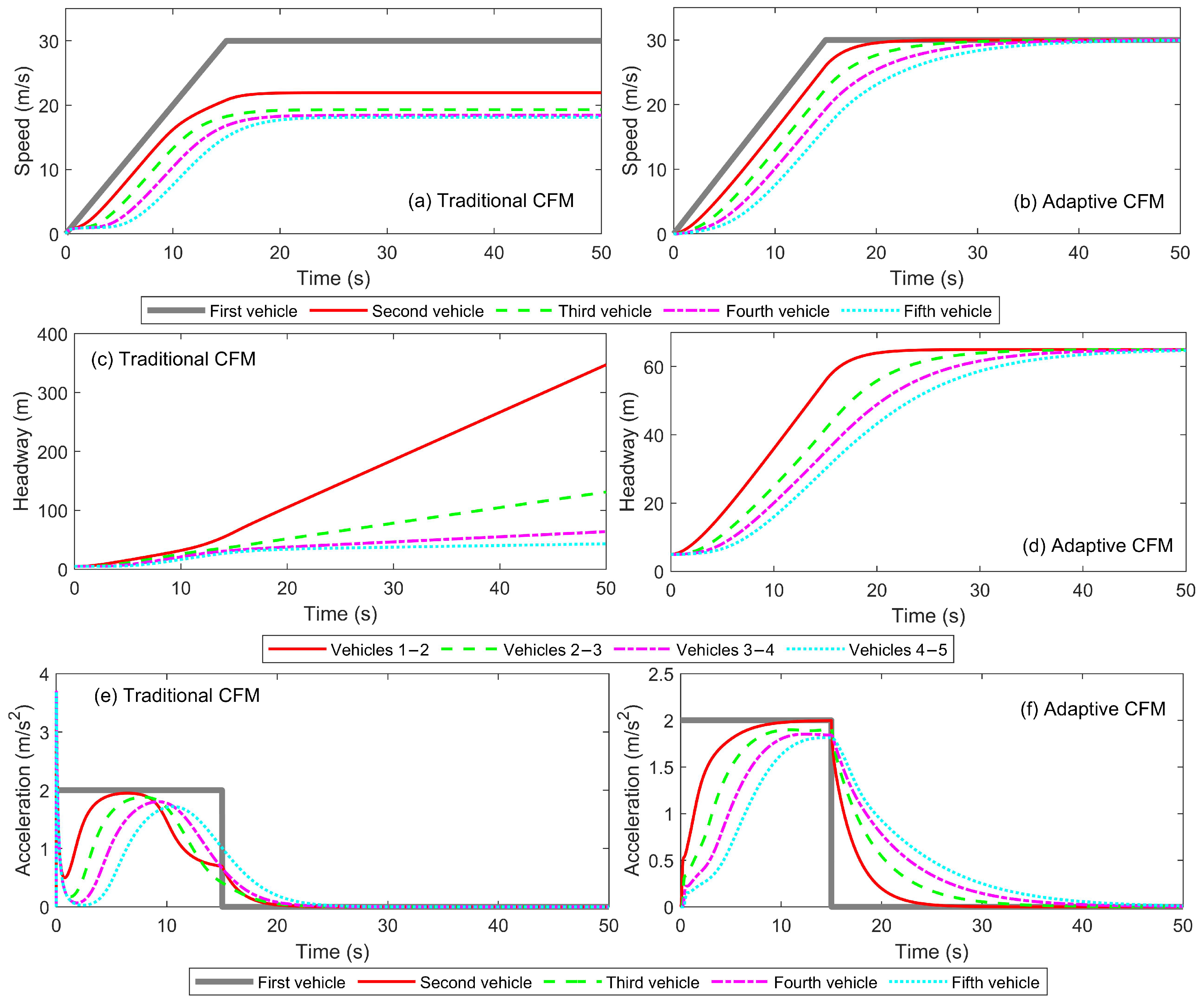
In this study, a comparison between the traditional CFM and the adaptive CFM was conducted to validate the significant advantages of the adaptive CFM Due to the static limitations on maximum speed in the traditional CFM, the following vehicles exhibit noticeable lag and fluctuations when responding to acceleration changes of the leading vehicle. This results in uneven distribution of vehicle speeds and accelerations within the platoon, increasing the instability of the headway and affecting the smoothness and efficiency of traffic flow. In contrast, the adaptive CFM, utilizing the UKF algorithm, dynamically adjusts the maximum speed of each vehicle based on the real-time state of the leading vehicle. This enables smoother speed and acceleration responses for the following vehicles, significantly reducing sudden changes in acceleration and fluctuations in headway during the acceleration process. Experimental results show that the adaptive CFM outperforms the traditional CFM in terms of speed synchronization, headway stability, and acceleration smoothness, effectively improving the platoon stability and traffic flow efficiency. The introduction of the adaptive CFM provides strong support for the realization of a more efficient and safer intelligent transportation system, with broad application prospects.

Looking forward, several research directions may further enhance the applicability and robustness of the proposed approach. First, since the current validation is limited to theoretical simulations, future studies should incorporate empirical traffic data, leverage advanced simulation platforms such as SUMO or VISSIM, explore the development of hybrid models, and consider hardware-in-the-loop testing to strengthen real-world applicability. Second, while the proposed CFM assumes real-time data from surrounding vehicles, typically via V2V communication, the deployment of V2V technology is still in progress. Ongoing advancements in 5G and connected vehicle technologies are accelerating this process. Even in the absence of comprehensive V2V coverage, sensors such as radar, LiDAR, and cameras, combined with machine learning, can provide comparable real-time data to support adaptive CFMs. Finally, integrating reinforcement learning, model predictive control, or fuzzy logic with the proposed UKF-based model represents a promising avenue for future work, potentially further enhancing adaptability and robustness for platoon control under complex and uncertain traffic conditions.