Dual Modal Intelligent Optimization BP Neural Network Model Integrating Aquila Optimizer and African Vulture Optimization Algorithm and Its Application in Lithium-Ion Battery SOH Prediction

Abstract

To enhance the accuracy and robustness of lithium-ion battery state-of-health (SOH) prediction, this study proposes a dual-mode intelligent optimization BP neural network model (AO–AVOA–BP) which integrates the Aquila Optimizer (AO) and the African Vulture Optimization Algorithm (AVOA). The model leverages the global search capabilities of AO and the local exploitation strengths of AVOA to achieve efficient and collaborative optimization of network parameters. In terms of feature construction, eight key health indicators are extracted from voltage, current, and temperature signals during the charging phase, and the optimal input set is selected using gray relational analysis. Experimental results demonstrate that the AO–AVOA–BP model significantly outperforms traditional BP and other improved models on both the NASA and CALCE datasets, with MAE, RMSE, and MAPE maintained within 0.0087, 0.0115, and 1.095%, respectively, indicating outstanding prediction accuracy and strong generalization performance. The proposed method demonstrates strong generalization capability and engineering adaptability, providing reliable support for lifetime prediction and safety warning in battery management systems (BMS). Moreover, it shows great potential for wide application in the health management of electric vehicles and energy storage systems.

1. Introduction

Lithium-ion batteries have been widely adopted in various fields such as electric vehicles and renewable energy storage systems due to their high energy density, long cycle life, and excellent stability [1,2]. They have become a key energy carrier in advancing the transition of the energy structure and promoting the sustainable development of green transportation [3,4]. However, during repeated charge–discharge cycles, irreversible aging phenomena such as active material degradation and electrolyte decomposition occur, leading to capacity fade and increased internal impedance [5], which directly impacts the reliability of the battery’s state of health (SOH) [6]. As a critical indicator representing the remaining useful life of a battery, accurate SOH prediction is essential for ensuring the safe operation of battery systems and optimizing maintenance strategies [7,8].

Existing SOH prediction methods can be broadly classified into three categories:

(1)

Traditional machine learning methods. These approaches mainly rely on manually constructed features combined with statistical learning models for prediction. For example, support vector machines, Gaussian filters, and random forests have been widely applied to SOH modeling. However, in scenarios involving high-dimensional and complex data, these methods are often constrained by limited feature representation capability and high sensitivity to data noise [9,10]. In addition, some studies have attempted to enhance prediction performance by integrating mechanistic modeling with statistical learning [11]. For instance, Bian et al. [12] combined the open-circuit voltage model with incremental capacity analysis and proposed a hybrid modeling method adapted to temperature variations; Hosseininasab et al. [13] employed a fractional-order model to jointly estimate internal resistance and capacity degradation; Chen et al. [14] introduced electrolyte dynamics into the single-particle model, and together with Padé approximation and least squares estimation, they ultimately achieved high-accuracy lifetime prediction through a mapping particle filter (MPF). Although these methods exhibit a certain degree of interpretability, their accuracy and adaptability remain limited in practical applications due to the complexity of electrochemical reactions and the diversity of operating conditions [15,16,17].

(2)

Deep learning methods. With advances in computational power, deep learning has gradually become the mainstream direction for SOH prediction. By leveraging end-to-end feature learning, it demonstrates strong nonlinear modeling and feature extraction capabilities [16,17]. For example, Li et al. [18] proposed a prediction framework combining convolutional neural networks with online transfer learning, which significantly reduced prediction errors across multiple datasets; Tong et al. [19] employed an Adaboost–grey wolf optimization BP neural network, effectively improving SOH prediction accuracy; Gong et al. [20] developed a hybrid network based on an encoder–decoder architecture, where the BP neural network served as the decoder to enhance interpretability; Lei et al. [21] proposed a method combining broadband electrochemical impedance spectroscopy (EIS) rapid detection with ASO-optimized BP networks, achieving efficient and accurate lifetime prediction with a total time reduction of 82.9% and prediction errors controlled within 1.1 cycles; Ma et al. [22] introduced an IPSO-BPNN algorithm based on a mutation particle swarm optimizer and exponential decay learning rate, which leveraged health indicators from the charging stage to achieve highly accurate SOH and RUL prediction, with a maximum error of only 0.78% and an average error of 1.01%, significantly outperforming standard BPNN. Despite their strong advantages, deep learning methods generally require large-scale datasets for training and are prone to challenges associated with parameter initialization and local convergence.

(3)

Hybrid optimization methods. To address the limitations of BP neural networks in terms of local minima and parameter sensitivity, researchers have introduced metaheuristic algorithms to optimize weights and thresholds, thereby improving prediction accuracy and convergence stability. For example, Farong et al. [23] integrated maximum information coefficient (MIC) feature selection with the Golden Jackal Optimization (GJO) algorithm, which significantly enhanced the accuracy and convergence speed of BP networks, achieving improvements of 22.85% and 50% in MAE and convergence efficiency, respectively, compared with traditional GA-BP and SA-BP models. Furthermore, the African Vulture Optimization Algorithm (AVOA), a recently proposed swarm intelligence optimization method inspired by vulture foraging behavior, exhibits strong local exploitation capability. However, it suffers from insufficient exploration ability and unstable convergence speed, often leading to local optima [24]. To overcome these drawbacks, several studies have attempted to integrate multiple mechanisms for performance enhancement: Liu et al. [25] combined quasi-oppositional learning with differential evolution optimization; Alizadeh et al. [26] fused the salp swarm optimization mechanism with AVOA; and Mostafa et al. [27] introduced the Archimedes optimization concept to strengthen the global–local balance. Duan et al. [28] employed an improved whale optimization algorithm (IWOA) to optimize the hyperparameters of the variable forgetting factor online sequential extreme learning machine (VFOS-ELM), while integrating extremely randomized trees (ERT) to extract features highly correlated with capacity. This approach effectively reduced model complexity and simultaneously improved SOH prediction accuracy to above 99.9%. These studies collectively demonstrate that hybrid metaheuristic optimization represents an effective approach for improving SOH prediction performance.

However, most existing improvement strategies for AVOA primarily focus on enhancing its local exploitation capability, while paying insufficient attention to the dynamic balance between exploration and exploitation. For example, both differential evolution and Archimedes optimization perform well during the local search phase but remain prone to premature convergence in the global search stage. This indicates that relying solely on AVOA or its variants makes it difficult to achieve global robustness in high-dimensional and complex spaces. In contrast, the recently proposed Aquila Optimizer (AO) demonstrates remarkable global exploration advantages by simulating the multi-stage hunting behavior of eagles, such as high-altitude soaring, rapid diving, and gradual approaching. Its multi-strategy switching mechanism enables full expansion of the search space during the early stage and gradual convergence toward the optimal solution in the later stage. Therefore, AO and AVOA exhibit natural complementarity in their search mechanisms: the former emphasizes global exploration, whereas the latter focuses on local exploitation. Their combination can theoretically realize a dynamic “global–local” bimodal synergy.

Despite the extensive efforts in existing studies to combine various intelligent optimization algorithms (such as GJO, ASO, and IPSO) with BP neural networks to enhance the accuracy and efficiency of SOH and RUL prediction, two major limitations remain. First, most hybrid strategies primarily emphasize improving the local exploitation capability, which makes them prone to premature convergence in high-dimensional and complex spaces. Second, the exploration–exploitation mechanism in the optimization process lacks dynamic cooperative scheduling, making it difficult to balance global search ability and convergence speed simultaneously. To address these issues, this study proposes a dual-modal optimization mechanism that integrates two metaheuristic algorithms with complementary characteristics—AO and AVOA—to construct a cooperative optimization framework with both global exploration capability and local exploitation efficiency. Specifically, the broad search strategy of AO is organically combined with the multi-mechanism exploitation strategy of AVOA, thereby forming a dual-modal cooperative evolutionary mechanism at the algorithmic level. This mechanism adaptively adjusts the balance between exploration and exploitation according to the population fitness, enabling efficient optimization of the weights and biases of BP neural networks.

This method not only addresses the limitations of traditional hybrid optimization that overly rely on local exploitation, but also achieves global–local collaborative optimization through a bimodal dynamic scheduling mechanism, thereby effectively tackling the two major challenges described above.

Consequently, this paper presents a BP neural network-based SOH prediction model optimized by the AO–AVOA dual-modal intelligent algorithm. The model first analyzes operational data during the battery charging phase and selects key health indicators using gray relational analysis to construct the feature input set. Then, the AO–AVOA is used to optimize the BP network parameters. Finally, experiments are conducted on publicly available NASA and CALCE datasets. The results show that the proposed model outperforms benchmark models in terms of prediction accuracy, generalization ability, and stability, indicating strong potential for practical engineering applications.

2. Battery Aging Data and Health Indicator Extraction

2.1. Battery Aging Data

The battery data used in this study were obtained from two publicly available and widely adopted datasets for battery health management research: one released by the Prognostics Center of Excellence at the National Aeronautics and Space Administration (NASA), and the other by the Center for Advanced Life Cycle Engineering (CALCE) at the University of Maryland. Specifically, this study selects NASA batteries B0005, B0006, B0007, and B0018, as well as CALCE batteries CS2-35, CS2-36, CS2-37, and CS2-38 as research subjects. The NASA dataset, characterized by clearly defined degradation trajectories, is chosen as a representative case for conducting in-depth analysis of charge–discharge characteristics and extracting health indicators, thereby laying the foundation for model development and performance evaluation.

The lithium-ion batteries in the NASA dataset have a nominal capacity of 2.2 Ah and a nominal voltage of 3.7 V. The experiments were conducted at a constant room temperature of 24 °C and included three typical testing protocols: constant current–constant voltage (CC–CV) charging, constant current (CC) discharging, and Electrochemical Impedance Spectroscopy (EIS) measurements. Specifically, during charging, each battery was charged at a constant current of 1.5 A until the voltage reached 4.2 V, after which the protocol switched to constant voltage mode, maintaining 4.2 V until the current decayed to below 20 mA. During the discharge phase, a constant current of 2 A was applied. The discharge cut-off voltages varied by battery: 2.7 V for B0005, 2.5 V for B0006, 2.2 V for B0007, and 2.5 V for B0018. Throughout the experiment, once the actual capacity of a battery declined to 70% of its initial capacity, it was considered to have reached its end of life (EOL), and the test was terminated. This standardized testing protocol provides reliable experimental support and high-quality data for subsequent modeling of battery degradation and remaining useful life prediction.

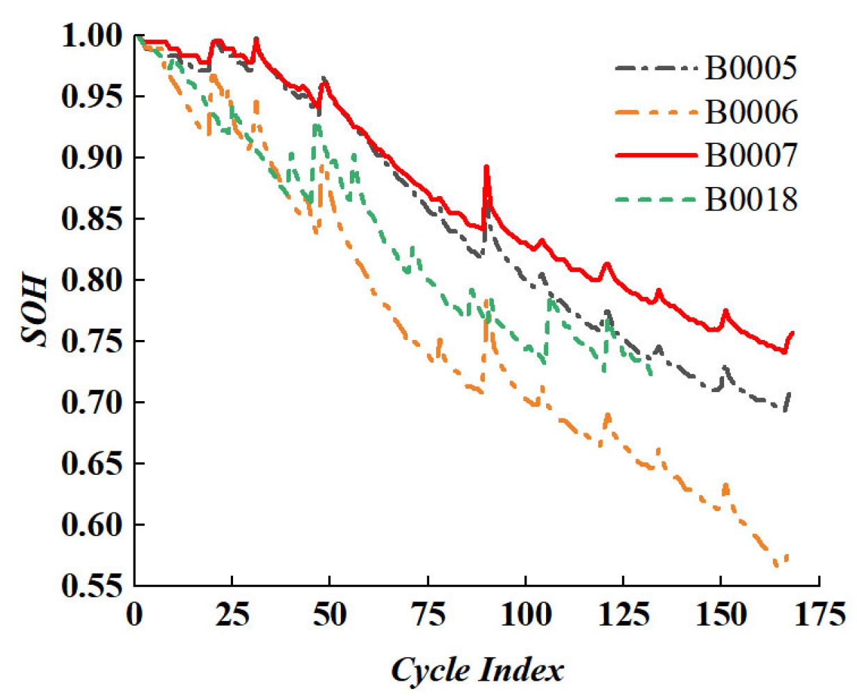
The SOH change curves of the four batteries are shown in Figure 1. It can be seen from Figure 1 that the SOH of the battery shows a downward trend with the increase in the cycle period. The battery SOH in this paper is defined from the perspective of capacity, as shown in Formula (1):

$$SOH={\displaystyle \frac{C_{now}}{C_{rated}}}\times 100\%$$

(1)

$C_{now}$ represents the current maximum capacity of the battery when it is fully filled, and $C_{rated}$ represents the rated capacity of the battery when it leaves the factory.

2.2. Health Indicator Extraction

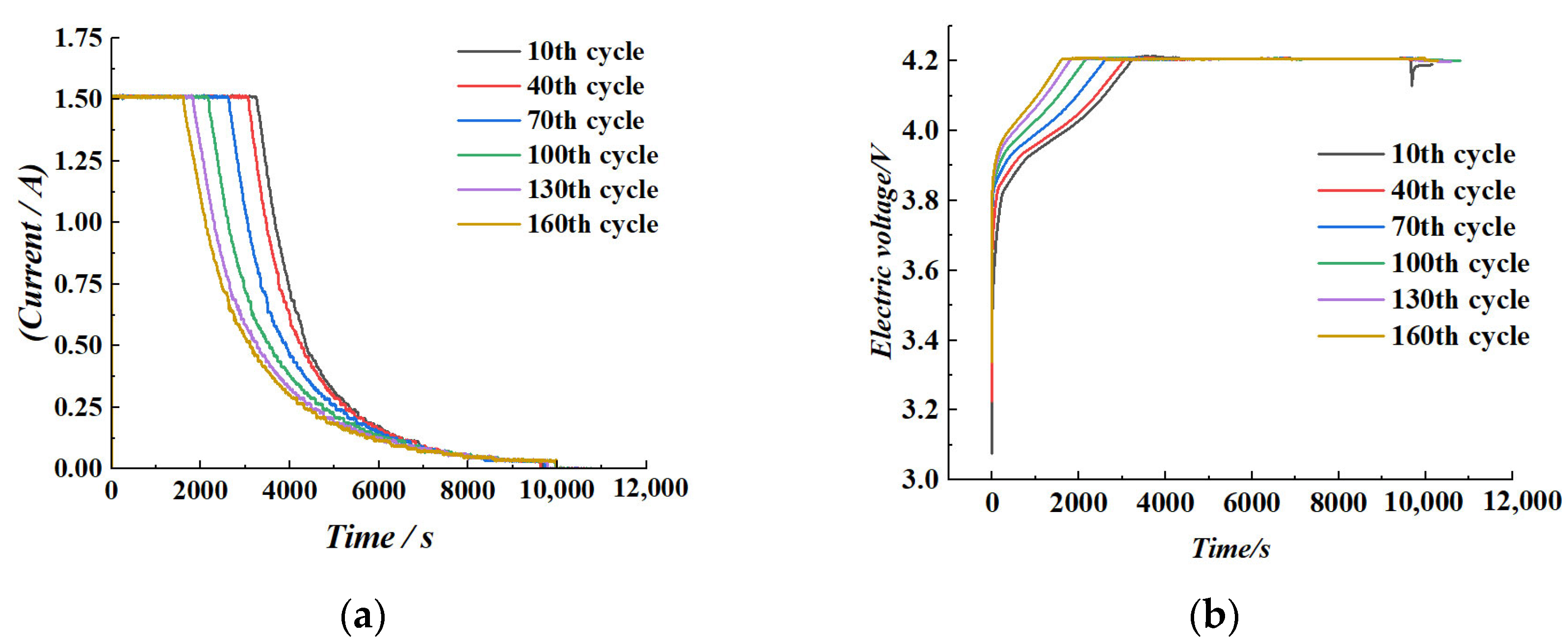
Considering that the discharge process of lithium-ion batteries is often subject to dynamic and variable operating conditions in real-world applications—making precise control challenging—this study prioritizes the use of charging-phase parameters for health indicator extraction, owing to their greater stability and repeatability. This approach is intended to facilitate effective prediction of the battery’s State of Health (SOH). Specifically, this section takes the B0005 battery as a representative case and selects the charging durations during the constant current (CC) and constant voltage (CV) phases in cycles 10, 40, 70, 100, 130, and 160 as analysis features. The results are illustrated in Figure 2a,b. Experimental findings reveal a clear downward trend in the CC charging duration with increasing cycle number, decreasing from an initial 3221 s to 1579 s. In contrast, the CV charging duration exhibits the opposite trend, increasing from approximately 6900 s to about 8700 s. These dynamic changes in charging time reflect the impact of increased internal resistance and enhanced polarization effects on the charging behavior, effectively characterizing the battery’s performance degradation. Therefore, they serve as key features for constructing high-accuracy SOH estimation models.

Figure 3 illustrates the trends of capacity and time during different charging phases of lithium-ion batteries across multiple cycles. As shown in Figure 3a, during the constant current (CC) charging phase, both charging time and charging capacity exhibit a gradual decline as the cycle number increases. Conversely, Figure 3b demonstrates that during the constant voltage (CV) charging phase, both metrics increase progressively with cycling. This pattern reflects the evolving behavior of the battery during aging, revealing how internal property changes influence the charging process.

Based on this observation, this study proposes extracting and constructing composite features from raw signals such as voltage and current to characterize the battery’s State of Health (SOH). Specifically, charging time and capacity during the CC and CV phases are regarded as fundamental health indicators. Additionally, to capture the overall integrity of the charging process, the ratios of the corresponding CC and CV parameters—namely, the CC/CV charging time ratio and CC/CV charging capacity ratio—are introduced as enhanced features. These ratios provide a more comprehensive representation of battery charging behavior and performance degradation trends, thereby providing a more robust basis for SOH modeling and prediction.

In summary, a total of eight health factors are selected as inputs to estimate the state of health (SOH) of lithium-ion batteries, namely: constant-current (CC) charging time (H1), constant-voltage (CV) charging time (H2), CC charging capacity (H3), CV charging capacity (H4), CV discharge time (H5), CV discharge capacity (H6), peak value of the current–capacity curve (H7), and the corresponding voltage at the peak of the current–capacity curve (H8).

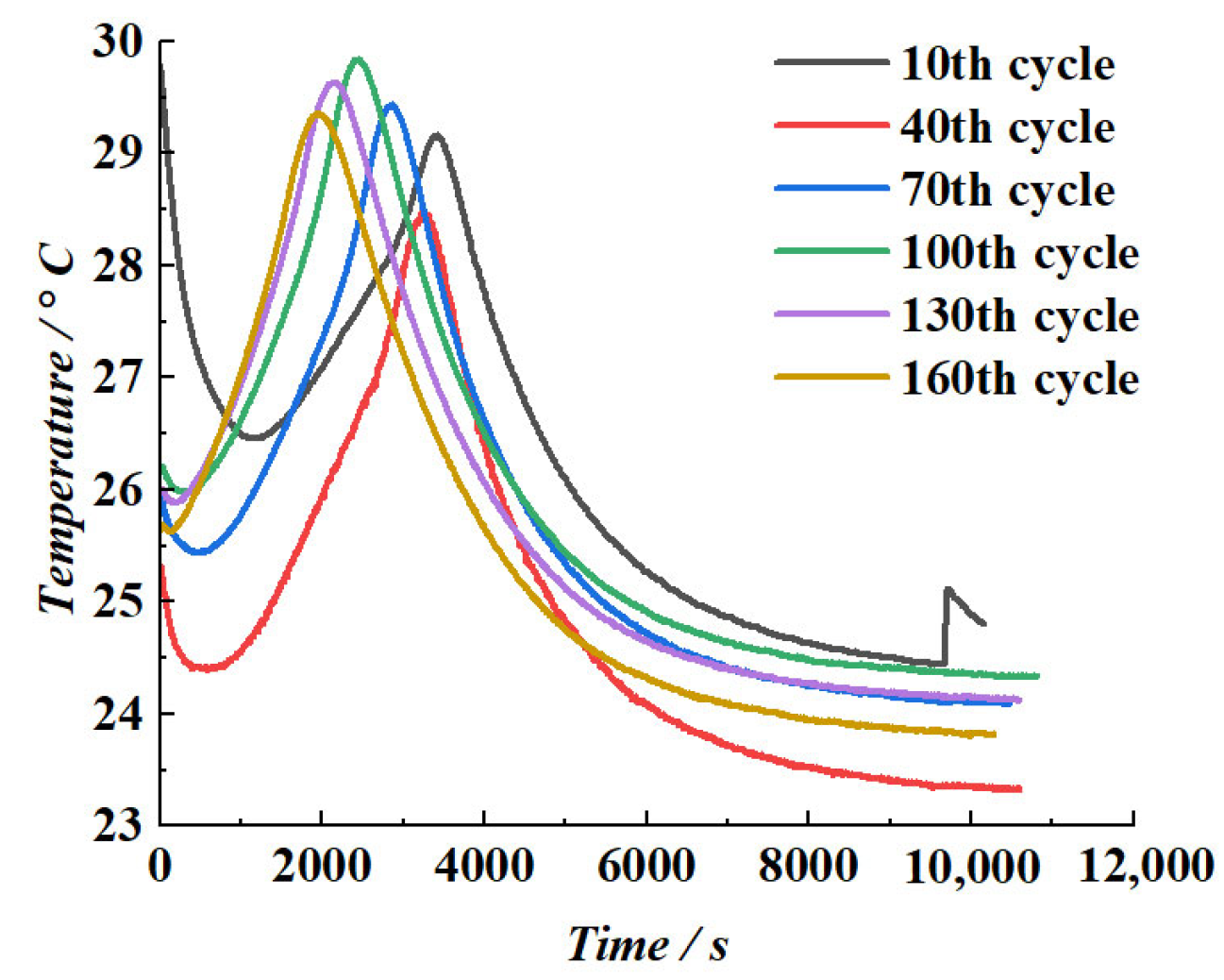
Figure 4 illustrates the temperature variation trends of lithium-ion batteries at different cycle numbers (10th, 40th, 70th, 100th, 130th, and 160th cycles). The results indicate that, within each charging cycle, the battery temperature follows a typical pattern of initially decreasing, then increasing, and ultimately stabilizing. As the cycle number increases, the temperature variations exhibit progressively more distinct patterns, particularly the temperature rise observed during the constant current (CC) charging phase and the average temperature changes during the constant voltage (CV) charging phase. Analyzing these temperature variation patterns further reveals the evolution of the battery’s State of Health (SOH) over the course of cycling.

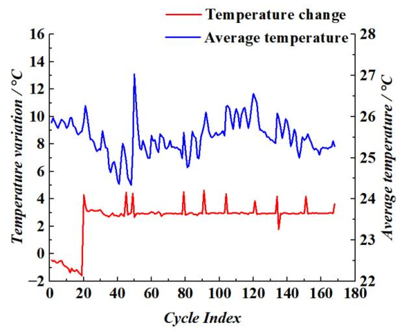
Figure 5 further reveals the variation trends of temperature rise during the constant current (CC) charging phase and the average temperature during the constant voltage (CV) phase across different cycle numbers. Although the evolution of battery temperature does not exhibit a direct linear correlation with capacity degradation, thermal fluctuations are observed during the charge–discharge process due to continuous heat generation from complex internal electrochemical reactions. As an important physical indicator of the battery’s internal dynamic behavior, temperature can indirectly reflect the battery’s State of Health (SOH) to a certain extent. Therefore, incorporating temperature variation characteristics into the SOH estimation framework provides useful supplementary information for monitoring battery degradation and predicting its remaining useful life.

2.3. Correlation Analysis

To evaluate the correlation between the selected health indicators and the battery’s State of Health (SOH), Grey Relation Analysis (GRA) is employed to assess the quality of these feature points. First, the reference sequence and the comparative sequences are defined, where the reference sequence corresponds to the SOH, and the comparative sequences consist of the eight proposed health indicators. Subsequently, the original data are normalized using the initial value method, as shown in Equation (2):

$${\mathrm{x}}_{\mathrm{i}}^{\mathrm{*}}\left(\mathrm{k}\right)={\displaystyle \frac{{\mathrm{x}}_{\mathrm{i}}\left(\mathrm{k}\right)}{{\mathrm{x}}_{\mathrm{i}}\left(1\right)}}$$

(2)

${\mathrm{x}}_{\mathrm{i}}^{\mathrm{*}}\left(\mathrm{k}\right)$ is the dimensionless comparable feature vector, ${\mathrm{x}}_{\mathrm{i}}\left(1\right)$ is the first data of the i th sequence in the original data sequence, and k is the dimension of the vector. Then, the relationship between the comparable feature data and the label data is clarified by calculating the gray correlation coefficient ξ between the comparable feature vector and the label vector, as shown in Formula (3):

$${\mathsf{\xi }}_{\mathrm{i}}\left(\mathrm{k}\right)={\displaystyle \frac{\underset{\mathrm{i}}{\mathrm{m}\mathrm{i}\mathrm{n}}\underset{\mathrm{k}}{\mathrm{m}\mathrm{i}\mathrm{n}}\left|{\mathrm{y}}_{\mathrm{i}}\left(\mathrm{k}\right)-{\mathrm{x}}_{\mathrm{i}}^{\mathrm{*}}\left(\mathrm{k}\right)\right|+\mathsf{\rho }\underset{\mathrm{i}}{\mathrm{m}\mathrm{a}\mathrm{x}}\underset{\mathrm{k}}{\mathrm{m}\mathrm{a}\mathrm{x}}\left|{\mathrm{y}}_{\mathrm{i}}\left(\mathrm{k}\right)-{\mathrm{x}}_{\mathrm{i}}^{\mathrm{*}}\left(\mathrm{k}\right)\right|}{\left|{\mathrm{y}}_{\mathrm{i}}\left(\mathrm{k}\right)-{\mathrm{x}}_{\mathrm{i}}^{\mathrm{*}}\left(\mathrm{k}\right)\right|+\mathsf{\rho }\underset{\mathrm{i}}{\mathrm{m}\mathrm{a}\mathrm{x}}\underset{\mathrm{k}}{\mathrm{m}\mathrm{a}\mathrm{x}}\left|{\mathrm{y}}_{\mathrm{i}}\left(\mathrm{k}\right)-{\mathrm{x}}_{\mathrm{i}}^{\mathrm{*}}\left(\mathrm{k}\right)\right|}}$$

(3)

$\mathsf{\rho }$ is the resolution coefficient, usually 0.5. Finally, the above gray correlation coefficients are weighted and averaged to obtain the gray correlation coefficient ri between the ith feature vector and the label vector, as shown in Formula (4):

$$r_i={\displaystyle \frac{1}{n}}\sum _{k=1}^n{\xi }_i\left(k\right)$$

(4)

The grey relational coefficient is used to quantitatively evaluate the strength of association between each feature vector and the reference vector. A coefficient value closer to 1 indicates a stronger correlation, while a value farther from 1 suggests a weaker correlation. The gray relational coefficients between the health factors and SOH are presented in

Table 1. Grey correlation coefficient between different health factors and SOH.

Battery Number	H1	H2	H3	H4	H5	H6	H7	H8
B0005	0.9171	0.8213	0.9171	0.8309	0.9800	0.9803	0.9225	0.8843
B0006	0.9068	0.7971	0.9068	0.7894	0.9713	0.9713	0.9128	0.8755
B0007	0.9324	0.8192	0.9324	0.8555	0.9838	0.9843	0.9306	0.8829
B0018	0.9557	0.8965	0.9557	0.8912	0.9889	0.9886	0.9126	0.9201
CS2-35	0.9218	0.7250	0.9217	0.7388	0.9552	0.9498	0.7531	0.8675
CS2-36	0.9511	0.7494	0.9511	0.7656	0.9896	0.9801	0.7618	0.8591
CS2-37	0.9521	0.7580	0.9521	0.7715	0.9901	0.9820	0.7867	0.8742
CS2-38	0.9500	0.7799	0.9501	0.7844	0.9878	0.9808	0.7639	0.8713

. As shown in Table 1, most of the gray relational grades exceed 0.7, indicating that the selected health factors H1–H8 exhibit significant correlations with the SOH index and can therefore be employed as inputs to the SOH estimation model. Specifically, health factors such as H1, H3, H5, and H6 demonstrate particularly strong correlations with SOH, with most coefficients approaching or exceeding 0.95, highlighting their superior capability in characterizing battery health status. In contrast, although factors such as H2, H4, and H8 exhibit relatively lower correlations, their values remain at a high level, suggesting that they also exert a non-negligible influence on SOH variation.

Although the results of the grey relational analysis demonstrate that all selected health indicators exhibit significant correlations with SOH, this does not imply that the features are completely independent. Several indicators are derived from the same charging or discharging stages, leading to potential mechanistic coupling and statistical correlations. For instance, H1 and H3 both directly reflect the electrochemical behavior during the constant-current phase and may therefore contain partially overlapping information. Similarly, H7 and H8 may be jointly influenced by polarization effects, thereby introducing a certain degree of redundancy into the input feature space. Such redundancy could reduce the model’s effective degrees of freedom and compromise its generalization capability. To ensure the completeness of the input information, however, all health indicators are retained at the current stage as inputs to the SOH estimation model.

3. Construction of the Lithium-Ion Battery SOH Prediction Model

3.1. Improved AO-AVOA Dual-Modal Intelligent Optimization Algorithm

The Aquila Optimizer (AO) is a population-based metaheuristic optimization algorithm proposed by Abualigah et al. [29] in 2021. In the AO algorithm, each Aquila represents a potential solution, while the prey symbolizes the global optimum. Similarly to many other intelligent optimization algorithms, the initial population in the AO algorithm is generated according to Equation (5):

$$X_i=rand\times \left(UB-LB\right)+LB,i=\mathrm{1,2},\dots ,N$$

(5)

${\mathrm{X}}_{\mathrm{i}}$ denotes the position of the ith solution, rand is a random number between 0 and 1, and UB and LB are the upper and lower bounds of the expected problem, respectively.

The algorithm solves the optimization problem by simulating the predatory behavior of the eagle in nature. The optimization process is divided into four discrete stages to simulate the gradual transition from global search to local hunting.

(1)

Expanded exploration stage

In the first stage, the algorithm focuses on the extensive exploration of the search space to locate the location of potential prey, thereby enhancing the global search ability. The behavior of this stage can be described by the corresponding mathematical model, which lays the foundation for the subsequent optimization process. The mathematical model is as follows:

$${\mathrm{X}}_1\left(\mathrm{t}+1\right)={\mathrm{X}}_{\mathrm{b}\mathrm{e}\mathrm{s}\mathrm{t}}\left(\mathrm{t}\right)\times \left(1-{\displaystyle \frac{\mathrm{t}}{\mathrm{T}}}\right)+\left({\mathrm{X}}_{\mathrm{m}}\left(\mathrm{t}\right)-{\mathrm{X}}_{\mathrm{b}\mathrm{e}\mathrm{s}\mathrm{t}}\left(\mathrm{t}\right)\times \mathrm{r}\mathrm{a}\mathrm{n}\mathrm{d}\right)$$

(6)

$$X_m\left(t\right)={\displaystyle \frac{1}{N}}\sum _{k=1}^N{X}_i\left(t\right)$$

(7)

${\mathrm{X}}_{\mathrm{m}}\left(\mathrm{t}\right)$ represents the average position of all individuals in the current population, ${\mathrm{X}}_{\mathrm{b}\mathrm{e}\mathrm{s}\mathrm{t}}\left(\mathrm{t}\right)$ represents the best position achieved so far, N is the overall size, rand is a random number between 0 and 1, t and T are the current iteration and the maximum number of iterations, respectively.

(2)

Reduce the exploration stage

The second stage is narrow exploration, representing a short glide to attack prey. The position update formula of the eagle is as follows:

$${\mathrm{X}}_2\left(\mathrm{t}+1\right)={\mathrm{X}}_{\mathrm{b}\mathrm{e}\mathrm{s}\mathrm{t}}\left(\mathrm{t}\right)\times \mathrm{L}\mathrm{F}\left(\mathrm{D}\right)+{\mathrm{X}}_{\mathrm{R}}\left(\mathrm{t}\right)+\left(\mathrm{y}-\mathrm{x}\right)\times \mathrm{r}\mathrm{a}\mathrm{n}\mathrm{d})$$

(8)

D is the dimension space, ${\mathrm{X}}_{\mathrm{R}}\left(\mathrm{t}\right)$ represents the random position of the Aquila, $\mathrm{L}\mathrm{F}\left(\mathrm{D}\right)$ represents the Levy flight function, x and y represent the spiral shape of the algorithm in the search space, respectively. The definition is as follows:

$$\mathrm{L}\mathrm{F}\left(\mathrm{D}\right)=\mathrm{s}\times {\displaystyle \frac{\mu \times \sigma }{{\left|\nu \right|}^{\frac{1}{\beta }}}}, \sigma ={\displaystyle \frac{\mathsf{\gamma }\left(1+\beta \right)\times \mathrm{s}\mathrm{i}\mathrm{n}\left(\frac{\mathsf{\pi }\beta }{2}\right)}{\mathsf{\gamma }\left(\frac{1+\beta }{2}\right)\times \beta \times 2^{\left(\frac{\beta -1}{2}\right)}}}$$

(9)

$$\left\{\begin{array}{ll}x=\left(r+0.00565\times D_1\right)\times sin\left(-\omega \times D_1+{\displaystyle \frac{3\pi }{2}}\right)& \\ & \\ y=\left(r+0.00565\times D_1\right)\times cos\left(-\omega \times D_1+{\displaystyle \frac{3\pi }{2}}\right)& \end{array}\right.$$

(10)

s is equal to 0.01, μ and σ are random numbers between 0 and 1, $\beta$ is equal to 1.5, D1 is an integer from 1 to the search space length D, $\mathsf{\omega }$ is equal to 0.005, r is the number of search cycles between 1 and 20.

(3)

Expand the development stage

The third stage, expand the development, involves a vertical landing preliminary attack of prey. This stage is expressed by mathematical formula:

$$X_3\left(t+1\right)=\left(X_{best}\left(t\right)-X_m\left(t\right)\right)\times \alpha -rand+\left(\left(UB-LB\right)\times rand+LB\right)\times \delta$$

(11)

UB and LB denote the upper and lower bounds of the target problem, respectively, while α and δ are exploration adjustment parameters, both set to 0.1.

(4)

Reduce the development stage

The fourth stage, reduce development, involves moving and catching prey. The mathematical model of this behavior is as follows:

$$\left\{\begin{array}{ll}{X}_4\left(t+1\right)=QF\times X_{bact}\left(t\right)-\left(G_1\times X\left(t\right)\times rand\right)-G_2\times LF\left(D\right)+rand\times G_1& \\ QF\left(t\right)=t^{{\displaystyle \frac{2\times tand-1}{{\left(1-T\right)}^2}}},G_1=2\times rand-1,G_2=2\times \left(1-{\displaystyle \frac{t}{T}}\right)& \end{array}\right.$$

(12)

QF represents the quality function used to balance the search strategy, G1 represents the motion parameters when tracking the prey, and G2 represents the flight slope when chasing the prey.

The African Vulture Optimization Algorithm (AVOA), proposed by Abdollahzadeh et al. [30] in 2021, is a novel swarm intelligence-based metaheuristic optimization method. This algorithm simulates the behavioral characteristics of African vultures during their foraging process, including food-searching strategies and variations in flight trajectories, to solve complex optimization problems. Similarly to AO, AVOA also divides the entire optimization process into four distinct stages, gradually driving the convergence of solutions.

(1)

Identification of the Best Vulture Individual

In the initial stage, the algorithm first identifies the vulture individual with the best performance in the current population to provide a guiding direction for subsequent searches. The corresponding mathematical model formalizes the behavior of this stage:

$$R\left(i\right)=\left\{\begin{array}{lllll}{BestVuture}_1& if& p_i=L_1& & \\ {BestVuture}_2& if& p_i=L_2& & \end{array}\right.$$

(13)

R(i) denotes the position of the best vulture. BestVulture₁ and BestVulture₂ represent the best and the second-best vultures, respectively. L₁ and L₂ are parameters in the range [0, 1] that must be initialized before the search operation, with the constraint that their sum equals 1. The variable p_i denotes the selection probability of the best vulture, which is determined using a fitness-based stochastic selection mechanism:

$$p_i={\displaystyle \frac{F_i}{\sum _{i=1}^n{F}_i}}$$

(14)

(2)

Vultures’ hunger index calculation

In the second stage, the starvation index of vultures is calculated, and its mathematical expression is:

$$\left\{\begin{array}{ll}F=\left(2\times ran{d}_1+1\right)\times z\times \left(1-{\displaystyle \frac{{iter}_i}{max\_iter}}\right)+a& \\ t=h\times \left({sin}^{\omega }\left({\displaystyle \frac{\pi }{2}}\times {\displaystyle \frac{{iter}_i}{max\_iter}}\right)+cos\left({\displaystyle \frac{\pi }{2}}\times {\displaystyle \frac{{iter}_i}{max\_iter}}\right)-1\right)& \end{array}\right.$$

(15)

F represents the hunger index of a vulture. The variable ${\mathrm{i}\mathrm{t}\mathrm{e}\mathrm{r}}_{\mathrm{i}}$ denotes the current iteration number, while $\mathrm{m}\mathrm{a}\mathrm{x}\_\mathrm{i}\mathrm{t}\mathrm{e}\mathrm{r}$ refers to the maximum number of iterations. rand₁, z, and h are random variables, with rand₁ ∈ (0, 1), z ∈ (−1, 1), and h ∈ (−2, 2). The parameter ω is a constant predefined before the optimization process begins, with a value set to 2.5.

(3)

Exploration stage

When |F| ≥ 1, the vulture looks for food in different regions, and the algorithm enters the exploration stage. Its mathematical expression is:

$$P\left(i+1\right)=\left\{\begin{array}{ll}R\left(i\right)-\mid X\times R\left(i\right)-P\left(i\right)\mid \times F& P_1\ge ran{d}_{P_1}\\ R\left(i\right)-F+ran{d}_2\left(\left(ub-lb\right)ran{d}_3+lb\right)& P_1<ran{d}_{P_1}\end{array}\right.$$

(16)

P(i) is the position of the vulture, P(i + 1) is the position of the vulture at the next iteration, X = 2 × rand is the coefficient that increases the random motion of the vulture, rand2, rand3 ∈ (0,1) are random values, ub and lb are the upper and lower bounds of the expected problem, respectively.

(4)

Development stage

When |F| < 1, the AVOA enters the exploitation phase. Specifically, when |F| ∈ (0.5, 1), the algorithm proceeds to the first stage of the exploitation phase. If P₂ > rand_P2, a slow encircling strategy is adopted. The corresponding mathematical expression is as follows:

$$\begin{array}{lll}\mathrm{P}\left(\mathrm{i}+1\right)=\mid \mathrm{X}\times \mathrm{R}\left(\mathrm{i}\right)-\mathrm{P}\left(\mathrm{i}\right)\mid \times \left(\mathrm{F}+\mathrm{r}\mathrm{a}\mathrm{n}{\mathrm{d}}_4\right)-\mathrm{d}\left(\mathrm{t}\right)& \mathrm{}& \mathrm{}\\ \mathrm{d}\left(\mathrm{t}\right)=\mathrm{R}\left(\mathrm{i}\right)-\mathrm{P}\left(\mathrm{i}\right)& \mathrm{}& \end{array}$$

(17)

${\mathrm{P}}_2<\mathrm{r}\mathrm{a}\mathrm{n}{\mathrm{d}}_{{\mathrm{p}}_2}$, rotational flight strategy is executed, and its mathematical formulation is given as follows:

$$\left\{\begin{array}{ll}& \\ P\left(i+1\right)=R\left(i\right)-\left(S_1+S_2\right)& \\ & \\ S_1=R\left(i\right)\times \left({\displaystyle \frac{ran{d}_5\times P\left(i\right)}{2\pi }}\right)\times cos\left(P\left(i\right)\right)& \\ & \\ S_2=R\left(i\right)\times \left({\displaystyle \frac{ran{d}_5\times P\left(i\right)}{2\pi }}\right)\times sin\left(P\left(i\right)\right)& \end{array}\right.$$

(18)

where $S_1$ denotes the horizontal (x-axis) component of the rotational flight, and ${\mathrm{S}}_2$ denotes the vertical (y-axis) component of the rotational flight.

When |F| ∈ (0, 0.5), the algorithm enters the second stage of the exploitation phase. If ${\mathrm{P}}_3\ge \mathrm{r}\mathrm{a}\mathrm{n}{\mathrm{d}}_{{\mathrm{p}}_3}$, multiple vultures gather around the food source. The positional behavior of this action is mathematically expressed as:

$$\left\{\begin{array}{lll}P\left(i+1\right)={\displaystyle \frac{A_1+A_2}{2}}& & \\ & & \\ A_{\mathrm{1,2}}=Best{Vuture}_{\mathrm{1,2}}\left(i\right)-{\displaystyle \frac{Best{Vuture}_{\mathrm{1,2}}\left(i\right)-P\left(i\right)}{Best{Vuture}_{\mathrm{1,2}}\left(i\right)-P{\left(i\right)}^2}}\times F& & \end{array}\right.$$

(19)

where $A_1$ and $A_2$ are the position reference quantities calculated based on $Best{Vuture}_1$ and $Best{Vuture}_2$, respectively.

If ${\mathrm{P}}_3<\mathrm{r}\mathrm{a}\mathrm{n}{\mathrm{d}}_{{\mathrm{p}}_3}$, an encircling strategy is implemented. The positional behavior of this action is mathematically formulated as:

$$P\left(i+1\right)=R\left(i\right)-\left|d\left(t\right)\right|\times F\times LF\left(D\right)$$

(20)

Although the AO algorithm demonstrates excellent global exploration capability, its local exploitation performance remains to be improved. In contrast, the AVOA exhibits superior exploitation ability; however, it shows relatively weaker stability in global exploration. Based on the complementary optimization characteristics of these two algorithms, this paper proposes an improved hybrid AO-AVOA optimization algorithm, aiming to enhance solution quality and global search capability. In the proposed algorithm, the position updating mechanism in the exploration phase of the AVOA is modified. Specifically, Equations (6) and (8) are employed to replace the original updating rules, thereby improving population diversity and adaptability in the early stages of the search process. This modification is intended to enhance the overall optimization performance. The corresponding equations are as follows:

$$\begin{array}{l}{X}_i\left(t+1\right)\\ =\left\{\begin{array}{llll}{X}_{best}\left(t\right)\times \left(1-{\displaystyle \frac{t}{T}}\right)+\left(X_m\left(t\right)-X_{best}\left(t\right)\times rand\right)& if rand\le P_1& & \\ & & & \\ X_{best}\left(t\right)\times LF\left(D\right)+X_R\left(t\right)+\left(y-x\right)\times rand)& if rand>P_1& & \end{array}\right.\end{array}$$

(21)

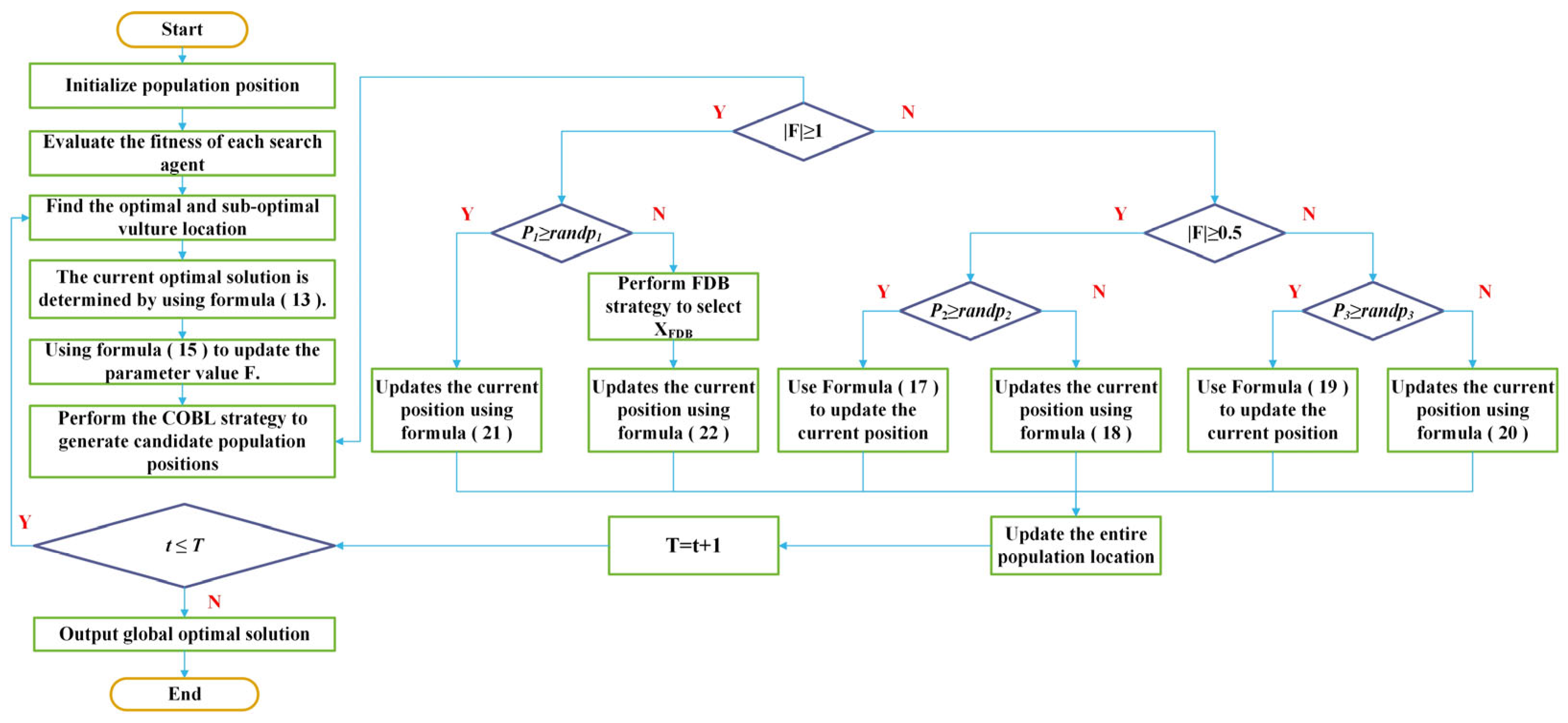
This dual-modal intelligent design scheme establishes a dynamic balance between global exploration and local exploitation by integrating the advantageous features of both algorithms, while significantly enhancing convergence efficiency. To further improve the optimization performance of the baseline hybrid model, two additional strategies are introduced: the Composite Opposition-Based Learning (COBL) strategy and the Fitness-Distance Balance (FDB) strategy. The COBL strategy enhances population diversity by dynamically generating opposite solution space, thereby effectively overcoming potential local convergence bottlenecks during the search process. This strategy is implemented as a preprocessing mechanism prior to each iteration, consistently generating candidate solutions with spatial advantages. Furthermore, according to the updated position Formula (21), the iterative evolution of search agents primarily depends on the current best individual and a randomly selected reference individual. However, the use of randomly selected reference individuals may lead to directional bias in the exploration and exploitation processes, adversely affecting the convergence efficiency of the algorithm. To address this issue and improve search efficiency, the FDB strategy is employed. By dynamically evaluating the fitness contribution of candidate solutions, the strategy establishes a new guidance baseline to replace the randomly selected individual, as illustrated in Equation (22).

$$X_i\left(t+1\right)=X_B\left(t\right)\times LF\left(D\right)+X_{FDB}\left(t\right)+\left(y-x\right)\times rand$$

(22)

In summary, the proposed algorithm achieves notable improvements in three key aspects: solution quality, robustness, and convergence speed. The overall framework of the improved AO-AVOA dual-modal intelligent optimization algorithm is illustrated in Figure 6.

3.2. AO-AVOA-BP Neural Network Model

The Backpropagation (BP) neural network is a representative type of multilayer feedforward neural network, characterized by its dual mechanisms of forward signal propagation and backward error propagation [31]. It demonstrates strong generalization capabilities in addressing complex nonlinear problems. Through the training process, the BP network automatically learns the mapping relationship between input and output variables, making it particularly effective in modeling the nonlinear characteristics of capacity degradation over the full lifecycle of batteries. However, despite its advantages, the BP network exhibits certain limitations in practical applications—most notably, its sensitivity to initial weights and thresholds. This sensitivity increases the risk of the network becoming trapped in local optima, thereby compromising prediction accuracy. To address these shortcomings, this study incorporates the hybrid optimization algorithm AO-AVOA to optimize the initial parameters of the BP neural network. Therefore, an AO-AVOA-BP neural network model is developed for predicting battery State of Health (SOH). The overall modeling framework is illustrated in Figure 7.

It should be noted that although deep learning models such as long short-term memory networks (LSTM) and convolutional neural networks (CNN) have shown outstanding performance in handling time-series degradation data of batteries in recent years, the choice of a BP neural network as the predictive framework in this study is justified for the following reasons. First, by employing gray relational analysis, the time-series data from the battery charge–discharge process have been distilled into several health factors, resulting in highly structured input features; thus, the memory capability of LSTM for long sequences is not required. Second, the BP neural network contains relatively fewer parameters and incurs lower computational costs, making it more suitable for deployment in resource-constrained scenarios such as battery management systems (BMS). Therefore, in this study, the BP network not only ensures prediction accuracy and stability but also provides strong engineering practicality.

4. Experiment

4.1. Experimental Setup

In this study, MATLAB R2023b is employed as the platform for modeling and simulation. Five models are constructed to perform lithium-ion battery State of Health (SOH) prediction and analysis: the standard BP neural network model, PSO-BP model, AO-BP model, AVOA-BP model, and the proposed AO-AVOA-BP model. In the proposed model, the eight health factors extracted earlier in the manuscript are employed as inputs, whereas the output corresponds to the battery’s state of health (SOH). The dataset used for model training and testing is drawn from publicly available battery cycling data provided by NASA and CALCE. Specifically, 70% of the cycling data is used for model training, while the remaining 30% is reserved for testing in order to evaluate the generalization ability and predictive performance of each model. To comprehensively assess the accuracy and stability of the prediction models, three evaluation metrics are adopted: Mean Absolute Error (MAE), Root Mean Square Error (RMSE), and Mean Absolute Percentage Error (MAPE). The corresponding formulas are given in Equations (23)–(25). These metrics reflect the degree of deviation between predicted values and actual measurements from different perspectives, thereby providing an objective basis for evaluating model performance.

$$MAE={\displaystyle \frac{1}{N}}\sum _N^{i=1}|\left(y_i-{\widehat{y}}_i\right)|$$

(23)

$$RMSE=\sqrt{{\displaystyle \frac{1}{N}}\sum _{i=1}^N{\left(y_i-{\widehat{y}}_i\right)}^2}$$

(24)

$$MAPE={\displaystyle \frac{1}{N}}\sum _N^{i=1}\left|{\displaystyle \frac{y_i-{\widehat{y}}_i}{y_i}}\right|\times 100\%$$

(25)

N is the total number of battery cycles; ${\mathrm{y}}_{\mathrm{i}}$ is the true value of the battery SOH; and ${\widehat{\mathrm{y}}}_{\mathrm{i}}$ is the predicted value.

4.2. SOH Prediction Process

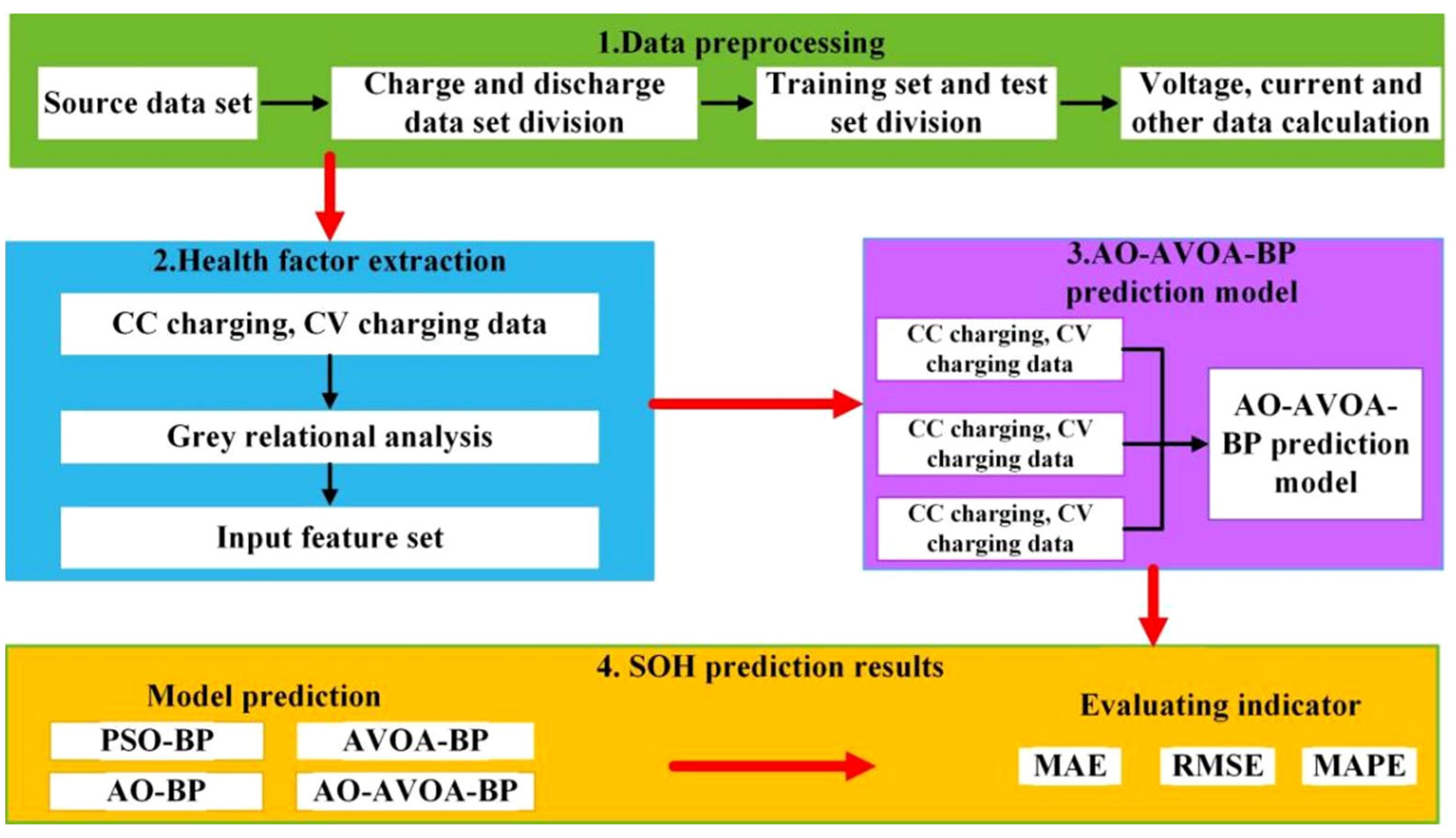
Figure 8 illustrates the overall process of the lithium-ion battery SOH prediction model based on the AO-AVOA-BP neural network. The procedure begins with data preprocessing, during which battery datasets from NASA and CALCE are imported. Key parameters such as voltage, current, and temperature during the charging phase are extracted, and the data are then divided into a training set and a testing set. Next, health factor extraction is conducted. Multidimensional data from the battery charging process is analyzed using the gray relational analysis method to evaluate the correlation among potential health indicators, thereby forming an effective set of input features. Subsequently, the weights and biases of the BP neural network are taken as optimization targets. An improved dual-strategy metaheuristic algorithm, AO-AVOA, is introduced to optimize these parameters, resulting in the construction of a high-precision AO-AVOA-BP prediction model. Finally, the constructed feature set is fed into the prediction model to generate SOH estimates. Model performance is validated using relevant evaluation metrics to ensure the accuracy and practical applicability of the prediction results.

To further elaborate on the datasets used in the SOH prediction process, this study selects four batteries from the NASA dataset—B0005, B0006, B0007, and B0018—as the research subjects. The previously extracted eight health indicators are employed as input features, while the corresponding battery SOH values serve as outputs. For each battery, the first 70% of the cycle data is used as the training set, and the remaining 30% is used as the test set. The AO-AVOA-BP neural network model is adopted for SOH estimation and is compared against baseline models, including the standard BP neural network, PSO-BP, AO-BP, and AVOA-BP neural networks. Compared to the NASA dataset, the CALCE battery dataset offers a more comprehensive characterization of full lifecycle degradation. Specifically, each single-cell battery in the CALCE dataset undergoes approximately five to six times more charge–discharge cycles than those in the NASA dataset, and degradation trajectories are recorded until the capacity falls below 30% of the initial value. According to the Chinese national standard GB/T 34015-2017: Reuse of Automotive Traction Battery—State of Health Determination, the retirement threshold for second-life battery applications is typically set at 80% of the initial capacity. Considering this standard, along with conservative strategies in real-world usage scenarios and the need for consistency with the NASA dataset, this study selects 70% of the initial capacity as the critical threshold for SOH prediction. All SOH prediction tasks are thus performed using data up to the point where the battery capacity declines to 70% of its original value.

5. Results and Discussion

This study aims to systematically evaluate the optimization performance of the proposed improved AO-AVOA dual-strategy intelligent optimization algorithm and its effectiveness in predicting the state of health (SOH) of lithium-ion batteries. First, the convergence behavior and global search capability of the improved AO-AVOA are validated using standard unimodal and multimodal benchmark functions. Subsequently, the algorithm is integrated with a backpropagation (BP) neural network to construct the AO-AVOA-BP prediction model. This model is then applied to SOH estimation tasks based on the NASA and CALCE battery datasets, and experimental results are analyzed accordingly. Finally, by comparing the prediction error metrics under different optimization models, training set proportions, and combinations of health indicators, the model’s accuracy, stability, and generalization ability are comprehensively assessed. These evaluations confirm the effectiveness and practical value of the proposed method for modeling battery health status in real-world scenarios.

5.1. Performance Evaluation of the Improved AO-AVOA Dual-Strategy Intelligent Optimization Algorithm

To verify the performance and feasibility of the proposed AO-AVOA dual-strategy intelligent optimization algorithm, numerical simulation experiments are conducted using a set of standard benchmark functions. Unimodal functions, characterized by a single global optimum, are commonly employed to assess the convergence speed and precision of optimization algorithms. These functions effectively reflect the algorithm’s ability to locate optimal solutions efficiently within smooth search spaces. In contrast, multimodal functions feature more complex search space landscapes with multiple local optima, simulating the non-convexity and multi-solution nature of real-world optimization problems. They are essential for testing an algorithm’s capacity to escape local optima and accurately identify global solutions, serving as key indicators of global search ability and robustness [32]. Accordingly, six representative standard test functions (see

Table 2. Benchmark functions.

Function	Type	Dimension	Hunting Zone	Optimal Value
$F_1\left(x\right)={\displaystyle \sum _{i=1}^D}{x}_i^2$	Singlet	30	[−100, 100]	0
$F_2\left(x\right)=max\{\mid x_i\mid ,1\le i\le D\}$	Singlet	30	[−100, 100]	0
$F_3\left(x\right)={\displaystyle \sum _{i=1}^{D-1}}\left[100{\left(x_{i+1}-x_i^2\right)}^2+{\left(x_i-1\right)}^2\right]$	Singlet	30	[−30, 30]	0
$F_4\left(x\right)={\displaystyle \sum _{i=1}^D}-x_{i}sin\left(\sqrt{\mid x_i\mid }\right)$	Multimodal	30	[−500, 500]	0
$F_5\left(x\right)={\displaystyle \sum _{i=1}^D}\left[x_i^2-10cos\left(2\pi x_i\right)+10\right]$	Multimodal	30	[−5.12, 5.12]	0
$F_6\left(x\right)={\displaystyle \frac{1}{4000}}{\displaystyle \sum _{i=1}^D}{x}_i^2-{\displaystyle \prod _{i=1}^D}cos\left({\displaystyle \frac{x_i}{\sqrt{i}}}\right)+1$	Multimodal	30	[−32, 32]	0

) are selected in this study. These functions span various levels of complexity and search space characteristics, enabling a comprehensive evaluation of the proposed algorithm’s performance across different optimization scenarios.

To validate the performance advantages of the proposed improved AO-AVOA, the original AO algorithm and the AVOA are selected as baseline comparators. In the experimental setup, all algorithms are configured with a maximum of 500 iterations and a population size of 30. Each algorithm is independently executed 30 times on each benchmark function to mitigate the influence of stochastic factors. The performance evaluation primarily relies on two indicators: the mean and standard deviation of fitness values obtained during the optimization process. The mean fitness value reflects the algorithm’s search accuracy, while the standard deviation measures its stability. The mean fitness, calculated as shown in Equation (26), provides a quantitative assessment of the algorithm’s global optimization capability within the solution space.

$$A\nu g={\displaystyle \frac{1}{times}}\sum _{i=1}^{times}{O}_i$$

(26)

times represents the number of times the algorithm runs, ${\mathrm{O}}_{\mathrm{i}}$ representing the fitness value of the ith solution.

When the mean fitness value approaches the theoretical optimum, it indicates that the algorithm possesses high precision and superior convergence performance in global search. To further quantify the distribution characteristics of the solutions, the standard deviation is adopted as a metric for quantitative characterization, as defined in Equation (27).

$$Std=\sqrt{{\displaystyle \frac{1}{times-1}}\sum _{i=1}^{times}{\left(O_i-A\nu g\right)}^2}$$

(27)

Table 3. The optimization results under different test functions.

Function	Algorithm	Average Fitness Value	Standard Deviation
$F_1\left(x\right)$	AO	6.57 × 10−103	3.21 × 10−102
	AVOA	4.00 × 10−288	0
	AO-AVOA	0	0
$F_2\left(x\right)$	AO	3.41 × 10−60	1.35 × 10−59
	AVOA	6.00 × 10−151	3.27 × 10−150
	AO-AVOA	0	0
$F_3\left(x\right)$	AO	5.28 × 10−3	9.52 × 10−3
	AVOA	6.69 × 10−5	6.20 × 10−5
	AO-AVOA	2.44 × 10−7	7.14 × 10−7
$F_4\left(x\right)$	AO	−7.93 × 10−3	3.41 × 10−3
	AVOA	−1.23 × 10−4	6.67 × 10−2
	AO-AVOA	−1.22 × 10−4	1.24 × 10−2
$F_5\left(x\right)$	AO	0	0
	AVOA	0	0
	AO-AVOA	0	0
$F_6\left(x\right)$	AO	2.00 × 10−6	3.16 × 10−6
	AVOA	3.11 × 10−8	4.35 × 10−8
	AO-AVOA	3.70 × 10−9	3.28 × 10−9

presents the optimization results of the improved AO-AVOA compared with other algorithms across various benchmark functions. In the unimodal function tests, the improved AO-AVOA demonstrates outstanding performance in function evaluations, effectively converging to the theoretical optimum. Its convergence speed and accuracy show significant improvements compared with the AO and AVOAs. Although it does not fully reach the global optimum, its solution accuracy is noticeably superior to that of the compared algorithms, confirming its innovative advantages during the local search phase. In the multimodal function tests, all three algorithms are capable of finding the theoretical optimum; however, in function evaluations, the improved AO-AVOA, while not fully converging to the global optimum, still maintains performance superior to the other algorithms. These results indicate that the improved AO-AVOA not only possesses strong global exploration capabilities but is also effective in addressing complex global optimization problems.

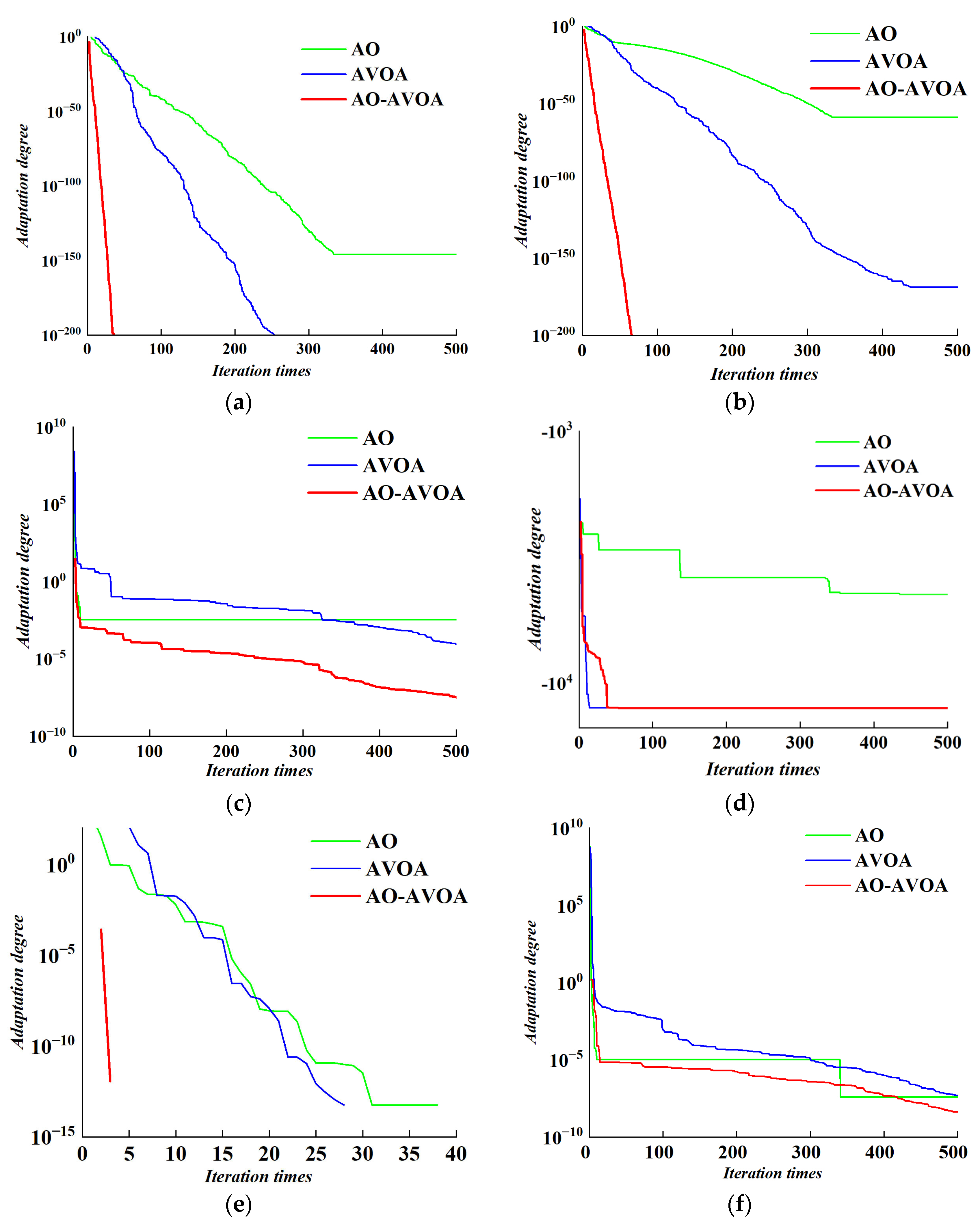
Figure 9 illustrates the convergence curves of the improved AO-AVOA compared with the original AO and AVOAs across several standard benchmark functions. As observed in Figure 8, the improved AO-AVOA consistently demonstrates faster convergence rates and higher convergence accuracy in both unimodal and multimodal optimization tasks. Compared with the original AO and AVOAs, it exhibits stronger global search capabilities during the early stages of optimization and more stable local convergence performance in the later stages. These results further validate the effectiveness of the proposed improvements in enhancing the algorithm’s overall optimization performance. The findings confirm that the improved AO-AVOA not only possesses robust global exploration ability but is also well-suited for solving complex global optimization problems.

In the unimodal function tests, the improved AO-AVOA demonstrated exceptionally high convergence efficiency on functions ${\mathrm{F}}_1\left(\mathrm{x}\right)$ and ${\mathrm{F}}_2\left(\mathrm{x}\right)$, approaching the global optimum almost immediately during the initial phase. This indicates strong search stability and precision. On function ${\mathrm{F}}_3\left(\mathrm{x}\right)$, although the early-stage convergence trajectory resembled that of the AO algorithm, the overall convergence speed was faster. The optimization path gradually aligned with that of AVOA in the later stages, ultimately achieving the highest solution accuracy. This highlights the algorithm’s adaptive capability across different phases of the search process.

In the multimodal function tests, although the improved AO-AVOA did not exactly reach the theoretical optimum on function ${\mathrm{F}}_4\left(\mathrm{x}\right)$, it exhibited a significantly faster convergence rate compared to the other algorithms, indicating effective exploration performance. On function ${\mathrm{F}}_5\left(\mathrm{x}\right)$, the algorithm successfully reached the global optimum within approximately 10 iterations, substantially outperforming the compared methods. On function ${\mathrm{F}}_6\left(\mathrm{x}\right)$, despite a slower start and slight lag behind the AO algorithm, the improved algorithm accelerated in the later stages by effectively escaping local optima, eventually yielding a superior solution. These results validate the robustness and global search potential of the proposed approach in complex multimodal environments.

5.2. Analysis of Model Prediction Results

To verify the SOH prediction capability of the proposed AO-AVOA-BP model, a comparative analysis was conducted with the BP neural network, PSO-BP neural network, AO-BP neural network, and AVOA-BP neural network models. The SOH prediction results and corresponding errors for the NASA and CALCE datasets under different models are shown in Figure 10 and Figure 11, respectively.

As illustrated in Figure 10 and Figure 11, the proposed AO-AVOA-BP model achieved the highest prediction accuracy across all four battery SOH prediction tasks on both the NASA and CALCE datasets, demonstrating a significant advantage in performance. Specifically, the model exhibited minimal error fluctuations, low peak-to-valley differences, and a notably low frequency of outliers. These characteristics indicate strong stability, generalization capability, and robustness across multiple sets of battery degradation data. This superior performance can be primarily attributed to the optimized design of the algorithmic framework. The AO algorithm provides effective global search capabilities, reducing the likelihood of the parameter training process becoming trapped in local optima. The AVOA component enhances dynamic adaptability to non-stationary degradation patterns through its adaptive perturbation mechanism. Meanwhile, the BP neural network offers powerful nonlinear mapping capabilities, enabling it to accurately capture the degradation trend of SOH. The synergy among these three components significantly enhances the model’s capacity for modeling complex electrochemical degradation behavior and ensures high prediction stability.

It is noteworthy that during the 91st cycle test of the CS2-36 battery, the AO-AVOA-BP model exhibited a relatively large local prediction error. However, the model was able to respond promptly and autonomously correct the deviation, allowing the prediction curve to quickly return to a reasonable trajectory and maintain overall accuracy in the subsequent cycles. This indicates that the model not only possesses strong initial prediction capability but also demonstrates robust dynamic recovery and error-suppression mechanisms. It can effectively adjust its parameters in response to data disturbances or abrupt degradation behavior, thereby maintaining the continuity and reliability of the prediction results.

In contrast, the AVOA-BP model exhibited larger and more frequent fluctuations in prediction error during SOH estimation. This instability primarily stems from its lack of global optimization capability, making it prone to local optima and leading to suboptimal parameter tuning. Moreover, its limited ability to model nonlinear degradation features results in inadequate generalization performance. Additionally, when confronted with sudden degradation events or anomalous data, the model shows weak adaptive correction capacity, making it difficult to rectify prediction deviations in a timely manner, thereby exacerbating error instability.

To compare the differences in training efficiency and computational cost among various models, this study conducts a comparative analysis of the convergence speed and computational complexity of BP, PSO-BP, AO-BP, AVOA-BP, and the proposed AO-AVOA-BP model. This analysis not only reveals efficiency differences beyond error performance but also provides a reference for evaluating the feasibility and adaptability of the models in practical engineering applications.

Table 4. Comparison of convergence speed, computational complexity, and advantages and disadvantages of prediction models.

Model	Convergence Rate	Computational Complexity	Advantage	Limitation
BP	Slower, prone to getting stuck in local minima	$\mathrm{O} (\mathrm{n}\cdot \mathrm{d})$	Simple structure, high computing efficiency	Sensitive to initial weights, insufficient convergence performance
PSO-BP	Moderate, convergence speed superior to BP	$\mathrm{O} (\mathrm{n}\cdot \mathrm{d}\cdot \mathrm{T})$	With global search capabilities, it can alleviate the problem of local optimization.	Too many parameters can easily lead to premature convergence.
AO-BP	Moderate, convergence speed faster than PSO-BP	$\mathrm{O} (\mathrm{n}\cdot \mathrm{d}\cdot \mathrm{T})$	Balance exploration and exploitation capabilities to improve global optimization results.	Convergence stability is greatly affected by parameter adjustment.
AVOA-BP	Faster, with a significant reduction in the number of iterations.	$\mathrm{O} (\mathrm{n}\cdot \mathrm{d}\cdot \mathrm{T})$	The adaptive mechanism improves convergence speed and stability.	Unstable performance with some complex datasets
AO-AVOA-BP	Fastest, best overall convergence speed	$\mathrm{O} (\mathrm{n}\cdot \mathrm{d}\cdot \mathrm{T})$	Combining two optimization strategies, it has both global exploration and local development capabilities.	The algorithm structure is complex and computationally expensive.

presents a systematic comparison of the convergence speed, computational complexity, and respective advantages and disadvantages of the different methods, where n denotes the population size, d represents the problem dimension, and T refers to the number of iterations.

As shown in Table 4, different methods exhibit notable differences in convergence efficiency and computational complexity. The traditional BP model has relatively low computational cost but suffers from slow convergence and a tendency to fall into local optima. Single optimization-based approaches (e.g., PSO-BP, AO-BP, and AVOA-BP) achieve improved convergence speed; however, their stability and adaptability remain limited. In contrast, the AO-AVOA-BP model integrates both global search capability and adaptive mechanisms, achieving the fastest overall convergence and greater robustness. Nevertheless, its computational cost is relatively higher, suggesting that a trade-off between accuracy and efficiency should be considered in practical applications.

To comprehensively evaluate the performance of each prediction model in the battery SOH estimation task, this study incorporates multiple evaluation metrics to comparatively analyze their accuracy and stability. By quantifying the prediction errors, the influence of different algorithmic structures on model performance can be further elucidated. Specifically, the SOH prediction results are systematically assessed using Mean Absolute Error (MAE), Root Mean Square Error (RMSE), and Mean Absolute Percentage Error (MAPE). The NASA battery performance metrics are summarized in

Table 5. SOH estimation error evaluation index of NASA battery dataset under different methods.

Battery Number	Model	MAE	MAE Reduction (%) Relative to BP	RMSE	RMSE Reduction (%) Relative to BP	MAPE	MAPE Reduction (%) Relative to BP
B0005	BP	0.0307	-	0.0362	-	4.2993%	-
	PSO-BP	0.0162	47.23%	0.0177	51.10%	2.2607%	47.42%
	AO-BP	0.0108	64.82%	0.0119	67.13%	1.5088%	64.90%
	AVOA-BP	0.0182	40.72%	0.0214	40.88%	2.5507%	40.69%
	AO-AVOA-BP	0.0059	80.78%	0.0065	82.04%	0.8320%	80.64%
B0006	BP	0.0259	-	0.0384	-	4.3661%	-
	PSO-BP	0.0145	44.01%	0.0172	55.21%	2.3964%	45.13%
	AO-BP	0.0124	52.12%	0.0159	58.59%	2.0523%	52.98%
	AVOA-BP	0.0173	33.20%	0.0233	39.32%	2.8911%	33.78%
	AO-AVOA-BP	0.0048	81.47%	0.0057	85.16%	0.7811%	82.11%
B0007	BP	0.0342	-	0.0364	-	4.4671%	-
	PSO-BP	0.0163	52.34%	0.0197	45.88%	2.1474%	51.92%
	AO-BP	0.0133	61.11%	0.0154	57.69%	1.7522%	60.77%
	AVOA-BP	0.0209	38.89%	0.0242	33.52%	2.7433%	38.57%
	AO-AVOA-BP	0.0067	80.41%	0.0071	80.49%	0.8808%	80.29%
B0018	BP	0.0229	-	0.0237	-	3.0630%	-
	PSO-BP	0.0147	35.81%	0.0178	24.89%	1.9811%	35.30%
	AO-BP	0.0113	50.66%	0.0162	31.65%	1.5118%	50.63%
	AVOA-BP	0.0184	19.65%	0.0254	−7.17%	2.4589%	19.71%
	AO-AVOA-BP	0.0062	72.93%	0.0072	69.62%	0.8383%	72.63%

, and the statistical results of the t-test and analysis of variance (ANOVA) are reported in

Table 6. Statistical test results for NASA battery dataset.

Battery Number	Model	t-Test-p	t-Test-t	ANOVA-F	ANOVA-p
B0005	AO-AVOA-BP vs. BP	0.0	8.754	22.672	0
	AO-AVOA-BP vs. AO-BP	0.58864	−0.544
	AO-AVOA-BP vs. AVOA-BP	0.0	−5.33
B0006	AO-AVOA-BP vs. BP	0.00003	4.584	8.432	0.00003
	AO-AVOA-BP vs. AO-BP	0.02816	−2.262
	AO-AVOA-BP vs. AVOA-BP	0.0	17.944
B0007	AO-AVOA-BP vs. BP	0.0	12.476	30.4	0
	AO-AVOA-BP vs. AO-BP	0.00143	−3.38
	AO-AVOA-BP vs. AVOA-BP	0.00002	−4.72
B0018	AO-AVOA-BP vs. BP	0.0731	1.842	7.435	0.00011
	AO-AVOA-BP vs. AO-BP	0.09892	−1.69
	AO-AVOA-BP vs. AVOA-BP	0.00001	−5.124

. The CALCE battery performance metrics are presented in

Table 7. SOH estimation error evaluation index of CALCE battery dataset under different methods.

Battery Number	Model	MAE	MAE Reduction (%) Relative to BP	RMSE	RMSE Reduction (%) Relative to BP	MAPE	MAPE Reduction (%) Relative to BP
CS2-35	BP	0.0348	-	0.0392	-	4.4301%	-
	PSO-BP	0.0238	31.61%	0.0269	31.38%	3.0278%	31.68%
	AO-BP	0.0138	60.34%	0.0179	54.33%	1.7564%	60.35%
	AVOA-BP	0.0179	48.56%	0.0239	39.03%	2.286%	48.39%
	AO-AVOA-BP	0.0087	75.00%	0.0115	70.66%	1.095%	75.28%
CS2-36	BP	0.0316	-	0.0406	-	4.3058%	-
	PSO-BP	0.0181	42.72%	0.0226	44.33%	2.4546%	42.98%
	AO-BP	0.0157	50.32%	0.0232	42.86%	2.1377%	50.37%
	AVOA-BP	0.0146	53.80%	0.0199	50.99%	1.9465%	54.78%
	AO-AVOA-BP	0.0072	77.22%	0.0106	73.89%	0.9303%	78.39%
CS2-37	BP	0.0356	-	0.0413	-	4.7487%	-
	PSO-BP	0.0176	50.56%	0.0227	45.03%	2.3674%	50.15%
	AO-BP	0.0162	54.49%	0.0213	48.42%	2.1856%	54.00%
	AVOA-BP	0.0189	46.91%	0.0244	40.92%	2.5538%	46.24%
	AO-AVOA-BP	0.0051	85.67%	0.0065	84.26%	0.6748%	85.80%
CS2-38	BP	0.0357	-	0.0387	-	4.7287%	-
	PSO-BP	0.0196	45.10%	0.0267	30.98%	2.5769%	45.50%
	AO-BP	0.0133	62.75%	0.0195	49.61%	1.8028%	61.90%
	AVOA-BP	0.0138	61.34%	0.0206	46.76%	1.8562%	60.75%
	AO-AVOA-BP	0.0075	79.02%	0.0097	74.93%	0.9837%	79.21%

, and the t-test and ANOVA results are given in

Table 8. Statistical test results for CALCE battery dataset.

Battery Number	Model	t-Test-p	t-Test-t	ANOVA-F	ANOVA-p
CS2-35	AO-AVOA-BP vs. BP	0.0	6.527	11.178	0
	AO-AVOA-BP vs. AO-BP	0.0	4.607
	AO-AVOA-BP vs. AVOA-BP	0.26483	−1.116
CS2-36	AO-AVOA-BP vs. BP	0.0	10.982	42.595	0
	AO-AVOA-BP vs. AO-BP	0.0	6.135
	AO-AVOA-BP vs. AVOA-BP	0.31183	1.014
CS2-37	AO-AVOA-BP vs. BP	0.0	12.476	30.4	0
	AO-AVOA-BP vs. AO-BP	0.00143	−3.38
	AO-AVOA-BP vs. AVOA-BP	0.00002	−4.72
CS2-38	AO-AVOA-BP vs. BP	0.0731	1.842	7.435	0.00011
	AO-AVOA-BP vs. AO-BP	0.09892	−1.69
	AO-AVOA-BP vs. AVOA-BP	0.00001	−5.124

.

Using the B0005 and CS2-35 battery datasets as representative cases, a systematic comparative analysis was conducted to evaluate the performance of the proposed AO-AVOA-BP neural network model in the lithium-ion battery SOH prediction task. Experimental results demonstrate that the proposed model achieved significant advantages across multiple evaluation metrics, confirming its enhanced prediction accuracy and generalization capability. Specifically, on the B0005 battery dataset, the proposed model attained MAE, RMSE, and MAPE values of 0.0059, 0.0065, and 0.8320%, respectively. Compared with the BP model, these values were reduced by 80.78%, 82.04%, and 80.65%, respectively; compared with the PSO-BP model, they were reduced by 63.58%, 63.28%, and 63.20%, respectively; compared with the AO-BP model, they were reduced by 45.37%, 45.38%, and 44.86%, respectively; and compared with the AVOA-BP model, they were reduced by 67.58%, 69.63%, and 67.38%, respectively. These results indicate that the proposed model has a clear advantage in reducing prediction bias and suppressing error fluctuations.

Further analysis based on the statistical test results in Table 6 indicates that AO-AVOA-BP and the conventional BP model exhibit highly significant differences (p < 0.001) across all battery datasets, demonstrating that the proposed model provides a reliable advantage in prediction accuracy over the baseline. Moreover, the comparisons between AO-AVOA-BP and AO-BP as well as AVOA-BP reveal statistically significant differences in most cases (e.g., datasets B0006, B0007, and B0018, p < 0.05), suggesting that the dual-mode improvement mechanism (the coupling of AO and AVOA) further enhances model performance compared with a single optimization approach. In contrast, for certain datasets (e.g., the comparison with AO-BP on B0005, p > 0.05), the differences did not reach statistical significance, implying that the AO optimization strategy alone can achieve a comparable level of performance improvement in specific scenarios, though it still falls short of the robustness of the proposed model overall.

In addition, the ANOVA results further confirmed the significance of performance differences among models. For datasets B0005, B0006, and B0007, the ANOVA tests yielded extremely high F-values and very low p-values (p < 0.001), which not only highlight the highly significant differences in prediction accuracy across models but also statistically substantiate the comprehensive advantage of the AO-AVOA-BP model in the overall prediction tasks.

On the CS2-35 battery dataset, the proposed model also demonstrates consistently high accuracy, with MAE, RMSE, and MAPE values of 0.0087, 0.0115, and 1.095%, respectively. Compared with the BP model, these values decreased by 75.00%, 70.66%, and 75.28%, respectively; compared with the PSO-BP model, they decreased by 63.45%, 57.25%, and 63.84%, respectively; compared with the AO-BP model, they decreased by 36.96%, 35.75%, and 37.66%, respectively; and compared with the AVOA-BP model, they decreased by 51.40%, 51.88%, and 52.10%, respectively. These results not only reaffirm the model’s advantage in reducing overall prediction errors but also indicate that the proposed model maintains stable predictive performance across different battery types and operating conditions, demonstrating strong robustness and generalization capability.

Further analysis of the statistical test results in Table 8 reveals that AO-AVOA-BP and the conventional BP model exhibit highly significant differences (p < 0.001) on the CS2-35 to CS2-37 battery datasets, with the large F-values obtained from the ANOVA tests corroborating the superior overall prediction accuracy of the proposed model. Meanwhile, comparisons with AO-BP also indicate statistically significant improvements in most cases (e.g., the t-tests on CS2-35 and CS2-36 both yielded p < 0.001), suggesting that the synergistic effect of the dual optimization mechanism can further enhance error control. However, in the comparisons with AVOA-BP, the results vary across different battery datasets. For instance, on CS2-35 and CS2-36, the p-values were greater than 0.05, indicating that the differences were not statistically significant under these conditions; in contrast, on CS2-37 and CS2-38, the t-test results (p < 0.01) demonstrated clear differences. These findings imply that although AO-AVOA-BP exhibits overall superiority, its performance advantages may vary under different operating conditions, particularly in scenarios where AVOA-BP alone already provides relatively comparable predictive performance.

Overall, the combined analysis of error metrics and statistical tests demonstrates that the AO-AVOA-BP model significantly improves SOH prediction accuracy on the CALCE battery datasets, with its advantages being statistically significant in most cases. This not only further verifies the robustness and generalization ability of the model across different battery platforms but also statistically substantiates the rationality and effectiveness of its improved structural design.

It should be noted that although the AO-AVOA-BP model demonstrates significant predictive advantages on both the NASA and CALCE datasets, certain limitations remain in terms of computational cost, scalability, and hyperparameter sensitivity. For example, while the dual-mode optimization mechanism enhances global search capability and dynamic adaptability, it also increases training complexity. Its generalization performance and engineering adaptability under larger-scale or more complex operating conditions still require further validation. In addition, the model exhibits sensitivity to certain hyperparameter settings, which may affect stability across different scenarios. Therefore, future research may focus on reducing computational overhead, improving model universality and adaptability, and exploring embedded deployment in practical battery management systems to further facilitate its real-world application.

Based on the comparative results from both the B0005 and CS2-35 datasets, it is evident that the proposed AO-AVOA-BP model significantly enhances the global search capability and local convergence behavior of the neural network through a multi-strategy optimization approach. This leads to superior error control performance compared to the traditional BP model and its single or simply integrated optimization variants. In particular, the notable improvement in the MAPE metric indicates that the proposed model captures the actual SOH degradation trend more accurately, thereby reducing cumulative prediction errors caused by abnormal fluctuations or localized deviations. It not only effectively addresses the error accumulation issue associated with the parameter sensitivity of traditional BP models but also overcomes the limitations of single optimization algorithms (e.g., PSO, AVOA) under complex operating conditions. Overall, the proposed model exhibits outstanding performance not only on individual datasets but also maintains stable advantages across different datasets, demonstrating strong generalizability and potential for real-world engineering applications. This provides a reliable technical foundation for large-scale deployment in battery health management (BHM) systems.

To further validate the performance advantages of the proposed AO-AVOA-BP neural network model in lithium-ion battery SOH prediction tasks, a systematic comparison was conducted using two representative batteries, B0005 and CS2-35. The model was benchmarked against several state-of-the-art prediction models, including TCA-PSA and BO-LSTM. The comparative results are presented in

Table 9. Comparison with other models in the literature.

Model	MAE	RMSE	MAPE
B0005-TCA-PSA [33]	0.0198	0.0221	2.21%
B0005-BO-LSTM [34]	0.0127	0.0092	1.35%
B0005-MFPA-TCN [35]	0.0093	0.0097	/
B0005-AO-AVOA-BP	0.0079	0.0089	1.0943%
CS2-35-CNN-DBLSTM [36]	0.01703	0.02352	/
CS2-35-CNN-BiGRU-QR [37]	0.0292	0.0393	7.0077%
CS2-35-CVIT [38]	0.0162	0.0246	3.0%
CS2-35-AO-AVOA-BP	0.0087	0.0115	1.095%

.

As shown in Table 9, the AO-AVOA-BP neural network achieved the lowest MAE and RMSE values across both the B0005 and CS2-35 battery datasets, indicating superior prediction accuracy and stronger residual error control. Specifically, for the B0005 dataset, the AO-AVOA-BP model obtained an MAE of 0.0079 and an RMSE of 0.0089, significantly outperforming BO-LSTM (0.0127, 0.0092) and MFPA-TCN (0.0093, 0.0097). On the CS2-35 dataset, the model further surpassed alternatives such as CVIT and CNN-DBLSTM, achieving an MAE of 0.0087 and an RMSE of 0.0115, demonstrating robust error control capability under varying SOH degradation curve patterns.

Notably, the AO-AVOA-BP model exhibited outstanding performance in terms of the MAPE metric, achieving 1.0943% on the B0005 dataset and 1.095% on the CS2-35 dataset, which is substantially lower than the 7.0077% reported by the CNN-BiGRU-QR model. These results indicate that the proposed model not only outperforms other high-complexity deep learning methods in terms of absolute error but also achieves higher accuracy on a relative scale. This enables it to effectively avoid excessive relative errors during the steep slope changes typically observed at the end of battery’s life, reflecting its strong full-sequence fitting capability and robustness.

The performance improvement of the AO-AVOA-BP model primarily stems from the introduction of a hybrid intelligent optimization strategy that integrates AO and AVOA to jointly optimize the initial weights and hyperparameters of the BP neural network. Compared with models that rely solely on gradient descent or a single heuristic algorithm, this dual-optimization mechanism enables more efficient global search during the early training stages and fine-grained local convergence in the later stages, thereby significantly enhancing the BP network’s ability to capture nonlinear degradation trends and extreme points. This “structural enhancement + weight optimization” strategy also effectively overcomes the traditional limitations of BP networks, such as slow convergence and susceptibility to local minima.

Overall, the AO-AVOA-BP model demonstrates stable performance across two publicly available datasets with distinct sampling strategies, aging rates, and operating conditions, indicating its strong generalization capability across different battery types and sampling mechanisms. This consistency across datasets is of practical significance, particularly for industrial scenarios involving diverse cell chemistries and uncertain operating environments. Compared with structurally complex, resource-intensive end-to-end models, AO-AVOA-BP achieves higher accuracy and stability with a relatively small parameter scale, providing an efficient, interpretable, and easily deployable modeling solution for lithium-ion battery SOH prediction tasks.

5.3. Impact of Training Set Size on SOH Estimation Results

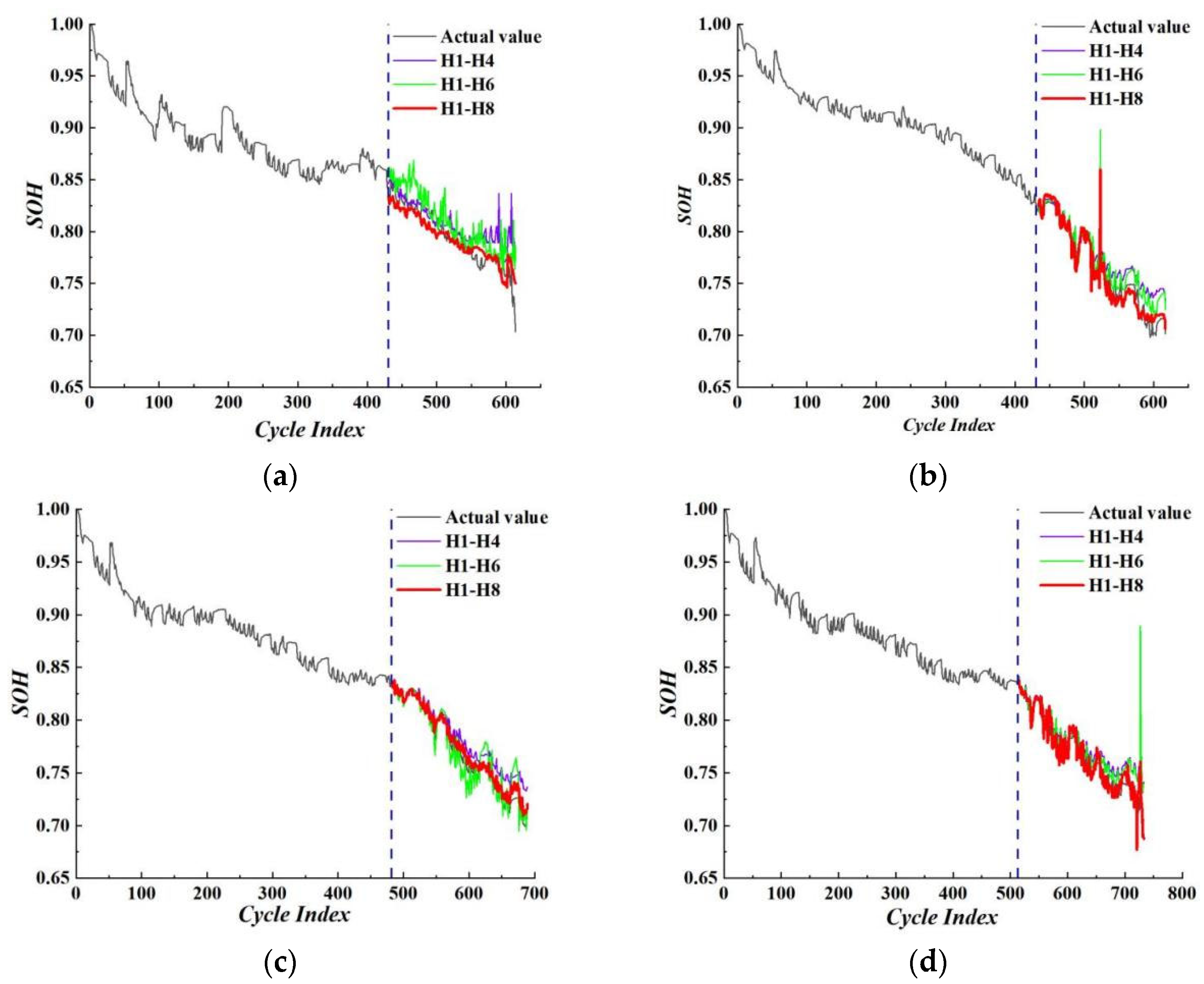
The size of the training set has a significant influence on the accuracy of SOH estimation. When the sample size is insufficient, the model may struggle to fully learn the nonlinear characteristics of the data, resulting in underfitting. Conversely, an excessively large training set may lead to overfitting, thereby reducing the model’s generalization ability. To examine this effect, this study selected four battery samples—B0005, B0006, B0007, and B0018—from the NASA dataset and constructed training sets using the first 50%, 60%, and 70% of each sample’s cycle data. A systematic analysis was conducted to evaluate how variations in training set size affect the prediction performance of the AO-AVOA-BP model. The prediction results and corresponding error metrics under different training proportions are presented in Figure 12 and

Table 10. SOH estimation error evaluation index under different training sets of NASA battery dataset.

Battery Number	Training Sets	MAE	RMSE	MAPE
B0005	50%	0.0146	0.0175	1.9908%
	60%	0.0083	0.0111	1.1252%
	70%	0.0059	0.0065	0.8320%
B0006	50%	0.0101	0.0131	1.6248%
	60%	0.0063	0.0073	0.9981%
	70%	0.0048	0.0057	0.7811%
B0007	50%	0.0150	0.0181	1.9412%
	60%	0.0111	0.0127	1.4393%
	70%	0.0067	0.0071	0.8808%
B0018	50%	0.0128	0.0151	1.7024%
	60%	0.0088	0.0104	1.1802%
	70%	0.0062	0.0072	0.8383%

.

Table 10 presents the prediction error metrics (MAE, RMSE, and MAPE) of the AO-AVOA-BP model under different training set proportions (50%, 60%, and 70%) across four NASA battery datasets (B0005, B0006, B0007, and B0018). Overall, as the proportion of training data increases, the prediction errors for all batteries consistently decrease, indicating a gradual improvement in model accuracy. Specifically, when the training set size increases from 50% to 70%, the MAE for battery B0005 drops significantly from 0.0146 to 0.0059, while the MAPE decreases from 1.9908% to 0.8320%. For B0006, the MAE declines from 0.0101 to 0.0048, with MAPE reduced by more than 50%. Similar trends are observed for B0007 and B0018, both achieving their lowest error levels at the 70% training ratio. Compared with the 50% training set, the 70% training set reduces MAE, RMSE, and MAPE by approximately 55–65% on average, significantly enhancing the model’s ability to capture SOH nonlinear features and improve trend prediction accuracy. Even relative to the 60% training set, the 70% setting maintains a further error reduction of about 20–30%. This improvement is attributed to the richer gradient information accumulated during training with the 70% dataset, which strengthens the model’s robustness in learning both early-stage and later-stage degradation trends, resulting in lower generalization errors on the test set. Therefore, this study adopts 70% of the cycle data as the training set, striking a balance between maximizing data utilization and avoiding the risk of overfitting due to excessive sample size. The results demonstrate that this proportion yields the optimal trade-off between stability and predictive accuracy, making it the most effective training configuration for SOH estimation using the AO-AVOA-BP model.

5.4. Impact of Different Health Factor Combinations on SOH Estimation Results

In the study of lithium-ion battery health state assessment, the appropriate selection of feature parameters plays a critical role in determining the predictive accuracy of the model. To evaluate the effectiveness of the proposed health factor combination in this work, four batteries—CS2-35, CS2-36, CS2-37, and CS2-38—from the CALCE dataset were selected as case studies. For consistency, the first 70% of each battery’s cycle data was used to construct the training set, with the remaining data serving as the test set. Under this experimental setup, the influence of different health factor combinations on the performance of the AO-AVOA-BP neural network model in the SOH estimation task was analyzed. The SOH prediction results for each battery are illustrated in Figure 13, while the corresponding error evaluation metrics are summarized in

Table 11. Evaluation index of SOH estimation error under different health factors in CALCE battery dataset.

Battery Number	Health Indicator	MAE	RMSE	MAPE
CS2-35	H1–H4	0.0141	0.0203	1.8276%
	H1–H6	0.0122	0.0156	1.2336%
	H1–H8	0.0087	0.0115	1.0950%
CS2-36	H1–H4	0.0130	0.0171	1.7737%
	H1–H6	0.0102	0.0155	1.3818%
	H1–H8	0.0072	0.0106	0.9303%
CS2-37	H1–H4	0.0116	0.0153	1.5627%
	H1–H6	0.0089	0.0122	1.1795%
	H1–H8	0.0051	0.0065	0.6748%
CS2-38	H1–H4	0.0122	0.0169	1.6376%
	H1–H6	0.0099	0.0160	1.3349%
	H1–H8	0.0075	0.0097	0.9837%

.

As shown in Figure 13, when the H1–H8 combination is used as input features, the predicted SOH curves closely align with the actual values, demonstrating high overall fitting accuracy. Moreover, the predicted trends exhibit the smallest fluctuations across all cycling stages, resulting in smoother and more stable estimations. This indicates that the selected feature combination not only effectively captures the degradation characteristics of battery performance but also significantly enhances the model’s sensitivity to SOH variations and its overall prediction stability.

Further analysis based on the data in Table 11 reveals that using the H1–H8 combination as input features yields significantly better SOH estimation performance across all battery samples compared to the H1–H4 and H1–H6 combinations. Specifically:

(1)

Substantial Reduction in Error Metrics: Taking the CS2-35 battery as an example, the H1–H8 combination results in MAE, RMSE, and MAPE of 0.0087, 0.0115, and 1.0950%, respectively. These values represent reductions of 38.3%, 43.3%, and 40.1% compared to the H1–H4 combination, and reductions of 28.7%, 26.3%, and 11.2% compared to the H1–H6 combination. A similar trend is observed for the CS2-36, CS2-37, and CS2-38 batteries. Notably, CS2-37 achieves a MAPE of only 0.6748% under the H1–H8 combination, the lowest among all feature groups.

(2)

Prominent Multi-Metric Superiority: The H1–H8 combination consistently achieves the best performance across all three error metrics (MAE, RMSE, and MAPE), indicating not only an improvement in overall predictive accuracy but also a reduction in local extreme errors. This reflects strong robustness and consistency in the model’s predictions.

(3)

Stable Performance Across Different Samples: Whether for CS2-35, CS2-36, CS2-37, or CS2-38, the H1–H8 combination consistently exhibits lower and more convergent error values. This suggests that the combination offers better generalization capability in SOH estimation across different batteries and cycling stages.

In summary, the H1–H8 health factor combination provides a more comprehensive and accurate representation of battery health state variations, thereby significantly enhancing the AO-AVOA-BP neural network model’s fitting accuracy and predictive stability. These results confirm the superiority and applicability of this feature set in the battery health state estimation task.

6. Conclusions

This study proposes a dual-mode intelligent optimization strategy that integrates the Arithmetic Optimization Algorithm (AO) and the African Vulture Optimization Algorithm (AVOA), and constructs the AO–AVOA–BP neural network model for high-precision State of Health (SOH) prediction of lithium-ion batteries. The research focuses on three main aspects: feature construction, parameter optimization, and performance validation, and leads to the following conclusions:

(1)

The integration of the AO and AVOA optimization mechanisms significantly enhances the global search capability and local convergence performance of the BP neural network. On the NASA and CALCE datasets, compared with the baseline BP model, the AO-AVOA-BP achieves reductions in MAE, RMSE, and MAPE by 72.9–85.7%, 69.6–85.2%, and 72.6–85.8%, respectively. These results are markedly superior to those of the PSO-BP, AO-BP, and AVOA-BP models, thereby providing strong evidence of the synergistic advantages of the dual-mode optimization mechanism in terms of both predictive accuracy and stability.

(2)

Eight health indicators are constructed based on charging-phase voltage, current, and temperature information. Feature selection is conducted using grey relational analysis, which substantially improves the physical relevance and interpretability of the model inputs.

(3)

The model consistently maintains stable prediction performance under varying training data proportions, battery samples, and degradation trajectories. It exhibits excellent generalization ability and engineering adaptability, and outperforms certain deep learning models in terms of computational complexity, making it suitable for deployment in embedded Battery Management Systems (BMS).

In summary, this study not only provides an effective modeling approach for improving the accuracy and robustness of battery SOH prediction, but also highlights the significant advantages of the AO–AVOA–BP model in predictive performance and stability through quantitative comparisons with multiple benchmark models. These findings expand the research boundaries of optimization algorithms in intelligent battery health modeling and demonstrate considerable theoretical significance as well as practical value.

In addition, the AO–AVOA–BP model still presents certain limitations. On the one hand, its relatively complex structure leads to high computational cost, posing challenges for deployment on resource-constrained embedded platforms. On the other hand, the model’s performance is to some extent dependent on hyperparameter configurations, which may restrict its generalization capability under varying operating conditions.

To enhance the engineering applicability of this research, future studies may proceed in the following three directions:

(1)

exploring model lightweighting techniques such as pruning and quantization to reduce computational and storage overhead, thereby improving the feasibility and real-time performance of deployment in practical battery management systems (BMS);

(2)

incorporating adaptive or parameter-free optimization mechanisms to lessen reliance on hyperparameter tuning and enhance model robustness across diverse scenarios;

(3)

conducting large-scale validations across different operating conditions, platforms, and battery chemistries to strengthen the model’s transferability and engineering applicability in both automotive and energy storage systems.

Such efforts would not only facilitate the translation of intelligent optimization algorithms into engineering practice but also provide strong support for the development of next-generation battery health management technologies.

References

1. Zhang, D.; Zhao, W.; Wang, L.; Chang, X.; Li, X.; Wu, P. Evaluation of the state of health of lithium-ion battery based on the temporal convolution network. Front. Energy Res. 2022, 10, 929235. [Google Scholar] [CrossRef]
2. Szürke, S.K.; Sütheö, G.; Őri, P.; Lakatos, I. Self-Diagnostic Opportunities for Battery Systems in Electric and Hybrid Vehicles. Machines 2024, 12, 324. [Google Scholar] [CrossRef]
3. Suanpang, P.; Jamjuntr, P. Optimal Electric Vehicle Battery Management Using Q-learning for Sustainability. Sustainability 2024, 16, 7180. [Google Scholar] [CrossRef]
4. Chen, X.; Chen, Z.; Wang, X.; Deng, Y. The integration of the convolutional neural network and fourier neural network methods for the battery pack capacity prediction. J. Energy Storage 2025, 125, 116907. [Google Scholar] [CrossRef]
5. Chen, X.; Wang, X.; Deng, Y. Federated learning-based prediction of electric vehicle battery pack capacity using time-domain and frequency-domain feature extraction. Energy 2025, 319, 135002. [Google Scholar] [CrossRef]
6. Zhang, F.; Xing, Z.X.; Wu, M.H. State of health estimation for Li-ion battery using characteristic voltage intervals and genetic algorithm optimized back propagation neural network. J. Energy Storage 2023, 57, 106277. [Google Scholar]
7. Zhao, K.; Liu, Y.; Zhou, Y.; Ming, W.; Wu, J. A Hierarchical and Self-Evolving Digital Twin (HSE-DT) method for multi-faceted battery situation awareness realisation. Machines 2025, 13, 175. [Google Scholar] [CrossRef]
8. Zuo, H.Y.; Liang, J.W.; Zhang, B.; Wei, K.X.; Zhu, H.; Tan, J.Q. Intelligent estimation on state of health of lithium-ion power batteries based on failure feature extraction. Energy 2023, 282, 128794. [Google Scholar] [CrossRef]
9. Demirci, O.; Taskin, S.; Schaltz, E.; Demirci, B.A. Review of battery state estimation methods for electric vehicles-Part II: SOH estimation. J. Energy Storage 2024, 96, 112703. [Google Scholar] [CrossRef]
10. Roman, D.; Saxena, S.; Robu, V.; Pecht, M.; Flynn, D. Machine learning pipeline for battery state-of-health estimation. Nat. Mach. Intell. 2021, 3, 447–456. [Google Scholar] [CrossRef]
11. Nuroldayeva, G.; Serik, Y.; Adair, D.; Uzakbaiuly, B.; Bakenov, Z. State of Health Estimation Methods for Lithium-Ion Batteries. Int. J. Energy Res. 2023, 2023, 4297545. [Google Scholar] [CrossRef]
12. Bian, X.L.; Wei, Z.B.; Li, W.H.; Pou, J.; Sauer, D.U.; Liu, L.C. State-of-health estimation of lithium-ion batteries by fusing an open circuit voltage model and incremental capacity analysis. IEEE Trans Power Electron 2022, 37, 2226–2236. [Google Scholar] [CrossRef]
13. Hosseininasab, S.; Lin, C.; Pischinger, S.; Stapelbroek, M.; Vagnoni, G. State-of-health estimation of lithium-ion batteries for electrified vehicles using a reduced-order electrochemical model. J. Energy Storage 2022, 52, 104684. [Google Scholar] [CrossRef]
14. Chen, G. Residual useful life prediction of lithium-ion battery based on accuracy SoH estimation. Sci. Rep. 2025, 15, 6010. [Google Scholar] [CrossRef] [PubMed]
15. Yang, G.; Wang, X.; Li, R.; Zhang, X. State of health estimation for lithium-ion batteries based on transferable long short-term memory optimized using harris hawk algorithm. Sustainability 2024, 16, 6316. [Google Scholar] [CrossRef]
16. Qiang, H.; Zhang, W.; Ding, K. A prediction framework for state of health of lithium-ion batteries based on improved support vector regression. J. Electrochem. Soc. 2023, 170, 110517. [Google Scholar] [CrossRef]
17. Li, Y.; Qin, X.; Ma, F.; Wu, H.; Chai, M.; Zhang, F.; Jiang, F.; Lei, X. Fusion Technology-Based CNN-LSTM-ASAN for RUL Estimation of Lithium-Ion Batteries. Sustainability 2024, 16, 9223. [Google Scholar] [CrossRef]
18. Li, H.; Ding, R.; Xi, Y.; Zhang, S.; Zhang, X. An online fine-tuning method for modelling online SOH estimation under multi-stage constant current charging protocol. J. Energy Storage 2025, 128, 117233. [Google Scholar] [CrossRef]
19. Tong, L.; Li, Y.; Chen, Y.; Kuang, R.; Xu, Y.; Zhang, H.; Peng, B.; Yang, F.; Zhang, J.; Gong, M. State of health estimation for lithium-ion batteries based on fusion health features and adaboost-GWO-BP model. J. Electrochem. Soc. 2024, 171, 110528. [Google Scholar] [CrossRef]
20. Gong, Q.R.; Wang, P.; Cheng, Z. An encoder-decoder model based on deep learning for state of health estimation of lithium-ion battery. J. Energy Storage 2022, 46, 103804. [Google Scholar] [CrossRef]
21. Lei, L.; Haihong, H. A fast method for estimating remaining useful life of energy storage battery based on bidirectional synthetic square wave detection and ASO-BP. J. Energy Storage 2025, 112, 115454. [Google Scholar] [CrossRef]
22. Ma, Y.; Yao, M.H.; Liu, H.C.; Tang, Z.G. State of Health estimation and Remaining Useful Life prediction for lithium-ion batteries by Improved Particle Swarm Optimization-Back Propagation Neural Network. J. Energy Storage 2022, 52, 104750. [Google Scholar] [CrossRef]
23. Farong, K.; Dongming, Z.; Tianxiang, Y.; Xi, L. State of health estimation of lithium-ion batteries based on maximal information coefficient feature optimization and GJO-BP neural network. Ionics 2025, 31, 3311–3322. [Google Scholar] [CrossRef]
24. Chandran, V.; Mohapatra, P. A boosted African vultures optimization algorithm combined with logarithmic weight inspired novel dynamic chaotic opposite learning strategy. Expert Syst. Appl. 2025, 271, 126532. [Google Scholar] [CrossRef]
25. Liu, R.J.; Wang, T.L.; Zhou, J.; Hao, X.X.; Xu, Y.; Qiu, J.Z. Improved African vulture optimization algorithm based on quasi-oppositional differential evolution operator. IEEE Access 2022, 10, 95197–95218. [Google Scholar] [CrossRef]
26. Alizadeh, A.; Gharehchopogh, F.S.; Masdari, M.; Jafarian, A. An improved hybrid salp swarm optimization and African vulture optimization algorithm for global optimization problems and its applications in stock market prediction. Soft Comput. 2024, 28, 5225–5261. [Google Scholar] [CrossRef]
27. Mostafa, R.R.; Hashim, F.A.; El-Attar, N.E.; Khedr, A.M. Empowering African vultures optimizer using Archimedes optimization algorithm for maximum efficiency for global optimization and feature selection. Evol. Syst. 2024, 15, 1701–1731. [Google Scholar] [CrossRef]
28. Duan, W.; Song, S.; Xiao, F.; Chen, Y.; Peng, S.; Song, C. Battery SOH estimation and RUL prediction framework based on variable forgetting factor online sequential extreme learning machine and particle filter. J. Energy Storage 2023, 65, 107322. [Google Scholar] [CrossRef]
29. Abualigah, L.; Yousri, D.; Elaziz, M.A.; Ewees, A.A.; Al-Qaness, M.A.; Gandomi, A.H. Aquila optimizer: A novel meta-heuristic optimization algorithm. Comput. Ind. Eng. 2021, 157, 107250. [Google Scholar] [CrossRef]
30. Abdollahzadeh, B.; Gharehchopogh, F.S.; Mirjalili, S. African vultures optimization algorithm: A new nature-inspired metaheuristic algorithm for global optimization problems. Comput. Ind. Eng. 2021, 158, 107408. [Google Scholar] [CrossRef]
31. Zhang, M.; Yang, D.; Du, J.; Sun, H.; Li, L.; Wang, L.; Wang, K. A review of SOH prediction of Li-ion batteries based on data-driven algorithms. Energies 2023, 16, 3167. [Google Scholar] [CrossRef]
32. Mao, Q.H.; Wang, Y.G.; Niu, X.H. Improved mayfly optimization algorithm based on anti-attraction velocity update mechanism. J. Beijing Univ. Aeronaut. Astronaut. 2024, 50, 1770–1783. [Google Scholar]
33. Li, H.L.; Liu, X.C.; Gao, Q.; He, G.G.; Song, H. Lithium-ion battery state of health estimation based on TCT-PSA modeling. Electron. Meas. Technol. 2024, 47, 122–131. [Google Scholar]
34. Meng, H.X.; Geng, M.Y.; Han, T. Long short-term memory network with Bayesian optimization for health prognostics of lithium-ion batteries based on partial incremental capacity analysis. Reliab. Eng. Syst. Saf. 2023, 236, 109288. [Google Scholar] [CrossRef]
35. Zhang, H.; Gao, J.; Kang, L.; Zhang, Y.; Wang, L.; Wang, K. State of health estimation of lithium-ion batteries based on modified flower pollination algorithm-temporal convolutional network. Energy 2023, 283, 128742. [Google Scholar] [CrossRef]
36. Jia, Z.; Li, Z.; Zhao, K.; Wang, K.; Wang, S.; Liu, Z. CNN-DBLSTM: A long-term remaining life prediction framework for lithium-ion battery with small number of samples. J. Energy Storage 2024, 97, 112947. [Google Scholar] [CrossRef]
37. Wu, S.; Li, D.; Xing, W.; Liu, Y. Quantitative prediction model for lithium-ion battery life uncertainty based on DAE-CNN-BiGRU quantile regression. J. Energy Storage 2025, 123, 116771. [Google Scholar] [CrossRef]
38. Zhou, K.; Zhang, Z. Remaining useful life prediction of lithium-ion batteries based on data denoising and improved transformer. J. Energy Storage 2024, 100, 113749. [Google Scholar] [CrossRef]
Figure 1. SOH variation curve of lithium-ion battery.
Machines 13 00799 g001
Figure 2. Charging curves with different cycle numbers. (a) Charging cycle current variation curve. (b) Charging cycle voltage variation curve.
Machines 13 00799 g002
Figure 3. Curves of changing capacity and time at different charging stages. (a) Variation in the CC charging capacity and time. (b) Variation in the CV charging capacity and time.
Machines 13 00799 g003
Figure 4. Temperature change curves under different cycles.
Machines 13 00799 g004
Figure 5. Change curves of temperature rise and mean temperature of the battery.
Machines 13 00799 g005
Figure 6. Improved AO-AVOA dual-mode intelligent optimization algorithm flow chart.
Machines 13 00799 g006
Figure 7. Flowchart of the AO-AVOA-BP model.
Machines 13 00799 g007
Figure 8. Overall Flow Chart.
Machines 13 00799 g008
Figure 9. Convergence curves under different test functions. (a) Test function F 1 x . (b) Test function F 2 x . (c) Test function F 3 x . (d) Test function F 4 x . (e) Test function F 5 x . (f) Test function F 6 x .
Machines 13 00799 g009
Figure 10. SOH prediction results and errors of different models of NASA battery. (a) B0005 Predictive Curve. (b) B0005 Deviation Curve. (c) B0006 Predictive Curve. (d) B0006 Deviation Curve. (e) B0007 Predictive Curve. (f) B0007 Deviation Curve. (g) B0018 Predictive Curve. (h) B0018 Deviation Curve.
Machines 13 00799 g010
Figure 11. SOH prediction results and errors of different models of CALCE battery. (a) CS2-35 Predictive Curve. (b) CS2-35 Deviation Curve. (c) CS2-36 Predictive Curve. (d) CS2-36 Deviation Curve. (e) CS2-37 Predictive Curve. (f) CS2-37 Deviation Curve. (g) CS2-38 Predictive Curve. (h) CS2-38 Deviation Curve.
Machines 13 00799 g011
Figure 12. The evaluation index comparison chart of different training sets of NASA battery dataset. (a) MAE. (b) RMSE. (c) MAPE.
Machines 13 00799 g012
Figure 13. SOH prediction results under different health factors in CALCE battery dataset. (a) CS2-35. (b) CS2-36. (c) CS2-37. (d) CS2-38.
Machines 13 00799 g013