Modeling and Validation of a Spring-Coupled Two-Pendulum System Under Large Free Nonlinear Oscillations

Abstract

Studying nonlinear oscillations in mechanical systems is fundamental to understanding complex dynamic behavior in engineering applications. While classical analytical methods remain valuable for systems with limited complexity, they become increasingly inadequate when nonlinearities are strong and geometrically induced, as in the case of large-amplitude oscillations. This paper presents a combined numerical and experimental investigation of a mechanical system composed of two coupled pendulums, exhibiting significant nonlinear behavior due to elastic deformation throughout their motion. A mathematical model of the system was developed using the MatLab/Simulink ver.6.1 environment, considering gravitational, inertial, and nonlinear elastic restoring forces. One of the major challenges in accurately modeling such systems is accurately representing damping, particularly in the absence of dedicated dampers. In this work, damping coefficients were experimentally identified through decrement measurements and incorporated into the simulation model to improve predictive accuracy. The simulation outputs, including angular displacements, velocities, accelerations, and phase trajectories over time, were validated against experimental results obtained via high-precision inertial sensors. The comparison shows a strong correlation between numerical and experimental data, with minimal relative errors in amplitude and frequency. This research represents the first stage of a broader study aimed at analyzing forced and parametrically excited oscillations. Beyond validating the model, the study contributes to the design of a robust experimental framework suitable for further exploration of nonlinear dynamics. The findings have practical implications for the development and control of mechanical systems subject to dynamic loads, with potential applications in automation, vibration analysis, and system diagnostics.

1. Introduction

The pendulum, in its simplicity, has long held a distinguished place in the history of science and engineering. From the earliest contemplations of periodic motion to the development of high-precision timekeeping instruments, the pendulum has long served as both a physical system and a conceptual model. The timeless intrigue of its dynamics stems not only from its observable periodic behavior but also from its ability to display strongly nonlinear and potentially chaotic behavior under specific conditions. This dual character, characterized by simplicity in structure and complexity in behavior, has made the pendulum a paradigmatic system in the study of classical and nonlinear mechanics.

Historically, the study of pendulums gained prominence during the Renaissance. Leonardo da Vinci made early observations and sketches of pendular motion, laying the groundwork for later systematic studies of this phenomenon. Galileo Galilei, often credited with pioneering the quantitative analysis of pendulum motion, discovered the isochronism of small angular oscillations, noting that the period of a pendulum remains constant, within certain limits, regardless of amplitude [1]. This insight led to fundamental advances in physics and mechanics, paving the way for a new era of experimental investigation and theoretical modeling.

The 17th century witnessed a major technological breakthrough when Christiaan Huygens applied Galileo’s principles to develop the first pendulum clock in 1656. Huygens’ invention transformed timekeeping and catalyzed the scientific revolution by establishing a reliable standard for precise timekeeping [2]. Nearly two centuries later, the pendulum once again demonstrated its scientific power when Jean-Bernard Léon Foucault used a long and heavy pendulum to confirm Earth’s rotation experimentally. Suspended from the dome of the Panthéon in Paris, Foucault’s pendulum offered a compelling visual demonstration of Earth’s rotation, achieved without reliance on an astronomical instrument [3].

These historical milestones elevated the pendulum from mere curiosity to a cornerstone of experimental physics and applied mechanics. Its mathematical description, derived from Newtonian mechanics, served as one of the earliest examples of differential equation modeling in physical systems. While linear approximations suffice for small angular displacements, the pendulum’s full motion is governed by nonlinear equations that pose considerable analytical challenges.

To address the inherent nonlinearities, various analytical methods have been proposed over the years. Techniques such as the method of multiple scales, harmonic balance, perturbation theory, and elliptic integral approaches have been extensively used to approximate the behavior of pendulum systems undergoing large angular oscillations [4,5,6,7]. These methods have proven particularly effective in studying complex dynamics problems in classical mechanics, vibration analysis, and in areas such as control theory and chaos analysis.

In addition, the scope of research on pendulums has expanded beyond single-degree-of-freedom systems to include multiple and complexly connected configurations exhibiting increasingly rich dynamic behavior. The double pendulum, consisting of two interconnected pendular arms, represents a canonical example of a system with multiple degrees of freedom and high sensitivity to initial conditions. Its dynamics are highly nonlinear and can exhibit chaotic regimes even at moderate energy. This complexity makes it an ideal model for exploring the transition from periodic to chaotic motion, bifurcations, and energy exchange between system components [8].

As the theoretical foundation of pendulum dynamics matured, researchers began to complement analytical approaches with numerical simulations. With the rise of modern computing and mathematical software environments, such as MatLab and Simulink, it has become possible to model and simulate pendulum systems with high fidelity, including nonlinear stiffness, damping, and coupling effects. These tools enable the simulation of coupled nonlinear differential equations that describe the motion of the pendulum under various initial conditions and different external influences.

A major advantage of numerical methods is their flexibility in incorporating experimentally determined parameters. For instance, in real mechanical systems, damping is rarely well defined and may stem from multiple sources, including air resistance, internal material friction, and mechanical joint losses. Although analytical models typically assume idealized or linear damping, experimental methods yield more realistic damping estimates based on physical behavior. Damping coefficients can be estimated from free decay tests using logarithmic decrement methods, allowing for improved alignment between simulation and observation [9].

The recent literature demonstrates the diversity of methodologies applied to pendulum systems. In [10], successive maxima maps are used to identify complex dynamic regimes in magnetic pendulums. Study [11] applies multiscale perturbation methods to determine nonlinear natural frequencies and explores the drift of modal behavior as amplitude increases. The methodology in [12] highlights the use of rational torque approximations and numerical analysis in robotic and manipulator applications. These works underscore the adaptability of pendulum systems as experimental platforms and test beds for advanced theoretical frameworks.

The research in [13] utilizes the complex behavior of the double pendulum to highlight some well-known techniques that can be employed to understand the dynamics and solutions better. Analytical and numerical methods, implemented using the MatLab package, are successfully contrasted to illustrate their usefulness and limitations.

An important contribution in [14] demonstrates that the double pendulum system is a general and typical model for studying nonlinear dynamics due to the diverse and complex dynamic phenomena. The paper examines the impact of various parameters on the system, including the pendulum length and initial release angle.

A particularly illustrative set of investigations examines the behavior of double pendulums with varying structural and dynamic parameters. In [15], the authors conduct a theoretical and numerical analysis of a double pendulum system with variable mass. Four scenarios are considered: a classical configuration with fixed masses, a system with a variable upper mass, one with a variable lower mass, and a configuration where both masses vary. For each case, the authors develop and solve differential equations using the fourth-order Runge–Kutta method. The simulation results reveal how mass variability affects system stability and oscillatory behavior, providing insight into nonlinear mass-dependent dynamics.

In [16], the study focuses on the onset of chaotic motion in a double pendulum system due to variations in initial conditions. Using the Lagrangian and Hamiltonian formalisms, the authors derive the system’s equations of motion and apply numerical simulations to investigate key indicators of chaos, including Poincaré sections, Lyapunov exponents, and trajectory divergence. The work highlights the system’s extreme sensitivity to initial inputs and the resulting complexity in motion prediction.

A different approach is explored in [17], where the authors analyze a two-degree-of-freedom pendulum system equipped with permanent magnets at the free ends. The study presents a new experimentally validated model for magnetic force interactions, combining time-domain measurements with bifurcation diagrams, phase portraits, and Poincaré maps to analyze the system’s nonlinear behavior. The findings demonstrate the strong influence of magnetic coupling on the system’s dynamic evolution.

The synchronization of coupled pendulums is examined in [18,19]. These studies explore phase shift behavior between disconnected pendulums and employ both analytical and numerical techniques to evaluate synchronization under various excitation conditions. Harmonic linearization methods are used to derive phase relations, while simulations confirm the analytical predictions and illustrate the conditions under which synchronization is stable or disrupted.

Large amplitude oscillations of a pendulum attached to a rotating structure are studied in [20]. By employing a combination of Maclaurin series expansion and orthogonal Chebyshev polynomials, the authors reduce the governing nonlinear equations to a cubic-quintic Duffing equation. This formulation enables the use of an iterative analytical approach to solve the resulting timing problem and to capture the effects of complex rotational coupling.

In [21], the authors investigate nonlinear spatial oscillations of a point mass suspended on a weightless elastic medium. They assume a condition where the vertical oscillation frequency equals twice the swing frequency, leading to instability in vertical motion and energy transfer to horizontal swinging. The work also explores forced oscillations in a spring pendulum subject to friction, applying the averaging method to construct an asymptotic solution. The study establishes analogies with gas bubble deformation oscillations, enhancing interdisciplinary insight into nonlinear dynamics.

Study [22] presents a detailed analysis of a double pendulum rotating at a constant speed about a vertical axis through its upper hinge. The authors identify transitions from chaotic to quasi-periodic motion and back as the rotation speed increases. Internal resonance effects are shown to produce new equilibrium states and promote the emergence of complex oscillatory modes. Analytical and numerical methods are employed to characterize the system’s bifurcation structure and stability zones.

Control strategies using periodic forcing are the focus of [23]. Here, the authors demonstrate that periodic open-loop excitation can stabilize the inverted position of a single-degree-of-freedom pendulum. The average potential method is used to assess equilibrium stability, with implications for controlling multi-link pendulums and oscillating trolleys on inclined surfaces. Bifurcation behavior and control performance are analyzed under various forcing conditions.

In [24], the authors study orbital stability in periodic pendulum motion, assuming synchronized oscillations with matched amplitudes and directions. For systems with low stiffness or small amplitude, analytical methods yield stability conditions. When parameters become strongly nonlinear, numerical simulations are used to map out the dynamic response, providing insight into transitions from stable to unstable motion.

This analysis is extended in [25], where the effects of varying stiffness and amplitude are explored through a series of simulations. The combined findings emphasize the importance of integrating analytical and computational techniques to accurately predict stability boundaries and response characteristics in coupled pendulum systems.

Finally, work [26] investigates quasilinear conservative systems with two degrees of freedom using differential equations derived from classical mechanics. By employing the Bogolyubov–Mitropolsky asymptotic method, approximate analytical solutions are developed for representative mechanical configurations. The authors also analyze resonance and energy transfer phenomena in a beam-pendulum system, validating their results through experimental comparison. These studies underscore the critical role of asymptotic methods in analyzing nonlinear dynamic interactions within mechanical structures.

The review of the key contributions presented above further reflects a growing trend toward hybrid analytical–computational models, which enable more accurate and efficient representation of nonlinear phenomena in complex mechanical systems.

Although pendulum-based systems have been widely studied, novel configurations—such as the one analyzed in this study, involving two pendulums coupled by elastic springs and subject to internal damping and large angular displacements—require specialized numerical methods for accurate analysis. The pronounced nonlinearity of the governing differential equations renders closed-form analytical solutions impossible. Consequently, the development of a dedicated computational strategy is crucial for accurately integrating the system’s equations of motion.

Prior to the emergence of modern computational tools, particularly in the late 19th and early 20th centuries, the study of nonlinear differential equations largely relied on linearization methods. These classical approaches, developed by pioneers such as Poincaré, Van der Pol, Bogolyubov, Mitropolsky, and Chebyshev, among others [17,18,19,20,26], are primarily suitable for weakly nonlinear systems where a small parameter can be identified. In contrast, the system analyzed in this study exhibits strong nonlinearities that preclude the application of such analytical techniques. Additionally, frequency-domain analysis proves inadequate due to the complexity and coupled nature of dynamics. Therefore, the investigation is conducted using a numerical approach implemented in the MatLab environment, in line with the methodologies reported in [13,15].

The present study is positioned in this context. It is an extended version of the work presented at the SIELA 2024 conference [27]. The paper focuses on a two-degree-of-freedom mechanical system consisting of two coupled pendulums. The main objective is to investigate the nonlinear oscillatory behavior of the system using a hybrid methodology that integrates numerical simulation with experimental validation. A mathematical model based on Newtonian mechanics is formulated that captures the most important forces acting on each pendulum, including gravitational, inertial, and coupling force effects. The equations of motion are derived and numerically integrated using MatLab and Simulink toolbox.

A critical aspect of this work involves estimating and including damping. Since the system lacks explicit damping elements, such as hydraulic vibration dampers, an experimental procedure was employed to calculate the logarithmic decrement based on the measured free oscillation amplitudes of the two pendulums at various time scales. The damping coefficient thus determined was used to obtain the finite differential equations of motion of the two pendulums. This approach yielded highly accurate numerical results for angular displacements, velocities, accelerations, and phase portraits, which closely matched the experimental data obtained using high-resolution inertial sensors.

In the studied system, energy loss is attributed to internal friction within the springs, as well as to dry friction in the bearings and joints. To address this highly complex problem, elastic-viscous models such as those of Voigt and Rayleigh have been successfully applied in the context of linear systems. These models allow for the decomposition of the system’s differential equations and their straightforward integration. However, in the case of nonlinear systems, this approach becomes impractical. The book by Nasif A. D. et al. [28] discusses various methods that can be employed for complex damping devices. The system under investigation, however, is characterized by strong geometric nonlinearity, and the only viable method for obtaining a dynamic model that adequately accounts for damping effects is a combined theoretical and experimental approach. This involves measuring the initial and final amplitudes of all kinematic parameters over an extended period, e.g., 120 s, using accelerometric sensors. The resulting damping coefficients are then incorporated into the system of differential equations, and after integration, the numerical results closely match the experimentally measured data. This constitutes the most significant scientific and applied contribution of the present study.

The experimental setup was specifically designed to capture the detailed motion characteristics of the pendulum arms. Sensor-based measurements enabled the reconstruction of time histories and dynamic responses, offering a robust foundation for comparison with the results of numerical simulations. This approach enables the rigorous validation of the model and the identification of potential discrepancies that may arise from various non-ideal connections, dry friction in the bearings, or measurement noise.

This study represents the initial phase of a broader research initiative. While the current focus is on free oscillations, the validated model will serve as a basis for future studies of forced oscillations. Such further studies will allow for the analysis of resonance phenomena, force responses, and strategies for avoiding beating, transient regimes, and for different excitation profiles.

The two-pendulum system, particularly in its nonlinear and spring-coupled form, has significant applications in the study of complex dynamic behavior. It serves as a fundamental model in nonlinear dynamics, providing insights into sensitivity to initial conditions, bifurcations, and energy transfer in multi-body systems. In precision instrumentation, such systems are relevant for understanding synchronization effects in coupled oscillators, with implications for timekeeping devices and resonant sensors. Moreover, due to its analytical richness and visual demonstrability, the two-pendulum system is widely used in educational contexts to teach advanced concepts in classical mechanics, such as Lagrangian dynamics, phase space analysis, and numerical integration of nonlinear differential equations.

This paper develops the classical ideas of nonlinear dynamics based on a mechanical system of two coupled pendulums, providing a modern, integrated numerical and experimental approach. By combining theoretical modeling with experimental data, the study achieves a high degree of model validation, laying the foundation for future work in areas such as design, control, vibration isolation, and adaptive monitoring algorithms in complex mechatronic applications.

The findings presented here highlight the continued relevance of pendulum systems as versatile and rich platforms for studying nonlinear dynamics. They are a classic example and a contemporary engineering challenge. Pendulums continue to provide valuable insights into the behavior of complex systems, including coupling, damping effects, and control strategies that span both theoretical and applied areas.

2. Dynamical Model of the Pendulum Spring System

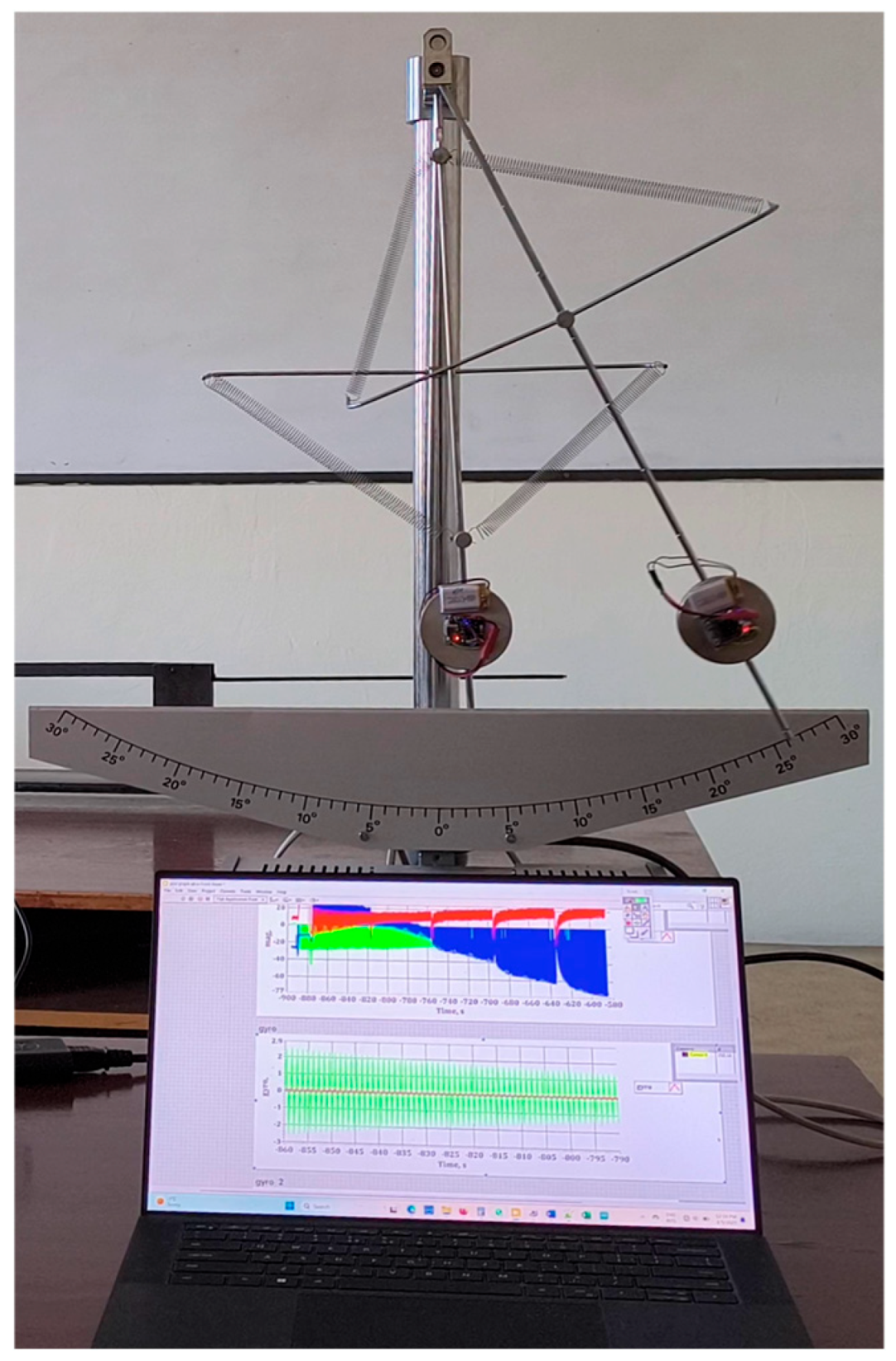
The general appearance of the device for studying the large angular oscillations of a mechanical system, which consists of two connected pendulums, is shown in Figure 1.

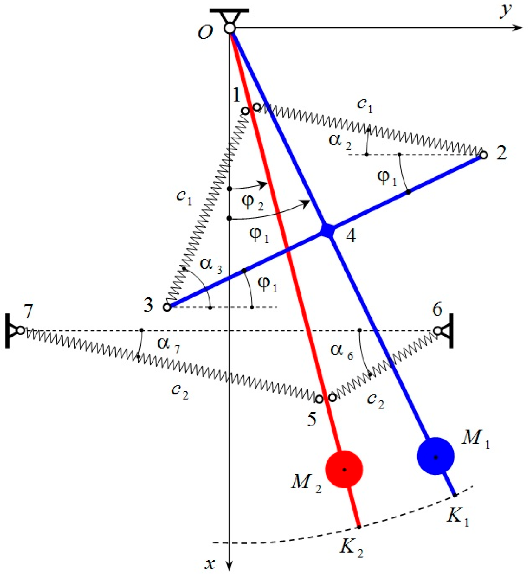
The dynamical model of this device is shown in Figure 2. It consists of two pendulums: a front pendulum $M_{1 }$ and a rear pendulum $M_2$, which rotate about a common horizontal axis. The main rods of the pendulum are made of steel with a diameter $d =5.1 \mathrm{m}\mathrm{m}$ and lengths ${OK}_1={OK}_2=510 \mathrm{m}\mathrm{m}$.

At a certain fixed distance along the length of these rods, ${OM}_1 = 417 \mathrm{m}\mathrm{m} \mathrm{a}\mathrm{n}\mathrm{d} O{M}_2 = 384 \mathrm{m}\mathrm{m}$, two cylindrical bodies with a diameter $\mathrm{of} D = 60.5 \mathrm{m}\mathrm{m}$ and a thickness $\mathrm{of} h = 11.8 \mathrm{m}\mathrm{m}$ are placed. These bodies have a mass $\mathrm{o}\mathrm{f} m = 100 \mathrm{g}$. The front pendulum has a transverse rod with a diameter of $d = 3 \mathrm{m}\mathrm{m}$ and a length of $l_{23} = 300 \mathrm{m}\mathrm{m}$. The springs connecting points 1 and 2, as well as 1 and 3, have elasticity coefficients $c_1=6.173 \mathrm{N}/\mathrm{m}$. At rest and stable equilibrium, these springs are inclined at an angle $\alpha ={41.88}^{°}$ toward the horizon.

The spring connecting points 5 and 6, as well as points 5 and 7, has an elasticity coefficient $c_2 = 6.562 \mathrm{N}/\mathrm{m}$. At rest and stable equilibrium, these springs are inclined at an angle $\beta ={20.47}^0$ to the horizon.

The other geometric dimensions of the pendulum device are as follows:

$l_{01} = 52.5 \mathrm{m}\mathrm{m}$, $l_{04} = 187 \mathrm{m}\mathrm{m}$, $l_{24} = l_{34} = 150 \mathrm{m}\mathrm{m}$, $l_{08} = 266 \mathrm{m}\mathrm{m}$, $l_{58} = 56 \mathrm{m}\mathrm{m}$, $l_{05} = 322 \mathrm{m}\mathrm{m}$, $l_{14} = 134.5 \mathrm{m}\mathrm{m}$, $l_{68} = l_{78} = 150 \mathrm{m}\mathrm{m}$.

The two disks, combined with the rods, are modeled as physical pendulums. The positions of their mass centers $C_1$ and $C_2$, as well as the mass moments of inertia $J_1$ and $J_2$, have been determined. They are:${ OC}_1 = 327.4 \mathrm{m}\mathrm{m},$ ${OC}_2 = 326 \mathrm{m}\mathrm{m},$ $J_1 = 0.02592 \mathrm{k}\mathrm{g}·{\mathrm{m}}^2$ and $J_2 = 0.02188 \mathrm{k}\mathrm{g}·{\mathrm{m}}^2$.

The mechanical system has two degrees of freedom. The two angles ${\phi }_1$ and ${\phi }_2$ are accepted for generalized coordinates (Figure 2).

Differential equations that describe the large oscillations of the two pendulums, in compact form, have the form:

$$J_1 {\ddot{\phi }}_1+b_1 {\dot{\phi }}_1=-m_{1}g O{C}_1\mathit{sin}{\phi }_1+M_1\left({\phi }_1,{\phi }_2\right),$$

(1)

$$J_2 {\ddot{\phi }}_2+b_2 {\dot{\phi }}_2=-m_{2}g O{C}_{2 }\mathit{sin}{\phi }_2+M_2\left({\phi }_1,{\phi }_2\right).$$

(2)

where $g=9.81\mathrm{m}/{\mathrm{s}}^2$, $M_1\left({\phi }_1,{\phi }_2\right)$, and $M_2\left({\phi }_1,{\phi }_2\right)$ are the moments of the elastic forces from the springs, and $b_1$ and $b_2$ are damping coefficients that are determined experimentally using a methodology that is described at the end of this section.

The detailed records of these moments are:

$$M_1\left({\phi }_1,{\phi }_2\right)=F_{{12}_V} y_2-F_{{12}_H} x_2+F_{{13}_H} x_3+F_{{13}_V} y_3,$$

(3)

$$M_2\left({\phi }_1,{\phi }_2\right)=\left(F_{{12}_H}-F_{{13}_H}\right) x_1-\left(F_{{12}_V}+F_{{13}_V}\right) y_1+\left(F_{{56}_H}-F_{{57}_H}\right) x_5+\left(F_{{56}_V}+F_{{57}_V}\right) y_5,$$

(4)

where $x_1$, $y_1$, $x_2$, $y_2$, $x_3$, $y_3$, $x_5$, and $y_5$ are the coordinates of the moving points 1, 2, 3, and 5, and $F_{{ij}_H}$ и $F_{{ij}_V}$, $(i=1, 5; j=2, 3, 6, 7)$ are the horizontal and vertical components of the elastic forces $F_{ij}$ in the springs.

The formulas determine these components:

$$F_{{12}_H}=F_{12} \mathit{cos}{\alpha }_2, F_{{12}_V}=F_{12} \mathit{sin}{\alpha }_2,$$

(5)

$$F_{{13}_H}=F_{13} \mathit{cos}{\alpha }_3, F_{{13}_V}=F_{13} \mathit{sin}{\alpha }_3,$$

(6)

$$F_{{56}_H}=F_{56} \mathit{cos}{\alpha }_6, F_{{56}_V}=F_{56} \mathit{sin}{\alpha }_6,$$

(7)

$$F_{{57}_H}=F_{57} \mathit{cos}{\alpha }_7, F_{{57}_V}=F_{57} \mathit{sin}{\alpha }_7.$$

(8)

The sines and cosines of variable angles ${\alpha }_2$, ${\alpha }_3$, ${\alpha }_6$, and ${\alpha }_7$ are determined by the formulas:

$$\mathit{cos}{\alpha }_2={\displaystyle \frac{\left|y_1-y_2\right|}{L_{12}}}, \mathit{sin}{\alpha }_2={\displaystyle \frac{\left|x_1-x_2\right|}{L_{12}}},$$

(9)

$$\mathit{cos}{\alpha }_3={\displaystyle \frac{\left|y_1-y_3\right|}{L_{13}}}, \mathit{sin}{\alpha }_3={\displaystyle \frac{\left|x_1-x_3\right|}{L_{13}}},$$

(10)

$$\mathit{cos}{\alpha }_6={\displaystyle \frac{\left|y_5-Y_6\right|}{L_{56}}}, \mathit{sin}{\alpha }_6={\displaystyle \frac{\left|x_5-X_6\right|}{L_{56}}},$$

(11)

$$\mathit{cos}{\alpha }_7={\displaystyle \frac{\left|y_5-Y_7\right|}{L_{57}}}, \mathit{sin}{\alpha }_7={\displaystyle \frac{\left|x_5-X_7\right|}{L_{57}}}.$$

(12)

where the formulas obtain dynamic variable lengths of the springs:

$$L_{12}=\sqrt{{\left(x_1-x_2\right)}^2+{\left(y_1-y_2\right)}^2},$$

(13)

$$L_{13}=\sqrt{{\left(x_1-x_3\right)}^2+{\left(y_1-y_3\right)}^2},$$

(14)

$$L_{56}= \sqrt{{\left(x_5-X_6\right)}^2+{\left(y_5-Y_6\right)}^2},$$

(15)

$$L_{57}=\sqrt{{\left(x_5-X_7\right)}^2+{\left(y_5-Y_7\right)}^2}.$$

(16)

The formulas determine elastic forces:

$$F_{12}=c_1 L_{12},$$

(17)

$$F_{13}=c_1 L_{13},$$

(18)

$$F_{56}=c_2 L_{56},$$

(19)

$$F_{57}=c_2 L_{57}.$$

(20)

Finally, we will show the formulas through which the coordinates of movable points 1, 2, 3, and 5 are determined, namely:

$$x_1=l_{01} \mathit{cos}{\phi }_2, y_1=l_{01} \mathit{sin}{\phi }_2,$$

(21)

$$x_2=l_{04} \mathit{cos}{\phi }_1-l_{24} \mathit{sin}{\phi }_1, y_2=l_{04} \mathit{sin}{\phi }_1+l_{24} \mathit{cos}{\phi }_1,$$

(22)

$$x_3=l_{04} \mathit{cos}{\phi }_1+l_{34} \mathit{sin}{\phi }_1, y_3=l_{04} \mathit{sins}{\phi }_1-l_{34} \mathit{cos}{\phi }_1$$

(23)

$$x_5=l_{05} \mathit{cos}{\phi }_2, y_5=l_{05} \mathit{sin}{\phi }_2.$$

(24)

The coordinates of the fixed points are:

$$X_6=X_7=0.266 \mathrm{m}, Y_6=0.15 \mathrm{m}, Y_7=-0.15 \mathrm{m}.$$

(25)

The two damping coefficients from Equations (1) and (2) are determined using the formula:

$$b_n=2 {\displaystyle \frac{\mathit{ln}\left| \frac{A_0^{\left(n\right)}}{ A_T^{\left(n\right)}} \right|}{t_1}} J_n, \left(n=1, 2\right),$$

(26)

where $A_0^{\left(n\right)}$ and $A_T^{\left(n\right)}$ are the initial and final amplitudes for time $t_1=120 \mathrm{s}$.

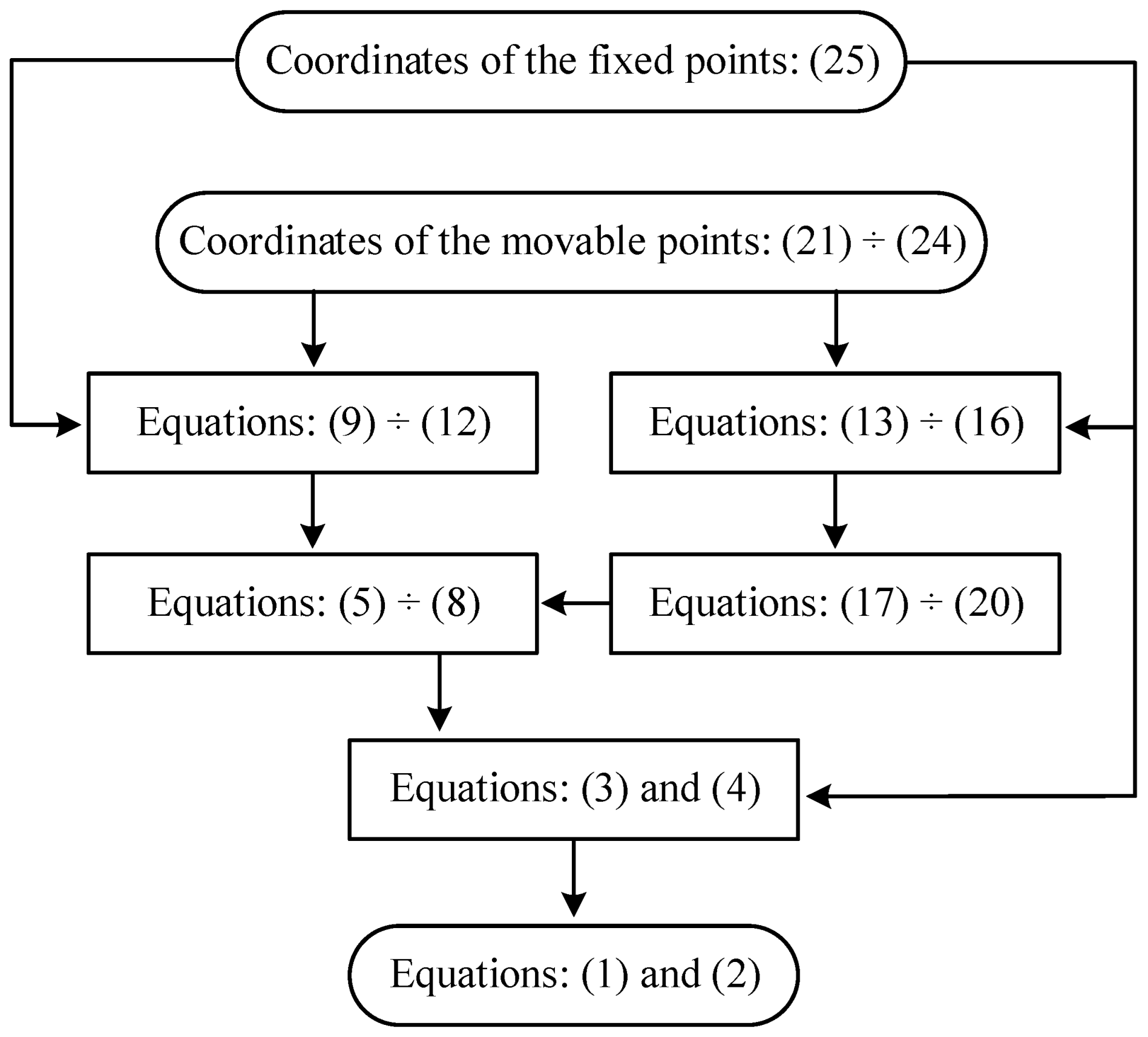
The algorithm for obtaining the highly nonlinear system of differential Equations (1) and (2), prepared for programming in MatLab ver. 6.1, is shown schematically in Figure 3.

The coordinates of the fixed points, as defined in Equation (25), and the coordinates of the moving points, as defined in Equations (21) ÷ (24), serve as inputs to Equations (9) ÷ (12) and Equations (13) ÷ (16), respectively. Additionally, the coordinates of the fixed points, as given in Equation (25), are also required to obtain Equations (3) and (4).

From the analysis of the resulting system of differential equations, it was established that an analytical solution is impossible due to the extremely large nonlinearity. Therefore, a program was compiled within the MatLab package’s programming environment. To avoid a gross error, the system of differential Equations (1) and (2) is solved using two methods: classical programming and simulation programming with the Simulink toolbox (Figure 4).

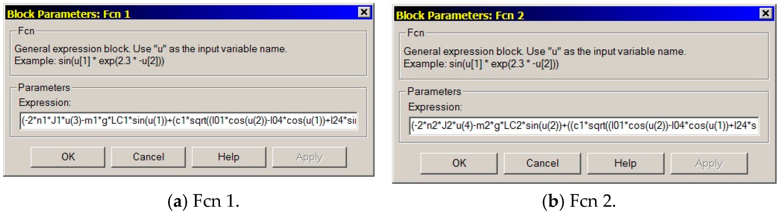
Numerical integration was performed using the fourth-order Runge–Kutta method with a fixed time step of $∆t = 0.01 \mathrm{s}$. Figure 5 shows screenshots of the Simulink model blocks Fcn 1 (a) and Fcn 2 (b) (see Figure 4). These blocks implement the final programmed equations of motion for pendulums $M_1$ and $M_2$, respectively. The equations were derived based on expressions (1) through (26) and by applying the algorithm illustrated in Figure 3.

3. Sensor Nodes and Measurement Setup

3.1. Inertial Measurement Unit

The BNO055 [29], developed by Bosch Sensortec GmbH (Reutlingen, Germany), is an intelligent sensor that combines a 3-axis accelerometer, a 3-axis gyroscope, and a 3-axis magnetometer within a single system-in-package (SiP). It also includes a 32-bit Cortex-M0 microcontroller running Bosch’s BSX3.0 FusionLib software for real-time sensor fusion. This integration enables the direct output of orientation and motion data, streamlining application development and enhancing accuracy. BNO055 is ideal for real-time monitoring applications requiring precise motion tracking, robust calibration, and seamless integration with embedded systems.

The BNO055 operates in various modes, including non-fusion (e.g., accelerometer-only, gyroscope only) and fusion modes (e.g., IMU, NDOF). The selected mode depends on the application requirements and provides data such as Euler angles, quaternions, linear acceleration, and gravity vectors.

• Interface: The sensor communicates via UART or I²C interface, with selectable slave addresses of 0x28 or 0x29.
• Power Supply: Operates within a supply voltage range of 2.4 ÷ 3.6 V.
• Sampling Frequency: Configurable, depending on the operating mode and application requirements.

The device supports automatic, real-time calibration that is continuously refined based on sensor activity and movement patterns. Calibration of the gyroscope requires the device to remain stationary for several seconds, allowing it to establish a bias reference. The accelerometer is calibrated by placing the sensor in multiple stable, static positions, ideally covering all six orthogonal orientations. The magnetometer requires dynamic motion, typically figure “∞” patterns and multi-axis rotations to compensate for hard and soft iron distortions and to establish a reliable geomagnetic reference frame. The sensor’s current calibration status can be monitored via the CALIB_STAT register, which reports individual calibration levels 0 ÷ 3 for accelerometer, gyroscope, magnetometer, and the overall system. A status of 3 indicates that the calibration is complete.

3.2. Measurement Setup

The BNO055 is mounted on a development board and interfaced with a microcontroller. It captures motion data, including acceleration, angular velocity, and magnetic field, which are transmitted wirelessly to a data acquisition system for further analysis and processing. The system utilizes the NDOF mode to deliver precise orientation measurements while minimizing drift and noise.

Two identical sensor nodes, based on the Adafruit 9-DOF Absolute Orientation IMU Fusion Breakout board, were used to investigate the developed mathematical model of the two-pendulum system experimentally. One sensor node is mounted at the center of the first pendulum $M_1.$ The other is mounted at the center of the pendulum $M_2$ (Figure 6). The sampling rate of both nodes is $80 \mathrm{H}\mathrm{z}.$ A development board based on the ESP32-C3 system-on-chip is used to transmit data to a server. The communication between it and the sensor is over the I²C interface, and the sensor has an address of $0x29.$ The power supply for each sensor node is a Li-Po battery with a capacity of $120 \mathrm{m}\mathrm{A}\mathrm{h}$ and dimensions of $4 \mathrm{m}\mathrm{m}\times 12 \mathrm{m}\mathrm{m}\times 35 \mathrm{m}\mathrm{m}.$ The system, thus implemented, enables the autonomous operation of each sensor node for approximately $40 \mathrm{m}\mathrm{i}\mathrm{n}.$ To reduce the weight of the sensor nodes, all elements necessary for charging the batteries are not mounted on them.

The weight of each sensor node, including the battery, is $12.8 \mathrm{g}.$ In the mathematical analysis, it is added to the weights of the two pendulums, $M_1$and $M_2$. The data from the sensor nodes are transmitted over different ports using the $UDP$ protocol to a server based on the LabVIEW virtual instrument, where they are recorded and visualized. The BNO055 is configured in NDOF mode, where the absolute orientation data are calculated from the accelerometer, gyroscope, and magnetometer. In this mode of operation, the ranges of all three sensors are selected by the sensor microcontroller and cannot be set by the user. The maximum sampling rates for the accelerometer and gyroscope are $100 \mathrm{H}\mathrm{z}$, while the magnetometer has a sampling rate of $20 \mathrm{H}\mathrm{z}$. In this configuration, fast magnetometer calibration is turned on.

To enable a more accurate assessment of the IMU error characteristics, an Allan deviation analysis was conducted for both the accelerometer and gyroscope. The sensors selected for this investigation are the primary sources of data for the various IMU output parameters. Notably, the accelerometer and gyroscope used in this study do not incorporate any embedded algorithms for signal stabilization or output management, which ensures the validity of such an analysis. The key value of this type of analysis lies in its ability to evaluate the system’s performance based solely on the raw output data from each sensor.

The same type of sensor node used for measuring the motion of the two pendulums was employed in this analysis. The sampling frequency was maintained at $80 \mathrm{H}\mathrm{z}$. The only difference compared to the sensor node depicted in Figure 6 is the battery capacity: for the present analysis, a $\mathrm{10,000} \mathrm{m}\mathrm{A}\mathrm{h}$ power bank was used. The sensor node, together with the battery, was placed on a vibration-isolated table and kept stationary for 6 h, during which all output data were recorded continuously.

For both sensors, the Z-axis was aligned with the direction of the gravitational acceleration $g$. All measurements reported in this publication were conducted under calibration mode 3.

Figure 7 presents the results of the Allan deviation analysis for the BNO055 accelerometer. At the sampling frequency of 80 Hz—identical to that used by the sensor node—the standard deviation for a single measurement was found to be ${\sigma }_{A{D}_{single measurement} }=0.0109 \mathrm{m}/{\mathrm{s}}^2,0.0117 \mathrm{m}/{\mathrm{s}}^2$, and $0.01633 \mathrm{m}/{\mathrm{s}}^2$ for the x, y, and z-axes, respectively (the corresponding values are indicated by dots on the graph). The mean values (MEAN) of the recorded acceleration data for the respective axes were $1.741 \mathrm{m}/{\mathrm{s}}^2,0.411 \mathrm{m}/{\mathrm{s}}^2$, and $9.577 \mathrm{m}/{\mathrm{s}}^2$.

The coefficient of variation ($CV$) is calculated using the following formula:

$$CV={\displaystyle \frac{{\sigma }_{AD}}{MEAN}} · 100.$$

(27)

For the three axes, the coefficient of variation (CV) is, respectively:

$${CV}_x=0.626\%, {CV}_y=2.847\% \mathrm{a}\mathrm{n}\mathrm{d} {CV}_z=0.171\%.$$

(28)

Figure 8 presents the results of the Allan deviation (AD) analysis for the BNO055 gyroscope. The sampling frequency was again set to 80 Hz, consistent with the frequency used in all other experiments. The standard deviation for a single measurement along the three axes was found to be:

$${\sigma }_{A{D}_x }=0.00116 \mathrm{r}\mathrm{a}\mathrm{d}/\mathrm{s}, {\sigma }_{A{D}_y }=0.00213 \mathrm{r}\mathrm{a}\mathrm{d}/\mathrm{s}\mathrm{a}\mathrm{n}\mathrm{d} {\sigma }_{A{D}_z }=0.00127 \mathrm{r}\mathrm{a}\mathrm{d}/\mathrm{s}.$$

(29)

The corresponding values are indicated by dots on the graph.

4. Results and Discussions

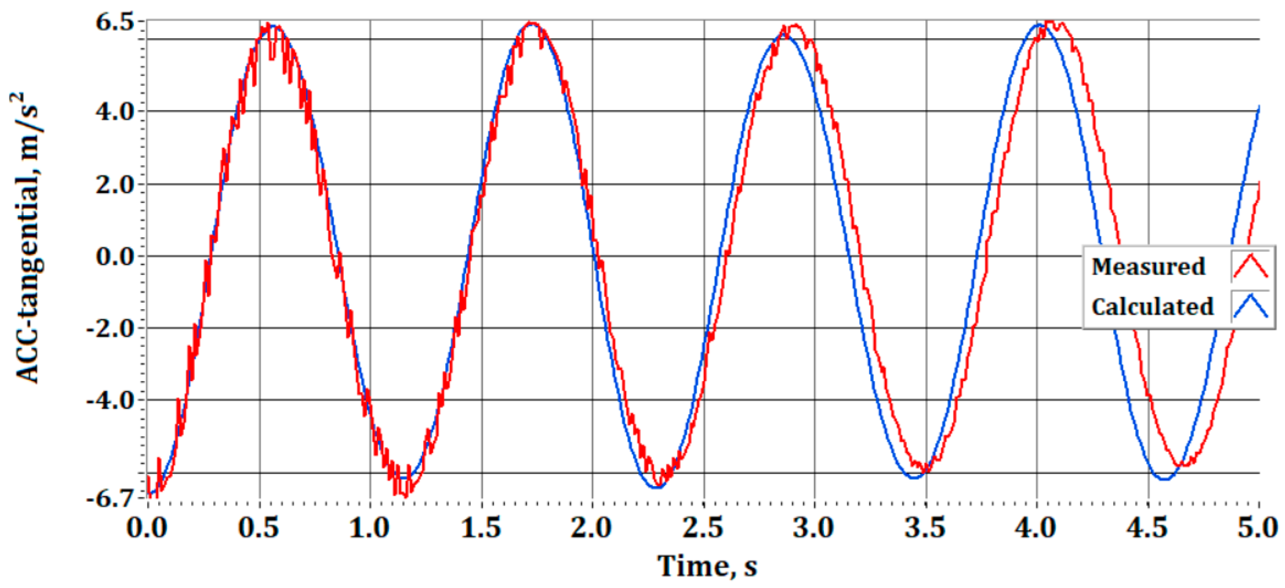
Figure 9 shows the measured and calculated tangential accelerations of the pendulum $M_1$ for the first $5$ s. The system is set in motion by deflecting pendulum $M_1$ to an angle ${\phi }_1=\pi /6 rad\equiv 30°,$ with no initial velocity. The blue graph is obtained from numerical calculations. The graph shown in red is from the experimental studies. It can be seen that there is good agreement concerning the amplitudes. In terms of frequency, the first three periods match perfectly, after which some discrepancy between the calculated and measured results can be observed. This discrepancy may be due to the mathematical model’s assumption that all mechanical connections are ideal, without considering the presence of dry friction.

Furthermore, in elastic elements (springs), there is dissipation caused by the internal friction of the material. Finally, the discrepancy can also be attributed to the numerical integration method. The natural frequency obtained from numerical integration is$f_C= 0.8601 \mathrm{H}\mathrm{z}.$ The frequency obtained from the measurements is $f_M=0.8657 \mathrm{H}\mathrm{z}.$ The relative error between the two results is $\delta =0.65\%.$

Figure 10 shows the normal accelerations of the pendulum $M_1$ for the first $5$ s. The projection of the Earth’s gravity, $g=9.81 \mathrm{m}/{\mathrm{s}}^2,$ onto the normal ${\mathrm{OK}}_1$ is added to the results (Figure 2).

The system is set in motion by deflecting pendulum $M_1$ to an angle ${\mathrm{\phi }}_1=\pi /6 rad\equiv 30°,$ with no initial velocity. Again, the blue graph shows the result obtained from the numerical calculations. The red graph shows the results obtained from experimental studies. There is a good agreement concerning the amplitudes. For the frequency, the first three periods match perfectly again, after which a discrepancy arises between the calculated and measured results.

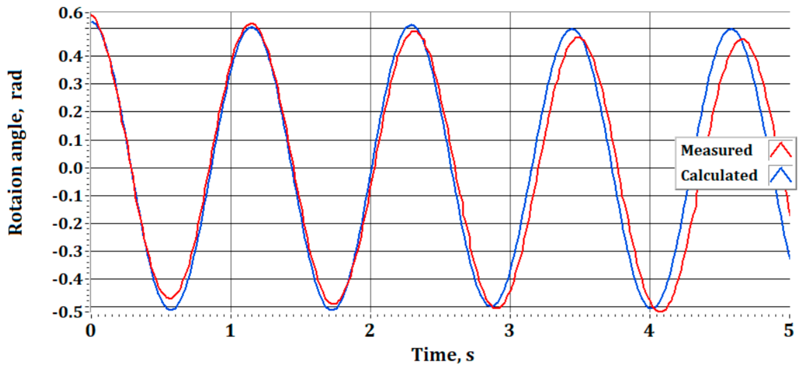
Figure 11 shows the rotation angle ${\mathrm{\phi }}_1$ of pendulum $M_1$ for the first $5$ s. Here, the experiment is started with an initial rotation angle ${\mathrm{\phi }}_1=0.593 rad (\approx 34°)$, while the initial angle in the numerical calculations is ${\mathrm{\phi }}_1=\pi /6 rad\equiv 30°.$ This leads to a minor discrepancy between the amplitudes. Again, the discrepancy between the measured and calculated natural frequencies is the same as for the accelerations, with a relative error $\delta$ of less than $1\%.$

Figure 12 shows the measured and calculated rotation angle ${\mathrm{\phi }}_1$ of pendulum $M_1$ for $120$ s.

From the two graphs shown in Figure 11 and Figure 12, it can be observed that during the first 5 s, the discrepancies between the theoretically calculated and experimentally measured results are minimal. After the tenth second, however, both pendulums $M_1$ and $M_2$ gradually begin to deviate from their plane of oscillation (Oxy). Disturbing oscillations emerge along the axis perpendicular to the Oxy plane. These disturbances are precisely what cause the occurrence of “beating” in the experimentally recorded oscillations. The increasing discrepancy over time between the computational and measured results is also due to the theoretical model’s assumption of a planar configuration (specifically, the Oxy plane, as shown in Figure 2). In reality, however, the actual system is spatial. Each pendulum moves within its plane, which is parallel to the by plane. A distance of 50 mm separates these two planes. The elastic elements between points 1–2 and 1–3, connecting pendulum $M_1$ to pendulum $M_2$ (Figure 2), induce mutual oscillations of the pendulums in a direction perpendicular to the Oxy plane. These oscillations affect the kinetic and potential energy, as well as the resistances due to internal friction in the springs and dry friction in the bearings and joints. The planar dynamic model does not capture such effects.”

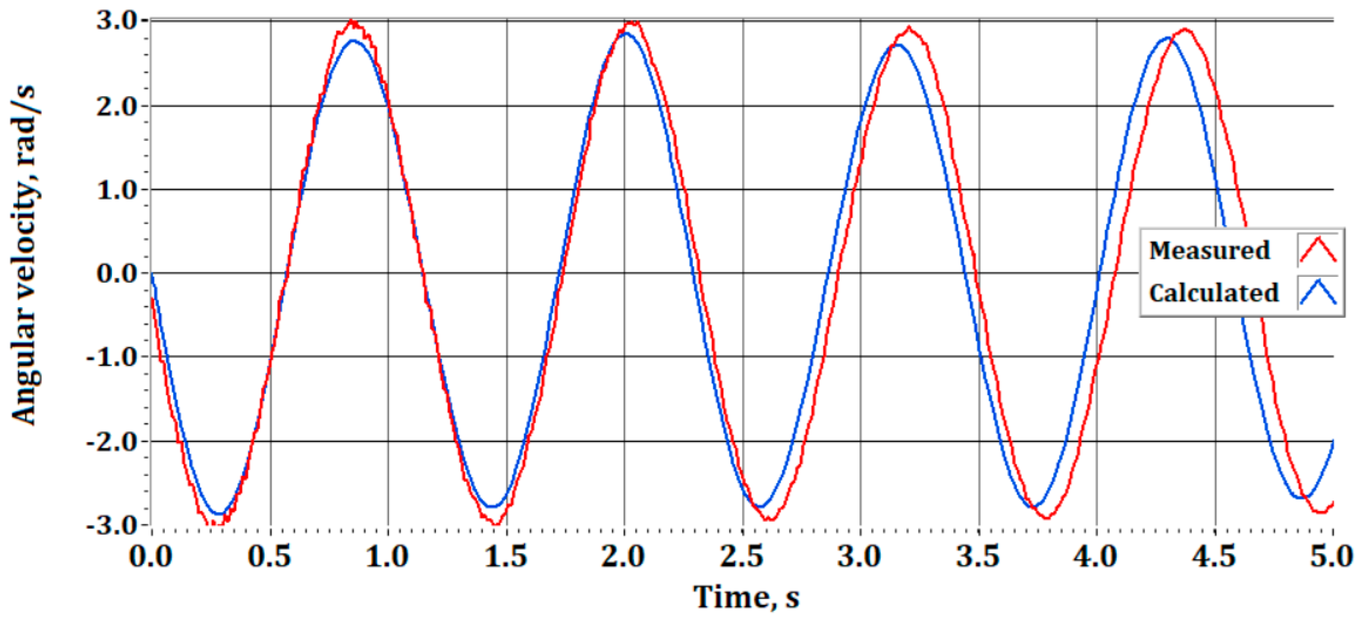
Figure 13 shows the measured and calculated angular velocity ${\mathsf{\omega }}_1{=\dot{\phi }}_1, rad/s$, of pendulum $M_1$ for the first $5$ s. The initial angular velocity is zero. The initial angle is ${\mathrm{\phi }}_1=\pi /6 rad\equiv 30°$. Again, the discrepancy between the measured and calculated frequencies and amplitudes is within the generally accepted engineering accuracy. The relative error is less than $1\%.$

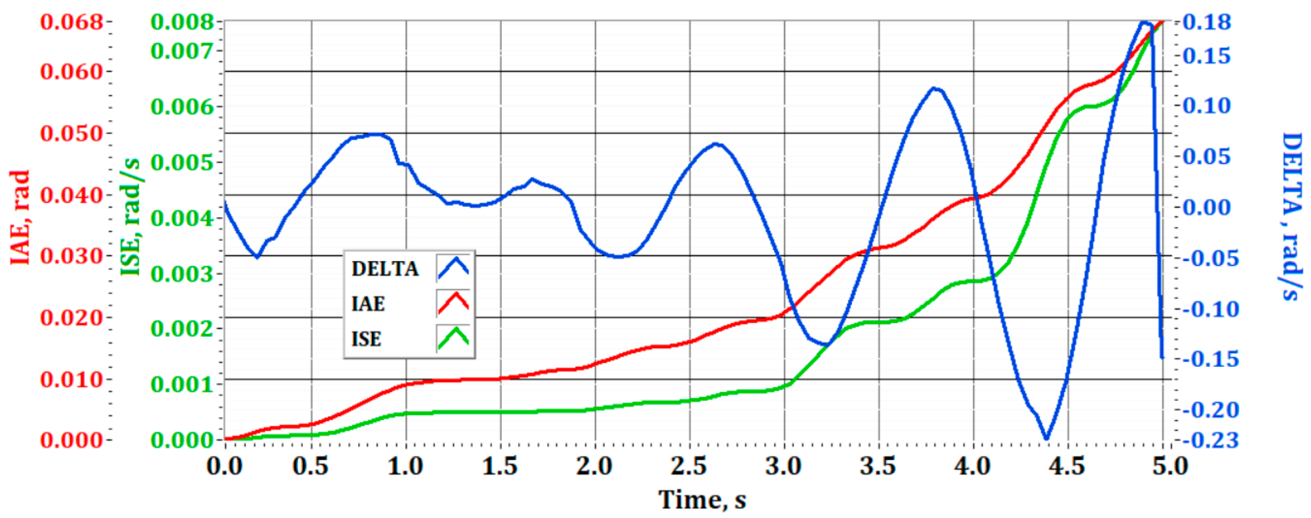
To enable a more comprehensive evaluation of the obtained results, Figure 14 presents the absolute error ($\Delta$), the Integral Absolute Error (IAE), and the Integral Square Error (ISE) over a 5 s interval. To compute all three error metrics accurately, the measured and computed angular velocities were synchronized and evaluated at the same time instances.

The absolute error at a given time $t_i, (i=\mathrm{0,1},2,\dots ,n)$ is calculated using the following formula:

$${\Delta }_i\equiv \Delta \left(t_i\right)=f_N\left(t_i\right)-f_M\left(t_i\right),$$

(30)

where $f_N\left(t_i\right)$ represents the values obtained from numerical integration, and $f_{\mathrm{M}}\left(t_i\right)$ corresponds to the values obtained from the measured data.

The Integral Absolute Error (IAE) and the Integral Square Error (ISE) were determined by numerical integration at fixed step $t_s$ over a 5 s interval using Simpson’s method, as defined by the following expressions:

$$IAE=t_s·\sum _{i=1}^n⌊e\left(t_i\right)⌋,$$

(31)

$$ISE=t_s·\sum _{i=1}^n{e\left(t_i\right)}^2.$$

(32)

The absolute error was found to lie within the range of $-0.23 \mathrm{t}\mathrm{o} 0.18 \mathrm{r}\mathrm{a}\mathrm{d}/\mathrm{s}.$

The Integral Absolute Error (IAE) at the final time point $t_n=5 \mathrm{s}$ is $0.068 \mathrm{r}\mathrm{a}\mathrm{d}.$

The Integral Square Error (ISE) at $t_n=5 \mathrm{s}$ is $0.008 \mathrm{r}\mathrm{a}\mathrm{d}/\mathrm{s}$.

The analysis of the error metrics obtained demonstrates a strong correlation between the theoretically predicted outcomes and the experimentally measured data. The studied mechanical system exhibits a tendency toward a stable equilibrium state. As the oscillations progressively decay, the integral performance indices, IAE and ISE, increase until the oscillatory behavior is fully damped.

Figure 15 shows the plot of the angular velocities of pendulum $M_2$ calculated and measured for $120$ s. Here, the differences between the calculated and measured values are larger. The primary reason for this is that the model assumes all mechanical connections are ideal. In the experimental rig used, there are no bearing connections at spring joints 2, 3, and 5 (Figure 2). Furthermore, the dynamical model is built in a 2D plane, $Oxy.$ The actual model is spatial, as the two pendulums are spaced $23 \mathrm{m}\mathrm{m}$ apart. Springs 1–2 and 1–3 (Figure 2) are located at an angle to the $Oz$ axis, which is not shown in the planar drawing.

5. Conclusions

This study presents a comprehensive numerical and experimental investigation of the nonlinear oscillations of a coupled two-pendulum mechanical system. The system exhibits strong geometric and dynamic nonlinearities due to large angular displacements, elastic couplings, and internal damping, which prevent the derivation of closed-form analytical solutions. To address these complexities, a detailed mathematical model was developed in the MatLab/Simulink environment, incorporating gravitational, inertial, and nonlinear elastic restoring forces, as well as damping coefficients experimentally identified through logarithmic decrement analysis.

The main findings and contributions can be summarized as follows:

• Development of a High-Fidelity Numerical Model:

A stable mathematical framework was developed for modelling the nonlinear oscillatory behavior of a two-mass system. The system of governing differential equations was derived based on the laws of Newtonian mechanics and solved using the fourth-order Runge–Kutta method. Particular attention was paid to accurately accounting for the effect of elastic coupling and experimentally determined damping forces.

• Experimental Validation Using High-Precision Inertial Sensors:

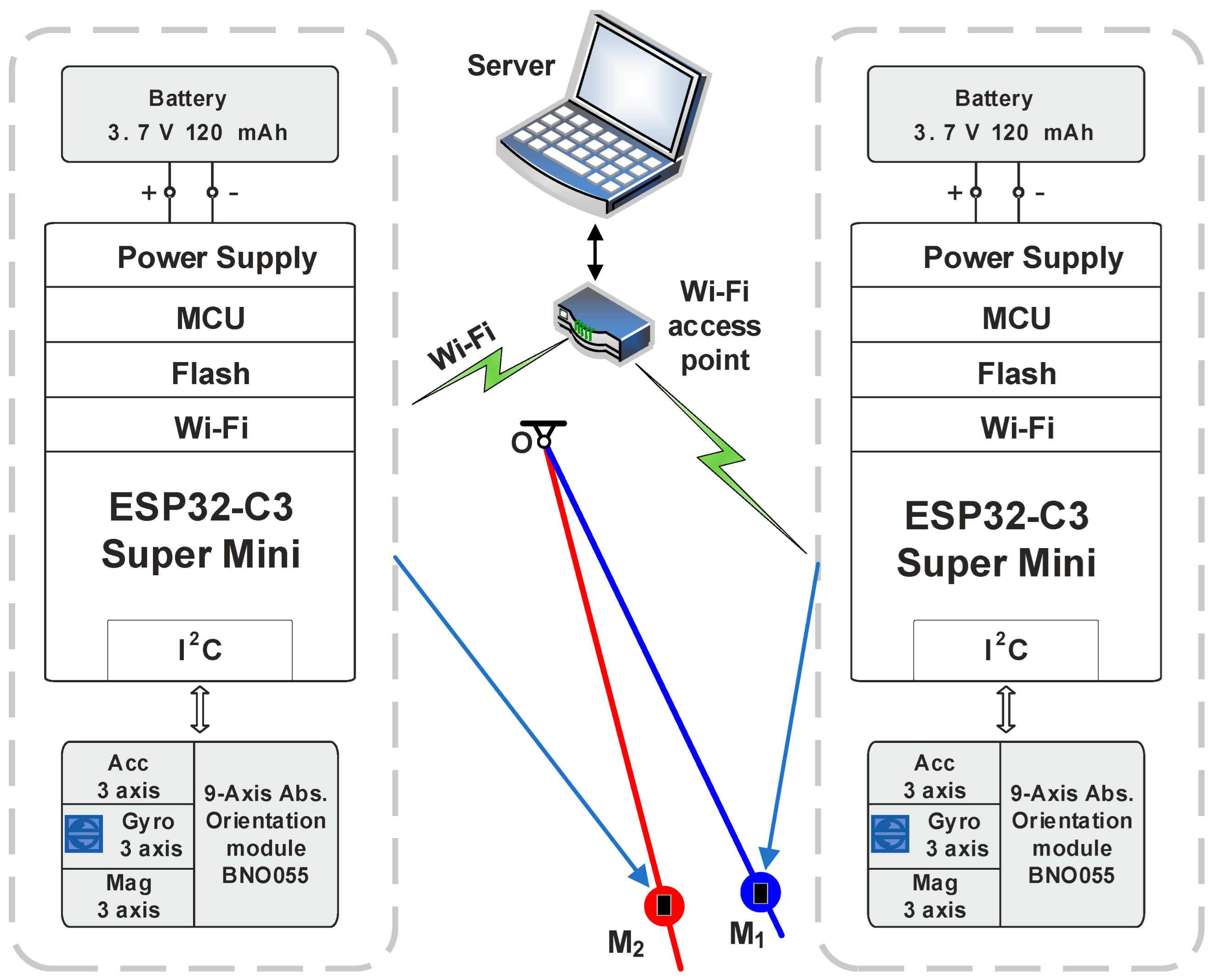
The dynamic responses of both pendulums were measured using BNO055-based sensor nodes configured in NDOF mode. The sensor nodes enabled the real-time acquisition of angular positions, accelerations, and velocities. The experimental results demonstrated excellent agreement with numerical simulations in terms of amplitude decay and natural frequency, with relative errors of less than 1% during the initial oscillation intervals.

• Characterization of sensors and quantitative assessment of errors:

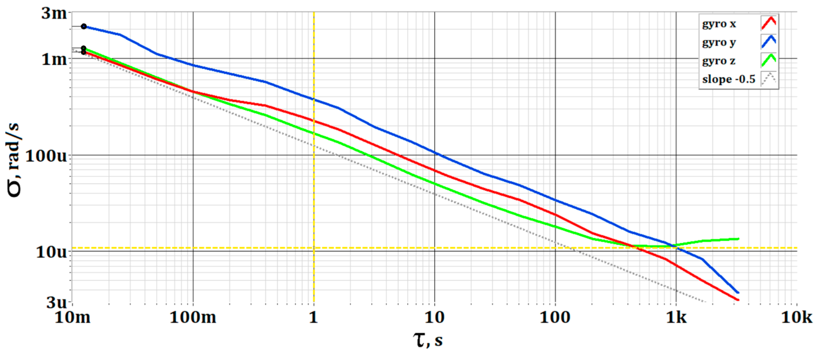
To ensure data reliability, an analysis of Allan deviation was conducted for the IMU sensors under static conditions. Standard deviations and coefficients of variation were determined for all axes, confirming the reliability of the sensor data. In addition, a detailed error analysis was performed, including absolute error, Integral Absolute Error (IAE) and Integral Square Error (ISE), based on synchronized time series for a 5 s interval. The maximum absolute error remained within the range from −0.23 to 0.18 rad/s, while the IAE and ISE values were minimal, demonstrating the model’s predictive accuracy.

• Assessment of planar and spatial dynamics:

Although the model assumes a planar configuration, the experimental results revealed deviations due to spatial effects, in particular out-of-plane oscillations and beating phenomena observed after prolonged motion. These discrepancies are explained by the physical displacement between the planes of the pendulum and the three-dimensional orientation of the connecting springs. This highlights the need for future expansion of the model to account for three-dimensional dynamics and the effects of spatial coupling.

• Scientific and Applied Impact:

The hybrid analytical and experimental methodology presented in this study offers a validated approach for investigating nonlinear multibody systems with elastic couplings. The framework is extendable to forced and parametrically excited oscillations and has practical implications for structural dynamics, vibration control, and mechatronic system design. The experimental setup and modeling tools provide a solid foundation for future research in the areas of resonance control, synchronization, and spatial modeling of complex oscillatory systems.

Building on the current results, future research will explore forced excitation regimes, including chaotic and resonant behaviors, as well as the synchronization dynamics of the coupled pendulums. Another key direction will be the development of a fully spatial, dynamic model that captures all degrees of freedom, further improving the fidelity of simulation outcomes. These developments will expand the applicability of the framework to advanced domains such as robotics, structural health monitoring, and adaptive control systems.