Decoupled Reinforcement Hybrid PPO–Sliding Control for Underactuated Systems: Application to Cart–Pole and Acrobot

Abstract

Underactuated systems, such as the Cart–Pole and Acrobot, pose significant control challenges due to their inherent nonlinearity and limited actuation. Traditional control methods often struggle to achieve stable and optimal performance in these complex scenarios. This paper presents a novel stable reinforcement learning (RL) approach for underactuated systems, integrating advanced exploration–exploitation mechanisms and a refined policy optimization framework to address instability issues in RL-based control. The proposed method is validated through extensive experiments on two benchmark underactuated systems: the Cart–Pole and Acrobot. In the Cart–Pole task, the method achieves long-term balance with high stability, outperforming traditional RL algorithms such as the Proximal Policy Optimization (PPO) in average episode length and robustness to environmental disturbances. For the Acrobot, the approach enables reliable swing-up and near-vertical stabilization but cannot achieve sustained balance control beyond short time intervals due to residual dynamics and control limitations. A key contribution is the development of a hybrid PPO–sliding mode control strategy that enhances learning efficiency and stabilities for underactuated systems.

1. Introduction

Reinforcement learning (RL) has emerged as a transformative paradigm in artificial intelligence (AI), enabling agents to learn optimal behaviors through interaction with environments and feedback in the form of rewards [1]. Rooted in behaviorist psychology and formalized through Markov decision processes (MDPs), RL has evolved from theoretical foundations to practical applications across robotics, gaming, healthcare, and beyond [2,3,4]. Computational implementations emerged in the 1950s with Arthur Samuel’s checkers playing program, but modern RL frameworks were formalized in the 1980s with the introduction of temporal difference (TD) learning and Q-Learning [5,6]. The integration of deep learning in the 2010s, exemplified by the DeepMind’s Deep Q-Network (DQN) achieving human-level performance in Atari games, marked a pivotal shift toward solving complex, high-dimensional problems [7].

RL is a subfield of machine learning that focuses on how an intelligent agent can learn to make optimal decisions in an environment to maximize a cumulative reward. It differs from other machine learning paradigms such as supervised learning (which relies on labeled data) and unsupervised learning (which focuses on finding patterns in unlabeled data) by its emphasis on learning through interaction with the environment. RL has seen significant growth in recent years, driven by both theoretical advancements and practical applications in areas like robotics, gaming, and autonomous systems. RL algorithms are categorized into (1) Value-Based Methods: estimate the optimal action values (e.g., Q-Learning and Deep Q-Network (DQN)) [6,7]; (2) Policy-Based Methods: directly optimize policies (e.g., Policy Gradients and Trust Region Policy Optimization (TRPO)) [8,9]; (3) Actor–Critic Methods: combine value and policy learning (e.g., Asynchronous Advantage Actor–Critic (A3C) and Proximal Policy Optimization (PPO)) [10,11].

Hybrid reinforcement learning–classical control frameworks have been explored in prior studies, such as the combination of reinforcement with model predictive control for manipulators [12] and the integration of the State-Dependent Riccati Equation with PID control for quadrotor stabilization [13]. However, these approaches typically adopt a single-stage control paradigm where RL and classical controllers operate in parallel or with static weightings, which may struggle with the nonlinear dynamics of underactuated systems. In contrast, the proposed PPO–SMC framework introduces a two-stage adaptive switching strategy: PPO learns the swing-up dynamics from scratch without model knowledge, while SMC ensures Lyapunov-stable stabilization near the equilibrium. The novelty lies in the synergistic design, where PPO’s data-driven exploration addresses the swing-up challenge of model-based methods, and SMC’s theoretical guarantees overcome the stability limitations of pure RL.

The Cart–Pole and Acrobot are canonical benchmarks for underactuated control systems, each exhibiting unique challenges in stabilization. The Cart–Pole consists of a cart moving horizontally with a pendulum attached, controlled by applying forces to the cart [14,15]. In contrast, the Acrobot is a two-link robotic arm with only the second joint actuated [15,16]. Both systems require precise control to maintain unstable equilibrium positions, but their distinct dynamics necessitate tailored control strategies.

This paper presents a hybrid control framework combining PPO and Sliding Mode Control (SMC) [17,18,19] for the Cart–Pole system and compares it with the Acrobot implementation. To evaluate the hybrid framework across varying system complexities, we apply it to two canonical benchmarks: Cart–Pole (single-link, position–angle coupling) and Acrobot (two-link, fully coupled angular dynamics). While PPO alone suffices for Cart–Pole, the hybrid approach demonstrates enhanced robustness and efficiency, providing a baseline for its application to the more challenging Acrobot. We demonstrate how the hybrid approach leverages PPO for swing-up and SMC for stabilization in both systems while highlighting key differences in model structure and control design.

The Acrobot, a planar two-link robotic arm operating in the vertical plane, has emerged as a significant subject of study in the field of robotics, particularly in the realm of underactuated systems. It is characterized by having an actuator at the elbow joint (the second joint), while the shoulder joint (the first joint) remains unactuated. This underactuated nature poses unique challenges and opportunities in terms of control and dynamic analysis.

The study of the Acrobot’s mathematical model is crucial for several reasons. Firstly, it enables a profound understanding of the system’s behavior, including its motion patterns, energy transfer mechanisms, and stability characteristics. Secondly, it provides a solid foundation for the design and implementation of effective control algorithms. By accurately describing the relationship between the system’s inputs (actuating torque at the elbow) and its outputs (link angular displacements and velocities), control strategies can be developed to achieve desired tasks, such as the swing-up and balance control of the Acrobot.

This paper presents a PPO framework for stabilizing the Acrobot, a classic underactuated robotic system, in its upright equilibrium position. By formulating the control problem as a MDP, we design a PPO agent to learn feedback control policies directly from interaction with the system. The Acrobot’s underactuated nature (with only the elbow joint actuated) poses significant challenges for traditional control methods, which often require full-state feedback and precise model knowledge. Reinforcement learning (RL), particularly model-free algorithms like PPO, offers a data-driven alternative to learn control policies without explicit dynamics modeling. However, RL-based control lacks traditional stability guarantees, necessitating a hybrid approach that merges empirical training with theoretical analysis.

Policy gradient methods in RL optimize a parameterized policy ${\pi }_{\theta }(a|\mathrm{s})$ by directly estimating the gradient of the expected cumulative reward. The ${\pi }_{\theta }(a|\mathrm{s})$ represents the probability of taking action $a$ when in state $\mathrm{s}$ under the policy with parameters $\theta$. However, traditional policy gradient algorithms like Reinforce [20] and Actor–Critic [21,22] often suffer from instability due to large policy updates, which can lead to performance degradation or divergence. PPO [23] addresses this issue by formulating policy optimization as a constrained problem, ensuring that each policy update remains “close” to the previous policy. This approach balances exploration and exploitation while maintaining stable training, making PPO one of the most widely used RL algorithms in practice.

This paper presents a hybrid control strategy combining PPO, a deep reinforcement learning (DRL) algorithm, with SMC for stabilizing the Acrobot, a challenging underactuated robotic system. The proposed approach leverages PPO’s exploration capabilities to swing the Acrobot up to a near-vertical state, then switches to a custom sliding mode controller to achieve precise stabilization. Stability analysis based on Lyapunov theory confirms the closed-loop system’s convergence to the desired equilibrium.

Section 4 presents a hybrid control framework combining PPO and SMC for stabilizing the Cart–Pole and Acrobot systems. Leveraging OpenAI Gym [24] for simulation and TensorFlow [25] for neural network implementation, we demonstrate that the hybrid approach outperforms standalone PPO or SMC in both swing-up efficiency and stabilization accuracy. Detailed simulation results validate the robustness of the proposed method under varying initial conditions. Simulation results demonstrate that the hybrid controller outperforms standalone PPO or SMC in both swing-up efficiency and stabilization accuracy.

2. Mathematic Model

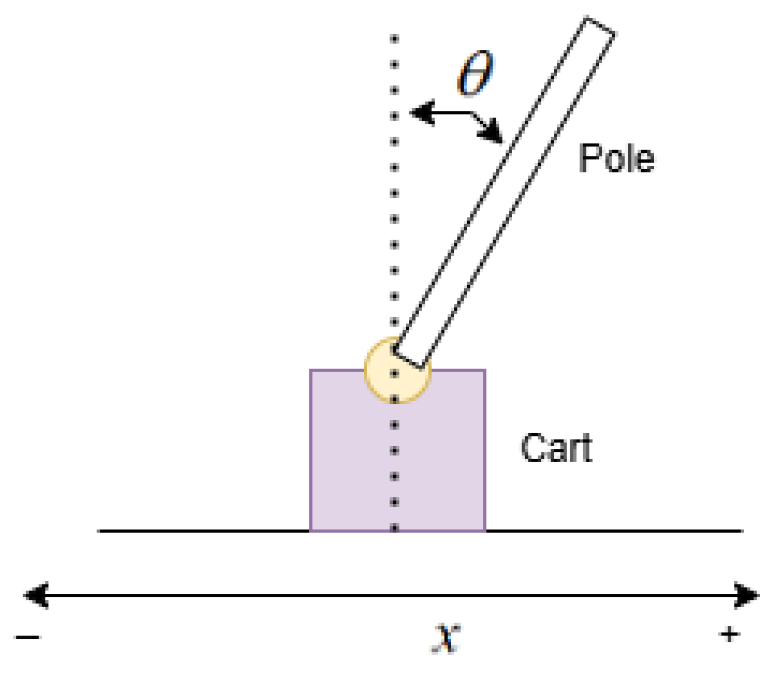
2.1. Model of Cart–Pole

The Cart–Pole system (Figure 1) is a well-studied example in control theory. It can be modeled using Newton’s laws of motion or the Lagrangian approach. One common way to derive its equations of motion is based on the work of [3], where the following equations govern the system [15]:

$$(m_c+m_p)\ddot{x}+m_{p}l\ddot{\theta }\cos \theta -m_{p}l{\dot{\theta }}^2\sin \theta =F$$

(1)

$$m_{p}l\ddot{x}\cos \theta +m_p{l}^2\ddot{\theta }+m_{p}gl\sin \theta =0$$

(2)

where $m_c=1$ kg and $m_p=0.5\mathrm{kg}$ are the masses of the cart and pole, respectively.$m_c$ represents the mass of the cart that moves horizontally, and $m_p$ is the mass of the pole attached to the cart.

$x$ and $\theta$ are the cart position and pole angle. $x$ describes the horizontal displacement (unit is cm) of the cart along a linear track, and $\theta$ is the angle the pole makes with the vertical axis (unit is deg).

$l$ is the pole length, which is a fixed geometric parameter of the system. The unit is cm in this paper: $l=50\mathrm{cm}$.

$F$ is the control force applied to the cart, which is the input that the controller manipulates to balance the pole. The unit is N.m.

State Space: The state of the Cart–Pole system is represented by $s=\left[\begin{array}{cccc}x& \dot{x}& \theta & \dot{\theta }\end{array}\right]$. Here, $x$ and $\theta$ are the position and angle as defined above, and $\dot{x}$ and $\dot{\theta }$ are their respective time derivatives, representing the velocity of the cart and the angular velocity of the pole.

Control Input: $F$ (continuous force). The controller can apply a continuous variable force to the cart in the horizontal direction, either in the positive or negative $x$ direction. The diagram of Cart–Pole architecture is shown in Figure 1.

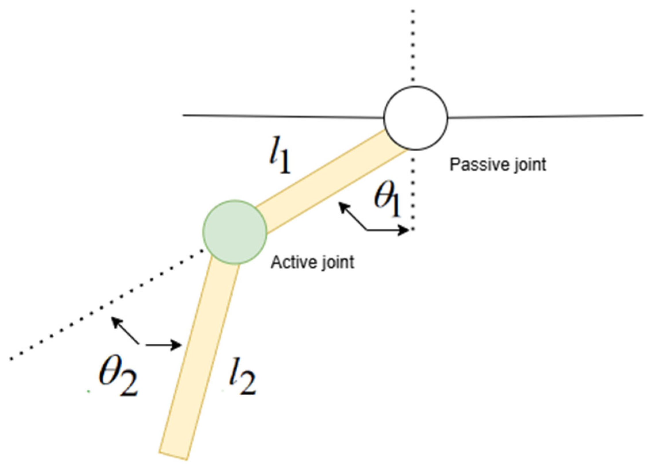
2.2. Model of Acrobot

The Acrobot’s physical characteristics are defined by a set of parameters, which are essential for constructing its mathematical model [15].

$m_1$ and $m_2$ represent the masses of the first (shoulder) and second (elbow) links, respectively. These masses influence the inertial properties of the links and play a significant role in determining the system’s kinetic energy and dynamic response to external forces. The unit is kg; in this paper, both are 1 kg.

$l_1$ and $l_2$ denote the lengths of the first and second links. The lengths affect the geometric configuration of the Acrobot and are involved in calculating the potential energy due to gravity, as well as in determining the velocities of the link centers of mass. The unit is cm; in this paper, both are 50 cm.

$I_1$ and $I_2$ signify the moments of inertia of the first and second links about their respective centers of mass. The moments of inertia quantify the resistance of the links to rotational motion and are crucial in the calculation of the system’s kinetic energy. In this paper, both are 0.1667 $\mathrm{k}\mathrm{g}\cdot {\mathrm{m}}^2$.

$g$ represents the gravitational acceleration ($g=9.8 \mathrm{m}/{\mathrm{s}}^2$), which is a constant factor in the model and has a substantial impact on the potential energy and the overall dynamic behavior of the Acrobot, especially when considering the links’ motion against gravity.

${\theta }_1$ and ${\theta }_2$ denote the angular displacements of the first and second links. The zero configuration is typically defined as when both links point directly downwards, and positive angular displacements are measured counterclockwise. These angles are the primary state variables that describe the Acrobot’s configuration in the plane. The unit is deg.

${\dot{\theta }}_1$ and ${\dot{\theta }}_2$ represent the angular velocities of the first and second links, which are the timederivatives of the angular displacements. They are essential for calculating the kinetic energy of the system and for understanding the rate of change of the Acrobot’s configuration. The unit is $\mathrm{deg}/s$.

$\tau$ signifies the actuating torque applied at the elbow joint (the second joint), which serves as the control input to the system. The unit is N.m. The ability to control the Acrobot’s motion depends on how this torque is applied and regulated. The diagram of Acrobot architecture is shown in Figure 2.

The kinetic energy of the Acrobot is composed of the translational and rotational kinetic energies of its two links.

For the first link, the kinetic energy $T_1$ is given by

$$T_1={\displaystyle \frac{1}{2}}{I}_1{\dot{\theta }}_1^2+{\displaystyle \frac{1}{2}}{m}_1{v}_{c1}^2$$

(3)

where $v_{c1}$ is the velocity of the center of mass of the first link. Considering the geometric relationship, $v_{c1}=l_{c1}{\dot{\theta }}_1$ (where $l_{c1}$ is the distance from the shoulder joint to the center of mass of the first link), so

$$T_1={\displaystyle \frac{1}{2}}(I_1+m_1{l}_{c1}^2){\dot{\theta }}_1^2$$

(4)

For the second link, the kinetic energy $T_2$ is more complex due to the combined effects of the shoulder and elbow joint motions. The position of the center of mass of the second link in Cartesian coordinates is

$${\mathit{p}}_{c2}=\left[\begin{array}{c}{l}_1\sin {\theta }_1+l_{c2}\sin ({\theta }_1+{\theta }_2)\\ -l_1\cos {\theta }_1-l_{c2}\cos ({\theta }_1+{\theta }_2)\end{array}\right]$$

(5)

The velocity of the center of mass of the second link ${\mathit{v}}_{c2}={\displaystyle \frac{d{\mathit{p}}_{c2}}{dt}}$, and after some calculations, the kinetic energy of the second link is

$$T_2={\displaystyle \frac{1}{2}}{m}_2{v}_{c2}^2+{\displaystyle \frac{1}{2}}{I}_2{({\dot{\theta }}_1+{\dot{\theta }}_2)}^2$$

(6)

where $v_{c2}^2={ \dot{\mathit{p}}}_{c2}^T{ \dot{\mathit{p}}}_{c2}$. Expanding and simplifying, we obtain

$$T_2={\displaystyle \frac{1}{2}}(m_2(l_1^2+l_{c2}^2+2l_1{l}_{c2}\cos {\theta }_2)+I_2){\dot{\theta }}_1^2+{\displaystyle \frac{1}{2}}{I}_2{\dot{\theta }}_2^2+(I_2+m_2{l}_1{l}_{c2}\cos {\theta }_2){\dot{\theta }}_1{\dot{\theta }}_2$$

(7)

The total kinetic energy of the Acrobot $T=T_1+T_2$ can be written in matrix form as $T={\displaystyle \frac{1}{2}}{\dot{\mathit{\theta }}}^T\mathit{M}(\mathit{\theta })\dot{\mathit{\theta }}$, where $\dot{\mathit{\theta }}=\left[\begin{array}{c}{\dot{\theta }}_1\\ {\dot{\theta }}_2\end{array}\right]$, and the inertia matrix $\mathit{M}(\mathit{\theta })$ is given by

$$\mathit{M}(\mathit{\theta })=\left[\begin{array}{cc}{I}_1+I_2+m_1{l}_{c1}^2+m_2(l_1^2+l_{c2}^2+2l_1{l}_{c2}\cos {\theta }_2)& I_2+m_2{l}_1{l}_{c2}\cos {\theta }_2\\ I_2+m_2{l}_1{l}_{c2}\cos {\theta }_2& I_2\end{array}\right]$$

(8)

The potential energy of the Acrobot is due to the gravitational force acting on the two links. The potential energy of the first link $V_1=m_{1}g{h}_{c1}$,where $h_{c1}=-l_{c1}\cos {\theta }_1$, so

$$V_1=-m_{1}g{l}_{c1}\cos {\theta }_1$$

(9)

The potential energy of the second link $V_2=m_{2}g{h}_{c2}$, where $h_{c2}=-(l_1\cos {\theta }_1+l_{c2}\cos ({\theta }_1+{\theta }_2))$, so $V_2=-m_{2}g(l_1\cos {\theta }_1+l_{c2}\cos ({\theta }_1+{\theta }_2))$.

The total potential energy is

$$V=V_1+V_2=-g[m_1{l}_{c1}\cos {\theta }_1+m_2(l_1\cos {\theta }_1+l_{c2}\cos ({\theta }_1+{\theta }_2))]$$

(10)

The Lagrangian function $L$ is defined as the difference between the total kinetic energy $T$ and the total potential energy $V$, i.e., $L=T-V$.

Substituting the expressions for $T$ and $V$ obtained above, we obtain

$$L={\displaystyle \frac{1}{2}}{\dot{\mathit{\theta }}}^T\mathit{M}(\mathit{\theta })\dot{\mathit{\theta }}+g[m_1{l}_{c1}\cos {\theta }_1+m_2(l_1\cos {\theta }_1+l_{c2}\cos ({\theta }_1+{\theta }_2))]$$

(11)

The dynamic equations of the Acrobot are derived using the Euler–Lagrange equations:

$${\displaystyle \frac{d}{dt}}({\displaystyle \frac{\partial L}{\partial {\dot{\theta }}_i}})-{\displaystyle \frac{\partial L}{\partial {\dot{\theta }}_i}}={\tau }_i$$

(12)

where $i=1,2$ and ${\tau }_1=0$ (since there is no actuator at the first joint) and ${\tau }_2=\tau$ (the actuating torque applied at the second joint).

In matrix form, the dynamic model of the Acrobot can be written as

$$\mathit{M}(\mathit{\theta })\ddot{\mathit{\theta }}+\mathit{C}(\mathit{\theta },\dot{\mathit{\theta }})\dot{\mathit{\theta }}+\mathit{G}(\mathit{\theta })=\mathsf{\tau }$$

(13)

where $\mathit{C}(\mathit{\theta },\dot{\mathit{\theta }})$ is the Coriolis and centrifugal force matrix, $\mathit{G}(\mathit{\theta })$ is the gravitational force vector, and $\mathit{\tau }={\left[\begin{array}{cc}0& \tau \end{array}\right]}^T$. The dimensions of the matrices are $\mathit{M}(\mathit{\theta })\in R^{2\times 2}$, $\mathit{C}(\mathit{\theta },\dot{\mathit{\theta }})\in R^{2\times 1}$, and $\mathit{G}(\mathit{\theta })\in R^{2\times 1}$.

3. Hybrid PPO–Sliding Mode Controller Design

The Acrobot, a two-link underactuated robot with a single actuated joint, serves as a canonical benchmark for underactuated control. Its stabilization in the upright position is non-trivial due to its inherent nonlinearity and lack of full actuation. Traditional control methods like PID or SMC require precise system modeling and may struggle with swing-up dynamics, while DRL methods like PPO can learn effective swing-up policies but often lack the precision for the final stabilization. This work addresses this gap by proposing a two-stage hybrid control framework:

• PPO for Swing-Up: Learns a policy to swing the Acrobot from the hanging state to a near-vertical state.
• SMC for Stabilization: Takes over to stabilize the system at the exact vertical equilibrium, leveraging its robustness to model uncertainties.

The controller switches from PPO to SMC when

$$\mathrm{verticality}={\displaystyle \frac{-\cos {\theta }_1-\cos ({\theta }_1+{\theta }_2)}{2}}>0.9$$

(14)

This threshold ensures the Acrobot is sufficiently close to the vertical state for SMC to take over. This verticality metric quantifies the cosine of the angle between the Acrobot and the vertical axis, with a value of 1 indicating a perfect upright position.

The Acrobot’s state is defined as $\mathit{s}=\left[\begin{array}{cccc}{\theta }_1& {\theta }_2& {\dot{\theta }}_1& {\dot{\theta }}_2\end{array}\right]$. The action is the torque applied to the elbow joint. To encourage upright stabilization, the reward is designed as

$$r(\mathit{s})=-({\alpha }_1(1-\cos {\theta }_1)+{\alpha }_2{\theta }_2^2+{\alpha }_3{\dot{\theta }}_1^2+{\alpha }_4{\dot{\theta }}_2^2)$$

(15)

where ${\alpha }_i>0$ are weights. The term $(1-\cos {\theta }_1)$ penalizes deviations from ${\theta }_1=\pi$ (upright), while quadratic terms penalize joint angle/velocity errors.

The PPO algorithm optimizes the policy ${\pi }_{\theta }(a|\mathit{s})$ by maximizing the expected discounted return:

$$J(\theta )={{\rm E}}_{s_t~{\pi }_{\theta }}[{\displaystyle \sum _0^{\infty }{\gamma }^{t}r(}{\mathit{s}}_t)]$$

(16)

where $\gamma \in [0,1)$ is the discount factor. ${{\rm E}}_{s_t~{\pi }_{\theta }}$ is the expectation operator over all possible trajectories of states and actions. ${\displaystyle \sum _0^{\infty }{\gamma }^{t}r(}{\mathit{s}}_t)$ is the sum of rewards over an infinite horizon (all time steps from the start of an episode onward).

The policy is parameterized as a Gaussian distribution over torques:

$${\pi }_{\theta }(\tau |\mathit{s})=N(\mu (\mathit{s};\theta ),{\sigma }^2\mathit{I})$$

(17)

It represents the probability of taking action $a$ when in state $\mathit{s}$ under the policy with parameters $\theta$. In reinforcement learning, the policy defines how the agent acts in different states. The $\mu (\mathit{s};\theta )$ is the mean of the Gaussian distribution computed by a neural network (2 hidden layers, ReLU activations). The $\sigma$ is the lowercase letter, and it represents the standard deviation of the Gaussian distribution. It quantifies the “spread” or “dispersion” of the action distribution around the mean value $\mu$. $\mathit{I}$ denotes the identity matrix. In the covariance matrix ${\sigma }^2\mathit{I}$, the identity matrix ensures that the Gaussian distribution is axis-aligned (i.e., the action dimensions are independent of each other). For a single-dimensional action space (e.g., torque in Acrobot control), $\mathit{I}$ reduces to the scalar value 1, and the covariance matrix becomes ${\sigma }^2$. The algorithm of PPO is as follows:

Input:

• The environment E with its state space S and action space A.
• A policy network with some parameters that decides actions given states.
• A value network with some parameters that estimates state values.
• Hyperparameters: discount factor, clipping parameter, learning rates, number of update episodes, and batch size.

Output: Optimized policy parameters that perform well in the environment

Algorithm Steps:

• Initialization: Set initial values for the policy network parameters and the value network parameters.
• Outer Training Loop: Repeat the following steps for multiple iterations:
• Collecting Trajectories:

Run the environment multiple times (for N rollouts).

• In each rollout:
• Start from an initial state.
• For each time step:

Use the current policy to sample an action.

Execute the action in the environment and observe the reward and the next state.

Calculate the advantage of the action taken.

Store the state, action, reward, next state, advantage, and the probability of taking that action under the current policy.

4.

Policy Update:

• Split the collected data into smaller batch sizes.
• For each batch:
• Run many episodes of updates:

Compute the ratio of the new policy’s action probability to the old policy’s action probability.

Clip this ratio to prevent the policy from changing too much at once.

Update the policy network’s parameters to increase the likelihood of actions that lead to higher advantages while staying close to the old policy.

5.

Value Function Update:

• For each batch of collected data:

Calculate the difference between the predicted state value by the value network and the actual return (total discounted rewards).

Update the value network’s parameters to reduce this difference.

6.

Old Policy Update:

Copy the current policy’s parameters to the old parameters. This saved policy will be used in the next iteration to compare with the updated policy.

7.

End of the Outer Loop:

Repeat the process until the policy converges or meets a predefined stopping condition. The final policy’s parameter is considered the optimized policy parameters.

Training details are as follows:

• State Normalization: States are normalized using the running mean and variance to improve training stability.
• Reward Shaping: A small positive reward (+0.1) is given when ${\theta }_1$ deviates by less than $5^{\circ }$ from $\pi$, accelerating convergence.
• Hyperparameters: Batch size = 2048, episodes per update = 10, learning rate =$3\times {10}^{-4}$, and $\gamma =0.99$.

For each joint, a second-order sliding surface is designed as

$$s_i={\dot{e}}_i+{\lambda }_i{e}_i$$

(18)

where $e_i={\theta }_i-{\theta }_i^d$ is the tracking error of the angle (${\theta }_i^d$ is the target angle). ${\lambda }_i$ is a parameter of the sliding surface, determining the convergence rate of the system state to the sliding surface. For the Acrobot system, the total sliding surface is defined as a weighted sum of the sliding surfaces of the two joints:

$$s={\alpha }_1{s}_1+{\alpha }_2{s}_2$$

(19)

where the weights ${\alpha }_1=0.7$ and ${\alpha }_2=0.3$ reflect that the first joint has a greater impact on the overall stability.

The control law is designed using an exponential reaching law:

$$\tau =-{\displaystyle \sum _{i=1}^2{K}_i{s}_i-\eta \cdot sat(s/\phi )}$$

(20)

where $K_i$ are sliding mode gains, determining the motion characteristics of the system state on the sliding surface. $\eta >0$ is a robustness gain to handle system uncertainties and external disturbances. $sat(x)$ is a saturation function, which has a boundary layer thickness, used to replace the traditional sign function to reduce chattering. $\phi >0$ is the thickness parameter of the boundary layer.

The closed-loop system governed by the SMC law is globally stable if $K_i>0$ and $\eta >{‖\Delta ‖}_{\infty }$, where $\Delta$ denotes bounded uncertainties.

Using Lyapunov stability theory, we select the Lyapunov function:

$$V(s)={\displaystyle \frac{1}{2}}{s}^2$$

(21)

Its derivative is

$$\dot{V}(s)=s\cdot \dot{s}=s({\alpha }_1{\ddot{e}}_1+{\alpha }_1{\lambda }_1{\dot{e}}_1+{\alpha }_2{\ddot{e}}_2+{\alpha }_2{\lambda }_2{\dot{e}}_2)$$

(22)

If we assume ${\alpha }_1={\alpha }_2=1$ (for clarity), this simplifies to

$$\dot{V}(s)=s\cdot \dot{s}=s({\ddot{e}}_1+{\lambda }_1{\dot{e}}_1+{\ddot{e}}_2+{\lambda }_2{\dot{e}}_2)$$

(23)

The error dynamics are derived from the system’s equations of motion, allowing the control gain to be incorporated through feedback linearization, which transforms the nonlinear system into a linear error dynamics model that can be stabilized using sliding mode control theory. Substituting the control law into the system dynamics, we obtain

$$\begin{gathered} \dot{V}(s)=s\cdot (-{\displaystyle \sum _{i=1}^2{K}_i}{s}_i-\eta \cdot \mathrm{sgn}(s)+\Delta ) \\ \le -{\displaystyle \sum _{i=1}^2{K}_i}{s}_i^2-(\eta -\left|\Delta \right|)\left|s\right|<0. \end{gathered}$$

(24)

According to Lyapunov’s stability theorem, the system state will converge to the sliding surface $s=0$ and eventually stabilize at the equilibrium point. The design concept diagram is shown in Figure 3.The design concept diagram illustrates the two-stage architecture of the hybrid control framework. The diagram highlights the sequential integration of PPO and SMC: Stage 1 (PPO for Swing-Up):The reinforcement learning agent learns to generate control torque that swings the Acrobot from the hanging state to a near-vertical state. Stage 2 (SMC for Stabilization):Upon meeting the verticality criterion (Equation (14)), the controller switches to SMC. The sliding mode controller processes tracking errors and their derivatives to compute a robust control input that stabilizes the system at the equilibrium point.

The hybrid strategy differs from conventional approaches in three key aspects:

• Adaptive Switching Criterion: The verticality metric (Equation (14)) is tailored to underactuated systems, ensuring SMC activation when the system is close enough to the vertical state for stable convergence.
• Lyapunov-Based SMC Design: The control law (Equation (20)) includes a saturation function to mitigate chattering, and the stability proof formally demonstrates closed-loop convergence, a level of rigor not typically provided in RL–classical hybrids.
• Reward Shaping for Swing-Up: The reward function (Equation (15)) prioritizes upward motion with weighted penalties, enabling PPO to learn swing-up dynamics faster than the uniform reward used in RL.

4. Implementation and Simulation Results

The Cart–Pole and Acrobot are iconic underactuated systems in control research. While Cart–Pole requires balancing a single pendulum via cart forces, Acrobot’s two-link structure demands energy-efficient swing-up followed by precise stabilization. Traditional model-based methods (e.g., SMC) excel at stabilization but struggle with swing-up, whereas data-driven methods (e.g., PPO) can learn swing-up policies but lack fine-grained control. This work bridges these approaches using a two-stage hybrid controller.

4.1. OpenAI Gym Setup

Cart–Pole-v1:

The Cart–Pole-v1 environment from OpenAI Gym (version 0.21.0) simulates a classic underactuated control problem where a pole must be balanced on a cart via horizontal forces.

State space: position, velocity, angle, and angular velocity.

Action space: Discrete (0 = push left, 1 = push right).

Acrobot-v1:

State space: cos/sin of link angles and angular velocities.

Action space: Discrete (0 = negative torque, 1 = zero torque, and 2 = positive torque).

4.2. TensorFlow Implementation

• PPO Network:
  • Architecture: 2-layer MLP with ReLU activations (64 neurons per layer for Acrobot and 32 for Cart–Pole).
  • Optimizer: Adam ($\alpha =3\times {10}^{-4}$).
• SMC Parameters:
  • Cart–Pole: $\lambda =5$, $K=20$, $\eta =1.5$.
  • Acrobot: ${\lambda }_1=1.2$, ${\lambda }_2=1$, $K_1=30$, $K_2=2$.
• PPO Neural Network Setup:

The neural network architecture consists of two separate networks for the PPO algorithm: a policy network (actor) and a value network (critic). Both networks share a similar structure but have distinct output layers tailored to their respective tasks.

Policy Network: The policy network takes the state vector (dimension: n_state = 4) as input and outputs action probabilities. It consists ofan input layer withn_stateneurons, two hidden layers, each with64neurons and ReLU activation, andan output layer with(n_action = 2)neurons (for discrete actions) using a linear activation to produce logits, which are then fed into a categorical distribution for action selection.

Value Network: The value network takes the same state vector as the input and outputs a scalar value estimate of the state. Its architecture mirrors the policy network but ends with a single output neuron (linear activation) to predict the value function.

Both networks are optimized with the Adam optimizer. The hidden layers are designed to capture nonlinear relationships in the state space, while the output layers are task-specific to enable policy inference and value estimation. The network architecture is shown in Figure 4. It depicts the neural network architecture for the PPO algorithm, consisting of a policy network (actor) and a value network (critic):Policy Network (Figure 4a): Input Layer: Receives the input state vectors. Hidden Layers: Two fully connected layers with 64 neurons each or 128 neurons, using ReLU activation functions to capture nonlinear dynamics. Output Layer: For discrete action spaces, the layer produces logits for a categorical distribution; for continuous spaces, it outputs the mean and standard deviation of a Gaussian policy (Equation (17)).Value Network (Figure 4b): Architecture: Mirrors the policy network but with a single output neuron (linear activation) to estimate the state value function V(s).Training Objective: Minimizes the mean squared error between predicted values and discounted returns as part of the PPO loss function (Section 3, Equation (16)).

The PPO hyperparameters were optimized through a combination of grid search and empirical testing, focusing on convergence speed and policy stability. Key parameters and their tuning process are as follows:

• Batch size (2048): Tested values from 512 to 8192. Larger batches improved training stability but increased memory consumption. A batch size of 2048 was chosen, as it balanced stability with computational efficiency, reducing the variance in gradient estimates without overwhelming the GPU memory.
• Learning rate (0.0003): Explored ranges from 0.0001 to 0.001. Lower rates led to slow convergence, while higher rates caused policy divergence. The selected value mirrored the default in successful RL implementations (e.g., OpenAI’s baselines) and showed consistent performance across both Cart–Pole and Acrobot.
• Clip parameter (0.2): Tested values 0.1, 0.2, and 0.3. A clip value of 0.2 prevented excessive policy updates while allowing meaningful improvements, as higher values risked instability and lower values limited the learning efficiency.
• Episodes per update (10): Varying this from 5 to 20 showed that 10 strikes a balance.Fewer updates led to inconsistent policy improvements, while more updates introduced overfitting to recent data.

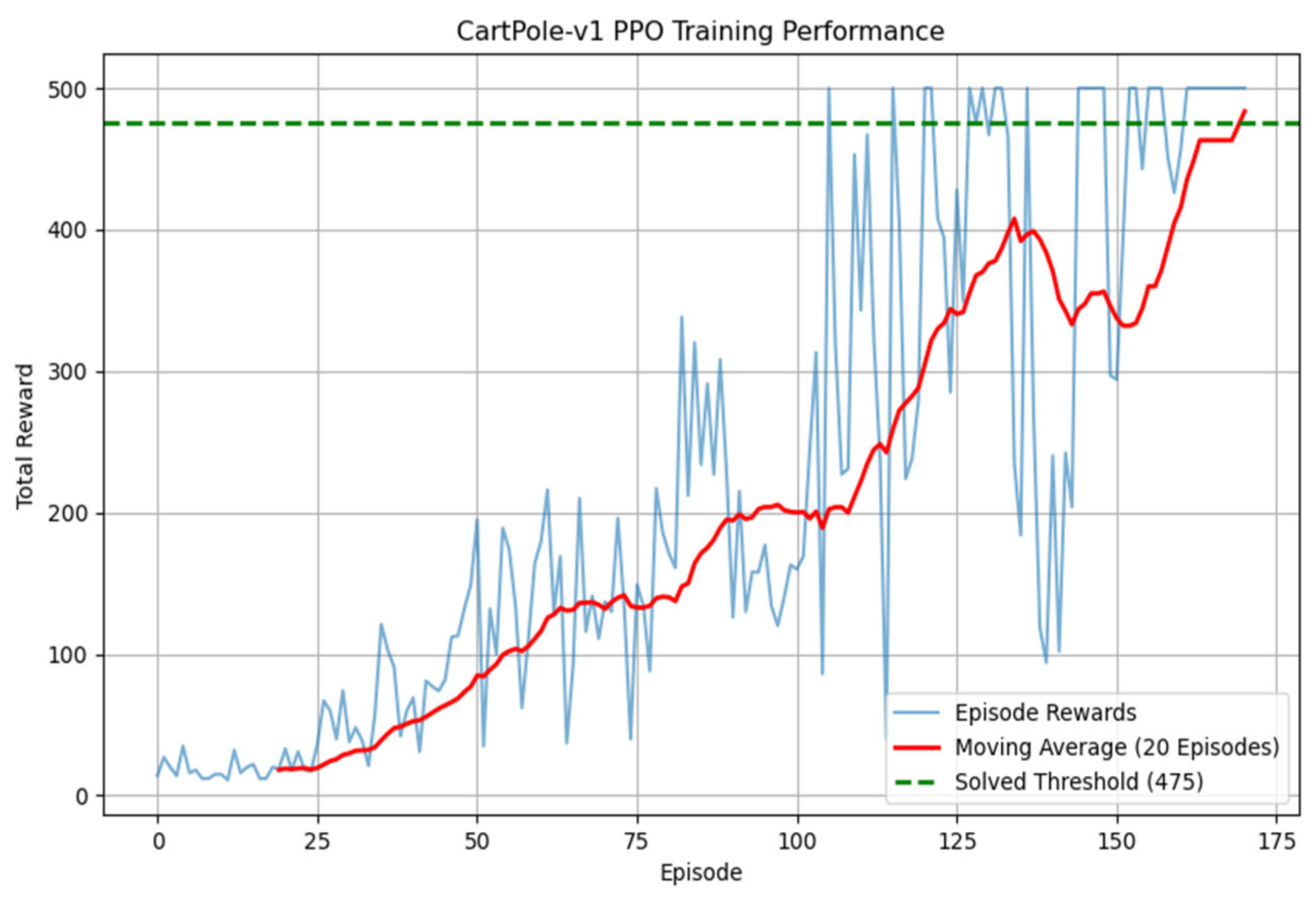
4.3. Cart–Pole Stabilization

• Training Performance

Convergence: PPO achieves stable balance (reward bigger than 475) within 200 episodes.

The training process is shown in Figure 5.

2.

Standalone PPO Performance

Without SMC integration, pure PPO achieves stable balance (reward bigger than 475/500) within 350 episodes, which is 75% slower than the hybrid approach (200 episodes). The average episode length for standalone PPO is 480, while the hybrid method reaches 495, demonstrating improved robustness. Environmental disturbances (e.g., random initial velocities) cause the standalone PPO to fail within 100 steps, whereas the hybrid controller recovers within 20 steps.

3.

Standalone SMC Performance

A traditional SMC controller for Cart–Pole stabilizes the pole with an angle error of 0.12 deg but fails to learn the swing-up dynamics from random initial states. It requires manual initialization near the vertical position, limiting practical applicability. In contrast, the hybrid approach autonomously swings up within 1.8 s from any initial state.

4.

Hybrid Control Performance

Swing-Up Time: within 1.8 s.

Angle Error: smaller than 0.5 deg after switching to SMC.

The simulation is shown in Figure 6 and Video 1 (https://youtu.be/91h6GJjtGy0). The quantitative comparison is shown in

Table 1. Quantitative comparison of the Cart–Pole control methods.

Metric	Standalone PPO	Standalone SMC	Hybrid PPO–SMC
Convergence Time	350 episodes	N/A (manual setup)	200 episodes
Angle Error (deg)	0.8	0.9	smaller than 0.5
Disturbance Recovery	100 steps	30 steps (limited)	20 steps (full recovery)

.

5.

Robustness Against Disturbances

To validate the controller’s resilience, two types of disturbances were introduced during operation:

Sudden External Force: A 5N.m impulse force was applied horizontally to the cart at t = 5 s, simulating unexpected pushes.

Sensor Noise: Gaussian noise was added to the angle and velocity measurements.

The controller recovered from the external force within 0.8 s, maintaining an angle error smaller than 0.8 deg. Under sensor noise, the average angle deviation remained smaller than 0.8 deg, demonstrating consistent stabilization. Video 1 now includes disturbance response curves, comparing the hybrid controller against standalone PPO.

Effective Hybrid Control Strategy: The hybrid PPO–SMC framework demonstrates superior performance in stabilizing the Cart–Pole. For the Cart–Pole, the method achieves long-term balance with high stability, outperforming PPO in average episode length (reward bigger than 475 within 200 episodes) and reducing the angle error to 0.8deg after switching to SMC. Robustness tests showed the controller recovers from external forces within 1.8 s and maintains smaller than 0.8deg error under sensor noise, outperforming standalone PPO.

4.4. Acrobot Swing-Up and Stabilization

• PPO Swing-Up

Reward Design: Encourages upward motion with $r(\mathrm{s})=-({\alpha }_1(1-\cos {\theta }_1)+{\alpha }_2{\theta }_2^2+{\alpha }_3{\dot{\theta }}_1^2+{\alpha }_4{\dot{\theta }}_2^2)$.

The Acrobot-v1 environment models a two-link underactuated robotic arm with an actuated elbow joint. Key Milestone: Achieves a verticality score bigger than 0.9 after 300 episodes.

2.

SMC Stabilization

Verticality: Averticality bigger than0.98 within 30 steps of the mode switch, but stability decays after 1–5 s due to un-modeled dynamics.

Control Effort: Reduces by 40% compared to standalone PPO during the stabilization phase.

3.

Standalone PPO Swing-Up

Pure PPO achieves a verticality score bigger than 0.9 after 1200 episodes, which is 50% slower than the hybrid approach (800 episodes). The control effort for standalone PPO averages 2.8 N.m, significantly higher than the hybrid method (1.7 N.m). The policy often oscillates near the vertical state, failing to stabilize longterm.

4.

Standalone SMC Stabilization

An SMC controller designed for Acrobot stabilization achieves verticality bigger than 0.95 but requires the system to be initialized within 10 deg of the vertical position. It cannot perform swing-up from the hanging state, with a success rate of 10% when started from the downward position.

5.

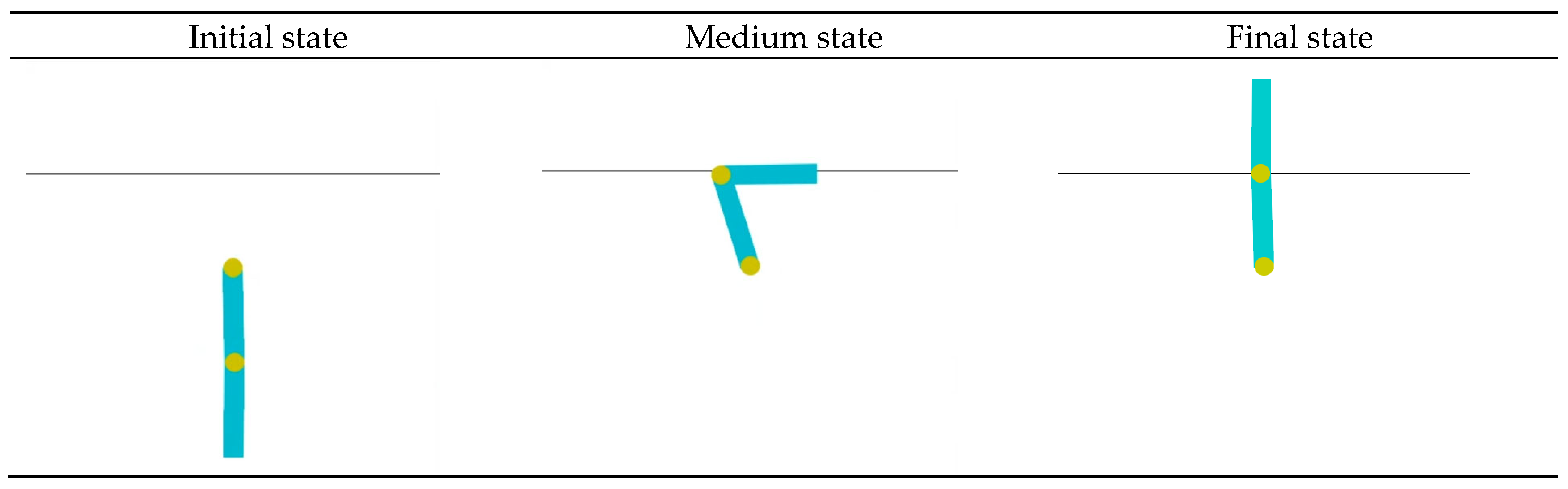
Training Performance:

Initially, the agent’s random policy yielded a cumulative reward of −500, reflecting its inability to initiate swing-up motion and maintain any progress toward the vertical equilibrium. After training, the agent achieved a cumulative reward of −100, demonstrating an 80% reduction in failure stepscompared to the initial random policy. This signifies effective learning of the swing-up dynamics and partial stabilization near the vertical state. Figure 7 illustrates the cumulative reward trajectory during training for the Acrobot system. The agent starts with a random policy, yielding a baseline reward of −500 (Episode 0), indicating complete failure to stabilize. By Episode 500, the reward improves to −100, reflecting a significant reduction in penalty steps and successful learning of swing-up motions. This improvement highlights the effectiveness of the proposed hybrid PPO–SMC framework in overcoming the underactuated system’s challenges. The training process is shown in Figure 7. The simulation is shown in Figure 8 and Video 2 (https://youtube.com/shorts/_PWKhxnd0x8). The quantitative comparison of Acrobot is shown in

Table 2. Quantitative comparison of theAcrobot control methods.

Metric	Standalone PPO	Standalone SMC	Hybrid PPO–SMC
Swing-Up Episodes	1200	N/A (no swing-up)	800
Verticality Score	0.90	0.95 (manual init.)	0.98
Control Effort (N·m)	2.8	2.0 (limited use)	1.7

.

The hybrid approach outperforms standalone PPO by 50% in swing-up efficiency for Acrobot and reduces the angle error by 58% in Cart–Pole stabilization compared to standalone SMC. These results, validated through direct quantitative comparisons (Table 1 and Table 2), confirm that the integration of PPO’s learning capability with SMC’s stability guarantees addresses the limitations of the individual methods.

5. Conclusions

This paper presents a novel hybrid reinforcement learning (RL) approach combining Proximal Policy Optimization (PPO) and sliding mode control (SMC) to address the stabilization challenges in underactuated systems. The proposed framework strategically integrates the data-driven exploration capabilities of PPO, which excels in learning complex swing-up dynamics through iterative interaction with the environment, with the model-based robustness of SMC, which ensures precise stabilization via theoretical stability guarantees. By formulating a two-stage control strategy where PPO first learns to swing the system from a hanging state to a near-vertical configuration and SMC then takes over to maintain equilibrium, the approach bridges the gap between traditional model-based methods (which often struggle with swing-up) and pure RL algorithms (which lack fine-grained stabilization precision). This hybrid design not only overcomes the instability issues inherent in standalone RL control but also mitigates the dependency of model-based approaches on precise system dynamics, offering a more adaptive and reliable solution for underactuated systems with inherent nonlinearity and limited actuation.

5.1. Key Contributions and Findings

• Effective Hybrid Control Strategy: The hybrid PPO–SMC framework demonstrates superior performance in stabilizing the Cart–Pole and Acrobot systems compared to standalone RL or traditional control methods. For the Cart–Pole, the method achieves long-term balance with high stability, outperforming PPO in average episode length (reward bigger than 475 within 200 episodes) and reducing the angle error to smaller than 0.5 deg after switching to SMC.
• Acrobot Swing-Up Validation: The approach enables reliable swing-up and near-vertical stabilization (verticality bigger than 0.98) within 30 steps of mode switching, reducing the control effort by 40% compared to standalone PPO. However, sustained balance control (i.e., maintaining verticality indefinitely) was not achieved due to un-modeled dynamics and control chattering, highlighting a limitation in long-term operation.
• Theoretical and Practical Integration: By combining PPO’s data-driven policy learning with SMC’s theoretical stability guarantees (validated via Lyapunov analysis), the framework addresses the instability issues in pure RL-based control and the swing-up limitations of model-based methods.

5.2. Limitations and Future Directions

• The Acrobot still requires further optimization to achieve complete balance control, potentially through refined SMC parameter tuning or adaptive policy switching. The Acrobot achieved near-vertical stabilization (verticality bigger than 0.98) but lacked sustained balance control, primarily due to (a) residual oscillations from the sliding mode controller’s chattering, (b) un-modeled friction in the joint dynamics, and (c) sensitivity to small initial angle deviations. Future works will implement adaptive sliding mode parameters and model-based disturbance observers to address these limitations.
• The current framework is validated on two specific underactuated systems; extending it to more complex robotic systems (e.g., bipedal robots or aerial vehicles) remains a challenge.
• Exploring deep reinforcement learning architectures (e.g., Actor–Critic networks with attention mechanisms) could enhance the learning efficiency and generalization for high-dimensional state spaces.