Addressing Local Minima in Path Planning for Drones with Reinforcement Learning-Based Vortex Artificial Potential Fields

Abstract

In complex environments, autonomous navigation for quadrotor drones presents challenges in terms of obstacle avoidance and path planning. Traditional artificial potential field (APF) methods are plagued by issues such as getting stuck in local minima and inadequate handling of dynamic obstacles. This paper introduces a layered obstacle avoidance structure that merges vortex artificial potential (VAPF) fields with reinforcement learning (RL) for motion control. This approach dynamically adjusts the target position through VAPF, strategically guiding the drone to avoid obstacles indirectly. Additionally, it employs the Twin Delayed Deep Deterministic Policy Gradient (TD3) algorithm to facilitate the training of the motion controller. Simulation experiments demonstrate that the incorporation of the VAPF effectively mitigates the issue of local minima and significantly enhances the success rate of drone navigation, reduces the average arrival time and the number of sharp turns, and results in smoother paths. This solution harmoniously combines the flexibility of VAPF methods with the precision of RL for motion control, offering an effective strategy for autonomous navigation of quadrotor drones in complex environments.

1. Introduction

In the context of the rapid development of drone technology, quadcopter drones, with their stable structural advantages and flexible control performance, have been widely used in various fields such as aerial photography, surveying, and search and rescue [1,2,3]. However, achieving autonomous navigation for drones in complex environments remains a significant challenge [4,5], with obstacle avoidance and path planning being particularly prominent issues [6,7,8,9,10]. Traditional APF methods, as classic solutions to these problems, guide drone movement by constructing attraction and repulsion force fields, providing an intuitive physical model for path planning. However, this method has notable drawbacks, especially when dealing with local minima and dynamic obstacles, which often lead drones to become trapped in local minimum values, severely limiting their application in complex scenarios [11,12].

At the same time, RL algorithms have demonstrated tremendous potential in the field of drone control [13,14]. By learning through interaction with the environment and autonomously optimizing control strategies, they offer new insights into solving complex dynamic decision-making problems. However, the integration of reinforcement learning with artificial potential fields is still in the exploratory stage. 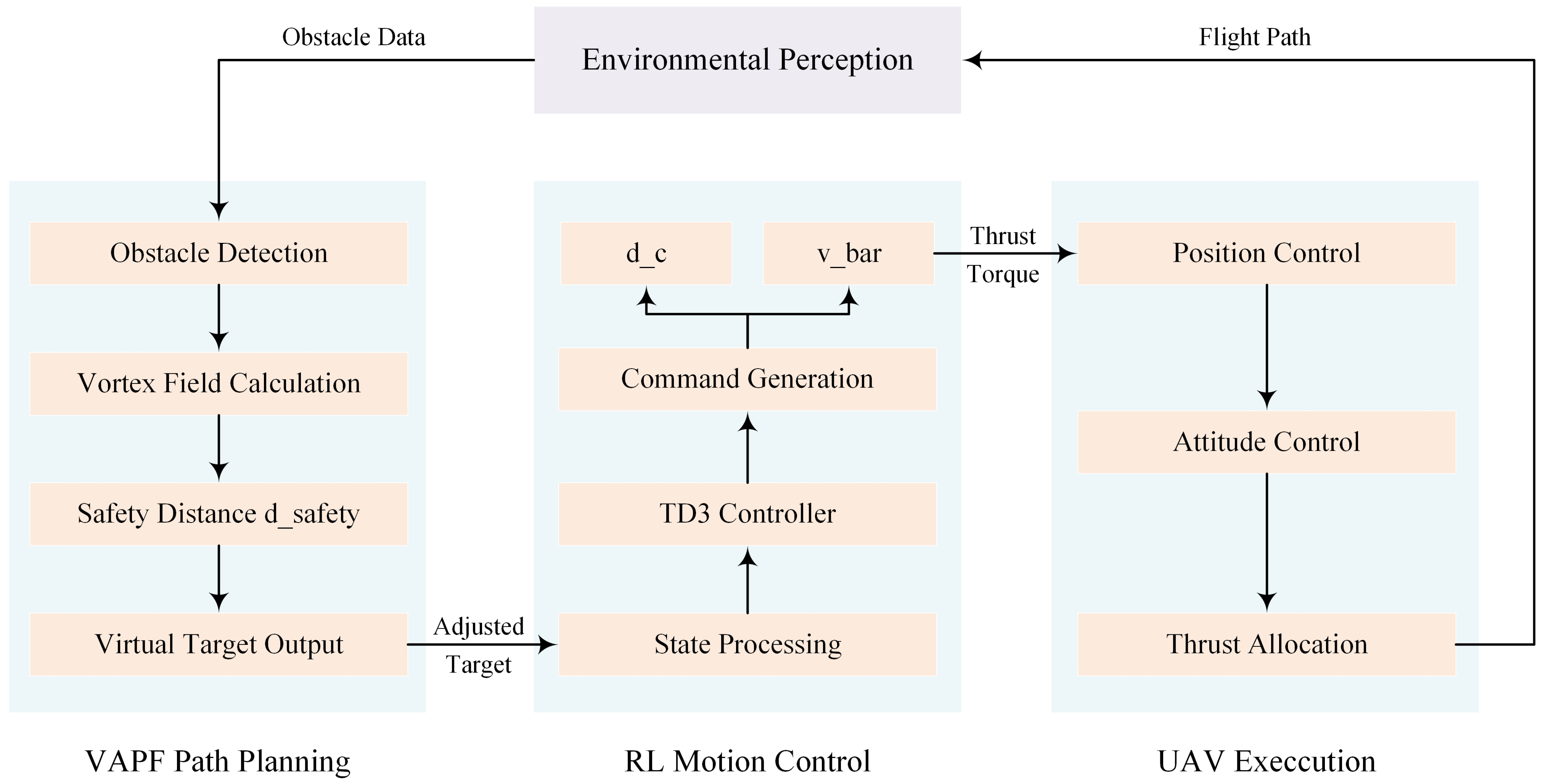Combining the strengths of both to form an efficient autonomous navigation solution has become a focal point and challenge in current research [15]. While existing RL methods for drone control demonstrate proficiency in motion optimization, they often suffer from three key limitations: (1) direct application of potential field forces to drone dynamics can induce oscillatory behavior; (2) inadequate mechanisms to escape local minima inherent in conventional APFs; and (3) limited synergy where RL and potential fields operate in loosely coupled layers rather than a unified framework. In contrast, this study introduces a fundamentally distinct approach: a layered architecture where a VAPF dynamically adjusts the target position input to a TD3-based motion controller. This design decouples obstacle avoidance from direct force application, leveraging the VAPF’s tangential forces to disrupt force symmetries causing local minima, while the RL controller executes precise trajectory tracking toward the adjusted target. This indirect guidance strategy, combined with the VAPF’s inherent stability properties, represents a significant departure from prior RL-APF integrations.

Since its introduction by Khatib in 1986 [16], the APF method has remained a significant research direction in the field of mobile robotics and drone path planning. This method constructs a virtual potential field through mathematical modeling, allowing drones to complete obstacle avoidance and navigation tasks under the influence of potential field forces. However, its inherent problem of local minima has not been thoroughly resolved. When a drone is in an environment with symmetrical obstacles or when a specific geometric relationship forms between the target point and the obstacles, local minima with a zero net force can cause the drone to become stagnant.

To address this issue, scholars have proposed numerous improvement schemes. For instance, Guldner and others suggested using planar harmonic artificial potential fields to achieve robot obstacle avoidance in n-dimensional space, enhancing the smoothness of the potential field by introducing harmonic functions [17]. Domestic scholars Keyu L and others proposed a dynamic obstacle avoidance path planning method for drones based on an improved APF, enhancing the obstacle avoidance effect by adjusting the parameters of the potential field function [18]. However, most of these methods are still limited to static or simple dynamic environments, and their adaptability in complex scenarios is limited.

In recent years, the application of RL algorithms in the field of drone control has become increasingly widespread [19]. The emergence of advanced algorithms such as TD3 has provided powerful tools for high-precision motion control [20]. Park and others have combined dynamic motion primitives with potential fields to achieve motion reproduction and obstacle avoidance through RL [21]. Phang and Hirata have proposed a shared autonomous control method combining human electroencephalography with TD3, demonstrating the potential of RL in human–robot collaboration [22].

However, purely RL methods often face challenges such as low training efficiency and difficult convergence when dealing with large-scale state spaces and complex constraints [23]. To integrate the advantages of APF with RL, some scholars have begun to explore combining the two. Han and others have accelerated formation control based on the Hessian matrix of the APF, providing new insights for the combination of potential fields and optimization algorithms [24]. Rong and others have proposed an autonomous obstacle avoidance decision-making method for MASSs based on the GMA-TD3 algorithm, attempting to integrate RL with the concept of potential fields [25]. However, most of these studies are still in the preliminary stages and have not yet formed a systematic solution.

This study aims to break through the limitations of traditional methods of APF and construct an efficient autonomous navigation solution for drones. The specific objectives include

• Proposing an obstacle avoidance strategy based on VAPF to address the local minima issue of traditional APF methods.
• Integrating RL algorithms to achieve precise control of drone movement.
• Validating the effectiveness of the proposed method through simulation experiments, providing theoretical support for practical applications.

This study adopts a technical route of theoretical modeling, algorithm design, and simulation verification. Firstly, based on the vortex principle in fluid mechanics, a mathematical model of VAPF suitable for drone obstacle avoidance is constructed, and its stability and obstacle avoidance mechanism are analyzed. Secondly, a RL motion controller is designed in combination with the TD3 algorithm, achieving precise control of the drone through a layered control strategy. Finally, simulation experiments are conducted in various complex environments to compare and analyze the performance indicators of different methods, verifying the superiority of the proposed scheme.

The innovations of this study are as follows:

• Deep Integration of VAPF and RL: A novel layered obstacle avoidance structure is proposed, which organically combines VAPF with RL for motion control. This approach retains the intuitive physical model of APF while endowing the system with the ability to learn and optimize autonomously.
• Dynamic Target Adjustment Mechanism: The target position is dynamically adjusted through vortex repulsive forces, enabling the drone to indirectly avoid obstacles. This approach overcomes the limitations of traditional methods where the force field acts directly on the drone.
• Efficient Solution to Local Minima: The introduction of the vortex potential field fundamentally disrupts the symmetric conditions of traditional APF methods. By leveraging tangential forces, the drone is guided out of local minima, significantly enhancing the success rate of path planning.

The results of this study can be widely applied in complex scenarios such as drone logistics delivery, post-disaster rescue, and environmental monitoring. In logistics delivery, it enables efficient obstacle avoidance and path planning for drones in urban building complexes; in post-disaster rescue, it helps drones quickly locate targets in complex environments like ruins; and in environmental monitoring, it ensures that drones can complete monitoring tasks under complex terrain and meteorological conditions. Additionally, this method can provide technical support for collaborative operations of multiple drones, offering broad prospects for engineering applications.

The detailed block diagrams are illustrated in the Figure 1.

The structure of this paper is as follows: Section 2 introduces the drone dynamics model and potential field design; Section 3 details the TD3 algorithm and the layered control architecture; Section 4 presents the experimental results; Section 5 concludes the paper and outlines future directions.

Figure 1. Block diagrams.

Figure 1. Block diagrams.

2. Preliminaries

2.1. Drone Dynamics

Suppose there exist two drones, $w_1$ and $w_2$, moving in a plane with fixed linear velocities. The Euclidean distance between $w_1$ and $w_2$ can be calculated as

$$\mathrm{\Delta }{x}_1=\mathrm{\Delta }{x}_2=\sqrt{{(x_1-x_2)}^2+{(y_1-y_2)}^2},$$

(1)

The line of sight angle $\sigma$ refers to the angle between the drone’s current position and the X-axis of the spatial coordinate system.

$${\sigma }_1=arctan\left({\displaystyle \frac{y_2-y_1}{x_2-x_1}}\right).$$

(2)

2.1.1. Definition of Rotation Matrix

In the dynamic analysis of quadrotor drones, since the thrust f and other related forces acting on the drone are usually defined in the body coordinate system $\left\{x_b,y_b,z_b\right\}$, we need to use a rotation matrix R to transform these forces into the spatial coordinate system $\left\{x_e,y_e,z_e\right\}$. This transformation is performed according to the rotation sequence of the body coordinate system $z_b-y_b-x_b$ to ensure that the direction and magnitude of the forces are correctly represented in the spatial coordinate system.

$$\begin{array}{cc}\hfill R& =R\left(\psi \right)R\left(\theta \right)R\left(\varphi \right)\hfill \\ \hfill & =\left[\begin{array}{ccc}cos\theta cos\psi & cos\psi sin\theta sin\varphi -sin\psi cos\varphi & cos\psi sin\theta cos\varphi +sin\psi sin\varphi \\ cos\theta sin\psi & sin\psi sin\theta sin\varphi +cos\psi cos\varphi & sin\psi sin\theta cos\varphi -cos\psi sin\varphi \\ -sin\theta & sin\varphi sin\theta & cos\varphi cos\theta \end{array}\right].\hfill \end{array}$$

(3)

As shown in the Figure 2, these are the attitude angles of the quadrotor drone. The orientation of an object in a three-dimensional space can be described using Euler angles $\mathrm{\Theta }={|\psi ,\theta ,\phi |}^T$. These angles consist of the roll angle $\psi$, which represents rotation around the front-to-back axis, the pitch angle $\theta$, indicating rotation around the side-to-side axis, and the yaw angle $\phi$, which is the rotation around the vertical axis.

2.1.2. Position Kinematics

$P_e$ represents the position coordinates of the drone, and $V_e$ represents its velocity. Based on the acceleration data obtained from the dynamics output, the current position of the drone can be calculated by applying double integration using the (4).

$$\dot{P_e}=V_e,$$

(4)

$$\begin{array}{c}{F}_{x_1}={\ddot{x}}_1=-V_{e}sin\left({\delta }_1\right){\dot{\delta }}_1,\\ F_{y_1}={\ddot{y}}_1=-V_{e}cos\left({\delta }_1\right){\dot{\delta }}_1.\end{array}$$

(5)

According to the Formula (5), the velocity of the drone is decomposed into radial and tangential components, providing a dynamic foundation for subsequent collision prediction and path planning.

$$\begin{array}{c}{\dot{\mathrm{\Delta }x}}_1=V_{e_1}^{\rho }=V_{e}cos({\delta }_2-{\sigma }_1)-V_{e}cos({\sigma }_2-{\delta }_1),\\ \mathrm{\Delta }{x}_1{\dot{\sigma }}_1=V_{e_1}^{\theta }=V_{e}sin({\delta }_2-{\sigma }_1)+V_{e}sin({\sigma }_2-{\delta }_1).\end{array}$$

(6)

Relative acceleration in the polar coordinate system

$$\begin{array}{c}\dot{V_{e_1}^{\rho }}={\displaystyle \frac{V_{e_1}^{\rho }}{\mathrm{\Delta }{x}_1}}+cos\left({\sigma }_1\right)(F_{x_1}-F_{x_2})+sin\left({\sigma }_1\right)(F_{y_2}-F_{y_1}),\\ \dot{V_{e_1}^{\theta }}={\displaystyle \frac{V_{e_1}^{\rho }{V}_{e_1}^{\theta }}{\mathrm{\Delta }{x}_1}}+cos\left({\sigma }_1\right)(F_{y_1}-F_{y_2})-sin\left({\sigma }_1\right)(F_{x_2}-F_{x_1}).\end{array}$$

(7)

A force analysis is conducted on the drones. To simplify the complexity of the problem and highlight the main forces involved, this paper considers only the thrust generated by the propellers and the gravitational force acting on the drone itself.

$$f=R{f}_b,$$

(8)

$$m\dot{V_e}=f-mg,$$

(9)

Expand to get

$$\left[\begin{array}{c}{\dot{V}}_{X_e}\\ {\dot{V}}_{Y_e}\\ {\dot{V}}_{Z_e}\end{array}\right]={\displaystyle \frac{f_b}{m}}\left[\begin{array}{c}cos\psi sin\theta cos\varphi +sin\psi sin\varphi \\ sin\psi sin\theta cos\varphi -cos\psi sin\theta \\ cos\varphi cos\theta \end{array}\right]-\left[\begin{array}{c}0\\ 0\\ g\end{array}\right],$$

(10)

During the motion, the thrust generated by the drone’s propellers produces torques about the three axes of the body coordinate system, and gyroscopic torque is also present. Therefore, the equations of attitude dynamics are as follows:

$$\tau +G_a=J{\dot{w}}^b+w^b\times J{w}^b.$$

(11)

To simplify the analysis and facilitate the control of the drone, $G_a$ and $w^b\times J{w}^b$ are omitted. Expand to get

$$\left[\begin{array}{c}{f}_x\\ {\tau }_x\\ {\tau }_y\\ {\tau }_z\end{array}\right]=\left[\begin{array}{cccc}-{\displaystyle \frac{\sqrt{2}L}{2}}{d}_{C_T}& -{\displaystyle \frac{\sqrt{2}L}{2}}{d}_{C_T}& -{\displaystyle \frac{\sqrt{2}L}{2}}{d}_{C_T}& -{\displaystyle \frac{\sqrt{2}L}{2}}{d}_{C_T}\\ {\displaystyle \frac{C_T}{2}}& {\displaystyle \frac{C_T}{2}}& {\displaystyle \frac{C_T}{2}}& {\displaystyle \frac{C_T}{2}}\\ {\displaystyle \frac{C_M}{2}}& -{\displaystyle \frac{C_M}{2}}& {\displaystyle \frac{C_M}{2}}& -{\displaystyle \frac{C_M}{2}}\\ {\displaystyle \frac{C_M}{2}}& {\displaystyle \frac{C_M}{2}}& -{\displaystyle \frac{C_M}{2}}& -{\displaystyle \frac{C_M}{2}}\end{array}\right]\left[\begin{array}{c}{\overline{w}}_1^2\\ {\overline{w}}_2^2\\ {\overline{w}}_3^2\\ {\overline{w}}_4^2\end{array}\right],$$

(12)

Among them, L denotes the arm length, $C_T$ and $C_M$ represent the thrust coefficient and torque coefficient, respectively.

In the actual control of quadcopter drones, the implementation of flight maneuvers mainly relies on precise control of the four motor throttles. Various maneuvering actions of the drone, such as roll, pitch, and yaw, are achieved by controlling the rotational speed of each motor. However, the four motor throttles are controlled by pulse-width modulation (PWM) signals u.

$$T_m\dot{\overline{w}}=k_{m}u+b_m-\overline{w}.$$

(13)

This paper employs the SE(3) control framework, which discards the transformation matrix W between Euler angles and angular velocities, thereby avoiding the singularity problem that occurs when the pitch angle approaches. Traditional Euler angle transformation methods are effective in small-angle scenarios; however, they exhibit certain limitations in large-angle situations, such as aggressive drone maneuvers. In contrast, SE(3) directly describes rigid body motion (both rotation and translation), making it applicable even in large-angle scenarios. The hat map is defined as [26].

$$\widehat{e}=\left[\begin{array}{ccc}0& -e_3& e_2\\ e_3& 0& -e_1\\ -e_2& e_1& 0\end{array}\right],$$

(14)

where $\alpha ={[{\alpha }_1,{\alpha }_2,{\alpha }_3]}^{\top }$ is a unit vector. This process transforms three-dimensional unit vectors into antisymmetric matrices, establishing the mathematical link between angular velocity $\omega$ and rotation matrices R.

$$\dot{R}=R\widehat{\omega }.$$

(15)

2.2. Artificial Potential Field

2.2.1. Artificial Potential Field Function

The attractive potential field is used to draw the drone towards the target location. Given a stationary target with coordinates $\left(x,y\right)$ and a drone at its current position $\left(x_i,y_i\right)$, the function describing the attractive potential field is established.As shown in the Figure 3, this depicts the relative position of the quadrotor drone.

$$U_{Att}=\gamma \sqrt{{(x_i-x)}^2+{(y_i-y)}^2},$$

(16)

where $\gamma$ denotes the coefficient of the attractive potential field.

By analyzing the attractive potential energy function, it can be observed that the potential energy decreases as the drone approaches the target. Under the influence of the attractive potential field, the drone $w_i$ moves along the negative gradient direction. The attractive force acting on the drone at its current position can be calculated accordingly.

$$\begin{array}{c}{F}_{x_{i}Att}={\displaystyle \frac{-\partial U_{Att}}{\partial (x_i-x)}}=\gamma cos\left(\sigma \right)=+\gamma {\displaystyle \frac{x-x_i}{r_i}},\\ F_{y_{i}Att}={\displaystyle \frac{-\partial U_{Att}}{\partial (y_i-y)}}=\gamma sin\left(\sigma \right)=+\gamma {\displaystyle \frac{y-y_i}{r_i}},\end{array}$$

(17)

The distance between the drone and the target point is denoted as $r_i$. As shown in the Figure 4 the velocity of the drone is constrained to lie inside a circular region centered on the origin with radius $V_e$.

Substituting into the formula, we obtain

$$\begin{array}{c}{V}_{e_i}^{\rho }=-V_{e}cos(\delta -\sigma ),\\ V_{e_i}^{\theta }=-V_{e}sin(\delta -\sigma ),\end{array}$$

(18)

The drone will fly towards the obstacle, and a collision is imminent, only if two conditions are met: the drone’s relative radial velocity to the obstacle is negative (indicating it is moving closer to the obstacle), and the relative tangential velocity is zero. According to the above equations, when $V_{e_i}^{\theta }=0$, $V_{e_i}^{\rho }=-V_{e_i}$.

To simplify the proof process, we define $\widetilde{V_{e_i}^{\rho }}=V_{e_i}^{\rho }+V_{e_i}$.

2.2.2. Vortex Artificial Potential Field Function

VAPF is an innovative improvement based on the APF method. The core idea of VAPF is to regard the target point as a vortex source, which generates a vortex field around the target point. Under the action of the vortex field, the drone moves towards the target point along the path of the vortex field, thus avoiding falling into local minima. The potential function of VAPF usually consists of two parts: attractive potential and repulsive potential. The attractive potential is generated by the vortex field of the target point, while the repulsive potential is generated by obstacles, and this paper only considers dynamic vortex repulsive potential.

The repulsive function for the vortex repulsion field is defined as

$$U_{Repi}=\left\{\begin{array}{cc}\epsilon (cos{\chi }_1){\displaystyle \frac{|{\overline{V}}_{i,j}|}{\mathrm{\Delta }{\chi }_1}},\hfill & {\displaystyle \frac{\pi }{2}}<{\chi }_1<\pi \hfill \\ 0,\hfill & \mathrm{otherwise}\hfill \end{array}\right.,$$

(19)

The potential function of the VAPF is continuous and differentiable within its domain, ensuring the stability of path planning. The VAPF is isotropic, meaning that the value of the potential function depends only on the distance between the robot and the target or obstacles, not on the specific position or orientation of the drones.

Assume there are two drones, $w_i$ and $w_j$, and they are on a collision course; that is, at this moment, the relative radial velocity between the two drones is less than zero, and the relative tangential velocity is zero. Based on the analysis of the above equations, it can be seen that when the two drones are on a collision path, the repulsive potential field is activated, and at this time $cos\left({\chi }_1\right)<0$, with ${\chi }_1$ falling within a certain range $({\displaystyle \frac{\pi }{2}},\pi ]$. The schematic diagram of the decomposition of the vortex repulsive force exerted on the quadrotor drone is shown in Figure 5.

Under the influence of the repulsive potential field, the drone moves in the direction of the steepest descent of the repulsive potential energy; that is

$${\displaystyle \frac{\partial U_{Re{p}_i}}{\partial (x_{R_j}-x_{R_i})}}=-{\displaystyle \frac{\lambda V_e^{\rho }}{V_{rel}{r}^2}}(2V_e^{\theta }sin{\theta }_i+V_e^{\rho }cos{\theta }_i),$$

(20)

$${\displaystyle \frac{\partial U_{Re{p}_i}}{\partial (y_{R_j}-y_{R_i})}}=+{\displaystyle \frac{\lambda V_e^{\rho }}{V_{rel}{r}^2}}(2V_e^{\theta }cos{\theta }_i-V_e^{\rho }sin{\theta }_i).$$

(21)

To reflect the characteristics of the VAPF, the direction of the repulsive vortex field is fixed, and the control input of the drone is designed in the following form:

$$\begin{array}{c}{F}_{x_i,Rep}=-{\displaystyle \frac{\partial U_{Re{p}_i}}{\partial (x_{R_j}-x_{R_i})}},\\ F_{y_i,Rep}=+{\displaystyle \frac{\partial U_{Re{p}_i}}{\partial (y_{R_j}-y_{R_i})}}.\end{array}$$

(22)

2.3. Twin Delayed Deep Deterministic Policy Gradient

RL algorithms can be described as a Markov Decision Process (MDP), which consists of a state space S, an action space A, state transition probabilities P, an immediate reward function R, and a discount factor k. At each time step, the agent receives the current state and selects an action based on its policy. The environment transitions to the next state according to the state transition probability. At the same time, the agent receives an immediate reward. The goal of the agent is to find an optimal policy that maximizes the expected cumulative reward starting from the initial state.

$$G_t=\sum _{i=t}^{\infty }{k}^{i-t}{r}_i.$$

(23)

This paper adopts the TD3. This algorithm is a model-free-critic deep reinforcement learning algorithm that combines the idea of double Q-learning and deep deterministic policy gradient.The specific algorithm process is shown in Figure 6. Among (27), ${\mu }_{\alpha }$ is the current actors’ network and $Q_{w_i}$ the $i-th$ critics’ network $(i=1,2)$.

It is mainly used for training motion controllers, which adopt two evaluation networks, $Q_{w_1}$ and $Q_{w_2}$, and reduce the overestimation problem of action values. The TD3 algorithm also has the characteristics of smooth regularization and delayed update, which can reduce the changes of target update and ensure the stability of the strategy.

The formula for the target actor’s online update is as follows:

$$a_{t+1}^{\sim }={\mu }_{\alpha }\left(s_{t+1}\right)+\epsilon ,$$

(24)

$$\epsilon \sim clip(N\left(0,\tilde{\sigma }\right),-c,c),$$

(25)

Among them, ${\mu }_{\alpha }$ is the target actor network, $\epsilon$ is the Gaussian noise, $\tilde{\sigma }$ is the standard deviation of the noise, and c is the boundary of the noise.

The loss function of the evaluation network is as follows:

$$L_{TD,3}\left(w_i\right)=E_{s_t,a_t,s_{t+1},\sim D}\left[\left(r_t+kmin{Q}_{w_j}\left(s_{t+1},a_{t+1}\right)-Q_{w_i}\left(s_t,a_t\right)\right]\right.,$$

(26)

Among (26), D is the replay buffer, k is the discount factor, and $a_{t+1}$ is the action of the next state generated based on the target actor network.

The actor network update function is

$${\nabla }_{\mathit{\alpha }}J\left(\mathit{\alpha }\right)=E_{a_t\sim {\mu }_{\alpha }\left({\mathbf{s}}_t\right)}\left[{\nabla }_{\mathit{\alpha }}{\mu }_{\alpha }\left(s_t\right)w_i{Q}_i({\mathbf{s}}_t,{\mathbf{a}}_t)\right],$$

(27)

3. Methods

3.1. Potential Field Stability Proof

3.1.1. Artificial Potential Field Stability Proof

The following uses a Lyapunov function to prove the stability of the potential field. The Lyapunov function is defined as

$$V_{Latt}=\gamma \times r_i+{\displaystyle \frac{1}{2}}{V}_e^{{\theta }^2}+{\displaystyle \frac{1}{2}}\widetilde{V_e^{{\rho }^2}},$$

(28)

Differentiating this formula yields the following:

$$\dot{V_{LAtt}}=-V_e(\gamma -{\displaystyle \frac{V_e^{{\theta }^2}}{r}}),$$

(29)

Assuming a safe distance $r^{*}>0$, when $\gamma >{\displaystyle \frac{V_e^2}{r^{*}}}$ is set, $\dot{V_{LAtt}}$ is less than 0, which indicates that the distance is gradually decreasing, meaning the energy of the entire system $V_{LAtt}$ is gradually decreasing, tending towards stability, until $r=r^{*}$. It can be known that this nonlinear dynamical system will move towards the direction of $r=r^{*}$, and the drone is attracted to the vicinity of the safe distance, forming a safe obstacle avoidance environment. However, there may be special conditions where, at the initial moment $t_0$, the tangential velocity vector of the drone is 0, and the radial velocity vector is $-V_e$, but at this time, the distance between the drone and the target position is not zero. In this case, the drone may stop radial movement at a non-zero distance but move laterally at maximum tangential velocity. This special condition requires further verification.

$$\dot{V_e^{\rho }}=-\alpha \times \gamma ,\left(\alpha <1\right),$$

(30)

Integrate this formula to obtain the drone’s radial velocity.

$$V_e^{\rho }=V_e^{{\rho }_0}-\alpha \gamma t,$$

(31)

Integrating this formula yields the distance between the drone and the target position.

$$r\left(t_1\right)=r_0+{\int }_0^{t_1}{V}_e^{\rho }\left(t\right)dt=r_0+{\displaystyle \frac{(V_e^{{\rho }_0}-V_e)}{2\alpha \gamma }},$$

(32)

When the drone approaches the target position at maximum speed, that is

$$t_1={\displaystyle \frac{V_e^{{\rho }_0}+V_e}{\alpha \gamma }},$$

(33)

Analyzing the Formulas (32) and (33), it can be observed that $r\left(t_1\right)>r_0>r^{*}$. When the drone satisfies the collision condition, at that moment, the distance between the drone and the target point meets the requirement of the safe distance. Within the time range $\left[0,t_1\right)$,$\dot{V_{LAtt}}<0$. At this point, the drone will be trapped between the target positions. When $[t_1,\infty )$, the drone’s trajectory gradually converges to the target point while satisfying the collision condition. The existence of the tangential velocity component $V_e^{\theta }\left(t_1\right)=0$ indicates that, during the initial movement phase, the drone actively moves away from the target to adjust its heading and then approaches the target along a radial path at a constant speed v, ultimately achieving precise proximity.

In summary, at the equilibrium position $(r,V_e^{\theta },V_e^{\rho })=(0,0,0)$, the system reaches a stable state.

3.1.2. Dynamic Vortex Field Stability Proof

The following uses a Lyapunov function to prove the stability of the vortex repulsive potential field. The Lyapunov function is defined as

$$V_{LRep}=\mathrm{\Delta }x+{\displaystyle \frac{1}{2}}{V}_{rel}^{{\theta }^2}+{\displaystyle \frac{1}{2}}{V}_{rel}^{{\rho }^2},$$

(34)

Substituting the formula $V_{rel}^{{\theta }^2}+V_{rel}^{{\rho }^2}=V_{rel}^2$, we obtain:

$$V_{LRep}=\mathrm{\Delta }X+0.5V_{rel}^2,$$

(35)

By analyzing Formula (35), r can be regarded as potential energy and $0.5V_{rel}^2$ as kinetic energy. At this point, the Lyapunov function can be viewed as the sum of the potential energy component and the kinetic energy component.

When the relative radial velocity between the two drones is $V_{rel}^{\rho }=-2V_e<0$ and the relative tangential velocity is, the two drones are on a collision path. When the distance between the two drones $V_{rel}^{\theta }=0$, the collision occurs. At this moment, the Lyapunov function value $V_{LRep}=0$. That is, at the dynamic equilibrium point $V_e^{\rho }=V_e^{\theta }=0$, the Lyapunov function value is zero, and the system is in a stable state.

Assuming that at the initial moment, the distance between the two UAVs is $r_0$. Differentiating the Lyapunov function along the trajectory of the UAVs yields

$$\dot{V_{LRϵp}}=V_{rel}^{\rho }\left(1+{\displaystyle \frac{6\lambda }{V_{rel}{r}^2}}{V}_{rel}^{\rho }{V}_{rel}^{\theta }\right),$$

(36)

When $\dot{V_{LRep}<0}$, it indicates that the system is moving in the direction of decreasing energy, and at this time, the two drones move away from each other, thereby avoiding a collision.

By introducing the VAPF, the system can maintain stability while avoiding collisions and prevent falling into local minima. The equation takes into account the ratio of separation distance, ensuring that the distance between drones does not decrease too rapidly, thus preventing the occurrence of a collision.

$${\displaystyle \frac{{\dot{V}}_{LRep}}{{\dot{V}}_r}}=\left(1+{\displaystyle \frac{6\lambda }{V_{rel}{r}^2}}{V}_{\gamma }{V}_{\theta }\right),$$

(37)

Through Formula (37), the specific collision avoidance process between the two drones can be analyzed. At the initial moment $t_0$, the rotational speed of the drone $\dot{V_{rel}^{\theta }}$ is greater than zero, and the relative radial velocity $V_{rel}^{\rho }$ is less than zero. At this moment, the two drones begin to move away from each other. However, the relative distance between the two drones is decreasing, and the drones are moving closer to each other.

For specific parameters $\lambda$ and initial distance $r_0$, the following holds $t_1$

When $t<t_1$, the separation velocity does not exceed $V_{LRep}$;

When $t=t_1$, $\dot{V_{LRep}=0}$,$V_{LRep}$ reaches its minimum value;

When $t>t_1$, due to the positive value of the lateral repulsive field component, the equilibrium state at the origin gradually becomes unstable.

At the same time, as the relative displacement between the two drones increases, the angular and radial coupling terms in the velocity components $V_{rel}^{\theta }/\mathrm{\Delta }X$ and $-V_{rel}^{\rho }{V}_{rel}^{\theta }/\mathrm{\Delta }X$ significantly affect $\dot{V_{LRep}^{\rho }}$ and $\dot{V_{LRep}^{\theta }}$. When $t=t_2$ (satisfying $t_2>t_1$), the radial velocity approaches zero, while the angular velocity $V_e^{\theta }$ converges to the relative velocity $V_{rel}$. In this state, the motion trajectory in the velocity phase space gradually approaches the steady-state point, causing the collision detection condition to become invalid. Therefore, the drone control system will actively terminate the intervention of the VAPF.

3.2. Hierarchical Obstacle Avoidance Structure

To achieve precise control of drone motion, this paper separates linear motion control from rotational motion control by dividing the control system into two layers: translational control and angular control. The translational control layer consists of horizontal control and vertical control. Translational control is primarily responsible for regulating the drone’s position and velocity, while angular control is dedicated to managing the drone’s attitude [27].

$$\begin{array}{c}{s}^x={\left[e^x,v^x,\mathrm{sign}\left(e^x\right)e^z,\mathrm{sign}\left(e^x\right)v^z,\ddot{\theta },\dot{\theta }\right]}^T,\\ s^y={\left[e^y,v^y,\mathrm{sign}\left(e^y\right)e^z,\mathrm{sign}\left(e^y\right)v^z,\ddot{\varphi },\dot{\varphi }\right]}^T,\\ s^z={\left[e^z,v^z\right]}^T,\\ s^{\xi }={\left[e^{\xi },v^{\xi }\right]}^T.\end{array}$$

(38)

Among Formula (38), $sign\left(e^x\right)e^z$ represents the position error component that adjusts the vertical direction according to the direction of $e^x$.

In actual control, the parameter settings for the horizontal control, vertical control, and angular control of the unmanned aerial vehicle are ${\alpha }_h,{\alpha }_v,{\alpha }_a$. The unit vector of the body coordinate system in the Earth coordinate system is $x_b,y_b,z_b$, where $z_b$ is represented as $z_b^x,z_b^y,z_b^z$.

The Euler angular error is extracted from the rotation matrix using the formula

$$e_R={\left[e^{\varphi },e^{\theta },e^{\phi }\right]}^T={\displaystyle \frac{1}{2}}{\left(R_d^{T}R-R^T{R}_d\right)}^V,$$

(39)

V represents the inverse operation of the hat mapping, $R_d$ represents the expected rotation matrix, and $e^{\xi }$ represents the error value corresponding to the Euler angle, where $\xi =\theta ,\varphi ,\phi$. From Formula (39) for solving the rotation matrix, it can be known that the three parameters of ${\theta }_d$, ${\phi }_d$, and ${\varphi }_d$ are uniquely determined $R_d$. Translation control is carried out on the corresponding $x-axes$, $y-axes$, and $z-axes$, respectively, and the required forces are solved using the following formulas:

$$\begin{array}{c}{f}_d^x=m{a}_t{\mu }_{v_h}\left(s^x\right),\\ f_d^y=m{a}_t{\mu }_{v_h}\left(s^y\right),\\ f_d^z=m\left(a_t{\mu }_{v_h}\left(s^z\right)+g\right),\end{array}$$

(40)

Among Formula (40), $f_d^x$, $f_d^y$, and $f_d^z$ respectively represent $x-axes$, $y-axes$, and $z-axes$. The force required for the axis to perform translation control, $a_t$, represents the maximum translation acceleration that can be provided, and ${\mu }_{v_h}\left(s^x\right)$ represents the control signal in the horizontal direction.

$$\begin{array}{c}{\theta }_d=arctan\left({\displaystyle \frac{c_{{\phi }_d}{f}_d^x+s_{{\phi }_d}{f}_d^y}{f_d^z}}\right),\\ {\varphi }_d=arcsin\left({\displaystyle \frac{s_{{\phi }_d}{f}_d^x-c_{{\phi }_d}{f}_d^y}{∥{\left[f_d^x,f_d^y,f_d^z\right]}^T∥}}\right),\end{array}$$

(41)

According to Formula (41), the expected roll angle ${\varphi }_d$ and pitch angle ${\theta }_d$ can be calculated.

$$f_d={\displaystyle \frac{f_d^z}{c_{\varphi }{c}_{\theta }}},$$

(42)

$${\tau }_d^{\xi }=I^{\xi }{a}_r{\mu }_{v_a}\left(s^{\xi }\right),$$

(43)

$c_r$ represents the maximum angular acceleration that the unmanned aerial vehicle can generate. The desired steady-state rotor speed $\overline{w}=k_{m}u+b_m$ is obtained by solving the inverse matrix of the formula, and finally the PWM signal u is calculated.

Use (44) to set the reward mechanism for the reinforcement learning environment in the angular, vertical, and horizontal directions

$${\tau }_i^{\xi }=|e_t^{\xi }|-|e_{t+1}^{\xi }|,$$

(44)

Among Formula (44), $e_t^{\xi }$ represents the time error value at a moment t. When the error value gradually decreases to 0, the system will give a positive reward; otherwise, the reward will be negative. The significant advantage of this design lies in the fact that no hyperparameters need to be manually adjusted.

3.3. Motion Controller Training

In this study, the templates of the Angle controller and the horizontal controller are pitch and x axis controllers, which means that the values during training $\xi$ are $\theta$, x, and z. Since the variables $s^x$ contain relevant information about the drone’s altitude and pitch angle, their accuracy is directly affected by the performance of the vertical direction and pitch direction controllers. Therefore, the axis controller is trained only after obtaining these two key parameters, $v_a$ and $v_h$; the training process of the motion controller also follows this specific sequence. First, train the rolling and vertical controllers separately.

When training the pitch controller, let

$$f_d={\tau }_{\varphi }^d={\tau }_{\phi }^d=0,$$

(45)

$${\tau }_{\theta }^d=l_0{a}_r{\mu }_{v_h}\left(s^{\theta }\right).$$

(46)

When training the vertical controller, let

$$f_d=m\left(a_t{\mu }_{v_h}\left(s^z\right)+g\right)/c_{\varphi }{c}_{\theta },$$

(47)

$$R_d=0.$$

(48)

3.4. State Transition

3.4.1. Scope Limitation

After training the motion controller using the reinforcement learning algorithm, precise control of the motion state of the unmanned aerial vehicle can be achieved in the corresponding dimension. During the training process, it is impossible to obtain position error data of any size, mainly targeting small-scale offset situations. In the actual operation process, the unmanned aerial vehicle may deviate from the target position by a large margin. At this time, the unmanned aerial vehicle motion control system may lose precise control of the unmanned aerial vehicle. To solve this problem, this paper introduces a shearing mechanism. That is, a position error limit is added in the horizontal direction to avoid the occurrence of large horizontal position errors. In the vertical direction, considering the practical application background, the upper and lower limits of height are added to limit the vertical position error.

3.4.2. Speed Limit

Just like the range limitation, after reinforcement learning training, the motion controller can effectively control the flight speed of drones, which is specifically manifested as follows: when the flight speed of the drone is less than $\tilde{v}$, the acceleration signal of the controller ${\mu }_v\left(s\right)>0$; When the speed of the unmanned aerial vehicle is greater than $\tilde{v}$, ${\mu }_v\left(s\right)<0$; this feature helps to stabilize the system, where $\tilde{v}$ is the maximum speed preset by the motion controller. However, in the actual operation control, the preset maximum speed of the motion controller is relatively large, and there may be a risk of loss of control. To solve this problem, in this paper, the upper limit of the drone speed is manually set to limit the speed of the drone during the test stage and ensure operational safety.

In order to make the training system learn more efficiently, this paper uses $\tilde{v}/\overline{v}$, the original data for scaling, where $\overline{v}$ is the maximum speed set by humans. Using this ratio, the original speed error range $[0,\tilde{v}]$ is mapped to the new range $[0,\overline{v}]$. The conversion can not only make full use of the existing data but also respond quickly in complex environments. While ensuring stability of flight attitude, potential dangers can be avoided.

3.4.3. Isotropy

However, current control strategies cannot guarantee this isotropy. To solve this problem, as shown in Figure 7. in this paper, the control force is decomposed into two dimensions, and the components of the force vector are decomposed radially and tangentially relative to the horizontal error vector $e_h={[e^x,x^y,0]}^T$.

The unit radial vector and tangential vector are defined to rerepresent the direction and magnitude of the force vector, thus achieving isotropic control performance.

$$h={\displaystyle \frac{e_h}{\parallel e_h\parallel }},$$

(49)

$$T\left(h\right)=h\times {\left[0,0,-1\right]}^T,$$

(50)

The horizontal state has been modified to

$$\begin{array}{c}{s}^{\rho }={\left[e^{\rho },{\left(\tilde{v}/\tilde{v}\right)}^{\mathbf{T}}h,\mathrm{sign}\left(e^{\rho }\right)e^z,\mathrm{sign}\left(e^{\rho }\right)v^z,\tilde{\theta },\dot{\tilde{\theta }}\right]}^{\mathsf{T}},\\ s^{\theta }={\left[e^{\theta },{\left(\tilde{v}/\tilde{v}\right)}^{\mathbf{T}}T\left(h\right),\mathrm{sign}\left(e^{\theta }\right)e^z,\mathrm{sign}\left(e^{\theta }\right)v^z,\tilde{\varphi },\dot{\tilde{\varphi }}\right]}^{\mathsf{T}},\end{array}$$

(51)

Among Formula (51), $e^{\rho }$, $e^{\theta }$, $\tilde{\theta }$, and $\tilde{\varphi }$ are respectively defined as

$$\begin{array}{c}{e}^{\rho }=clip\left(e_d^{T}h\right),-d_c,d_c),\\ e^{\phi }=clip({\mathit{e}}_d^{T}T\left(h\right)-d_c,d_c),\end{array}$$

(52)

$$\begin{array}{c}\tilde{\theta }=arctan{\displaystyle \frac{z_b^{T}h}{z_b^z}},\\ \tilde{\varphi }=arctan{\displaystyle \frac{z_b^{T}T\left(h\right)}{z_b^z}},\end{array}$$

(53)

The formula is modified in the following way:

$${[f_x^d,f_y^d,0]}^T=m{a}_t{\mu }_{v_h}\left(s^{\rho }\right)h+m{a}_t{\mu }_{v_h}\left(s^{\theta }\right)T\left(h\right),$$

(54)

So far:

$$e^{\rho }=\sqrt{{\left(e^x\right)}^2+{\left(e^y\right)}^2}\ge 0,$$

(55)

$$e^{\theta }=0.$$

(56)

When it comes to the motion control of quadcopter unmanned aerial vehicles, the reinforcement learning algorithm is applied to achieve precise motion control. In this paper, a hierarchical control structure is adopted. The reinforcement learning algorithm is only used in the low-level motion control aspect and does not participate in the higher-level motion planning. In the process of obstacle avoidance during the movement of drones in this paper, the APF is utilized to dynamically adjust the input of RL control, thereby indirectly influencing the target position of the drones. Realize obstacle avoidance for unmanned aerial vehicles. Similar to the classical potential field method, in this method, obstacles located within the sensing range of drones and on the collision path will generate vortex repulsive forces. However, unlike traditional APF, this repulsive force is not directly applied to the drone but is used to modify the target position. In this way, it can be ensured that the drone can effectively track the target while avoiding obstacles. The specific implementation is accomplished by inputting the adjusted position error signal into the RL motion controller.

$$e^{\rho }=clip(e^{T}h,0,d_c)-F_{rep}^{T}h,$$

(57)

$$e^{\theta }=-F_{rep}^{T}T\left(h\right).$$

(58)

Before the vortex repulsive force adjusts the position error, the control system will first implement distance limitation $d_c$ to prevent the radial position error and tangential position error from being completely restricted during the truncation effect so as to ensure that the vortex repulsive force generated by the obstacles close to the drone plays a major role in the motion adjustment process of the drone. When the distance limit fails, the correction effect of the vortex repulsive force on the target will be greatly reduced; especially when the drone is far from the original target position, the correction effect can almost be ignored.

During the movement of the drone, the distance, angle, and other geometric relationships with the surrounding obstacles change; thus, the vortex repulsive force keeps changing during the movement of the drone. Under the dynamic action of the vortex repulsive force, the position of the target also changes dynamically. Therefore, in the process of motion control, the speed of the drone should not only be considered, but also the speed of the target. Since the training process assumes that the target position remains fixed, to solve this problem, during the training process, the velocity $v^{goal}$ is taken as the derivative of the vortex repulsive force with respect to time. The moving speed of the target.

$$v^{\mathrm{goal}}={\dot{F}}_{\mathrm{rep}}=-\sum _{i,d_i\le d}{\nabla }_{\mathit{P}}^2{U}_{repi}(\parallel e_i\parallel )\dot{P}=-\sum _{i:d_i\le d}{H}_{i}v,$$

(59)

$d_i$ represents the horizontal distance between the drone and the $i-$ th obstacle and represents the Hessian matrix where the $i-$ th obstacle represents the repulsion field.

$${\mathit{v}}^{\mathrm{rad}}=\left\{\begin{array}{cc}{\mathit{v}}_{\mathrm{tar}}\hfill & {\mathit{h}}^T{\mathit{v}}_{\mathrm{tar}}>0\hfill \\ 0\hfill & {\mathit{h}}^T{\mathit{v}}_{\mathrm{tar}}\le 0\hfill \end{array}\right.,$$

(60)

By using Formula (60), it can be ensured that the horizontal position error is limited within the range d. Finally, the horizontal state during the testing phase becomes

$$\begin{array}{c}{s}^{\rho }={\left[e^{\rho },\left(\tilde{v}/\tilde{v}\right){\left(v-v^{\rho }\right)}^{T}h,\mathrm{sign}\left(e^{\rho }\right)e^z,\mathrm{sign}\left(e^{\rho }\right)v^z,\tilde{\theta },\dot{\tilde{\theta }}\right]}^T,\\ s^{\theta }={\left[e^{\theta },\left(\tilde{v}/\tilde{v}\right){\left(v-v^{tar}\right)}^{T}T\left(h\right),\mathrm{sign}\left(e^{\theta }\right)e^z,\mathrm{sign}\left(e^{\theta }\right)v^z,\tilde{\varphi },\dot{\tilde{\varphi }}\right]}^T.\end{array}$$

(61)

This paper proposes an innovative integration scheme of RL motion control and APF obstacle avoidance technology. The core mechanism lies in limiting the adjustment of the state space to the test stage, without the need to modify the internal structure of the trained motion controller. Compared with the traditional way of directly applying artificial potential field forces to drones by the potential field method, this scheme realizes indirect navigation control by dynamically adjusting the coordinates of the virtual target. Essentially, it constructs a dynamic waypoint generation mechanism based on the PF theory. This indirect control strategy has formed waypoint sequences with obstacle avoidance characteristics in practical applications. When successfully applied to the autonomous navigation system of drones, it shows two major advantages: it not only completely retains the decision-making architecture of the pre-trained controller, but also achieves more flexible obstacle avoidance path planning through the mediating role of virtual targets.

4. Results

4.1. Training Parameter Settings

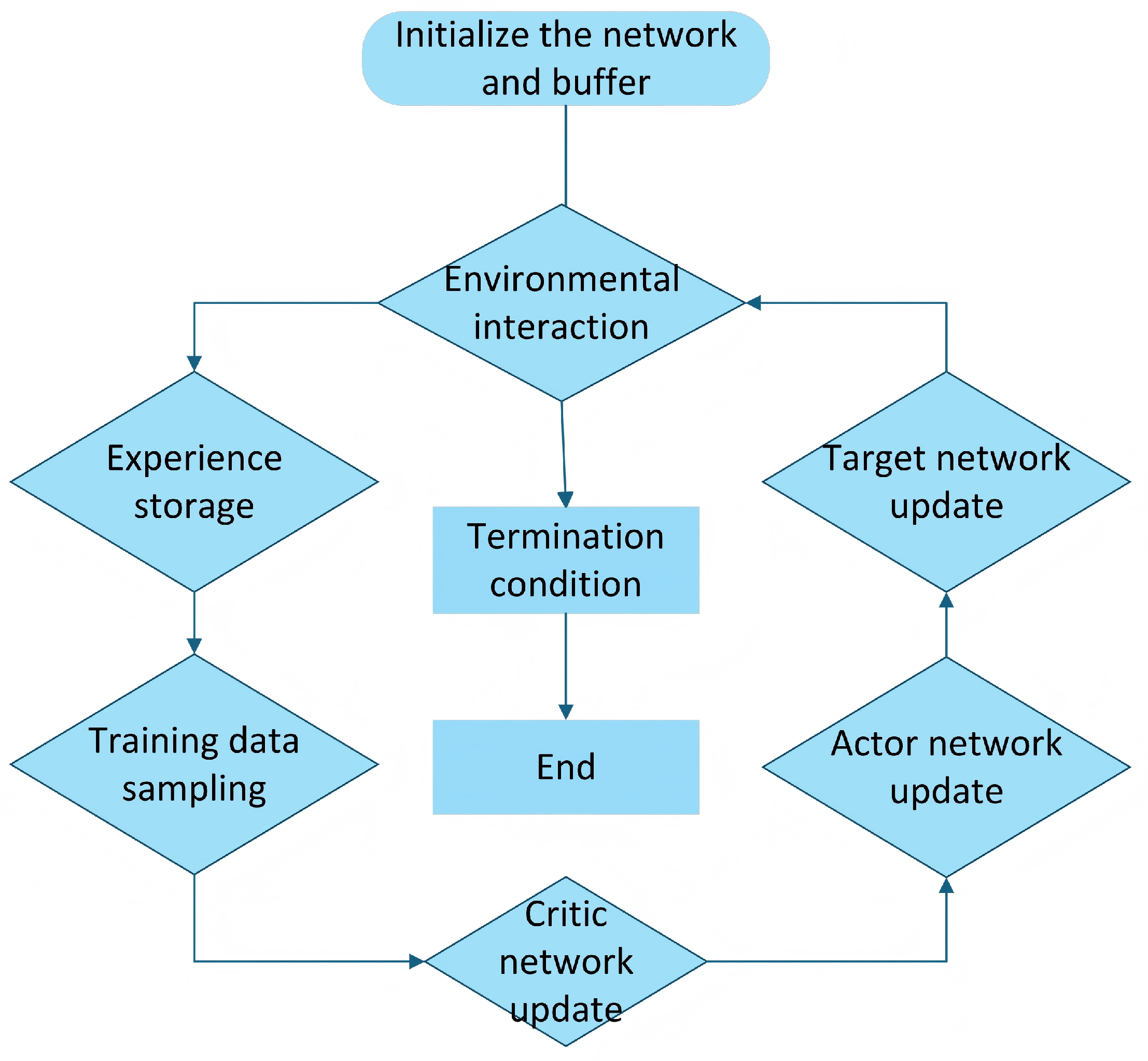
During the training phase, all drones are trained using the TD3 algorithm without considering obstacles and external disturbances. The dynamics of the drones follow the Crazyfile2.0 model. The target neural network is updated every 512 time steps $(C=512)$, with target values randomly selected from a uniform distribution. The angular target values range from $-{\displaystyle \frac{\pi }{2}}$ to ${\displaystyle \frac{\pi }{2}}$, and the translation target values range from −5 to 5. The maximum translation acceleration $C_t$ is limited to 5 m/s², and the maximum angular acceleration $C_r$ is limited to 20 rad/s². The training process involves training two controllers, each consisting of 200 training rounds. The maximum length of each round is set to 500 and 1000. A two-layer MLP is used to build an RL network, with each layer containing 32 nodes. In the TD3 training phase, the discount factor $\gamma$ is set to 0.9, and the capacity of the experience replay buffer $\left|D\right|$ is set to $1\times {10}^4$. Storing a large number of experience samples improves the efficiency and stability of the training process. The batch size N is set to 512, meaning that 512 samples are selected for calculation and model parameter updates in each training iteration. An appropriate batch size enhances training efficiency without significantly increasing memory requirements and computational costs. The network uses the Adam optimizer for updates, which is a common optimization algorithm used to adjust the weights and biases of the neural network to minimize the loss function. The learning rate (v) is set to $1\times {10}^{-4}$. An appropriate learning rate ensures stable updates without causing instability, oscillation, or falling into local optima. The specific parameter settings are as follows.The specific parameter settings are shown in

Table 1. Specific Training Parameter Design.

Symbols	Descriptions	Values
$\left|D\right|$	Relay Buffer Size	$1\times {10}^4$
N	Batch Size	512
$\gamma$	Discount Factor	0.9
k	Target Update Rate	0.1
$\nu$	Learning Rate	$1\times {10}^{-4}$
$ϵ$	Noise Variance	0.2
v	Noise Clip	0.5
$\omega$	Policy Update Delay	2

.

4.2. Parameter Sensitivity Analysis

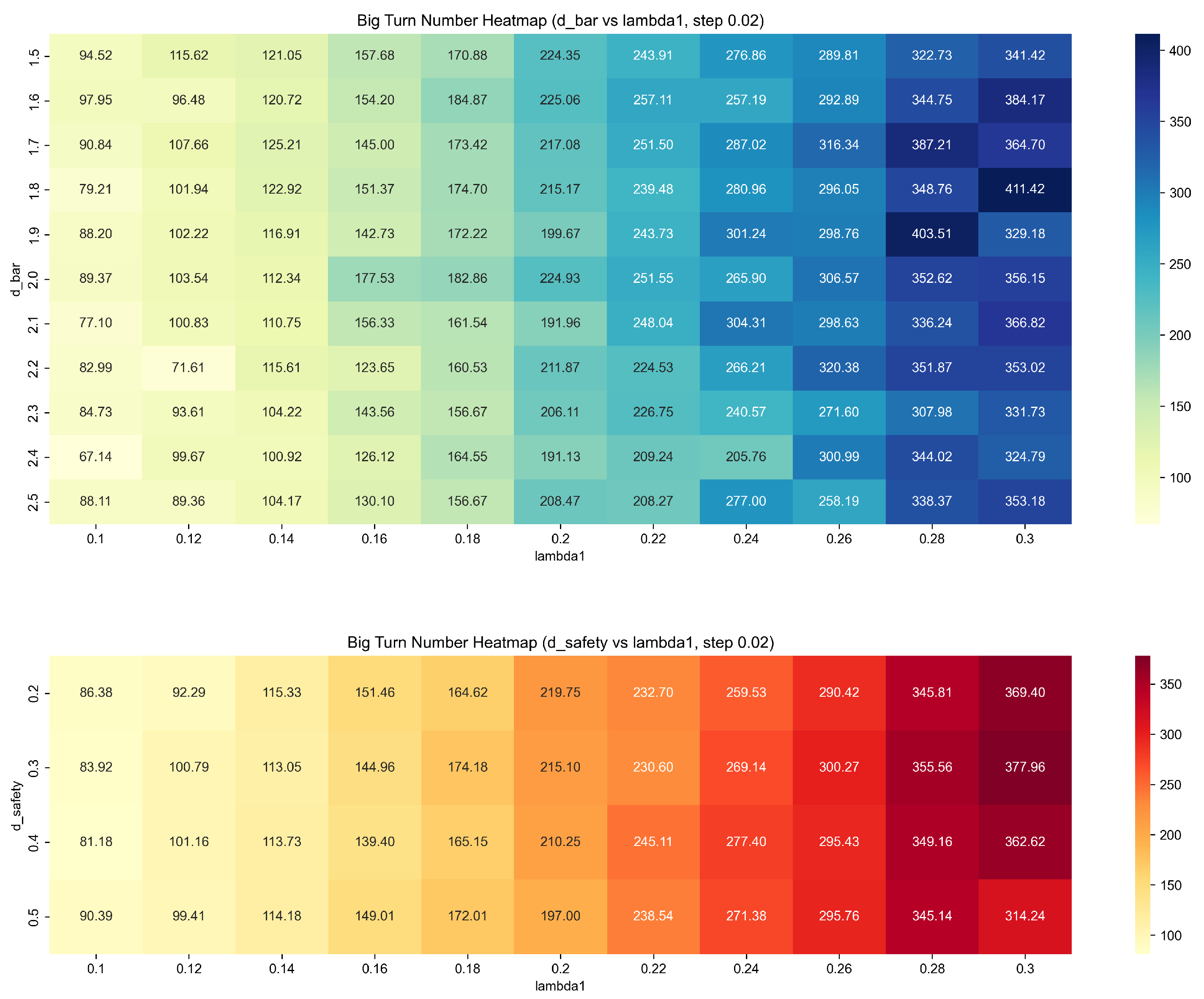
As shown in Figure 8, comparing the heatmaps of the number of sharp turns in the parameter planes of d_bar and lambda1, it can be observed that lambda1 has the most significant impact on the number of sharp turns, while d_bar has a certain degree of sensitivity, and the influence of d_safety is extremely limited. Therefore, in the actual parameter optimization process, lambda1 and d_bar should be adjusted first to obtain better path smoothness, while d_safety can be flexibly set according to safety requirements.

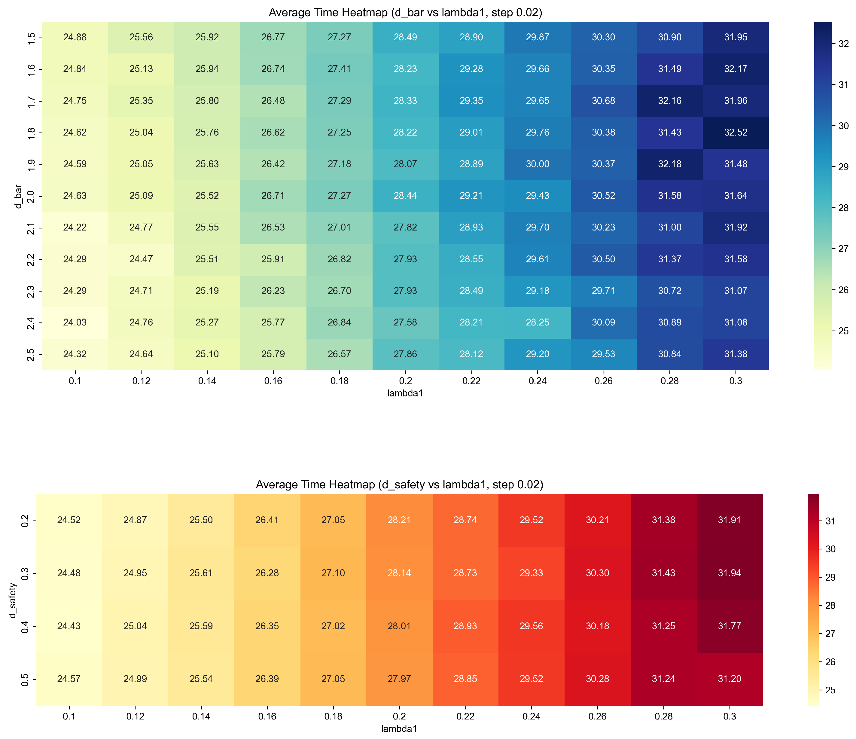
As shown in Figure 9, the heat map under the parameter plane of (d_bar, lambda1) and (d_safety, lambda1) was drawn. The results show that lambda1 has the most significant impact on the average time, and the average time increases significantly with the increase of lambda1, showing obvious monotonicity. d_bar has a certain influence on the average time, and an appropriate detection radius (such as 1.8 to 2.2) helps to improve efficiency, while d_safety has little effect on the average time, which can be set flexibly according to actual needs. On the whole, lambda1 and d_bar are the key parameters affecting the system efficiency, which should be optimized first in practical application.

The Figure 10 presents a heat map of the number of times trapped in local minima on the parameter plane of (d_bar, lambda1).

The results indicate that lambda1 has the most significant impact on the frequency of getting stuck in local minima. As lambda1 increases, the risk of being trapped in local minima significantly rises. d_bar also has a certain influence on this metric, with an appropriate detection radius (such as 1.8 to 2.2) helping to enhance the system’s global optimization capabilities. Overall, lambda1 and d_bar are the key parameters affecting the robustness of the system and should be optimized first in practical applications.

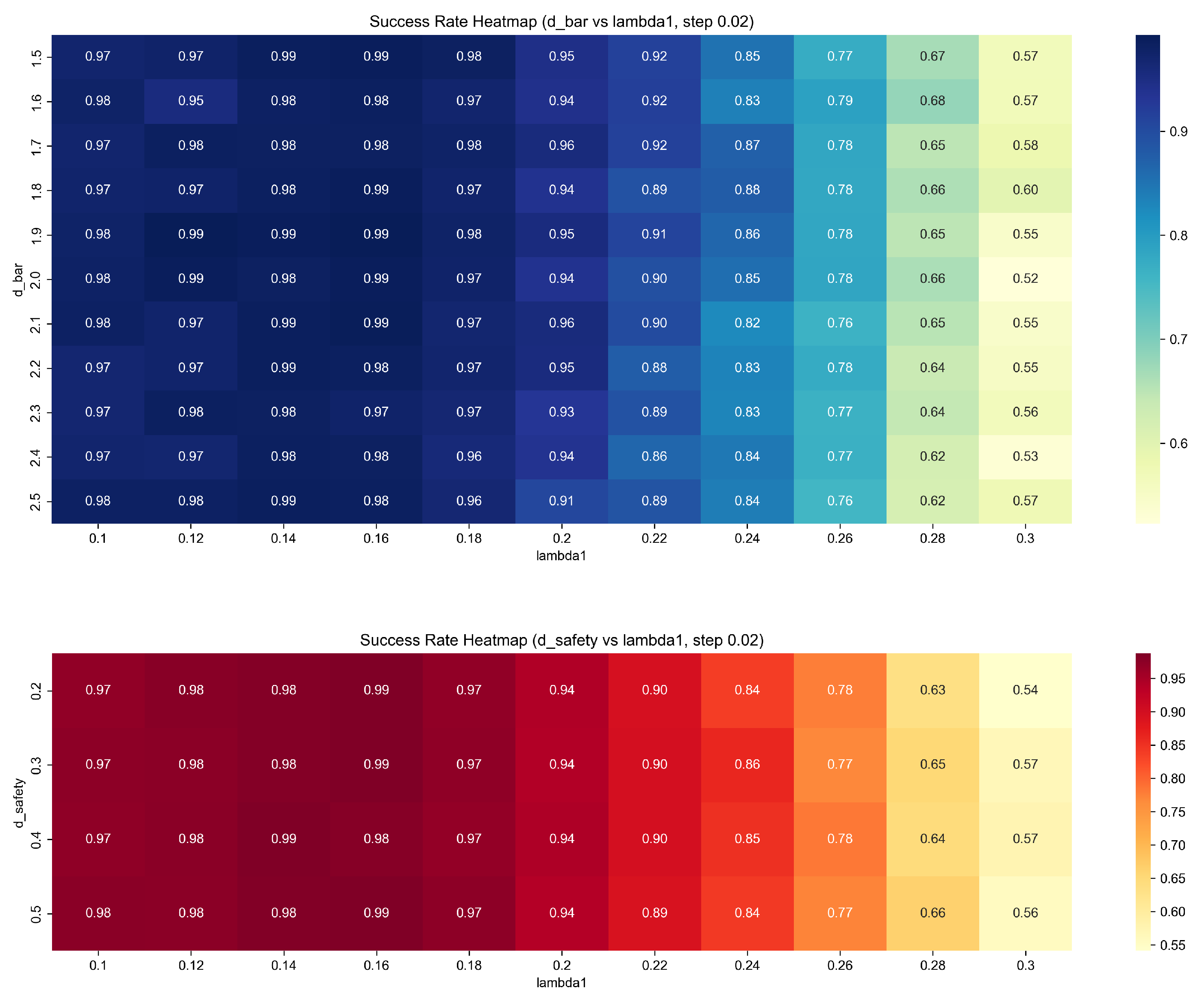
As shown in Figure 11, heatmaps of the success rate were plotted in the parameter planes of (d_bar, lambda1) and (d_safety, lambda1).

The results indicate that lambda1 has the most significant impact on the success rate. As lambda1 increases, the success rate significantly decreases. d_bar has a certain influence on the success rate, with an appropriate detection radius (such as 1.8 to 2.2) helping to enhance the robustness of the system. In contrast, d_safety has a minimal impact on the success rate and can be flexibly set according to actual needs. Overall, lambda1 and d_bar are the key parameters affecting the system’s success rate and should be prioritized for optimization in practical applications.

4.3. Evaluation Parameter Settings

During the experimental process, the traditional artificial potential field and the A* algorithm were used instead of the VAPF based on RL to achieve path planning for drones. The local minima problem was evaluated mainly through success rate, average arrival time, and local minima count. In a single path planning process, if the distance between all drones and their respective target positions was less than or equal to 0.1 m, the path planning was considered successful. The number of iterations at this point was recorded as the arrival time, and the actual arrival time was expressed as the product of the number of iterations and 0.02 s. 20 groups of 1000 experiments were run to calculate the success rate, average arrival time, and local minima.

Additionally, this paper designs the parameter local minima count to specifically evaluate the number of times the drone gets trapped in local minima. The evaluation criteria are as follows: In the navigation paths where the drone fails to reach the target, if the drone’s movement distance is less than 0.5 m within the last 50 steps and the target position is outside the detection range of the drone’s sensors, it is considered that the drone is trapped in a local minimum. Since the maximum movement speed of the drone is set to 2 m/s in this paper, and the average movement speed during the experiment reaches 1.8 m/s, one of the core characteristics of local minima is that the drone is physically unable to move forward, or moves very slowly, being “trapped” by obstacles. If the drone moves only a very small distance (less than 0.5 m) continuously over a period of time, this strongly indicates that it may be at a point of force balance, where the attraction and repulsion forces cancel each other out, or the resultant force is not enough to overcome inertia, resulting in almost no movement. The 50-step time window is used to distinguish between a normal brief pause of the drones, such as an abrupt stop during obstacle avoidance, and a persistent trapped state. At the same time, in the APF method, when the drone is surrounded by obstacles near the target, it often fails to detect the target while being repelled by the obstacles, leading to stagnation. Therefore, the local minima count parameter can effectively evaluate the local minima situation in path planning.

In the path planning process, smoothness is a crucial evaluation criterion, as it directly impacts the stability of movement, energy efficiency, control performance, equipment lifespan, and operational safety. A path that effectively avoids obstacles while maintaining smoothness is considered practical and efficient.

This study primarily assesses path smoothness using the number of sharp turns and average curvature. The design of the evaluation parameters is as follows. We only count the number of sharp turns and average curvature when the drone successfully reaches the target location. To eliminate the influence of initial instability in the drone’s control system, the first 10 time steps of the trajectory are not considered. A sharp turn is recorded when the curvature of the drone’s trajectory exceeds a certain threshold, indicating a significant change in direction.

4.4. Experimental Results Analysis

4.4.1. Local Minimum Value

By comparing the navigation performance of the three methods under different obstacle environments, we found that when the obstacles are relatively dispersed, all three algorithms effectively complete the path planning task. Although the A* algorithm is relatively mature, the VAPF based on RL designed in this study excels in solving the problem of local minima. The specific results are shown in

Table 2. Local minimum evaluation parameters.

Controller	Successful Rate	Average Time (s)	Local Minima Count
A*	0.975	27.5	40
APF	0.979	27.1	23
VAPF	0.985	26.27	5

.

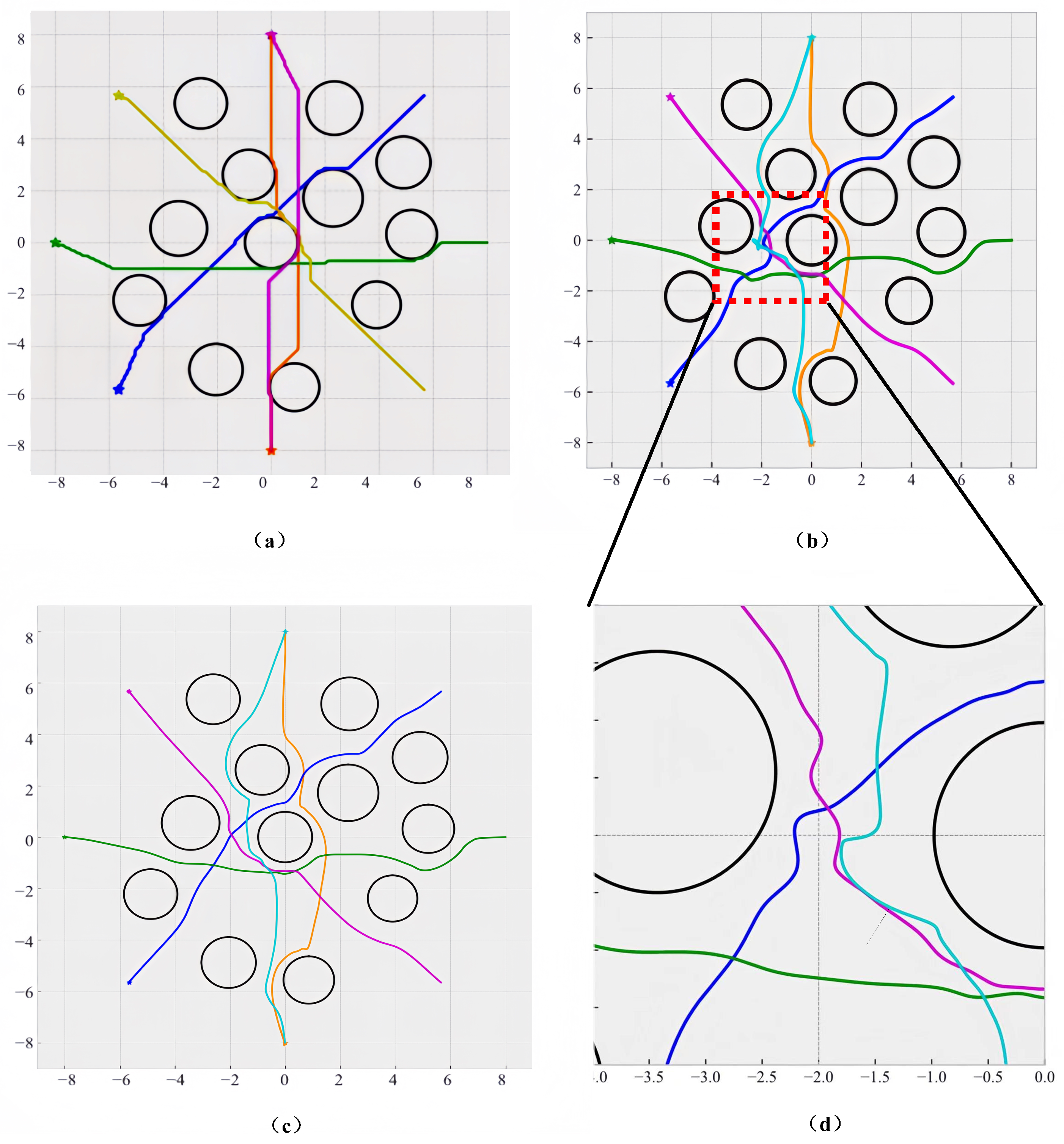
Compared with the traditional APF, the VAPF based on RL effectively solves the problem of local minima. The path diagram is shown in Figure 12.

The reason lies in the introduction of vortex repulsive force in the method of VAPF based on RL, which is equivalent to adding a perturbation term to the original force balance equation. When the vortex repulsive force is not exactly opposite to the existing resultant force or points in an ineffective direction, the original balance is broken, and the resultant force is no longer zero or ineffective, so the drone will not fall into local minima. However, when the vortex repulsive force completely cancels out the existing resultant force or points in an ineffective direction, the original balance is not broken, and there is a possibility that the drone may fall into local minima.

4.4.2. Path Smoothness

In the path planning process, smoothness is a crucial evaluation criterion, as it directly impacts the stability of movement, energy efficiency, control performance, equipment lifespan, and operational safety. A path that effectively avoids obstacles while maintaining smoothness is considered practical and efficient. By comparing the performance of three methods in various obstacle-filled environments, we observe that the VAPF based on RL not only outperforms in resolving local minimum issues but also reduces the turning rate and the number of sharp turns compared to the other methods, resulting in a smoother path. The A* algorithm’s discrete search nature and its focus on optimizing only the path length limit its capability to generate smooth trajectories. On the other hand, the VAPF based on RL, by operating in a more continuous space, optimizing a multi-objective reward function that includes smoothness, and utilizing a detailed potential field model for navigation control, naturally learns to produce smoother, more continuous paths. The specific results are shown in

Table 3. Path smoothness evaluation parameters. The unit of average turning rate is m⁻¹.

Controller	Average Curvature	Big Turn Number
A*	2547	120
APF	2700	167
VAPF	2689	94

.

4.4.3. Comparison of Reinforcement Learning Algorithms

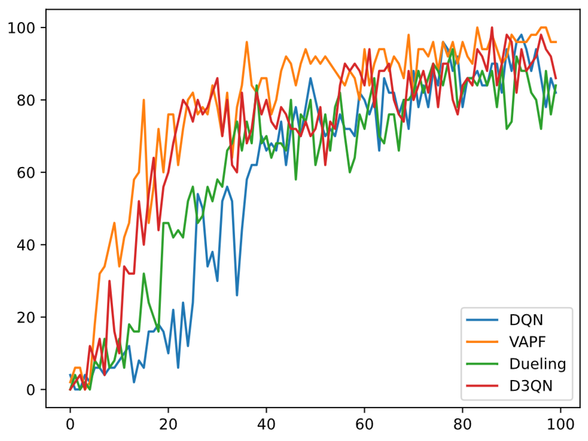
The DQN algorithm is a widely used reinforcement learning method. To effectively compare the VAPF algorithm with other reinforcement learning algorithms, this study evaluates the training performance of four algorithms (DQN, VAPF, Dueling DQN, and D3QN) in path planning tasks. As depicted in the figure, the x-axis indicates the training phase number, with each number corresponding to a saved model, thereby reflecting training progress. The y-axis shows the success rate of each model on a standard test set, which is the average success rate over 50 tests, ranging from 0 to 1.

In the Figure 13, the blue curve represents the basic DQN, the orange curve denotes the VAPF method used in this study, the green curve illustrates the Dueling DQN variant with an advantage value separation structure, and the red curve depicts the D3QN variant integrating Double and Dueling concepts.

Throughout the training process, the success rates of all four algorithms significantly improve with increasing training rounds, indicating continuous learning and strategy optimization. Ultimately, all algorithms achieve success rates above 0.8, demonstrating robust path planning capabilities. VAPF and D3QN exhibit rapid initial improvement (within the first 20 rounds), with success rates rising early, showcasing quicker convergence.

DQN and Dueling DQN show greater volatility in the early stages, with slower initial improvement, but they eventually stabilize at higher success rates. VAPF and D3QN perform more consistently in the later stages (post-40 rounds), with minimal fluctuations and sustained high success rates. DQN and Dueling DQN experience more variability in the mid-stage (20–60 rounds), with occasional dips, but they also converge to higher success rates over time.

The experimental results indicate that the VAPF and D3QN algorithms excel in learning and generalization for path planning tasks, achieving high success rates more quickly and consistently, with VAPF slightly outperforming D3QN in terms of success rate.

The performance of four control algorithms, DQN, VAPF, Dueling, and D3QN, was compared in a simulation environment. The

Table 4. Comparison of experimental data for reinforcement learning algorithms.

Controller	Successful Rate	Average Time (s)	Local Minima Count	Curvature	Big Turn Number
DQN	0.980	27.1	12	3457	154
VAPF	0.985	26.27	5	2689	94
Dueling	0.845	26.9	10	2894	144
D3QN	0.982	27.24	13	3541	105

show that the VAPF algorithm excels in all metrics, with a success rate of 0.985, an average time of 26.27 s, and only 5 local minima. Its average curvature and the number of sharp turns are also superior to other algorithms, with values of 2689 and 94, respectively. In contrast, DQN and D3QN also have high success rates, at 0.980 and 0.982, but they are slightly less effective than VAPF in terms of path smoothness and the number of sharp turns. The Dueling algorithm has the lowest success rate, only 0.845, and its overall performance is not as good as the other methods. Overall, the VAPF algorithm demonstrates stronger advantages and robustness in terms of path planning success rate, efficiency, and path quality.

4.4.4. Summary of Experimental Results

In summary, the VAPF based on RL learning introduces vortex repulsive force on the basis of the APF, which better solves the problem of local minima and improves the smoothness of the path to a certain extent. At the same time, compared with the A* algorithm, which can generate shorter paths in an ideal environment, in the actual application process, the VAPF based on RL has more obvious advantages due to its fast and reliable characteristics. These advantages make the VAPF based on RL more competitive in complex and changeable actual application environments and can provide more effective and reliable navigation strategies for drones.

5. Discussion

In this study, VAPF breaks the symmetric force balance of traditional APF by introducing a tangential force, fundamentally solving the problem of local minima. Experiments show that the perturbation mechanism of VAPF significantly reduces the risk of stagnation in densely obstacle-packed areas. The physical essence of this design lies in: the vortex repulsive force dynamically adjusts the virtual target coordinates, rather than directly acting on the drone, avoiding motion oscillation caused by force field interference. Compared with the repulsive function proposed by Garcia-Delgado et al., VAPF’s “indirect navigation” mechanism is more adaptable to dynamic obstacle environments.

By decomposing motion control into translation control and rotation control and independently training each dimensional controller through reinforcement learning, a balance between motion precision and obstacle avoidance flexibility is achieved. This design solves the problem of path jitter caused by sudden attitude changes in traditional methods. Experimental data show that this structure reduces the average number of turns, verifying its advantage in path smoothness.

Parameter sensitivity analysis reveals the vortex intensity parameter has the most significant impact on path success rate and local minima frequency, while the detection radius mainly affects path efficiency. This provides parameter tuning criteria for actual deployment: prioritize optimizing the vortex intensity parameter and detection radius, which can be flexibly set according to task risk. For example, in the logistics distribution scenario, a smaller radius is needed to reduce and improve efficiency, while post-disaster rescue needs to expand to ensure safety.

Although pure RL algorithms have success rates close to VAPF in the later stages of training, VAPF has advantages in convergence speed and stability. The reason is APF’s prior knowledge reduces the RL exploration space, avoiding waste on invalid actions. However, VAPF’s adaptability to dynamic targets depends on gradient calculations, and future online learning mechanisms can be introduced to deal with sudden obstacles.

6. Conclusions

The scheme proposed in this paper, which combines RL-based motion control with APF obstacle avoidance technology, provides a new approach for the design of autonomous navigation systems for drones. This method effectively addresses the limitations of traditional APF methods and demonstrates good obstacle avoidance performance and path planning efficiency. Future research can further explore the application of this method in more complex dynamic environments [28] and multi-target scenarios [29,30,31], and its combination with other control methods to enhance the drone’s motion control performance. The experiments in this paper were mainly conducted in relatively simple dynamic environments, and future research can investigate the application of this method in more complex dynamic environments. Additionally, the method proposed in this paper can be combined with other control methods [32] to further improve the drone’s motion control performance. Applying the method proposed in this paper to actual drone platforms and conducting test validations.

References

1. Huang, Y.; Thomson, S.J.; Hoffmann, W.C.; Lan, Y.; Fritz, B.K. Development and prospect of unmanned aerial vehicle technologies for agricultural production management. Int. J. Agric. Biol. Eng. 2013, 6, 1–10. [Google Scholar]
2. Lyu, M.; Zhao, Y.; Huang, C.; Huang, H. Unmanned aerial vehicles for search and rescue: A survey. Remote Sens. 2023, 15, 3266. [Google Scholar] [CrossRef]
3. Liu, Q.; Qi, Z.; Wang, S.; Liu, Q. Edge-Intelligence-Powered Joint Computation Offloading and Unmanned Aerial Vehicle Trajectory Optimization Strategy. Drones 2024, 8, 485. [Google Scholar] [CrossRef]
4. Wang, X.; Feng, Y.; Tang, J.; Dai, Z.; Zhao, W. A UAV path planning method based on the framework of multi-objective jellyfish search algorithm. Sci. Rep. 2024, 14, 28058. [Google Scholar] [CrossRef]
5. Bai, Y.; Li, K.; Wang, G. A Hybrid Quadrotor Unmanned Aerial Vehicle Control Strategy Using Self-Adaptive Bald Eagle Search and Fuzzy Logic. Electronics 2025, 14, 2112. [Google Scholar] [CrossRef]
6. Shakhatreh, H.; Sawalmeh, A.H.; Al-Fuqaha, A.; Dou, Z.; Almaita, E.; Khalil, I.; Othman, N.S.; Khreishah, A.; Guizani, M. Unmanned aerial vehicles (UAVs): A survey on civil applications and key research challenges. IEEE Access 2019, 7, 48572–48634. [Google Scholar] [CrossRef]
7. Yan, Z.; Jouandeau, N.; Cherif, A.A. A survey and analysis of multi-robot coordination. Int. J. Adv. Robot. Syst. 2013, 10, 399. [Google Scholar] [CrossRef]
8. Jiang, Y.; Gao, Y.; Song, W.; Li, Y.; Quan, Q.U. Bibliometric analysis of UAV swarms. J. Syst. Eng. Electron. 2022, 33, 406–425. [Google Scholar] [CrossRef]
9. Agarwal, V.; Tapaswi, S.; Chanak, P. A Survey on Path Planning Techniques for Mobile Sink in IoT-Enabled Wireless Sensor Networks. Wirel. Pers. Commun. 2021, 119, 1–28. [Google Scholar] [CrossRef]
10. Kavraki, L.E.; Svestka, P.; Latombe, J.C.; Overmars, M.H. Probabilistic roadmaps for path planning in high-dimensional configuration spaces. IEEE Trans. Robot. Autom. 1996, 12, 566–580. [Google Scholar] [CrossRef]
11. Zheng, L.; Wang, X.; Li, F.; Mao, Z.; Tian, Z.; Peng, Y.; Yuan, F.; Yuan, C. A Mean-Field-Game-Integrated MPC-QP Framework for Collision-Free Multi-Vehicle Control. Drones 2025, 9, 375. [Google Scholar] [CrossRef]
12. Liu, Z.; Zhang, Z. The Research on an Improved YOLOX-Based Algorithm for Small-Object Road Vehicle Detection. Electronics 2025, 14, 2179. [Google Scholar] [CrossRef]
13. Lin, Y.; Gao, H.; Xia, Y. Distributed Pursuit–Evasion Game Decision-Making Based on Multi-Agent Deep Reinforcement Learning. Electronics 2025, 14, 2141. [Google Scholar] [CrossRef]
14. Tang, L.; Dian, S.; Gu, G.; Zhou, K.; Wang, S.; Feng, X. A novel potential field method for obstacle avoidance and path planning of mobile robot. In Proceedings of the 2010 3rd International Conference on Computer Science and Information Technology, Wuxi, China, 4–6 June 2010; Volume 9, pp. 633–637. [Google Scholar]
15. Jin, F.; Ye, Z.; Li, M.; Xiao, H.; Zeng, W.; Wen, L. A New Hybrid Reinforcement Learning with Artificial Potential Field Method for UAV Target Search. Sensors 2025, 25, 2796. [Google Scholar] [CrossRef]
16. Khatib, O. Real-time obstacle avoidance for manipulators and mobile robots. Int. J. Robot. Res. 1986, 5, 90–98. [Google Scholar] [CrossRef]
17. Guldner, J.; Utkin, V.I.; Hashimoto, H. Robot obstacle avoidance in n-dimensional space using planar harmonic artificial potential fields. In Proceedings of the 1997 International Conference on Robotics and Automation, Albuquerque, NM, USA, 21–27 April 1997; pp. 160–166. [Google Scholar]
18. Keyu, L.; Yonggen, L.; Yanchi, Z. Dynamic obstacle avoidance path planning of UAV Based on improved APF. In Proceedings of the 2020 5th International Conference on Communication, Image and Signal Processing (CCISP), Chengdu, China, 13–15 November 2020; pp. 159–163. [Google Scholar]
19. Zhang, B.; Lv, M.; Cui, S.; Bu, X.; Park, J.H. Learning-based optimal cooperative formation tracking control for multiple UAVs: A feedforward-feedback design framework. IEEE Trans. Autom. Sci. Eng. 2025, 22, 123–135. [Google Scholar] [CrossRef]
20. Gao, X.; Zhang, Y.; Wang, B.; Leng, Z.; Hou, Z. The Optimal Strategies of Maneuver Decision in Air Combat of UCAV Based on the Improved TD3 Algorithm. Drones 2024, 8, 501. [Google Scholar] [CrossRef]
21. Park, D.H.; Hoffmann, H.; Pastor, P.; Schaal, S. Movement reproduction and obstacle avoidance with dynamic movement primitives and potential fields. In Proceedings of the 2008 8th IEEE-RAS International Conference on Humanoid Robots (HUMANOIDS 2008), Daejeon, Republic of Korea, 1–3 December 2008; pp. 91–98. [Google Scholar]
22. Phang, R.C.; Hirata, A. Shared autonomy between human electroencephalography and TD3 deep reinforcement learning: A multi-agent copilot approach. Ann. N. Y. Acad. Sci. 2025, 1546, 157–172. [Google Scholar] [CrossRef]
23. Zhang, J.; Li, F.; Li, J.; Chen, Q.; Sheng, H. A Pseudo-Exponential-Based Artificial Potential Field Method for UAV Cluster Control under Static and Dynamical Obstacles. Drones 2024, 8, 506. [Google Scholar] [CrossRef]
24. Han, H.; Xi, Z.; Lv, M.; Cheng, J. Acceleration of formation control based on hessian matrix of artificial potential field. In Proceedings of the 2023 42nd Chinese Control Conference (CCC), Tianjin, China, 24–26 July 2023; pp. 5866–5871. [Google Scholar]
25. Rong, W.; Zheng, J.; Chen, Y.; Liu, Y.; Zhang, Z. Autonomous collision avoidance decision-making method with human-like attention distribution for MASSs based on GMA-TD3 algorithm. Ocean. Eng. 2025, 330, 121118. [Google Scholar] [CrossRef]
26. Goodarzi, F.; Lee, D.; Lee, T. Geometric nonlinear PID control of a quadrotor UAV on SE (3). In Proceedings of the 2013 European Control Conference (ECC), Zurich, Switzerland, 17–19 July 2013; pp. 3845–3850. [Google Scholar]
27. García-Delgado, L.A.; Noriega, J.R.; Berman-Mendoza, D.; Leal-Cruz, A.L.; Vera-Marquina, A.; Gómez-Fuentes, R.; García-Juárez, A.; Rojas-Hernández, A.G.; Zaldívar-Huerta, I.E. Repulsive function in potential field based control with algorithm for safer avoidance. J. Intell. Robot. Syst. 2015, 80, 59–70. [Google Scholar] [CrossRef]
28. Lv, M.; Ahn, C.K.; Zhang, B.; Fu, A. Fixed-time antisaturation cooperative control for networked fixed-wing unmanned aerial vehicles considering actuator failures. IEEE Trans. Aerosp. Electron. Syst. 2023, 59, 6545–6558. [Google Scholar] [CrossRef]
29. Lv, M.; Yu, W.; Cao, J.; Baldi, S. Consensus in high-power multiagent systems with mixed unknown control directions via hybrid Nussbaum-based control. IEEE Trans. Cybern. 2022, 52, 5009–5020. [Google Scholar] [CrossRef]
30. Zhang, B.; Sun, X.; Liu, S.; Lv, M.; Deng, X. Event-triggered adaptive fault-tolerant synchronization tracking control for multiple 6-DOF fixed-wing UAVs. IEEE Trans. Veh. Technol. 2022, 71, 123–135. [Google Scholar] [CrossRef]
31. Lv, M.; Wang, N. Distributed control for uncertain multiagent systems with the powers of positive-odd numbers: A low-complexity design approach. IEEE Trans. Autom. Control. 2024, 69, 123–135. [Google Scholar] [CrossRef]
32. Lv, M.; Yu, W.; Cao, J.; Baldi, S. A separation-based methodology to consensus tracking of switched high-order nonlinear multiagent systems. IEEE Trans. Neural Netw. Learn. Syst. 2022, 33, 1234–1245. [Google Scholar] [CrossRef]
Figure 2. Schematic diagram of the three-axis attitude angles of a quadrotor drone.
Machines 13 00600 g002
Figure 3. Schematic diagram of relative positioning and obstacle avoidance for quadcopter drones.
Machines 13 00600 g003
Figure 4. The velocity of the drone is constrained to lie inside a circular region centered on the origin with radius V e .
Machines 13 00600 g004
Figure 5. Decomposition of drone vortex repulsive force: one generated by drones on their collision path ( w 2 ), and the other by drones not on their collision path ( w 3 ).
Machines 13 00600 g005
Figure 6. TD3 algorithm flowchart.
Machines 13 00600 g006
Figure 7. Isotropy diagram.
Machines 13 00600 g007
Figure 8. Heatmap of the big turn number.
Machines 13 00600 g008
Figure 9. Heatmap of the average time.
Machines 13 00600 g009
Figure 10. Heatmap of local minima.
Machines 13 00600 g010
Figure 11. Heatmap of the success rate.
Machines 13 00600 g011
Figure 12. (a) illustrates the path planned using the traditional A* algorithm, (b) shows the path planned with the APF method, (c) presents the path planned using VAPF, and (d) is a detailed view of the APF path planning map.
Machines 13 00600 g012
Figure 13. The figure illustrates the success rates of four reinforcement learning algorithms throughout the training process.
Machines 13 00600 g013