Deploying an Educational Mobile Robot

Abstract

This study presents the development of a software solution for processing, analyzing, and visualizing sensor data collected by an educational mobile robot. The focus is on statistical analysis and identifying correlations between diverse datasets. The research utilized the PlatypOUs mobile robot platform, equipped with odometry and inertial measurement units (IMUs), to gather comprehensive motion data. To enhance the reliability and interpretability of the data, advanced data processing techniques—such as moving averages, correlation analysis, and exponential smoothing—were employed. Python-based tools, including Matplotlib and Visual Studio Code, were used for data visualization and analysis. The analysis provided key insights into the robot’s motion dynamics; specifically, its stability during linear movements and variability during turns. By applying moving average filtering and exponential smoothing, noise in the sensor data was significantly reduced, enabling clearer identification of motion patterns. Correlation analysis revealed meaningful relationships between velocity and acceleration during various motion states. These findings underscore the value of advanced data processing techniques in improving the performance and reliability of educational mobile robots. The insights gained in this pilot project contribute to the optimization of navigation algorithms and motion control systems, enhancing the robot’s future potential in STEM education applications.

1. Introduction

Modern engineering education needs to supply the new needs of the industry, following the Industry 4.0 revolution. All segments and professions are striving to gain a boost from new technologies, such as cloud computing, the Internet of Things, and artificial intelligence (AI) [1,2]. New methods are inspiring innovation and exploitation, cross-fertilized by the combination of machine learning (ML)/AI, robotics, and big data technologies. The OECD’s definition for an AI system emphasizes the human-defined objectives, the ability to make predictions, recommendations, and the capability of influencing real or virtual environments [3], while robots are defined by Haidegger as being a complex mechatronic system enabled with electronics, sensors, actuators, and software that executes tasks with a certain degree of autonomy [4]. Meanwhile, big data and data science are the study of data analysis by advanced technology, processing a huge amount of structured, semi-structured, and unstructured data [5,6].

Mobile robots serve as excellent tools for educators across various engineering fields, facilitating the implementation of skill development tasks [5,7]. The complexity of these systems provides valuable insights into how new technologies can be integrated to enhance system efficiency, reduce energy consumption, and improve materials and techniques. Numerous studies in the literature highlight the use of mobile robotic platforms in educational settings, demonstrating how they improve student learning and training in robotics by providing hands-on experience with physical platforms [8,9].

Recent advancements in educational mobile robots have significantly improved their capabilities, leading to increased adoption in educational institutions, including schools and universities. These robots can perform a wide range of tasks, from teaching basic programming to tackling more advanced engineering challenges. Notable examples include LEGO Mindstorms, which enables students and teachers to build and program their own robots while learning about mechanics, electronics, and software development. Dash and Dot, designed for younger learners, teach programming concepts in a playful and engaging manner. Additionally, TurtleBot serves as a popular educational tool, helping students grasp the fundamentals of robotics and artificial intelligence. The widespread use and versatility of mobile robots open up new educational opportunities and help students develop critical technology and engineering skills [8,10].

Despite their growing popularity, educational mobile robots still face challenges in sensor data analysis, motion control optimization, and navigation accuracy. Sensor data often contain noise and inconsistencies that impede accurate interpretation. Moreover, the lack of standardized tools for processing and visualizing sensor data limits the ability to identify patterns and trends effectively. Statistical analysis techniques, including moving averages, variance analysis, correlation studies, and exponential smoothing, are commonly used in mobile robotics to reduce noise, identify trends, and enhance data reliability. However, these methods often require manual implementation and lack integration into user-friendly software solutions tailored to educational purposes.

This study addresses these challenges by developing a modular software solution for processing, analyzing, and visualizing sensor data collected by the PlatypOUs mobile robot platform. The proposed system integrates statistical methods such as moving averages, correlation analysis, and exponential smoothing to improve data reliability and interpretability. By bridging the gap between raw sensor data and actionable insights, this research aims to optimize robot performance and support STEM education.

RVIZ is a comprehensive 3D visualization tool for robots using ROS [11,12]. It effectively displays sensor data and robot state information by combining and presenting it all in a single image overlaid on a simulated environment. However, a notable limitation of RVIZ is its lack of access to raw data, making it difficult for developers to interpret the underlying information directly. One potential solution is to enhance RVIZ with markers. Markers are simulated objects within the visualization that can be programmatically sized and positioned. For example, they can be used to represent radial lines from a laser scan or place cubes whose height corresponds to the robot’s current speed [13,14,15].

Alternatively, augmented reality offers another approach, as demonstrated by Collet and MacDonald [16]. Their work focuses on representing data within a real-world environment, using examples like laser and sonar scans.

In the domain of live programming, several languages feature their own visualizations. The concept of live programming dates back to Tanimoto’s work on VIVA [17], a programming language for image processing that uses a graphical representation of programs, similar to electronic circuits, with data flowing along wires to processing components. A similar data-flow-based approach is seen in Hancock [18], a live programming language designed for teaching robotics, where sensor readings are displayed as numerical or Boolean data that are easy to interpret without the need for additional visualizations.

Using the PlatypOUs platform (0.2.0) (Figure 1), the simulator offers students and self-study participants hands-on experience and teaches them to tackle complex engineering problems in a professional yet engaging way [19]. The open-source mobile robot platform can be remotely controlled by an electromyography (EEG) device (https://mindrove.com/product/eeg-headset/ accessed on 2 July 2025) using the MindRove Arc 2 6-channel brain–computer interface headset. The collected bio-signals are classified using a support vector machine, and the results provide motion instructions to the mobile platform. In addition to the real robot, a virtual environment has been created in Gazebo, offering the same capabilities as the physical device. The PlatypOUs project aims to support STEM education and extracurricular activities, particularly laboratory exercises and demonstrations. It spans several disciplines, including systems design, control engineering, mobile robotics, and machine learning, with applications in all these fields. The PlatypOUs platform was developed to serve as both a research and educational tool for sensor-based robot control tasks [20]. It also offers a platform for experimenting with other emerging control modalities, such as augmented reality headsets and eye-gaze tracking [21].

The main contributions of our work include the development of a modular system that demonstrates robot sensorics and control functions across various education levels, along with the prototyping and testing activities conducted during the research. The features of our system related to sensory data collection and aggregation are summarized in

Table 1. Comparison of types of data that can be obtained from PlatypOUs and ROS-RVIZ-Gazebo.

Type of Data	PlatypOUs Data	ROS-RVIZ-Gazebo Data
Odometry Data (Wheel Encoders)	Provides position (x, y), orientation (theta), linear velocity (m/s), and angular velocity (rad/s) from wheel encoders.	Typically, only position and orientation are available in RVIZ. Raw encoder data may not be accessible.
IMU Data (Gyroscope and Accelerometer)	Records angular velocities (gyro_x, gyro_y, gyro_z) and linear accelerations (acc_x, acc_y, acc_z) at a frequency of 200 Hz.	RVIZ displays visualized data, but raw IMU data such as angular velocities and accelerations are not directly accessible in standard setups.
Correlation Analysis Between Sensors	Provides correlation data between velocity, acceleration, and sensor outputs to optimize navigation and sensor systems.	RVIZ does not provide direct access to raw sensor data for in-depth correlation analysis.
Moving Average Filtering of Sensor Data	Uses moving average techniques to smooth data and reduce noise in odometry and IMU readings for improved stability.	RVIZ is used for visualization and does not provide tools for directly applying data processing techniques like moving averages on raw sensor data.
Exponential Smoothing of Sensor Data	Applies exponential smoothing to reduce noise and better reflect actual motion dynamics (e.g., gyroscope and accelerometer data).	RVIZ does not apply exponential smoothing to sensor data for noise reduction.
Sensor Fusion and Multi-sensor Integration	Integrates multiple sensors (odometry, IMU) and processes their data for a comprehensive understanding of robot motion and behavior.	RVIZ visualizes the data but does not process multi-sensor fusion or provide direct access to combine sensor data.

.

2. Materials and Methods

2.1. Robotics and Automation

For the education of the next digital native generation, the question is how robotics and AI tools can play an effective role in educational work and what positive effects can be highlighted in terms of development in educational processes, taking into account the constant change, which is one of the most important factors in the current era of digitalization [22,23]. Robotic megatrends outline the key research and educational aspects of our time, from the most critical applications—like surgery—to robot toys [24,25,26]. Computer science and programming education and robotics play an important role in technical higher education. Developing programming skills is a priority for all students. Algorithmic thinking and problem-solving skills are particularly important. The tools to achieve the above objectives are the Webots development environment and Parallax’s Boe-bot programmable robot [27].

2.2. Mobile Robots in Education

C/C++ programming languages are commonly used to teach the fundamentals of robot programming, after which students can expand their knowledge to languages such as C#, Java, PHP, and others. In educational settings, programmable robots like Boe-bot are valuable tools for students of varying ages and skill levels. These robots provide an engaging and interactive way to learn programming, offering students the opportunity to apply theoretical knowledge in real-world scenarios. Programming in real-life contexts allows for the testing of different programming languages and environments. Furthermore, these robots can serve as teaching aids in a variety of subjects, including communication, artificial intelligence, image processing, algorithm theory, shape recognition, game theory, and swarm intelligence. Their versatility in education makes mobile robots an essential component of modern learning tools.

The PlatypOUs robot is a differential drive mobile platform, equipped with two driven wheels powered by brushless DC hub motors. These motors are controlled by an ODrive BLDC driver board, an open-source motor control solution with freely available schematics and firmware. The driver board communicates with the robot’s main computer, an Intel NUC8i5BEH mini PC, via a USB-Serial interface (https://intelnuc.co.in/intel-nuc-kit-with-8th-generation/intel-nuc-kit-nuc8i5beh/ accessed on 2 July 2025).

The robot is powered by two 24 V, 15 Ah Li-ion battery packs connected in parallel. While the motor driver board receives full battery voltage, the main computer and sensors are powered at 12 V or 5 V through voltage regulators. Safety features include fuses on all power lines, a main power switch, and an emergency switch. The emergency switch disconnects only the motor driver, preventing movement while ensuring the computer remains operational.

Our system is equipped with a range of sensors, including a YDLIDAR X4 laser scanner (https://www.ydlidar.com/product/ydlidar-x4-pro accessed on 2 July 2025), an Intel RealSense D455 depth camera (https://www.intelrealsense.com/depth-camera-d455/ accessed on 2 July 2025), and wheel encoders. These sensors collect environmental data, allowing the robot to map its surroundings, determine its precise location, detect obstacles, and navigate autonomously to target destinations.

2.3. Limitations of Prior Art

RViz is a standard visualization tool in ROS-based robotics education [11]. It focuses primarily on the live 3D visualization of robot states and does not provide access to raw sensor data for detailed analysis. Simulation environments like Gazebo are focused on replicating physical environments and robot dynamics but offer limited built-in tools for time-series data analysis and correlation inspection of sensor signals. Additionally, while platforms like LEGO Mindstorms and TurtleBot are effective for introductory robotics, they often provide black-box abstractions, limiting students’ exposure to the details of sensor data interpretation and filtering.

Visual programming environments like VIVA [17] and Flogo I [18] support flow-based or block-based learning but are not designed for analyzing physical sensor data from real robots. It seemed practical to take a new approach, integrating live coding in Python (3.9) with direct data pipeline manipulation, providing an authentic data science experience within robotics education—a key differentiator from visual-only programming tools.

3. Data Processing and Visualization

Data processing and visualization are critical components of mobile robotics applications, as the data collected by sensors can provide valuable insights [19]. Various methods, such as filtering, noise reduction, normalization, and transformation, can be used to process these data. Data visualization—the graphical representation and interpretation of data—has become an essential tool in natural sciences, social sciences, and engineering. The evolution of data visualization closely follows the development of application domains. While new types of diagrams, often minor variations of existing ones, continue to emerge in the field, more challenging areas involve the efficient and accurate visualization of large datasets, commonly referred to as ‘big data’ problems. Ultimately, data visualization aids in understanding data and facilitating communication, playing a pivotal role in scientific research, business decision-making, and other fields where data need to be interpreted and visualized [28,29].

As the volume, variety, and sources of data within organizations continue to grow, so does the importance of leveraging these data in analytics, data science, and machine learning initiatives to generate actionable business insights. This increasing demand is placing significant pressure on data engineering teams, as transforming raw, unstructured data into clean, reliable datasets is a critical step in enabling these systems to deliver valuable results. The ETL process—Extract, Transform, and Load—is used by data engineers to extract data from various sources, transform them into a usable and reliable format, and then load them into systems that end users can access to solve business problems [11,13,16,30].

3.1. Visual Studio Code

Visual Studio Code (1.86) is a free code editor that helps to get started with coding quickly. Visual Studio Code supports a wide range of languages, including Python, Java, C++ and JavaScript. While coding, Visual Studio Code provides suggestions for completing lines of code and quickly fixing common errors. VS Code’s debugger can also be used to go through each line of code and understand what is happening. The editor has all the standard tools expectable from a modern code editor, including syntax highlighting, customizable keyboard shortcuts, bracket insertion, and snippets. It runs on all operating systems, including Windows, Linus, and macOS [31].

3.2. Microsoft Power BI

Power BI (2024) is a business analytics service developed by Microsoft. It provides interactive business and business intelligence capabilities in an interface that is easy to use to create reports and dashboards. It makes it possible to connect to multiple data sources, clean and transform data, create customized calculations, and visualize data using charts, graphs, and tables. Power BI can be accessed through a web browser, on a mobile device, or as a desktop application, and can be integrated with other Microsoft tools such as Excel and SharePoint. It can be used for advanced data modeling and analysis capabilities, and organizations can use it to make data-driven decisions and gain insight into their business performance [31].

3.3. Matplotlib Library

Matplotlib (3.9) is a versatile data visualization library for Python, which makes it possible to create different types of graphs (histograms, scatter plots, bar charts) in cooperation with NumPy. Developers can use Matplotlib’s APIs (Application Programming Interfaces) to incorporate graphs into GUI (Graphical User Interface) applications. A typical Python Matplotlib script usually requires only a few lines of code to visualize the data. Matplotlib includes two main APIs for graphical representation:

• The pyplot API, which is a hierarchy of Python code objects, with matplotlib.pyplot representing the top level.
• An object-oriented (OO) API offering a collection of objects, providing more flexibility than pyplot. This API has direct access to the Matplotlib backend system [32].

We chose VS Code because it is ideal for both sensor data analysis and visualization as it is extremely user-friendly. As mentioned before, although it supports several programming languages, the Python was our preferred option. This platform is particularly suitable for handling large amounts of data and the built-in version tracking capabilities make it easier to organize and manage data analysis projects. Visual Studio Code is not only outstanding for its features, but also for its vast documentation, which provides support and guidance to users. It features powerful debugging tools, which are essential to quickly identify and solve problems that arise during data analysis processes.

3.4. Methods

The data were collected using a robot called PlatypOUs, which collects data using sensors. The data were saved in different CSV files. In the wheels odometry, data were calculated from the encoders and saved in the file wheel_odom.csv with a frequency of 100 Hz, in the following format:

• t: UNIX timestamp
• x: position x coordinate
• y: position y coordinate
• theta: orientation angle
• v: linear velocity
• omega: angular velocity

Brushless DC (BLDC) hub wheels with integrated 12-bit wheel encoders are advanced components used in differential drive platforms to provide precise wheel odometry measurements. These hub wheels incorporate BLDC motors, which offer high efficiency, low maintenance, and smooth operation. Additionally, the integrated encoders provide a resolution of 4096 counts per revolution (12 bits), allowing for fine-grained measurement of wheel rotations. The wheel encoders play a crucial role in determining the position and speed of each wheel by measuring the rotation in small increments.

To calculate the movement of a differential drive platform using encoder values, the control system reads the encoder ticks from each wheel. The distance traveled by each wheel is determined by multiplying the number of encoder ticks by the wheel circumference and dividing by the encoder resolution. In a differential drive system, the robot’s linear and angular movements are derived from the distances traveled by the left and right wheels. The forward movement is the average of the distances traveled by both wheels, calculated as the sum of the left and right distances divided by two. The change in orientation is determined by the difference in distances divided by the wheelbase width.

These calculations enable precise control of the robot’s trajectory by continuously updating its position and heading based on the encoder data. The integration of BLDC hub wheels with high-resolution encoders significantly enhances the accuracy and reliability of autonomous navigation in differential drive platforms.

The IMU measurements were saved in the file imu.csv, at a frequency of 200 Hz, in the following format:

• t: UNIX timestamp (nanosec)
• gyro_r: x-axis angular velocity
• gyro_y: y-axis angular velocity
• gyro_z: z-axis angular velocity
• acc_r: x-axis linear acceleration
• acc_y: y-axis linear acceleration
• acc_z: z-axis linear acceleration

Bosch BMI055 is a high-performance inertial measurement unit (IMU) designed for precise motion tracking and orientation sensing applications. It integrates a 3-axis accelerometer and a 3-axis gyroscope into a compact 3.0 × 4.5 × 0.95 mm LGA package, making it suitable for a wide range of applications, including mobile devices, gaming, and industrial control. The accelerometer in BMI055 features selectable measurement ranges of ±2 g, ±4 g, ±8 g, and ±16 g, with a sensitivity of 16,384 LSB/g in the ±2 g range and a noise density of 150 μg/√Hz. The gyroscope offers measurement ranges of ±125°/s, ±250°/s, ±500°/s, ±1000°/s, and ±2000°/s, with a sensitivity of 262.4 LSB/°/s in the ±125°/s range and a noise density of 0.014°/s/√Hz. The device operates over a supply voltage range of 2.4 to 3.6 V and supports both I2C and SPI digital interfaces, ensuring versatile integration into various systems. Additionally, BMI055 boasts low power consumption, with typical values of 0.14 mA for the accelerometer and 5.9 mA for the gyroscope, making it an efficient choice for battery-powered applications. With its high precision, low noise, and robust design, Bosch BMI055 IMU is well-suited for demanding applications requiring accurate and reliable inertial sensing.

4. Results

Various analyses can be performed on the data, making these calculations easier, such as:

Position and orientation tracking:

The current position and orientation of the robot, based on the odometry data.

Velocity and acceleration analysis:

Tracking the robot’s linear and angular velocity and linear robot motion and acceleration to identify motion patterns, turns, and accelerations.

The robot’s speed and direction of rotation:

• Analysis of IMU data: using IMU gyroscope data to determine the robot’s rotational speed and direction. IMU linear acceleration data can help navigate terrain and avoid collisions with obstacles.

The analyses performed on the data include:

• Moving averages: As a statistical method to move a set of values from a dataset within a given time interval or window. It is a technique that is often used to smooth time series or to determine trends. It can be used to reduce the variability of data and reveal long-term patterns.
• Scattering: Helps to understand how far data spread from the mean. It helps to understand the distribution of the variance from the mean. This is particularly important in assessing the stability and reliability of sensor data. Scatter can also be useful for checking the quality of sensors, for example determining how the values measured by the sensors vary over time.
• Correlation: Correlation analysis helps to optimize data collection processes. It also helps to identify relationships between different sensor data.

The importance of two key data sources generated by the mobile robot—odometry and IMU data—will be discussed in this section. The odometry data, stored in the ‘wheel_odom.csv’ file, record changes in the robot’s position and orientation over time. The IMU data in the ‘imu.csv’ file include the angular velocities and linear accelerations measured by the sensors. Variance analysis will provide a deeper understanding of the consistency and variability of the data, particularly regarding the accuracy of the encoders and sensors, as well as the evaluation of the robot’s dynamic behavior. The Python code used for the analysis is presented in Appendix A.

First, the odometry data are read from the ‘wheel_odom.csv’ file using the pandas library. The file contains the robot’s linear velocity (‘v’) and angular velocity (‘omega’), and is loaded from the user’s desktop. We selected these columns from the dataset and applied a 100-item motion window to calculate the standard deviation of the data. The code iterates through the dataset, calculating the standard deviation at each point using the current and next 99 data points. This method reflects the temporal variability of the data. If fewer than 100 data points are available at the end of the dataset, the code repeats the last calculated standard deviation value to ensure that a standard deviation is assigned to all data points. 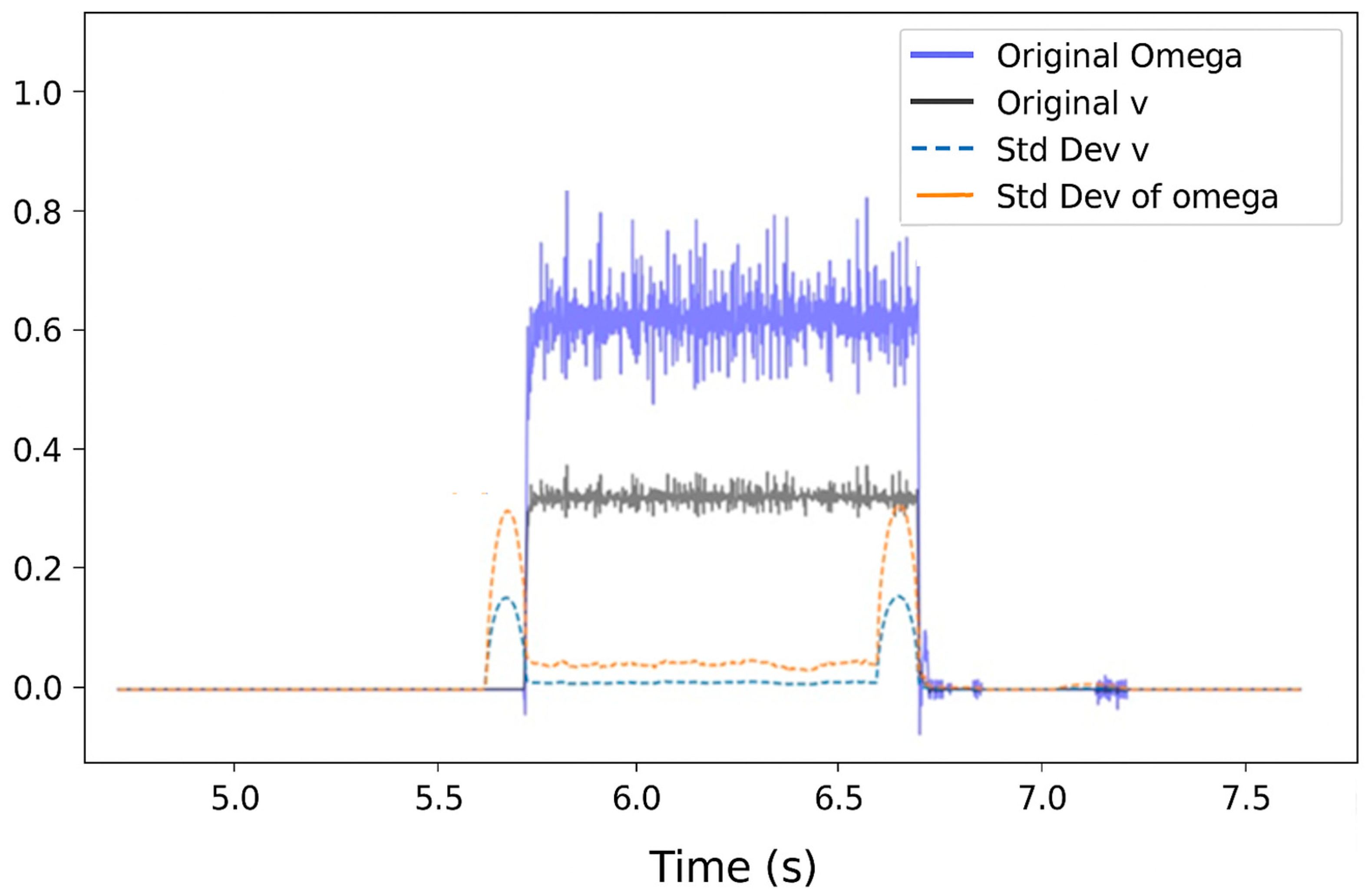Figure 2 shows the scatter deviation of the odometry data.

The calculated standard deviations are then appended to the original dataset, creating a new, extended dataset. This new dataset is saved in a separate CSV file.

• “Original Omega” shows the angular velocity of the robot as a function of time. When the robot turns left, the omega is positive, as indicated by the blue line in the graph. The changes in angular velocity are critical for the robot’s navigation system because they determine the robot’s orientation changes, including direction and speed.
• “Std Dev of Omega” (standard deviation) represents the variability of angular velocity over time. A low standard deviation indicates that the angular velocity is relatively consistent, while higher values suggest variability or instability. The orange dashed line on the graph highlights periods when the robot’s turning speed exhibited greater fluctuations.
• “Original v” shows the robot’s linear speed as a function of time. Linear speed is important for positioning the robot during straight-line movements. Maintaining a constant velocity is essential for predictable and accurate navigation, as shown in Figure 3.
• “Std Dev of v” (standard deviation) reflects the variability of linear velocity. If the robot is moving smoothly at a predefined speed, the standard deviation will remain low. Higher values indicate that the robot’s speed is variable, making precise tracking and stable operation more challenging.

To summarize, the calculation of the deviations in omega and v variance analyzes two distinct aspects of the robot’s motion. The deviation of omega variance reflects the stability and predictability of the robot’s turns, while the deviation of v variance reflects the smoothness and reliability of the linear motion. Both measurements are crucial for fine-tuning robot motion and improving navigation algorithms. A thorough analysis of these data can help system designers and operators optimize motion models and enhance overall robot performance.

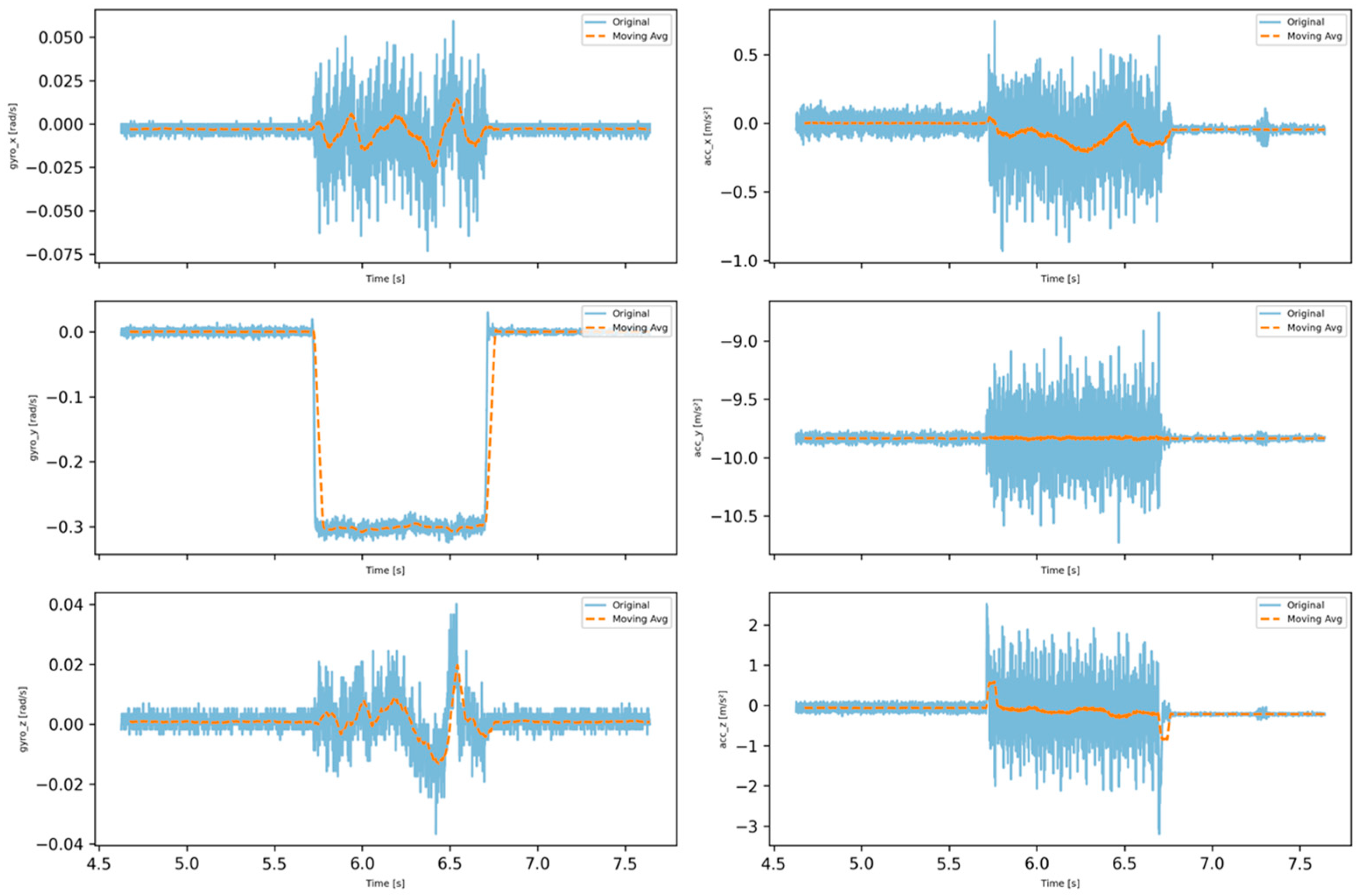
Overall, the stability or low variance levels observed in Gyro_x and Acc_x indicate that the robot maintained stable direction and velocity along the x-axis, which is a positive sign during the turning maneuver. In contrast, the high variance in Gyro_y and Acc_y suggests that the robot’s motion along the y-axis was more variable, which could imply inconsistent turning behavior. This variability may pose a potential issue from both a stability and motion control perspective. The observed changes in Gyro_y and Acc_y during the left turn were expected, as they are directly linked to the turning motion. Additionally, the variation in Gyro_z and Acc_z data indicates that the robot’s tilt changed during the maneuver.

Applying a moving average filter to the IMU and wheel-code data (Figure 4) offers significant benefits. This filter is an effective tool for reducing noise and minimizing short-term fluctuations while preserving the underlying trends in the data. The moving average filter works by averaging recent measurements from the dataset, which helps smooth out short-term changes and create a more consistent data series. This is particularly useful in robotics, where sensor data often contain random noise or sudden changes caused by the robot’s movements or environmental factors.

When the robot is navigating, the moving average filter helps smooth the data, providing a clearer picture of the true trends in its movements. This allows navigation algorithms to make more reliable decisions. By filtering out random fluctuations that could distort the evaluation of the robot’s motion, the moving average provides a more stable foundation for motion planning and fine-tuning motion control systems. The use of this filter enhances the robustness of the robot system against external disturbances, promotes more accurate and smoother movements, and ultimately contributes to improved robot performance and reliability.

The left turn in the IMU data of the robot is measured, in particular, by the gyro ‘gyro_y’ axis of the robot. A pop-out event in the ‘gyro_y’ graph, where the angular velocity value shows a sharp change, indicates a left turn. Since the measurement axes of the gyroscope are defined according to the robot’s own axis system, a positive or negative value along a given axis indicates the direction of rotation. If there is a large positive or negative offset on the ‘gyro_y’ axis, this may indicate that the robot has turned counter-clockwise (left) or clockwise (right) (Figure 5).

The usefulness of the moving average in this case is twofold: It helps to highlight the turning event by smoothing the data, and it helps to distinguish real motion from short-term noise. This smoothing can be particularly useful if we want to correctly identify and describe the turning motion in time, as it allows us to focus on the real motion, rather than the noisy data.

The formula for calculating the moving average of a time-series data Yt over a window of size k is:

$$M{A}_t={\displaystyle \frac{1}{k}}{\sum }_{i=0}^{k-1}{Y}_{t-i},$$

where MA_t is the moving average at time t, Y_t is the value of the time series at time t_t,k is the size of the moving average window, and i is the index within the window.

4.1. Correlation

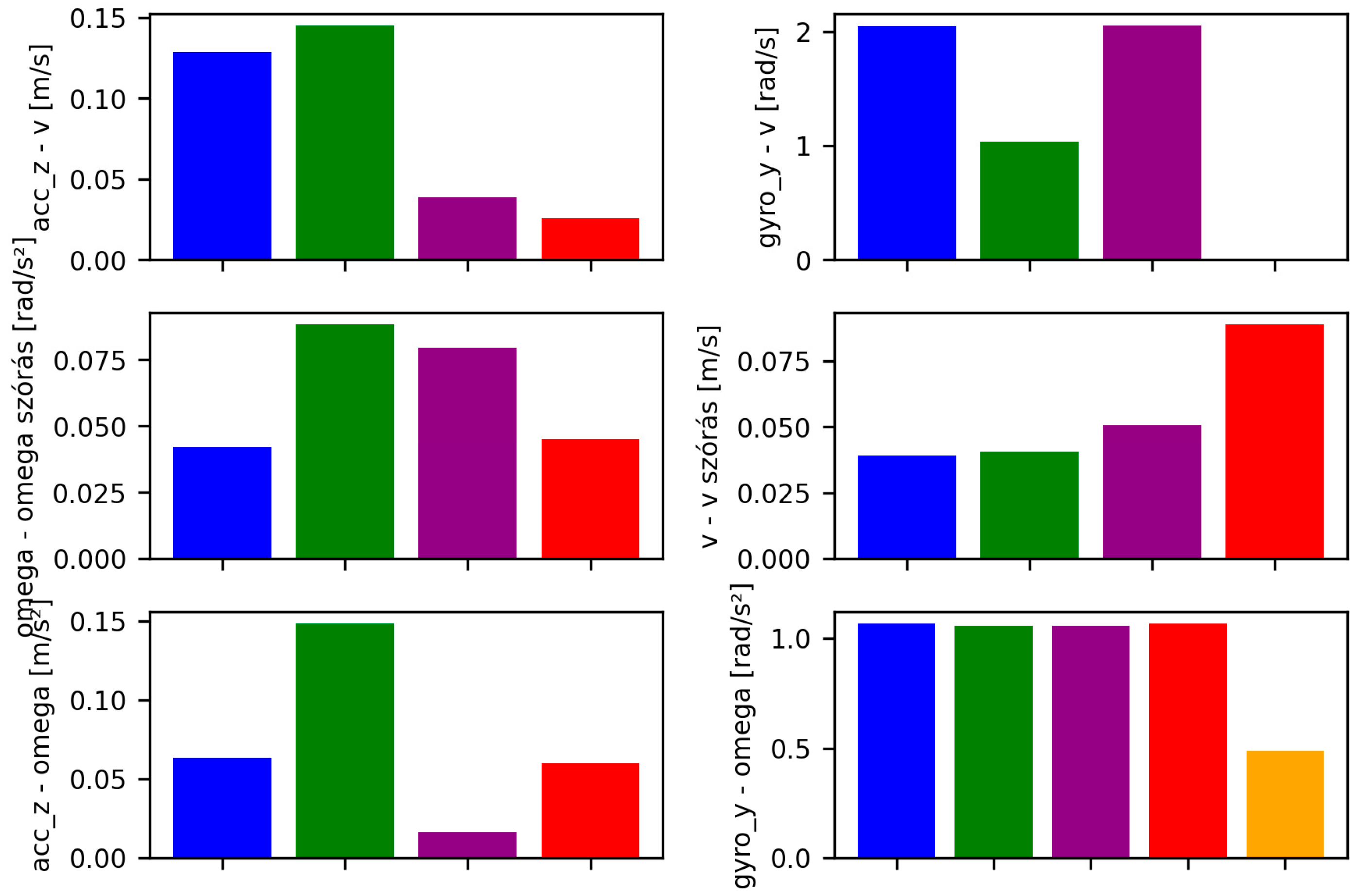
Correlation in the context of mobile robots can help identify the extent to which data from the robot’s sensors are interdependent. For instance, when measuring the robot’s motion and the changes in its environment, correlation can shed light on how data from individual sensors influence each other. This method is particularly useful in the development of a robot navigation system, as it helps to understand the relationship between data from various sensors and the robot’s movements and interactions with its environment. By using correlation, developers can better optimize the robot’s sensor system, thereby improving navigation accuracy and efficiency.

Correlation plays a crucial role in analyzing the PlatypOUs robot’s sensor data. Odometry data from the wheel encoders, which provides information on position and velocity, and IMU data, which measures acceleration and angular velocity, offer different types of motion-related information. Correlation can be employed to explore how these data sets are interconnected, aiding in the creation of a more accurate model of the robot’s motion and navigation. For example, if the velocity measured by the wheel encoders does not correlate well with the accelerations measured by the IMU, this may signal sensor errors or calibration issues (Figure 6).

The low correlation between acceleration and velocity during straight-line motion indicates that changes in velocity during this phase are less influenced by acceleration. This suggests that the robot’s velocity remains relatively stable during straight motion, with acceleration playing a smaller role in velocity changes. The observed low correlation could also be due to issues with sensor data, which are still under investigation.

In contrast, the higher correlation observed during turns suggests that acceleration has a greater impact on velocity changes in this phase. Notably, this relationship is even more pronounced during right turns, indicating that acceleration has a stronger influence on velocity in right turns compared to left turns.

These findings imply that the robot’s physical characteristics or sensor sensitivity may vary depending on the type of motion. The insights gained from data analysis can help identify and address potential sensor failures, ultimately improving the robot’s performance and reliability under different conditions.

The data analysis reveals minimal correlation between linear velocity and Z-axis acceleration during straight-line travel, suggesting that acceleration has little effect on velocity in this state. However, in turns, particularly right turns, the correlation between acceleration and velocity becomes stronger. A similar pattern is observed with angular velocity along the Y-axis and linear velocity. The variability of angular velocity is larger in right turns, which could reflect differences in motion dynamics or sensor accuracy. Additionally, the variance in linear velocity is greatest during straight travel and significantly smaller during stationary turns. In both cases, the highest correlation is observed during left turns in place, suggesting that the relationship between acceleration and angular velocity is strongest in this specific motion state.

In statistics, theoretical values are not available, and empirical correlation is therefore calculated as follows:

$$r_{X,Y}={\displaystyle \frac{\sum _{i=1}^n(X_i-\overline{X})(Y_i-\overline{Y})}{\left(n-1\right)s_X{s}_Y}}$$

Correlation can be calculated using statistical software. This can be found in the statistics/analyze menu. The software provides descriptive statistics, the value of the correlation coefficient (r), and the significance level (denoted by p/sig), and sometimes also the confidence interval.

4.2. Exponential Smoothing

The application of exponential filtering in the analysis of sensor data from mobile robots is highly effective for reducing noise and adapting to rapid environmental changes. This filter type is particularly well-suited for mobile robots with limited resources, as it is computationally efficient and easy to implement. Exponential filters help eliminate sensor-generated noise, ensuring stable robot navigation and effective interaction with the environment.

By assigning more weight to recent measurements, exponential filters allow robots to respond quickly to environmental changes, which is crucial for efficient operation in dynamic environments. Additionally, they help robots track long-term trends while filtering out short-term fluctuations.

Setting the α value correctly is crucial, as it determines the speed at which the filter reacts to new data relative to older data. The optimal value for α depends on factors such as the robot’s speed, environmental conditions, and the specific task at hand. This parameter is typically set through experimental or adaptive methods.

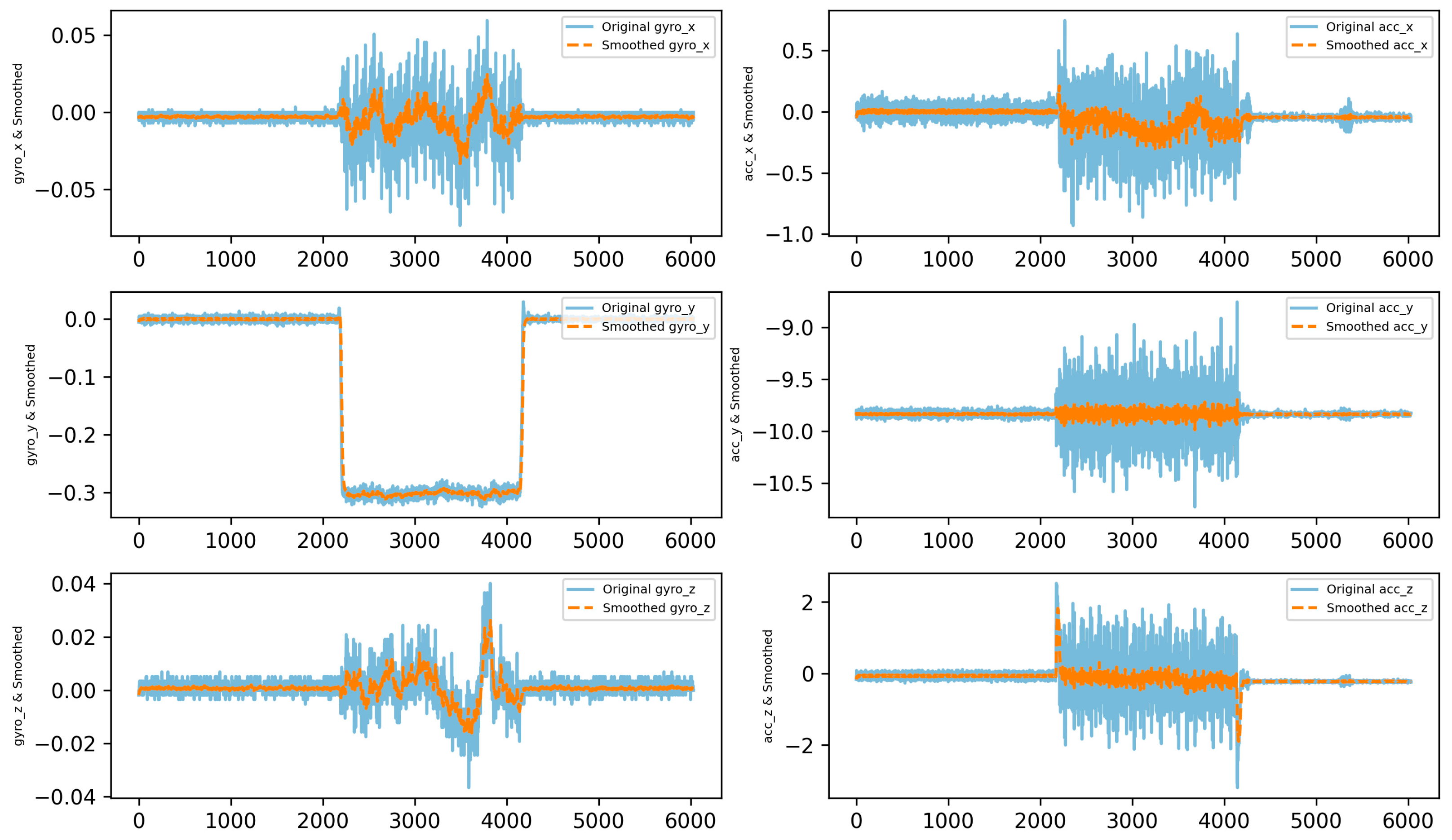
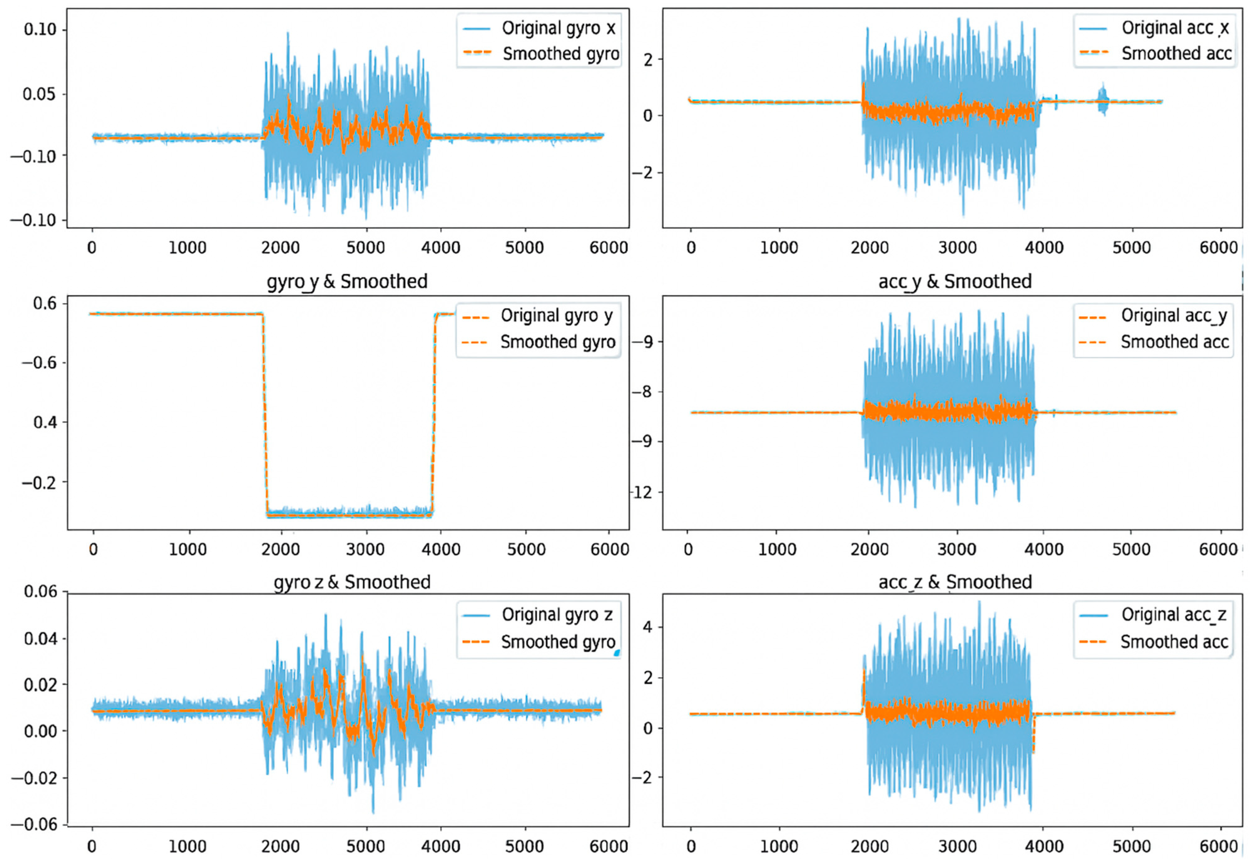
Exponential smoothing effectively reduces the noise in the gyroscope and accelerometer data, allowing for more accurate observation of the robot’s real-world motion. The rotation along the X-axis shows a stable trend, although with some outliers. Y-axis rotation was relatively stable with little noise. The angular velocity and acceleration along the Z-axis showed initial noise data, but became more stable after smoothing, reflecting the dynamics of the robot’s motion. The smoothed data help to more easily interpret the smooth trends and possible changes, which will facilitate more accurate navigation and environmental interactions (Figure 7).

Exponential smoothing effectively reduced noise in the gyroscope and accelerometer data, allowing the robot to detect and react more accurately to environmental changes, such as turning left. The smoothed data illustrate smoother and more easily interpretable trends, which helps the robot to navigate stably and perform environmental interactions more accurately. The use of a filter helps the robot’s control system to make more accurate decisions, as smoothed signals contain less random fluctuations.

However, it is important to carefully adjust the smoothing factor α to determine the optimal balance between noise reduction and real-time responsiveness, especially for dynamic maneuvers, such as turns.

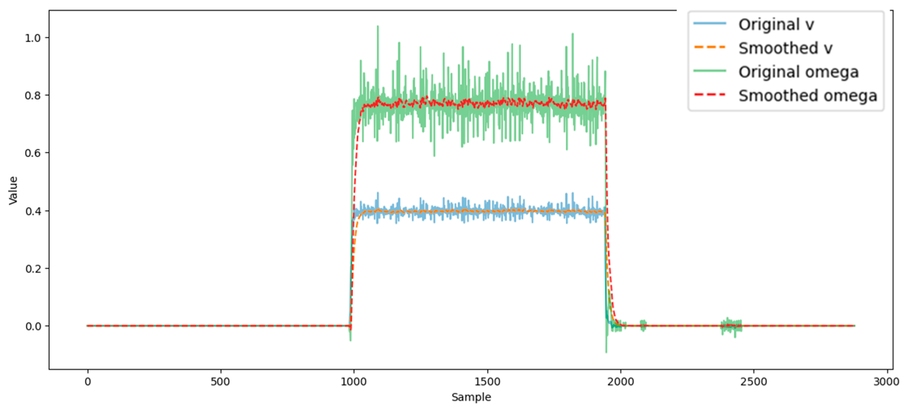
The “Original v” data show slight noise, but are stable, indicating steady progress. The smoothed linear velocity curve further reduces the noise, preserving the overall trend of the original data. Consistent altitude indicates a steady speed, suggesting stability during the turning maneuver (Figure 8).

The “Original omega” data shows significant noise and fluctuation, probably due to wheel encoder or measurement inaccuracies. The smoothed angular speed curve shows a sudden change, indicating the time of the left turn. After the turn, the omega value returns to near-zero, indicating that the robot has completed the turn and is moving in a straight line again.

The stability of the linear velocity during the turning maneuver suggests that the robot was able to maintain forward velocity during the turning maneuver, which may be a good indication of the efficiency of the robot’s propulsion and control system. The sharp change in the smoothed omega curve shows that the turning maneuver was dynamic, and the exponential smoothing effectively filters out noise, so that the time and duration of the actual turning maneuver can be easily identified. Taken together, these data indicate that the robot performed a controlled and smooth left turn. The simulations allow for a more accurate analysis of the odometry data and a better understanding of the robot’s motion.

The formula for exponential smoothing can be expressed as follows:

$$S_t=\alpha ·Y_t+(1-\alpha )·S_{t-1}$$

where St is the current smoothed value, Y_t is the current observed value, S_t−1 is the previous smoothed value, and α is the smoothing factor (a value between 0 and 1) that determines how much weight is given to the previous value when calculating the current value. The closer α is to 1, more weight is placed on the current value.

5. Discussion

The stability or low variance in Gyro_x and Acc_x indicates that the robot maintained its direction and velocity along the x-axis, which is a positive sign during turning maneuvers. In contrast, the high variance in Gyro_y and Acc_y suggests that the robot’s motion along the y-axis was more variable, which may indicate inconsistent turning behavior. This variability could pose a problem from a stability and motion control perspective. The changes in Gyro_y and Acc_y during the left turn were expected, as these data are directly related to the turning motion. Additionally, changes in Gyro_z and Acc_z data show that the robot’s tilt also changed during the maneuver.

In summary, the calculation of omega and v variance deviations analyzes two distinct aspects of robot motion. The omega variance deviation assesses the stability and predictability of the robot’s turns, while the v variance deviation examines the smoothness and reliability of the robot’s linear motion. Both measurements are essential for fine-tuning robot motion and developing navigation algorithms.

The moving average filter serves two key purposes in this context: first, it helps highlight the turning event by smoothing the data, and second, it helps distinguish real movement from short-term noise. This smoothing is particularly useful for accurately identifying and describing the turning motion over time, as it allows us to focus on the true motion rather than on noisy data.

The acceleration values along the acc_x and acc_y axes may also exhibit variations during the turn, but these variations are generally less characteristic than the gyroscope data. On the acc_z axis, the effect of gravity makes it less likely that the turn will be evident, unless the robot’s mass changes during the maneuver.

The moving average filter makes it easier to identify and analyze dynamic behaviors associated with a left turn, providing a clearer picture of the robot’s directional change. By using the moving average, we can see that the robot’s linear velocity remained relatively constant for most of the measurement period, while the angular velocity graph clearly indicates the time and duration of the turn. The smoothed moving average makes the robot’s motion easier to interpret, especially during turning maneuvers, where the original data may be distorted by significant noise and fluctuations.

Much of the system development originates from the experience of robotics and STEM education practices at Obuda University. Unlike standard robot visualization tools such as RViz, which focus on spatial representations without exposing raw sensor streams for analytical exploration, our proposed platform directly integrates data processing and visualization into the educational workflow. This allows learners to engage with statistical methods like moving average filtering, exponential smoothing, and correlation analysis, fostering a deeper understanding of robot dynamics and the influence of sensor noise. Compared to simulation tools like Gazebo or educational kits like LEGO Mindstorms, which abstract away sensor-level complexities, PlatypOUs emphasizes data transparency and equips students with practical skills in both robotics and data analysis. This dual focus on real-time data-driven decision-making and system debugging addresses a gap in current robotics education tools, aiming to enhance the learning experience in STEM.

6. Future Work

Arguably, the work is still ongoing, with significant potential for future development. To begin with, it is expected to extend our data pool by including numerous representative motion patterns—straight-line traversal and an approximation of a slalom-like path, repeated in numerous iterations.

Further developments could extend the research in several directions to gain a deeper understanding of robot motion and enable the application of adaptive non-linear control algorithms [33]. It is crucial to utilize various types and amounts of data for a more detailed analysis, which will help better understand different aspects of the robot’s movement and ultimately allow for the application of deep learning methods to the dataset [34].

Additionally, the introduction of new sensors, sensor fusion, and advanced filtering techniques—such as the integration of laser scanners and the latest versions of depth cameras (e.g., the Intel RealSense D555)—could enhance the robot’s ability to detect motion more accurately and improve its navigation capabilities [35]. Advances in material development, particularly in additive manufacturing, could lead to the creation of lightweight yet durable structures for the robot’s base, enabling the integration of more sensors [36].

Expanding the modalities and scope of the collected data would allow for an update to the data analysis window size, which is an interesting avenue for identifying the optimal setting. Furthermore, exploring different motion parameter configurations could offer new perspectives on navigational capabilities and stability. A comprehensive revision aimed at scalability and future integration into educational systems is also essential. In the proposed future assessment session, students shall indicate how much they agree with the above statements about their experience using the PlatypOUs robot and data analysis platform (including data processing and visualization tools) for analyzing their own robot-collected data (Figure 9). Certain modern robot system development frameworks, such as the IEEE’s Ethically Aligned Design principle (published as standard: IEEE 7007-2022) [37,38], could be applied to ensure ethical development and alignment with industry best practices. Overall, these innovative approaches could enable robots to operate more efficiently and accurately, offering new opportunities and advancements in the field of robotics.

7. Conclusions

In summary, the data analysis demonstrates that the robot maintained stability and consistent direction along the x-axis during the turning maneuver, reflecting effective control. However, variability in the Gyro_y and Acc_y data suggests some inconsistency in the robot’s motion along the y-axis, which could affect stability during left turns. Despite this, the variations in Gyro_y and Acc_y were expected, as they are directly related to the turning motion. Changes in the Gyro_z and Acc_z data indicate adjustments in the robot’s tilt during the maneuver.

The omega and v variance deviations provide valuable insights into turn stability and the smoothness of linear motion, which are crucial for refining motion control and developing navigation algorithms. The moving average filter serves a dual purpose: it highlights the turning event while filtering out short-term noise, facilitating the accurate identification of turning patterns. While acceleration data along the acc_x and acc_y axes exhibit some variation, this is less pronounced compared to the gyroscope data, with gravity largely influencing acc_z.

Overall, this analysis effectively describes the robot’s performance during a left turn, underscoring the importance of stability and predictability in turns, as well as smooth linear motion. The moving average filter helps differentiate real motion from noise, contributing to a deeper understanding that supports the optimization of motion control and navigation algorithms. Ultimately, these improvements enhance the robot’s performance and reliability.