Robotic Positioning Accuracy Enhancement via Memory Red Billed Blue Magpie Optimizer and Adaptive Momentum PSO Tuned Graph Neural Network

Abstract

Robotic positioning accuracy is critically affected by both geometric and non-geometric errors. To address this dual error issue comprehensively, this paper proposes a novel two-stage compensation framework. First, a Memory based red billed blue magpie optimizer (MRBMO) is employed to identify and compensate for geometric errors by optimizing the geometric parameters based on end-effector observations. This memory-guided evolutionary mechanism effectively enhances the convergence accuracy and stability of the geometric calibration process. Second, a tuned graph neural network (AMPSO-GNN) is developed to model and compensate for non-geometric errors, such as cable deformation, thermal drift, and control imperfections. The GNN architecture captures the topological structure of the robotic system, while the adaptive momentum PSO dynamically optimizes the network’s hyperparameters for improved generalization. Experimental results on a six-axis industrial robot demonstrate that the proposed method significantly reduces residual positioning errors, achieving higher accuracy compared to conventional calibration and compensation strategies. This dual-compensation approach offers a scalable and robust solution for precision-critical robotic applications.

1. Introduction

With the rapid advancement of industrial automation and intelligent manufacturing, robotic technology has been widely applied in the manufacturing industry and has become a critical productive tool. Industrial robots are extensively used in complex processes such as welding, assembly, grinding, and gluing due to their high positioning accuracy, excellent repeatability, and long-term operational stability [1]. In recent years, the concept of Human-Robot Collaboration (HRC) has emerged, further elevating the requirements for robotic motion accuracy. Especially in tasks involving collaborative operations and high-precision manufacturing, greater demands are being placed on robots’ positioning and trajectory control capabilities. Typically, robotic systems exhibit high repeatability, often reaching sub-millimeter or even micrometer-level precision, primarily governed by mechanical structural errors. However, their absolute positioning accuracy remains relatively low, often limited by the accuracy of kinematic models and system-level error sources. As a result, improving robots’ absolute positioning accuracy has become a key issue in enhancing task quality and advancing system intelligence. In terms of error sources, robot positioning errors can be broadly categorized into geometric error and non-geometric error. The former arises mainly from link parameters, installation deviations, and joint zero-offsets, which are closely related to kinematic modeling. To address geometric errors, kinematic calibration techniques are commonly employed, involving the optimization of Denavit–Hartenberg (DH) parameters or the construction of error compensation models to significantly enhance model fidelity and positioning accuracy [2]. However, kinematic calibration alone cannot fully eliminate positioning errors. In practical applications, non-geometric errors—such as joint backlash, elastic deformation, thermal expansion, load-induced disturbances, and drive friction–also play a critical role. These nonlinear and time varying errors are difficult to model and compensate using traditional methods, posing a major challenge to achieving high-precision robotic performance. To address this issue, recent research has increasingly focused on data-driven approaches and intelligent compensation mechanisms for modeling and mitigating non-geometric errors. Representative methods include neural networks, support vector regression, and fuzzy logic systems, which learn and approximate the mapping relationships from observed motion behavior [3]. These models enable real-time compensation during task execution, thereby enhancing overall motion accuracy and system stability. As such, hybrid modeling and optimization methods that integrate geometric calibration with non-geometric error compensation have emerged as a promising research direction for improving the positioning and control precision of robotic systems.

During geometric calibration, a model describing geometric errors in terms of the robot’s structural parameters is developed, and the deviations in these parameters are subsequently estimated. Geometric calibration commonly employs methods such as least squares estimation (LSE), Levenberg–Marquardt (LM), extended Kalman filter (EKF), and particle swarm optimization (PSO). Gao et al. [4] introduced an LSE approach to identify geometric parameter errors in articulated arm coordinate measuring machines. While the LSE method offers rapid convergence, it exhibits high sensitivity to measurement noise. Deng et al. [5] designed a Chebyshev interpolated Levenberg–Marquardt (CILM) algorithm to compensate for path deviations in a robotic smoothing system, thereby improving the absolute positioning accuracy. Deng et al. [6] developed an adaptive residual extended Kalman filter-based calibration method, combined with an improved butterfly optimization algorithm, to enhance the absolute positioning accuracy of robots. Chen et al. [7] developed an improved multi-objective PSO algorithm to construct optimal measurement configurations for drilling robot calibration, effectively enhancing kinematic parameter identification accuracy and end-effector positioning performance. Although the aforementioned learning-based algorithms are capable of performing robot calibration, their effectiveness significantly diminishes in the presence of non-geometric errors. Moreover, these methods often exhibit limitations such as slow convergence rates and reduced calibration accuracy, particularly when dealing with complex, nonlinear error sources [8]. Consequently, their application in high-precision robotic systems remains constrained.

In the context of non-geometric calibration, a model-independent strategy has been introduced to compensate for errors without relying on explicit system modeling. Cao et al. [9] proposed a robot calibration method based on an extended Kalman filter (EKF) and an artificial neural network optimized by the butterfly and flower pollination algorithm (ANN-BFPA) to improve the robot’s absolute pose accuracy. Kong et al. [10] proposed an online calibration method combining LSTM-EKF and neural networks to enhance the positioning accuracy of large, high-speed industrial robots under dynamic operating conditions. Maghami et al. [3] applied a two-step ANN–based calibration strategy to enhance both the absolute and relative positioning accuracy in a master-slave cooperative robot system. Chen et al. [11] proposed a positional error compensation method combining error similarity and RBF neural networks, which effectively improves the absolute positioning accuracy of industrial robots. The aforementioned studies highlight the potential of using data-driven neural networks to compensate for non-geometric errors in robotic manipulators. Nevertheless, these approaches predominantly rely on conventional multilayer perceptron (MLP) architectures, which are often insufficient for capturing the intricate and highly nonlinear characteristics of non-geometric errors. Due to their limited representational capacity, basic MLPs may struggle to model the dynamic and context-dependent error patterns arising from joint compliance, thermal effects, and sensor noise, thereby constraining the overall calibration performance in high-precision applications.

To systematically evaluate existing approaches for enhancing robotic positioning accuracy, both geometric calibration methods and non-geometric error compensation techniques must be considered. Geometric calibration primarily focuses on optimizing structural parameters through model-based identification, whereas non-geometric compensation addresses dynamic and time-varying disturbances using data-driven models.

Table 1. Comparative evaluation of existing geometric calibration approaches.

Approaches	Strengths	Weaknesses
Least squares [4]	The least squares algorithm with regularization improves numerical stability and is effective for identifying kinematic errors in over-constrained parallel kinematic mechanisms. It works well with linearized models and has been validated by both simulation and experiments.	This method is sensitive to outliers and depends on the accuracy of the model. It performs poorly for highly nonlinear systems and requires careful tuning of the regularization parameter.
Levenberg-Marquardt [5]	The LM algorithm offers fast convergence and improved numerical stability, making it suitable for solving nonlinear least squares problems in robotic calibration under noise and constraints.	Despite its efficiency, the LM algorithm is prone to truncation errors and may face difficulty in escaping local minima, especially when the initial guess is far from the true solution.
Filtering-based methods [6]	Filtering-based methods are widely used in robot calibration for their ability to handle dynamic, uncertain, and nonlinear environments. They enable accurate state and parameter estimation under noise by combining system models with measurement feedback. For example, EKF handles Gaussian noise with real-time efficiency, while PF is effective in non-Gaussian and highly nonlinear cases.	These methods rely heavily on accurate initial values and model assumptions. EKF may suffer from linearization (truncation) errors, and PF is sensitive to the prior distribution and can be computationally intensive.
Maximum Likelihood Estimation [8]	Maximum likelihood estimation offers strong convergence properties and high calibration accuracy. It is particularly effective for modeling complex kinematic errors and is more flexible than traditional least squares methods, with better adaptability to iterative optimization frameworks.	Maximum likelihood estimation requires an accurate system model and high-quality measurement data. It can be computationally intensive due to iterative parameter estimation, and its effectiveness may decline when the model structure is poorly defined or the data are noisy.
Evolutionary computation methods [7]	Evolutionary algorithms like GA, PSO, and DE are robust for nonlinear, multi-modal calibration problems. They do not require gradient information and have strong global search ability, making them effective under noisy or complex conditions.	These methods can be computationally expensive and slow to converge. Their performance depends on parameter tuning, and results may vary due to randomness, requiring multiple runs or post-validation.

provides a comparative analysis of representative geometric calibration methods, including least squares, LM, filtering-based techniques, maximum likelihood estimation, and evolutionary computation approaches. These methods vary in accuracy, convergence behavior, model dependence, and computational complexity. In contrast,

Table 2. Comparison of representative approaches for non-geometric error compensation.

Approaches	Advantages	Disadvantages
BP Neural Network [3,9,10]	BP neural networks are easy to implement and capable of approximating complex nonlinear mappings between joint states and non-geometric errors. Their simplicity and wide applicability make them a common baseline model in robotic error compensation.	They often suffer from slow convergence and are prone to getting stuck in local minima. Performance is sensitive to network structure and hyperparameter settings, limiting scalability for complex systems.
RBF Neural Network [11]	RBF networks train quickly and are highly effective for modeling localized error patterns due to their strong interpolation capabilities. They are suitable for smooth, low-dimensional compensation tasks.	Their performance depends heavily on the choice of centers and spread parameters. They are less effective in high-dimensional or highly dynamic environments and can struggle with generalization.
Residual Neural Network [14]	ResNet structures overcome vanishing gradients through skip connections, enabling deeper models to accurately learn complex nonlinear relationships. They are particularly effective for modeling high-dimensional, multi-source error data.	They require large datasets and greater computational resources. The increased architectural complexity makes them more difficult to train and tune in practical robotic systems.
Convolutional Neural Network [15]	CNNs are excellent at extracting spatial features from structured data such as thermal fields or deformation maps. They are effective for modeling spatially varying errors and capturing local patterns.	CNNs are not ideal for low-dimensional input data like joint angles. Training requires large datasets and computing power, and their use is limited in systems lacking image-like inputs.
Graph Neural Network [16]	GNNs can naturally model the topological and spatial relationships in robot kinematic chains, making them well-suited for capturing complex joint dependencies. They offer strong generalization across configurations.	GNNs are more difficult to design and implement due to the need for graph construction and message-passing mechanisms. Their application in industrial calibration is still emerging and lacks standardized practices.

presents a comparative evaluation of non-geometric compensation strategies, with a particular emphasis on neural network-based architectures. These include traditional BP and RBF networks, as well as more advanced frameworks such as ResNet, CNNs, and GNNs. Each method demonstrates unique advantages in modeling complex nonlinear errors, while also exhibiting limitations in data dependency, generalization ability, and computational cost. Notably, Mon [12,13] proposed neural network control methods integrating Tikhonov regularization and fuzzy PDC-based LQR strategies, which enhance network generalization and control robustness, and hold promising potential for application in robot error compensation scenarios. Together, the two tables provide a comprehensive overview of current techniques in robot calibration, highlighting the need for hybrid, adaptive approaches that integrate model-based and data-driven methods.

To overcome the limitations identified in the comparative analysis of existing geometric and non-geometric calibration methods (as summarized in Table 1 and Table 2), this study introduces a novel approach that integrates the MRBMO with a GNN, where the GNN is trained using an AMPSO algorithm, as shown in Figure 1. The proposed method is designed to effectively compensate for positioning errors in robots by leveraging the global optimization capability of MRBMO and the powerful representation learning of GNNs. The key contributions of this work can be summarized as follows:

(a)

A memory-enhanced RBMO algorithm is proposed to accurately identify geometric errors in robot kinematic calibration, improving absolute positioning accuracy.

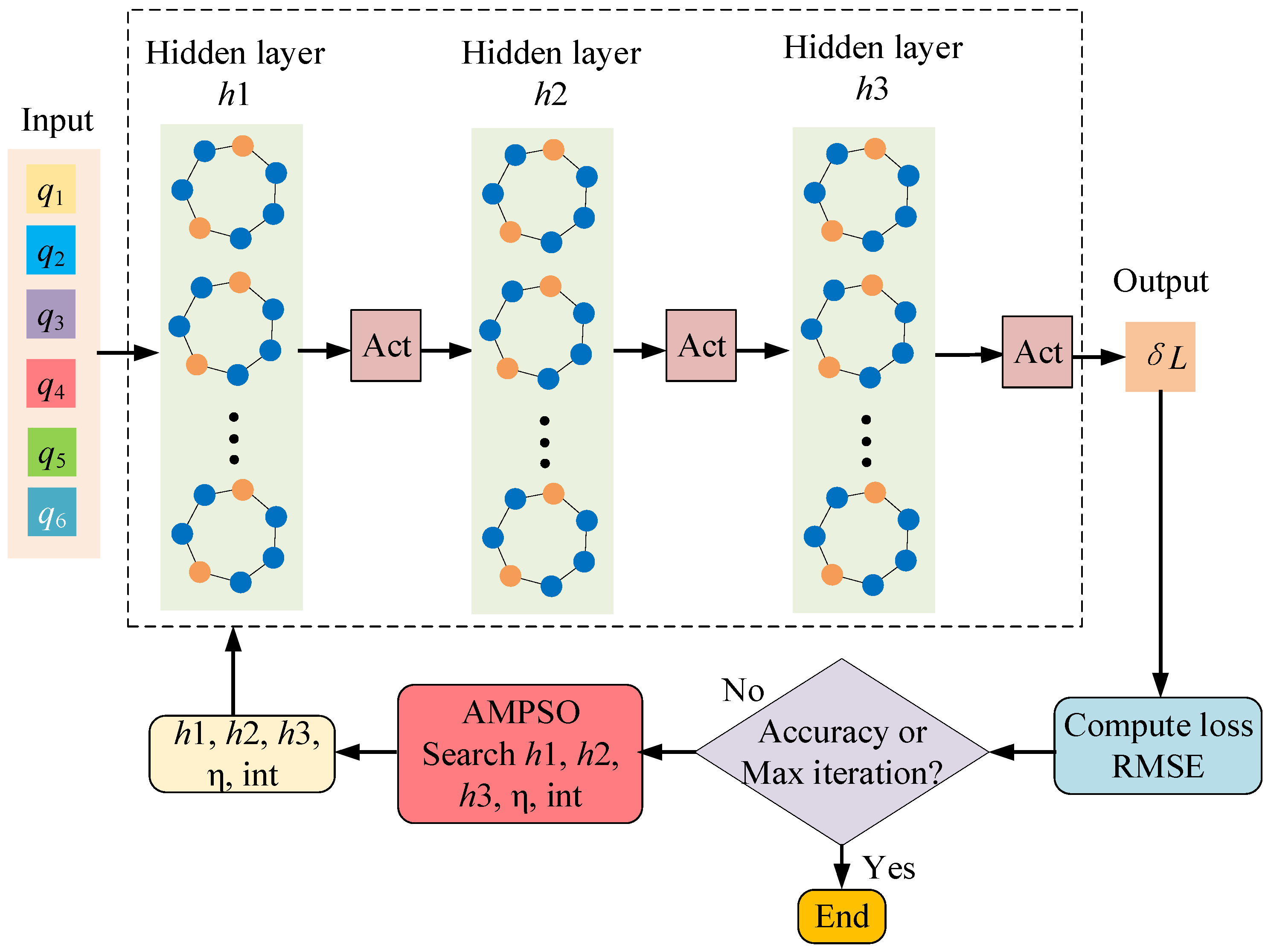
(b)

An adaptive momentum PSO is designed to optimize the GNN model, enabling effective compensation of nonlinear and time-varying non-geometric error.

The remainder of this paper is organized as follows. Section 2 introduces the robot kinematic model. Section 3 presents the MRBMO-based geometric error calibration method. Section 4 describes the AMPSO-GNN approach for non-geometric error compensation. Section 5 provides experimental validation, and Section 6 concludes the paper.

Figure 1. Schematic diagram of the robot calibration process.

Figure 1. Schematic diagram of the robot calibration process.

2. Kinematic Model of the Robot

As illustrated in Figure 2, the kinematic structure of the ABB IRB120 robot (ABB Ltd., Zurich, Switzerland) is modeled using the Denavit–Hartenberg (D-H) convention, which is widely regarded as the standard approach for establishing kinematic chains in industrial robots. Note that P_i represents the coordinate of the i-th measurement point (i = 1, 2, …, Num), and P_d denote the coordinate of the fixed end of the draw-wire sensor. P_r is the robot end position coordinates. By moving the robot end-effector to various P_i positions, the corresponding draw-wire lengths can be obtained. The Euclidean distance between P_i and P_d reflects the actual measured displacement and is used to evaluate the positioning error. Therefore, the calibration of the end-effector position is essentially reformulated as minimizing the error in the measured draw-wire length. This figure also presents the transformation matrix that describes the spatial relationship between the robot’s base frame and its end-effector frame, providing the mathematical foundation for motion analysis and calibration. Figure 2 depicts the measurement setup, which consists of the ABB IRB120 robot, a nylon traction wire, and a draw-wire displacement sensor. This system enables real-time measurement of end-effector displacements by recording the change in wire length as the end-effector moves within the robot’s workspace.

Due to the presence of both geometric and non-geometric error sources, along with measurement noise, the actual measured position of a robot’s end-effector often deviates from its intended or target position. This discrepancy can be mathematically represented by the measured position P_m of the end-effector as follows:

$$P_m=P_n+\Delta P_g+\Delta P_{ng}+\Delta P_{noise}$$

(1)

where P_m denotes the measured position, P_n is the target position, ΔP_g denotes geometric error, ΔP_ng stands for non-geometric error, and ΔP_noise represents the measurement noise.

The geometric errors of a robot are caused by inaccuracies in its geometric parameters and can be expressed as follows:

$$P_n+\Delta P_g=f_{forward}(g*)=f_{forward}(g+\delta g)$$

(2)

where f_forward(·) represents the forward kinematic function, g* denotes the true geometric parameter, g represents the nominal kinematic parameter, and δg corresponds to the geometric parameter error.

In robotic kinematic modeling, the Denavit–Hartenberg (D-H) convention is widely used to represent the kinematic parameters of the robot. This method systematically defines the geometric relationships between adjacent links and joints, and can be expressed as follows:

$$\begin{array}{c}{}_{i-1}{}^{i}T=Rot(X,{\alpha }_{i-1})Trans(X,a_{i-1})Rot(Z,{\theta }_i)Trans(Z,d_i)\\ =\left[\begin{array}{cccc}\cos {\theta }_i& -\cos {\alpha }_{i-1}\sin {\theta }_i& \sin {\alpha }_{i-1}\sin {\theta }_i& a_{i-1}\cos {\theta }_i\\ \sin {\theta }_i& \cos {\alpha }_{i-1}\cos {\theta }_i& -\sin {\alpha }_{i-1}\cos {\theta }_i& a_{i-1}\sin {\theta }_i\\ 0& \sin {\alpha }_{i-1}& \cos {\alpha }_{i-1}& d_i\\ 0& 0& 0& 1\end{array}\right]\end{array}$$

(3)

where α_i−1, a_i−1, d_i, and θ_i represent the link twist angle, link length, link offset, and joint angle, respectively, and ${}_{i-1}{}^{i}T$ denotes the transformation matrix from frame i − 1 to frame i. The operator Rot(⋅) indicates a rotation transformation, while Trans(⋅) denotes a translation transformation.

According to forward kinematics, the relationship between the end-effector pose of the robot and its joint variables can be expressed by the following transformation matrix:

$${}_0{}^{6}T={}_0{}^{1}T{}_1{}^{2}T{}_2{}^{3}T{}_3{}^{4}T{}_4{}^{5}T{}_5{}^{6}T=\left[\begin{array}{cccc}{n}_x& o_x& a_x& p_x\\ n_y& o_y& a_y& p_y\\ n_z& o_z& a_z& p_z\\ 0& 0& 0& 1\end{array}\right]=[\begin{array}{cc}{R}_r& P_r\\ 0& 1\end{array}]$$

(4)

where ${}_0{}^{6}T$ denotes the end-effector pose matrix; n_x, n_y, n_z, o_x, o_y, o_z, and a_x, a_y, a_z represent the rotational components of the pose matrix; p_x, p_y, p_z correspond to the elements of the position vector. R_r is the theoretical rotation matrix of the end-effector pose, and P_R is the corresponding position vector matrix.

Then f_forward can be expressed as:

$$f_{forward}=P_r{=}_0^{6}T((1:3),4)$$

(5)

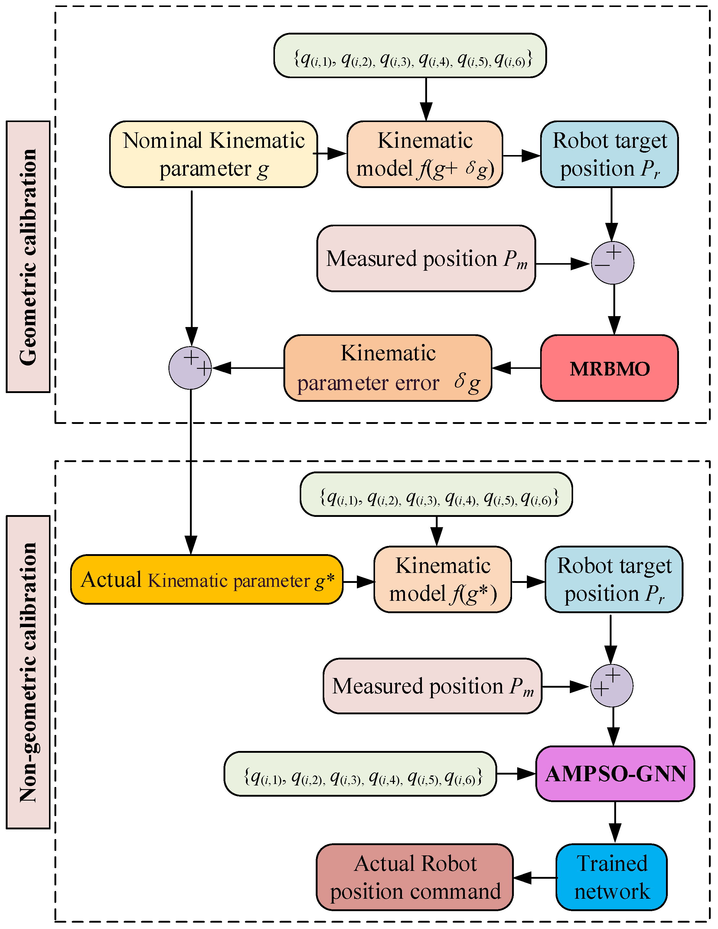
3. Robot Geometric Error Calibration

3.1. Loss Function

When using a draw-wire sensor for robot calibration, let L_i denote the measured cable length and L′_i represent the corresponding theoretical value computed based on the robot’s kinematic model. According to the fundamental principles of kinematic calibration, the following loss function can be formulated to optimize the Denavit–Hartenberg (D-H) parameters.

$$f(x)=\min {\displaystyle \frac{1}{n}}{\displaystyle \sum _{i=1}^n{‖L_i-L_i^{\prime }‖}_2}=\min {\displaystyle \frac{1}{n}}{\displaystyle \sum _{i=1}^n{‖L_i-{‖f_{forward}(g+x)-P_d‖}_2‖}_2}$$

(6)

where f(x) is the loss function with respect to the geometric parameter error vector x(δg), and the goal is to optimize x to minimize the positioning error.

3.2. Red Billed Blue Magpie Optimizer

The Red-billed Blue Magpie Optimizer (RBMO), introduced by Shengwei Fu et al. in May 2024 [17], is a swarm intelligence algorithm inspired by the foraging behavior of red-billed blue magpies, which includes stages such as exploration, prey capture, and food caching.

Like other algorithms, RBMO begins with random initialization of the population.

$$x(i,j)=lb+(ub-lb)\times rand$$

(7)

where x(i,j) represents the value of the j-th dimension of the i-th individual in the population, ub and lb denote the upper and lower limits of the search space, respectively, and Rand refers to a uniformly distributed random number in the range [0, 1].

Red-billed blue magpies exhibit flexible foraging behavior by operating either in small groups (2–5 individuals) or larger clusters (10 or more), adapting their strategies to environmental conditions and food availability to enhance search efficiency. In the RBMO algorithm, this behavior is modeled using different update mechanisms: Equation (8) governs the position update in small-group search, while Equation (9) applies to cluster-based foraging.

$$x_{k+1}(i,:)=x_k(i,:)+({\displaystyle \frac{1}{p}}\times {\displaystyle \sum _{m=1}^p{x}_k(m,:)}-x_k(rs,:))\cdot rand$$

(8)

$$x_{k+1}(i,:)=x_k(i,:)+({\displaystyle \frac{1}{q}}\times {\displaystyle \sum _{m=1}^q{x}_k(m,:)}-x_k(rs,:))\cdot rand$$

(9)

where x_k(i,:) denotes the position vector of the i-th individual in the k-th iteration, and x_k+1(i,:) is its updated position in the next iteration. x_k(m,:) represents the position of the m-th individual randomly selected from the population, and x_k(rs,:) denotes the position of a randomly selected reference individual used for guidance. The parameters p and q refer to the number of individuals randomly selected to form a small group and a large cluster, respectively, reflecting different foraging behaviors of red-billed blue magpies. The variable rand is a uniformly distributed random number in the interval [0, 1], which introduces stochastic perturbation and helps maintain population diversity.

Red-billed blue magpies demonstrate remarkable hunting skill and cooperative behavior during prey capture, employing tactics such as pecking, leaping, or aerial pursuit. In the RBMO model, small groups primarily focus on capturing smaller prey, modeled by Equation (10), while larger clusters aim at larger targets, as described by Equation (11).

$$x_{k+1}(i,:)=x_k(food,:)+CF*({\displaystyle \frac{1}{p}}\times {\displaystyle \sum _{m=1}^p{x}_k(m,:)}-x_k(i,:))\cdot randn$$

(10)

$$x_{k+1}(i,:)=x_k(food,:)+CF*({\displaystyle \frac{1}{q}}\times {\displaystyle \sum _{m=1}^q{x}_k(m,:)}-x_k(i,:))\cdot randn$$

(11)

where x_k(food,:) denotes the estimated position of the food source at the k iteration. The coefficient CF is a time-varying control factor defined as CF = (1 − k/K)^(2k/K), where k is the current iteration and K is the maximum number of iterations. randn is a randomly generated number following a standard normal distribution with a mean of 0 and a standard deviation of 1.

To foraging and attacking prey, red-billed blue magpies exhibit food caching behavior by storing surplus resources in concealed locations for future use. This strategy ensures a stable food supply during scarcity and is mathematically represented by Equation (12).

$$x_{k+1}(i,:)=\left\{\begin{array}{ll}{x}_k(i,:)& if fitnes{s}_{oid}(i)>fitnes{s}_{new}(i)\hspace{1em}\\ x_{k+1}(i,:)& \hspace{1em}\hspace{1em}else\end{array}\right.$$

(12)

where fitness_old(i) and fitness_new(i) denote the fitness values of the i-th red-billed blue magpie before and after its position is updated, respectively.

The RBMO algorithm exhibits an effective search mechanism and demonstrates solid overall performance. However, it still presents several limitations. Although RBMO performs well on specific types of problems, its current design may lack adaptability across a broader range of problem domains. Additionally, when applied to complex optimization tasks, scalability issues may emerge. The algorithm’s high computational burden—particularly in high-dimensional or large-scale settings—stems from the extensive number of iterations needed to achieve convergence, which may hinder its practicality in real-world applications where efficiency is critical.

3.3. Memory Based Red Billed Blue Magpie Optimizer

To further enhance the search accuracy and convergence stability of the original RBMO, this paper proposes an improved variant called the Memory-based Red-billed Blue Magpie Optimizer (MRBMO). The core idea of MRBMO is to incorporate individual-level memory guidance into the position update process, inspired by the concept of “personal best” in swarm intelligence.

In MRBMO, each red-billed blue magpie maintains a record of its historically best position, denoted as Pbest(i,:). During both the foraging and prey attack phases, this personal memory is used to guide the search direction, improving the balance between exploration and exploitation. Specifically, the update rule in the foraging phase is modified as:

$$x_{k+1}(i,:)=x_k(i,:)+dir\cdot rand+0.3\cdot (Pbest(i,:)-x_k(i,:))$$

(13)

where dir represents the directional vector based on group behavior, and the memory term pulls the individual towards its historical best. Similarly, during the prey attack stage, the update is reformulated as:

$$\begin{array}{l}{x}_{k+1}(i,:)=x_k(food,:)+CF\cdot (group\_mean-x_k(i,:))\cdot randn\\ \begin{array}{ccc}\hspace{1em}& \hspace{1em}& \hspace{1em}\end{array}+0.3\cdot (Pbest(i,:)-x_k(i,:))\end{array}$$

(14)

where group_mean is chosen based on a probabilistic switch. With probability ε, it is set to the mean position of a small randomly selected group ($X_{mean}^p$, and with probability 1 − ε, it is set to the mean position of a larger cluster ($X_{mean}^q$). This mechanism allows the algorithm to balance between local exploration and global convergence.

This memory-guided strategy helps preserve useful information from prior iterations and improves global search capability. The fitness of each individual is continuously monitored, and the personal best is updated whenever a better solution is found. This mechanism ensures that MRBMO avoids premature convergence while accelerating the optimization process.

Algorithm 1 outlines the pseudocode of the proposed MRBMO algorithm, which is employed for the identification of geometric parameters in robots.

Algorithm 1: MRBMO-GPI
Input: x0, {q(i,1), q(i,2), q(i,3), q(i,4), q(i,5), q(i,6)}, {L1, L2, L3, L4, L5, L6} Objective function f(⋅),    Search space boundaries Xmin, Xmax,    Population size N, maximum iteration K, k = 1
1.	Initialize population X∈RN×D with random values with in [Xmin, Xmax]
2.	Set Pbest←X, Pbest_fit(i)←∞ for all i
3.	Evaluate fitness of each individual f(x(i,:)), update Pbest(i,:) and global best xfood
4.	while k ≤ K do
5.	for i = 1 to N
6.	$\hspace{1em}\hspace{1em}\hspace{1em}\mathrm{Select} \mathrm{a} \mathrm{random} \mathrm{group} \mathrm{size} p\in [2, 5], \mathrm{compute} X_{mean}^p$
7.	$\hspace{1em}\hspace{1em}\hspace{1em}\mathrm{Select} \mathrm{a} \mathrm{larger} \mathrm{group} q\in [10, N], \mathrm{compute} X_{mean}^q$
8.	Select a random reference rs ∈ [1, N]
9.	if rand < ϵ
10.	$\hspace{1em}\hspace{1em}\hspace{1em}\hspace{1em}\mathrm{dir}=X_{mean}^p$$-x(rs,:), \mathrm{group}\mathrm{mean}=X_{mean}^p$
11.	else
12.	$\hspace{1em}\hspace{1em}\hspace{1em}\hspace{1em}\mathrm{dir}=X_{mean}^q$$-x(rs,:), \mathrm{group}\mathrm{mean}=X_{mean}^q$
13.	end if
14.	Update position: xk+1(i,:) = xk(i,:) + dir⋅rand + 0.3⋅(Pbest(i,:) − xk(i,:))
15.	Apply boundary check
16.	Evaluate new fitness, update Pbest(i,:) if improved
17.	Update global best xfood if improved
18.	end for
19.	Compute control factor: CF = (1 − k/K)(2k/K)
20.	for i = 1 to N
21.	Update with memory-guided prey attack:      xk+1(i,:)= xfood + CF⋅(group_mean − xk(i,:))⋅randn + 0.3⋅(Pbest(i,:) − xk(i,:))
22.	Apply boundary check
23.	Evaluate and update Pbest and xfood
24.	end for
25.	Increment iteration k = k + 1
26.	end while
	Return δg←xfood, ΔP←f(xfood)

4. Nongeometric Calibration

In addition to geometric deviations, the positioning accuracy of industrial robots is significantly influenced by nongeometric factors, such as cable interference, joint friction, mechanical backlash, and temperature drift. To effectively compensate for these errors, a data-driven nonlinear model is constructed using Graph Neural Networks (GNNs) [18], which maps the robot’s joint angles to a predicted position error, as shown in Figure 3.

The joint angles are taken as inputs and the drawstring length error as the output, with the objective of constructing a high-precision nonlinear mapping function to predict error distributions under different postures, thereby enabling effective modeling and compensation of non-geometric errors.

$$\widehat{y}=f_{GNN}(q;\theta )$$

(15)

where q denotes the robot’s joint angles q = [q₁, q₂,…,q₆]^T ∈ ℜ⁶, and $\widehat{y}$ is the GNN model prediction with network parameters θ = {W,b}. The objective is to learn the function f_GNN such that the output $\widehat{y}$ approximates the true nongeometric error y.

The six robot joints are represented as nodes in an undirected chain graph G = (V, E), where V denotes the set of nodes, each carrying a feature vector such as the joint angle, and E represents the set of edges that define adjacency relationships between nodes, which are used for message passing among neighbors during the GNN propagation process. The adjacency matrix A ∈ R^6×6 is defined as:

$$A_{ij}=\left\{\begin{array}{l}1,if\left|i-j\right|=1\\ 0,otherwise\end{array}\right.$$

(16)

The normalized adjacency matrix is:

$$A_{norm}=D^{-1}A,where\begin{array}{cc}{D}_{ii}={\displaystyle \sum _{j=1}^n{A}_{ij}}& \hspace{1em}\end{array}$$

(17)

where D is the degree matrix, which is a diagonal matrix. Specifically, D_ii represents the degree of node i, that is, the number of nodes it is connected to.

Assume a GNN with HL hidden layers. Given an input feature vector x ∈ R^6×1, the forward propagation equations are defined as:

$$\left\{\begin{array}{l}{H}^{(0)}=x\\ z^{(h+1)}=A_{norm}{H}^{(h)}\cdot W^{(h)}+b^{(h)},h=0,1,\dots ,HL-1\\ H^{(h+1)}=\sigma (z^{(h+1)})\end{array}\right.$$

(18)

where W(h) and b(h) are the weight and bias matrices of layer l, and σ(·) is the activation function (ReLU, LeakyReLU, or Tanh).

The final scalar output is computed by summing node embeddings:

$$\widehat{y}={\displaystyle \sum _{i=1}^6{H}_i^{(HL)}}$$

(19)

The network is trained to minimize the normalized mean squared error (MSE) loss:

$$𝓛(\theta )={\displaystyle \frac{1}{N}}{\displaystyle \sum _{i=1}^N{({\widehat{y}}_i-y_i)}^2}$$

(20)

where 𝓛(θ) is the training loss function.

Adam optimizer is used for parameter updates:

$$\left\{\begin{array}{l}{m}_t={\beta }_1{m}_{t-1}+(1-{\beta }_1){\nabla }_{\theta }𝓛\\ v_t={\beta }_2{v}_{t-1}+(1-{\beta }_2){({\nabla }_{\theta }𝓛)}^2\\ {\widehat{m}}_t={\displaystyle \frac{m_t}{1-{\beta }_1^t}},{\widehat{v}}_t={\displaystyle \frac{v_t}{1-{\beta }_2^t}}\\ {\theta }_t={\theta }_{t-1}-\eta \cdot {\displaystyle \frac{{\widehat{m}}_t}{\sqrt{{\widehat{v}}_t}+ϵ}}\end{array}\right.$$

(21)

where m_t denotes first moment estimate (mean of gradients), β₁ represents exponential decay rate for the first moment (typical value: 0.9), ∇_θ𝓛 stands for the gradient of the loss function with respect to the model parameters θ, v_t is second moment estimate (uncentered variance of gradients), β₂ denotes exponential decay rate for the second moment (typical value: 0.999), ${\widehat{m}}_t$ is bias-corrected first moment estimate, ${\widehat{v}}_t$ represents bias-corrected second moment estimate, θ_t is model parameters at iteration t, η is learning rate (step size), and є stands for small constant to prevent division by zero (e.g., 10⁻⁸).

To optimize the GNN’s structural parameters and learning rate, an AMPSO algorithm is employed.

Each particle encodes a candidate hyperparameter vector:

$$x=[h_1,h_2,h_3,\eta ,a,i]\in R^6$$

(22)

where h₁, h₂, h₃ are numbers of neurons in each hidden layer, respectively. η denotes learning rate, a represents activation function index (1 = ReLU, 2 = LeakyReLU, 3 = Tanh), and i stands for initialization method index (1 = Normal, 2 = Xavier, 3 = He).

In the AMPSO context, each particle encodes a candidate solution, and its fitness is evaluated via the objective function defined by the RMSE of the GNN model.

To update particles in the AMPSO framework, an adaptive momentum-driven velocity formulation is applied. The update process is governed by the following equations.

The inertia weight w^t, which controls the influence of previous velocities on the current velocity, is linearly decreased over iterations to balance global exploration and local exploitation:

$$w^t=w_{\max }-(w_{\max }-w_{\min })\cdot {\displaystyle \frac{t}{T}}$$

(23)

where w_max and w_min are the upper and lower bounds of inertia weight, respectively, t is the current iteration, and T is the total number of iterations.

The momentum coefficient m^t is dynamically adjusted based on the velocity dispersion of the particle population. This coefficient determines how much of the previous velocity $v_i^t$ is preserved when computing the new velocity. It is computed as:

$$\begin{array}{l}{\gamma }_v^t={\displaystyle \frac{1}{N}}{\displaystyle \sum _{i=1}^N‖v_i^t-{\overline{v}}^t‖},{\overline{v}}^t={\displaystyle \frac{1}{N}}{\displaystyle \sum _{i=1}^N{v}_i^t}\\ m^t=m_{\min }+(m_{\max }-m_{\min })\cdot \exp (-\lambda \cdot {\displaystyle \frac{{\gamma }_v^t}{{\gamma }_v^0+\zeta }})\end{array}$$

(24)

where $\overline{v_t}$ is the mean velocity of the population, and ${\gamma }_v^0$ and ${\gamma }_v^t$ are the initial velocity dispersion and velocity dispersion of the swarm at iteration t, respectively. λ is a decay control parameter, and ζ is a small positive constant to ensure numerical stability.

The velocity of the i-th particle at iteration t + 1, denoted $v_i^{t+1}$, is updated as:

$$\left\{\begin{array}{l}{v}_i^{t+1}=w^t\cdot [m^t\cdot v_i^t+c_1\cdot r_1\cdot (p_i^t-x_i^t)+c_2\cdot r_2\cdot (g^t-x_i^t)]\\ x_i^{t+1}=x_i^t+v_i^{t+1}\end{array}\right.$$

(25)

where $x_i^t$ and $x_i^{t+1}$ are iteration t and iteration t + 1 (i.e., hyperparameter vector) of particle i, respectively. ${{\displaystyle p}}_i^t$ is its personal best position so far, g^t is the global best found by the swarm, c₁ and c₂ are cognitive and social learning factors, respectively, and r₁, r₂∼U(0,1)^D are element-wise random vectors.

Each updated particle $x_i^{t+1}$ is evaluated by training a GNN with the corresponding hyperparameters and calculating the fitness using the root mean squared error (RMSE) on the testing set:

$$f_{rmse}(x_i^{t+1})=\sqrt{{\displaystyle \frac{1}{N}}{\displaystyle \sum _{j=1}^N{({\widehat{y}}_i-y_i)}^2}}$$

(26)

where ${\widehat{y}}_i$ and y_i are the predicted and true values of the j-th sample, respectively.

Then, personal and global best positions are updated if improvements are found:

$$p_i^{t+1}=\left\{\begin{array}{l}{x}_i^{t+1},if\begin{array}{cc}{f}_{rmse}(x_i^{t+1})<f_{rmse}(p_i^t)& \hspace{1em}\end{array}\\ p_i^t,\begin{array}{c}\hspace{1em} otherwise\end{array}\end{array}\right.$$

(27)

$$g^{t+1}=\arg \underset{i}{\min } f_{rmse}(p_i^{t+1})$$

(28)

In summary, the proposed AMPSO framework enhances the standard particle swarm optimization by introducing an adaptive momentum coefficient that dynamically responds to the velocity dispersion of the swarm. This mechanism enables the optimizer to better balance exploration and exploitation throughout the optimization process. The integration of time-decaying inertia weight and feedback-guided momentum improves convergence stability and search adaptiveness, especially in high-dimensional hyperparameter spaces such as those in deep graph neural network architectures. The encoded particle structure allows efficient tuning of architectural and training parameters, leading to improved GNN performance in modeling robotic nongeometric errors. The complete optimization process is summarized in Algorithm 2, where the adaptive momentum-guided hyperparameter search is embedded within the GNN training pipeline for nongeometric parameter identification.

Algorithm 2: AMPSO-GNN-NGPI
Input: Training data {qtrain, δLtrain}and testing data {qtest, δLtest}
1.	Initialize Population size N, particle dimension D = 6
2.	Maximum iterations T
3.	PSO parameters: wmax, wmin, c1, c2;
4.	Momentum parameters: mmax, mmin, λ, ζ
5.	Initialize X0 = Xmin + (Xmax − Xmin)·rand(N,D); V0 = Vmin + (Vmax − Vmin)·rand(N,D)
6.	For i = 1 to N
7.	$\hspace{1em}\hspace{1em}\hspace{1em}\mathrm{Decode} x_i^0$→(h1, h2, h3, η, act, init)
8.	Construct a fGNN
9.	$\hspace{1em}\hspace{1em}\hspace{1em}\mathrm{Train} \mathrm{the} \mathrm{GNN} \mathrm{on} 𝒟\_\mathrm{train} \mathrm{and} \mathrm{compute} \mathrm{prediction} \mathrm{error} \mathrm{on} 𝒟\_\mathrm{test}$ $\hspace{1em}\hspace{1em}\hspace{1em}\mathrm{Compute} {\widehat{y}}_{\mathrm{train}}$ = fGNN(qtrain, θ), ytest = fGNN(qtest, θ)
10.	$\hspace{1em}\hspace{1em}\hspace{1em}\mathrm{Compute} f_{\mathrm{rmse}}(x_i^0$)
11.	$\hspace{1em}\hspace{1em}\hspace{1em}\mathrm{Set} \mathrm{personal} \mathrm{best} p_i\leftarrow x_i^0$
12.	$\hspace{1em}\hspace{1em}\hspace{1em}\mathrm{If} f_{\mathrm{rmse}}(x_i^0$$) < f_{\mathrm{rmse}}(g), \mathrm{then} \mathrm{update} \mathrm{global} \mathrm{best} g\leftarrow x_i^0$
13.	end for
14.	$\mathrm{Compute} \mathrm{initial} \mathrm{velocity} \mathrm{dispersion} {\gamma }_v^0$$\leftarrow \mathrm{std}\left(\right\{v_i^0$})
15.	For t = 1 to T
16.	Compute wᵗ = wmax − (wmax − wmin) × (t/T)
17.	$\hspace{1em}\hspace{1em}\hspace{1em}\hspace{1em}\hspace{1em}\hspace{1em}\hspace{1em}{\gamma }_v^t$$=\mathrm{std}\left(\right\{v_i^t$})
18.	$\hspace{1em}\hspace{1em}\hspace{1em}\hspace{1em}\hspace{1em}\hspace{1em}\hspace{1em}{m}^t=m_{\min }+(m_{\max }-m_{\min }) \times \exp (-\lambda \times {\gamma }_v^t$$/({\gamma }_v^0$ + ζ))
19.	For i = 1 to N
20.	$\hspace{1em}\hspace{1em}\hspace{1em} \mathrm{Update} \mathrm{velocity}: v_i^{t+1}$$=w \times [ m^t+c_1·\mathrm{rand}·(p_i-x_i^t$$) + c_2·\mathrm{rand}·(g-x_i^t$)]
21.	$\hspace{1em}\hspace{1em}\hspace{1em} \mathrm{Update} \mathrm{position}: x_i^{t+1}$$=x_i^t$$+ v_i^{t+1}$
22.	$\hspace{1em}\hspace{1em}\hspace{1em}\hspace{1em}\mathrm{Clamp} v_i^{t+1}$$\in [v_{\min },v_{\max }], x_i^{t+1}$ ∈ [xmin, xmax]
23.	$\hspace{1em}\hspace{1em}\hspace{1em}\hspace{1em}\mathrm{Decode} x_i^{t+1}$→(h1, h2, h3, η, act, init)
24.	Build and train GNN with decoded structure on {qtrain, δLtrain}
25.	$\hspace{1em}\hspace{1em}\hspace{1em}\hspace{1em}\mathrm{Compute} \mathrm{RMSE} \mathrm{on} \{q_{\mathrm{test}}, L_{\mathrm{test}}\} \mathrm{as} \mathrm{fitness} f_{\mathrm{rmse}}(x_i^{t+1}$)
26.	$\hspace{1em}\hspace{1em}\hspace{1em}\hspace{1em}\mathrm{If} f_{\mathrm{rmse}}(x_i^{t+1}$$) < f_{\mathrm{rmse}}(p_i), \mathrm{then} \mathrm{update} p_i\leftarrow x_i^{t+1}$
27.	If frmse (pᵢ) < frmsef(g), then update g←pᵢ
28.	end for
29.	end for
30.	Return optimal solution g* = g and corresponding fitness frmse(g*)

5. Evaluation Results and Comparative Analysis

5.1. Implementation Details

Datasets: The dataset utilized in this study was acquired from an ABB IRB120 industrial robotic platform. It comprises a total of 1000 data samples, with each sample consisting of six joint angle values corresponding to the robot’s articulated structure, along with the measured cable length associated with that specific configuration. Each sample within the dataset comprises six joint angles and the corresponding measured distance between the robot’s end-effector and a fixed target point. To mitigate sampling bias and ensure statistical robustness, 200 samples are randomly drawn using a uniform distribution to form one testing case. This sampling process is repeated ten times, resulting in ten distinct data scenarios. For each case, the dataset is divided into 80% for training and 20% for testing, which serves as the basis for model evaluation. The performance of each model is assessed across all ten cases, and the mean and standard deviation of the results are computed to ensure objective reporting. During training, the optimization process for each model is terminated either when the improvement of the objective function between two successive iterations falls below 10⁻³, or when the number of iterations reaches a maximum of 50. Figure 4 shows the 3D distribution of the selected calibration and validation points in the workspace, demonstrating that the sampled data adequately cover the entire reachable area of the ABB IRB120 robot.

To promote research reproducibility and ensure openness, the dataset used in this study—accompanied by comprehensive documentation—has been publicly released. It is accessible at https://github.com/Lizhibing1490183152/RobotCali (accessed on 1 August 2022). This publicly available resource serves as a reliable benchmark for evaluating calibration algorithms and advancing further research in the field of robot calibration.

Figure 4. Workspace coverage by calibration and validation datasets.

Figure 4. Workspace coverage by calibration and validation datasets.

Evaluation Metrics: In large-scale industrial applications, a primary objective of robot calibration is to enhance the robot’s absolute positioning accuracy, thereby meeting the stringent demands of high-precision manufacturing processes [19,20]. Given its widespread use and interpretability, root mean squared error (RMSE) is selected as one of the key evaluation indicators, alongside the standard deviation (Std) and the maximum absolute error (Max). These metrics jointly provide a comprehensive assessment of both the average and extreme deviations in the robot’s positioning performance. The corresponding computation formulas are defined as follows:

$$\left\{\begin{array}{l}Max=\max \left\{\sqrt{{(L_i-L_i^{\prime })}^2}\right\},i=1,2,\dots ,N\\ Std={\displaystyle \frac{1}{N}}{\displaystyle \sum _{i=1}^N\sqrt{{(L_i-L_i^{\prime })}^2}}\\ RMSE=\sqrt{{\displaystyle \frac{1}{N}}{\displaystyle \sum _{i=1}^N{(L_i-L_i^{\prime })}^2}}\end{array}\right.$$

(29)

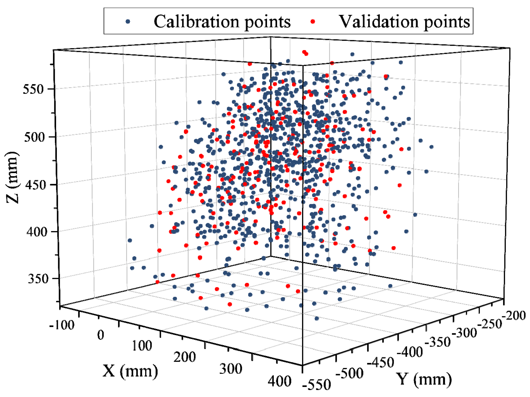
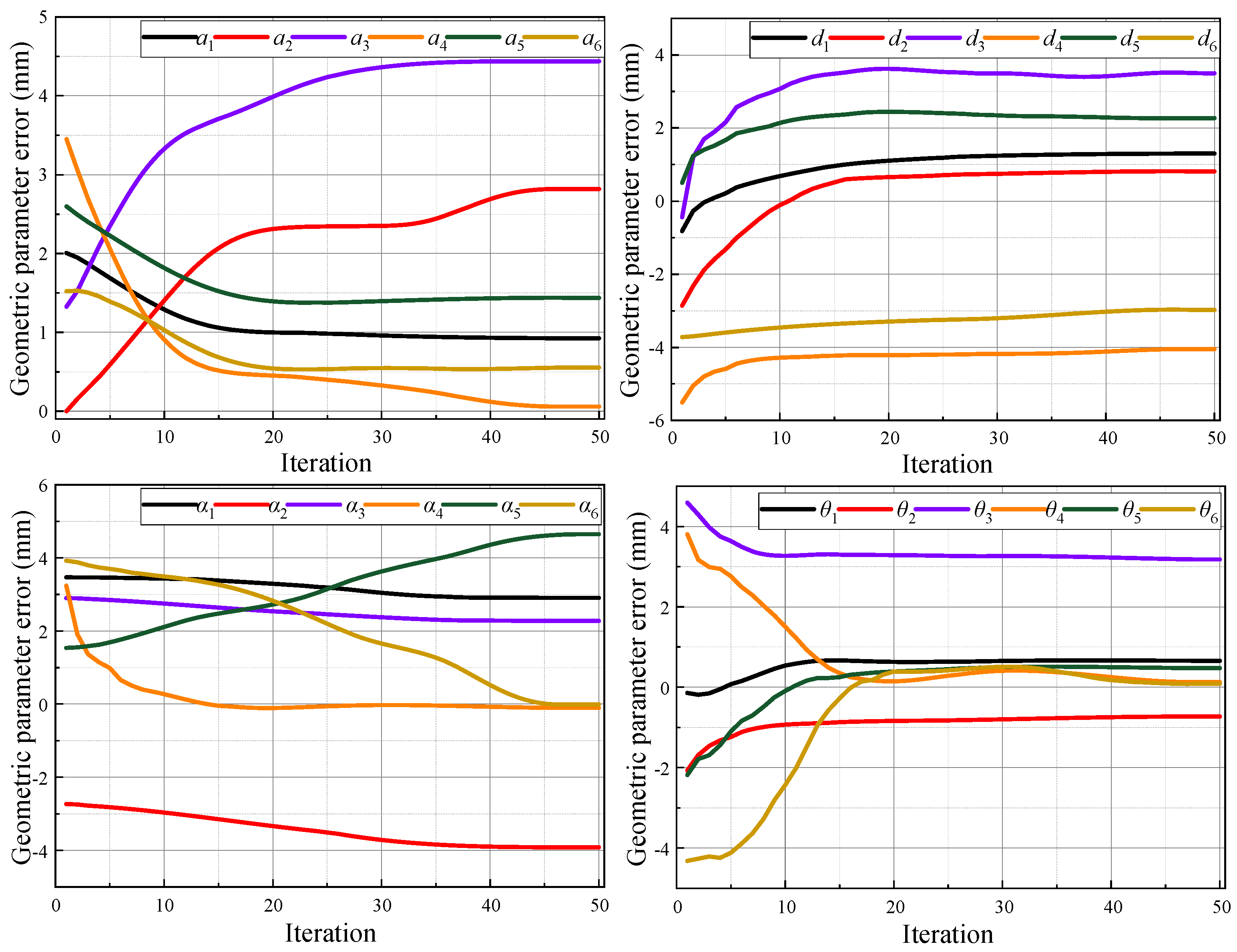
5.2. Experimental Verification of Geometric Parameter Calibration

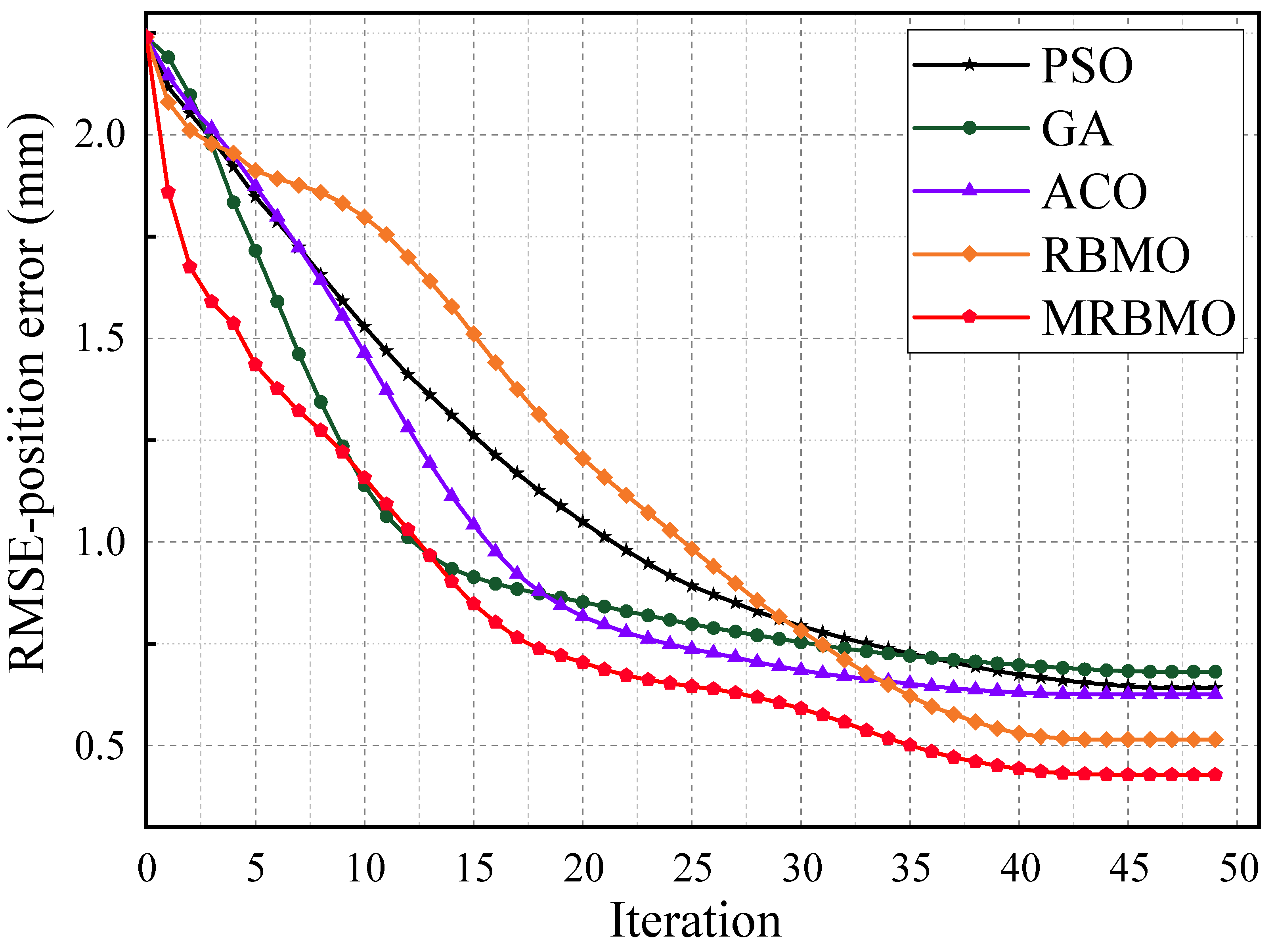
5.2.1. Comparative Method Validation

To verify the effectiveness of the proposed MRBMO-based calibration strategy, a series of comparative experiments are conducted against several representative and state-of-the-art calibration methods. The selected benchmark methods include:

PSO (particle swarm optimization)a widely used swarm intelligence algorithm for parameter optimization in robot calibration [7].

GA (genetic algorithm): an evolutionary approach that explores the parameter space through population-based search and genetic operations [21].

ACO (ant colony optimization): a bio-inspired algorithm that utilizes pheromone-based probabilistic searching to solve combinatorial optimization problems [22].

RBMO (red-billed blue magpie optimizer): a recently proposed nature-inspired optimizer with strong global convergence ability and adaptive search behavior [17].

MRBMO (memory based red-billed blue magpie optimizer): the algorithm proposed in this paper, which incorporates individual memory mechanisms to improve convergence stability and accuracy in geometric calibration.

5.2.2. Result Analysis and Discussion

To comprehensively evaluate the effectiveness of the proposed MRBMO-based robot geometric calibration method, several experiments and statistical analyses were conducted.

Table 3. Identified geometric parameters.

	Nominal Parameter				Identified Parameter
Joint	a (mm)	d (mm)	α (°)	θ (°)	a (mm)	d (mm)	α (°)	θ (°)
1	0	290	−90	0	0.926	291.301	−87.093	0.659
2	270	0	0	−90	272.816	0.815	−3.918	−90.728
3	70	0	−90	0	74.440	3.498	−87.721	3.176
4	0	302	90	0	0.058	297.752	89.898	0.126
5	0	0	−90	0	1.436	2.269	−85.345	0.474
6	0	72	0	0	0.555	69.024	−0.006	0.088

presents the calibrated geometric parameter values identified using the MRBMO algorithm.

Table 4. Evaluation results of different calibration methods.

Metric	Before	PSO	GA	ACO	RBMO	MRBMO
RMSE (mm)	2.240	0.642	0.681	0.625	0.515	0.428
Std(mm)	2.030	0.543	0.594	0.520	0.438	0.391
Max(mm)	3.520	1.410	1.583	1.467	1.312	1.126
Time(s)	/	75.146	92.851	108.215	70.512	82.148

summarizes the calibration results of different algorithms, including RMSE, Std, Max, and the total calibration time, thereby providing a comprehensive overview of both accuracy and efficiency. To assess the statistical significance of the differences in performance,

Table 5. Wilcoxon Signed-Rank test results for RMSE, Std, and Max in Table 2.

Comparison	R+	R−	p-Value *
MRBMO vs. PSO	45	0	0.002
MRBMO vs. GA	45	0	0.002
MRBMO vs. ACO	45	0	0.002
MRBMO vs. RBMO	45	0	0.002

* The accepted hypotheses are based on a threshold significance level of 0.05.

reports the results of the Wilcoxon signed-rank test for the RMSE, Std, and Max metrics listed in Table 4. Furthermore, Figure 5 illustrates the convergence behavior of the 24 identified geometric parameter errors when using the MRBMO algorithm, revealing its optimization trajectory. Figure 6 compares the calibration results of various algorithms, highlighting the superiority of MRBMO in multiple dimensions. Figure 7 depicts the evolution of the RMSE-position error across 50 iterations for each algorithm, showcasing the convergence speed and stability. Finally, Figure 8 presents a visual comparison of robot calibration errors using benchmark optimization methods.

The proposed MRBMO algorithm demonstrates significantly enhanced calibration accuracy compared to conventional methods. As shown in Table 4 and Figure 6a–c, MRBMO achieves the lowest RMSE of 0.428 mm, which is 80.89% lower than before calibration (2.240 mm), 33.33% lower than PSO (0.642 mm), 37.17% lower than GA (0.681 mm), 31.52% lower than ACO (0.625 mm), and 16.70% lower than RBMO (0.515 mm). In terms of Std, MRBMO reduces the value to 0.391 mm, indicating a smoother calibration output; this is 80.73% lower than before calibration (2.030 mm), 28.00% lower than PSO (0.543 mm), 34.18% lower than GA (0.594 mm), 24.81% lower than ACO (0.520 mm), and 10.73% lower than RBMO (0.438 mm). Regarding Max error, MRBMO limits the peak deviation to 1.126 mm, which represents a 68.01% reduction compared to before calibration (3.520 mm), 20.14% lower than PSO (1.410 mm), 28.85% lower than GA (1.583 mm), 23.26% lower than ACO (1.467 mm), and 14.17% lower than RBMO (1.312 mm). These consistent reductions across all metrics verify that MRBMO, as an improvement over RBMO, offers better robustness and precision in geometric parameter calibration. Compared with PSO, GA, and ACO, MRBMO not only achieves lower RMSE, Std, and Max values, but also maintains more stable performance, indicating its superior convergence ability and enhanced calibration accuracy across diverse algorithmic baselines.

Although MRBMO incurs a slightly higher computational cost compared to the original RBMO algorithm, this additional time investment is justified by its substantial gains in calibration accuracy. As shown in Table 4 and Figure 6d, MRBMO requires 82.148 s to complete the calibration process, which is 16.50% longer than RBMO’s 70.512 s. However, it achieves consistently lower RMSE, Std, and Max error across all metrics. Compared to ACO (108.215 s) and GA (92.851 s), MRBMO is not only faster but also significantly more accurate. Although PSO completes the process in 75.146 s, its accuracy is far inferior. Therefore, the slight increase in computation time is a worthwhile trade-off for the improved precision MRBMO delivers. Moreover, the time cost can be further reduced through parallel processing or hardware acceleration techniques, making MRBMO a practical and scalable solution for high-precision robotic calibration applications.

Figure 5. Geometric parameter error identification obtained using the MRBMO algorithm.

Figure 5. Geometric parameter error identification obtained using the MRBMO algorithm.

Figure 6. Comparative calibration results among different algorithms. (a) RMSE; (b) Std; (c) Max; (d) Total time.

Figure 6. Comparative calibration results among different algorithms. (a) RMSE; (b) Std; (c) Max; (d) Total time.

To rigorously assess the effectiveness of the MRBMO algorithm over its counterparts, the Wilcoxon signed-rank test was conducted across multiple performance indicators. As detailed in Table 5, each pairwise comparison between MRBMO and PSO, GA, ACO, and RBMO yielded a positive rank sum (R⁺) of 45, negative rank sum (R⁻) of 0, and a p-value of 0.002. These results are significantly below the 0.05 significance threshold, thus confirming the statistical relevance of the observed performance differences. The test outcomes provide robust evidence that MRBMO consistently outperforms all benchmark algorithms in terms of calibration accuracy and reliability. Importantly, the comparison with RBMO—the baseline version without memory reinforcement—demonstrates that the proposed improvements in the MRBMO framework yield statistically significant gains. These findings validate not only the numerical advantage of MRBMO but also its algorithmic superiority under rigorous non-parametric statistical testing, establishing it as a high-confidence solution for precision calibration tasks.

The convergence performance of different optimization algorithms in terms of RMSE-position error is illustrated in Figure 7. All algorithms exhibit a downward trend in RMSE as the number of iterations increases, indicating effective learning and optimization. However, the convergence speed and final accuracy vary significantly across methods. The proposed MRBMO algorithm consistently outperforms the other approaches throughout the entire iteration process. It demonstrates a faster initial descent and lower steady-state error, ultimately converging to approximately 0.43 mm, which is the smallest among all compared methods. In contrast, the original RBMO converges more slowly and stabilizes around 0.51 mm, highlighting the improvement brought by the memory-based enhancement. Traditional algorithms such as PSO, GA, and ACO exhibit slower convergence rates and higher final errors, stabilizing at 0.64 mm, 0.68 mm, and 0.63 mm, respectively. These results clearly demonstrate that MRBMO not only accelerates the convergence process but also enhances optimization precision. Its superior performance can be attributed to the introduction of memory mechanisms, which effectively guide the population toward promising search regions, reduce premature convergence, and improve solution robustness across iterations.

Figure 7. RMSE-position error evolution over iterations under different algorithms.

Figure 7. RMSE-position error evolution over iterations under different algorithms.

Figure 8. Performance comparison of robot calibration error for benchmark algorithms.

Figure 8. Performance comparison of robot calibration error for benchmark algorithms.

The proposed MRBMO algorithm achieves superior calibration accuracy across all measurement points when compared with other benchmark methods. As shown in Figure 8, the top subplot illustrates the robot’s position error before and after applying the MRBMO calibration. The uncalibrated model exhibits substantial fluctuations in positioning accuracy, with errors often exceeding 2.0 mm and peaking near 3.5 mm. In contrast, MRBMO significantly suppresses these deviations, maintaining most pointwise errors below 1.2 mm, with a relatively smooth distribution and minimal outliers. The bottom subplot provides a detailed comparison of position errors obtained by PSO, GA, ACO, RBMO, and MRBMO across 40 test points. It is evident that MRBMO yields the lowest and most stable error distribution among all tested algorithms. Notably, MRBMO consistently outperforms even RBMO—its baseline variant—highlighting the advantage of the incorporated memory mechanism. Algorithms like GA and ACO show larger error variability, particularly in complex regions, while PSO exhibits slightly more compact errors but inferior consistency. These findings further substantiate the robustness of MRBMO in spatial calibration tasks, demonstrating that it not only improves average positioning accuracy but also ensures more uniform error suppression across the workspace. This uniformity is particularly valuable in high-precision applications, where local errors can compromise system-level performance.

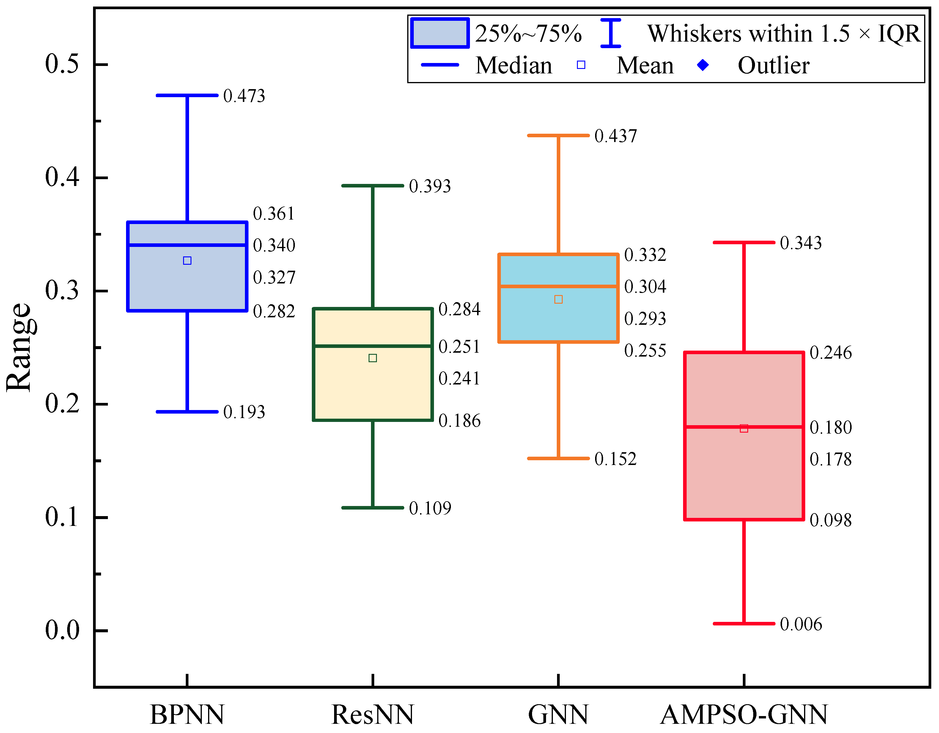
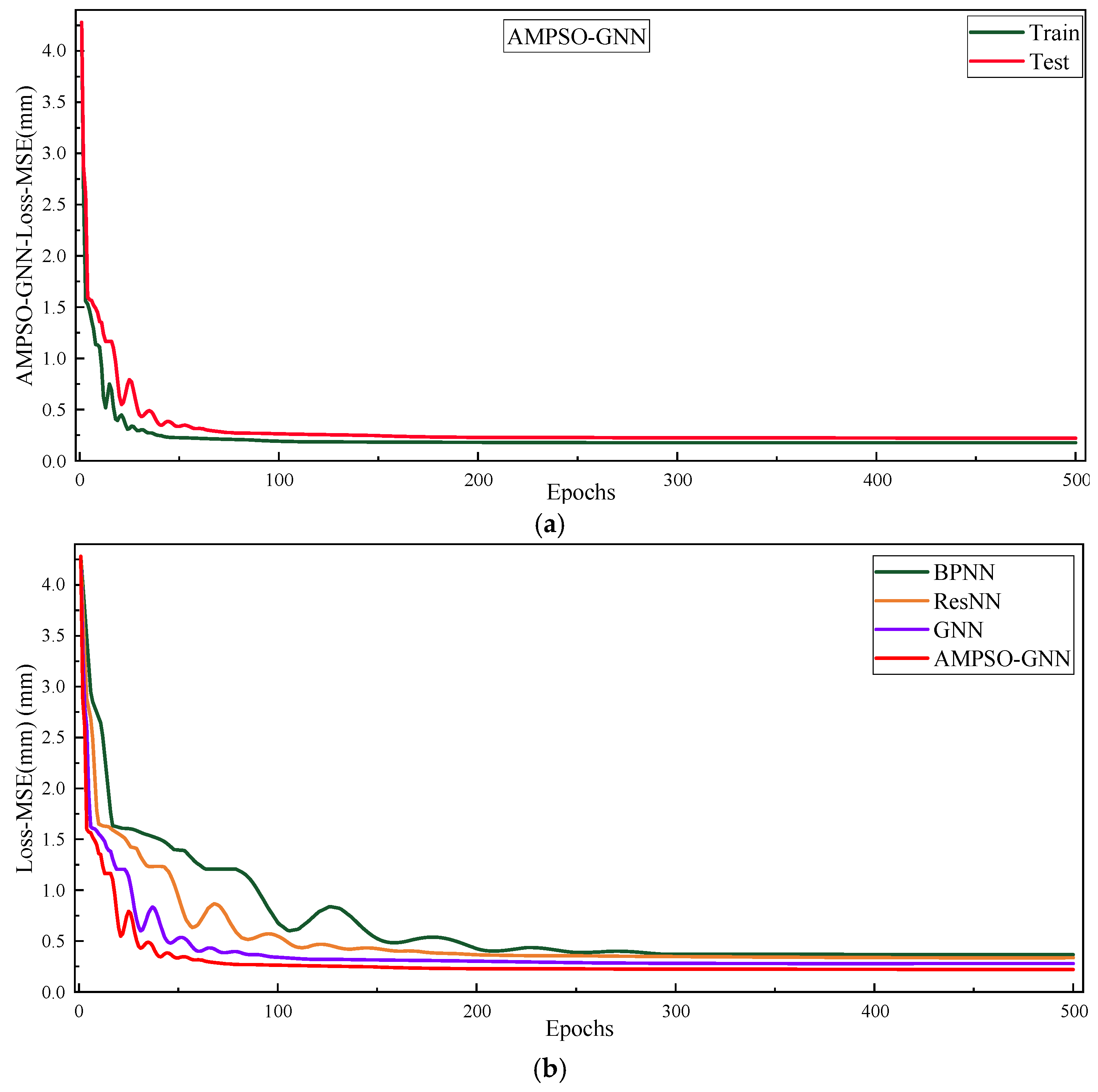
5.3. Experimental Validation of Non-Geometric Calibration

Following the geometric calibration accomplished using the MRBMO algorithm, this section focuses on validating the performance of the proposed AMPSO-GNN model for non-geometric error compensation. To objectively evaluate the effectiveness of AMPSO-GNN, we compare it against three baseline learning models:

BPNN (Backpropagation Neural Network) serves as a classical fully-connected feedforward network, trained using standard gradient descent and widely adopted in early-stage robotic modeling tasks.

ResNN (Residual Neural Network) introduces skip connections to mitigate vanishing gradient issues and enhances training stability, particularly in deeper architectures.

GNN (Graph Neural Network) captures spatial and topological correlations between joint configurations, offering improved generalization over traditional MLP structures.

The architecture of the proposed AMPSO-GNN model comprises three hidden layers, where the number of nodes in each layer is automatically determined by the AMPSO algorithm. The optimization process terminates when either the maximum number of iterations reaches 100 or the fitness value (i.e., prediction error) drops below 0.001 mm. For network training, the number of epochs is fixed at 500, allowing sufficient learning cycles to ensure convergence and stability. In contrast, for baseline comparisons, the BPNN, ResNN, and GNN models are all configured with a fixed architecture of (6, 30, 30, 30, 1), and trained for 500 epochs using standard Levenberg–Marquardt or Adam optimizers.

The evaluation of the AMPSO-GNN model for non-geometric calibration is supported by both quantitative metrics and visual comparisons.

Table 6. Quantitative evaluation of non-geometric calibration models.

		BP	ResNN	GNN	AMPSO-GNN
Network structure		(6, 30, 30, 30, 1)	(6, 30, 30, 30,1)	(6, 30, 30, 30, 1)	3 hidden Layers
Metric	RMSE (mm)	0.354	0.275	0.321	0.220
	Std (mm)	0.315	0.245	0.285	0.196
	Max (mm)	0.625	0.486	0.567	0.389

presents the quantitative evaluation results of different non-geometric calibration models across key performance indicators. Figure 9 compares the performance of several learning-based models in compensating non-geometric errors across measurement points. Figure 10 provides a boxplot analysis of the positioning error range, revealing the distribution characteristics of each model. Additionally, Figure 11 depicts the MSE loss convergence curves during training, including the training/testing performance of AMPSO-GNN and its comparison with other neural network models. Figure 12 illustrates the pointwise positioning accuracy at various calibration stages, including the initial uncalibrated state, geometric calibration using MRBMO, and subsequent non-geometric compensation using AMPSO-GNN.

A detailed comparison of the quantitative evaluation results in Table 6 reveals the superior performance of the proposed AMPSO-GNN model in non-geometric calibration. In terms of RMSE, AMPSO-GNN achieves 0.220 mm, which represents a 37.85% reduction compared to BPNN (0.354 mm), a 20.00% reduction compared to ResNN (0.275 mm), and a 31.46% reduction compared to GNN (0.321 mm). For Std, AMPSO-GNN reaches 0.196 mm, improving upon BPNN (0.315 mm) by 37.78%, ResNN (0.245 mm) by 20.00%, and GNN (0.285 mm) by 31.23%. In terms of the Max, the AMPSO-GNN model achieves a peak error of 0.389 mm, which is 37.76% lower than BPNN (0.625 mm), 19.75% lower than ResNN (0.486 mm), and 31.41% lower than GNN (0.567 mm). These substantial reductions across all metrics demonstrate that the combination of adaptive momentum optimization and graph-based learning significantly enhances the accuracy, consistency, and robustness of non-geometric error compensation.

Figure 9 illustrates the positioning accuracy at each measurement point achieved by different neural network-based models for non-geometric error compensation, including BPNN, ResNN, GNN, and AMPSO-GNN. It can be observed that the accuracy of the traditional BPNN and ResNN models fluctuates considerably across the points, with several instances exhibiting higher local errors exceeding 0.4 mm. While GNN offers slightly better consistency owing to its ability to model spatial dependencies, noticeable variations in error persist. In contrast, the AMPSO-GNN model consistently yields lower positioning errors at most measurement points, and the error distribution is significantly more stable. The use of adaptive momentum-based optimization effectively enhances the representational capacity of the GNN and improves convergence quality, leading to better generalization across the workspace. The denser clustering of red stars at lower vertical positions reflects the robustness and reliability of AMPSO-GNN in compensating for complex non-geometric deviations that traditional models fail to fully capture.

Figure 9. Evaluation of non-geometric error compensation by different neural architectures.

Figure 9. Evaluation of non-geometric error compensation by different neural architectures.

Figure 10 presents a boxplot analysis of the positioning error range across four different non-geometric calibration models: BPNN, ResNN, GNN, and AMPSO-GNN. This statistical visualization captures the central tendency, spread, and outlier distribution of the pointwise positioning errors for each model. As shown, the AMPSO-GNN model exhibits the smallest IQR and the lowest overall spread, with its whiskers extending from 0.006 mm to 0.343 mm, and a median error range of approximately 0.180 mm. In contrast, the BPNN and GNN models show significantly larger IQRs and higher medians (0.327 mm and 0.293 mm, respectively), suggesting greater variability and less stable performance across measurement points. The ResNN model offers slightly improved consistency over BPNN and GNN, but its error range distribution remains broader than that of AMPSO-GNN. Furthermore, the AMPSO-GNN model contains no extreme outliers, while other models display wider whiskers or scattered anomalies. This comparative analysis indicates that AMPSO-GNN not only achieves lower positioning errors but also maintains better stability and robustness, effectively suppressing localized deviations in the calibration process.

Figure 10. Boxplot of positioning error range for different non-geometric calibration models.

Figure 10. Boxplot of positioning error range for different non-geometric calibration models.

Figure 11 illustrates the convergence behavior of the MSE loss during the training process of different learning-based non-geometric calibration models. In Figure 11a, the training and testing loss curves of the AMPSO-GNN model are shown. The model exhibits fast and stable convergence within the first 100 epochs, and both the training and testing curves closely align, indicating strong generalization ability and minimal risk of overfitting. Figure 11b compares the training loss dynamics among BPNN, ResNN, GNN, and AMPSO-GNN. It can be observed that AMPSO-GNN achieves the lowest final loss and the fastest convergence rate. The other models, particularly BPNN and ResNN, converge more slowly and show larger oscillations in the early stages of training. Although GNN performs better than traditional networks, it still falls behind AMPSO-GNN in terms of convergence speed and stability. These results highlight the advantages of integrating adaptive momentum-based optimization into the GNN framework, enabling more effective learning for non-geometric error compensation.

Figure 11. MSE loss convergence curves of learning-based non-geometric calibration models. (a) Training and testing losses of the AMPSO-GNN model; (b) multi-model comparison of training loss dynamics.

Figure 11. MSE loss convergence curves of learning-based non-geometric calibration models. (a) Training and testing losses of the AMPSO-GNN model; (b) multi-model comparison of training loss dynamics.

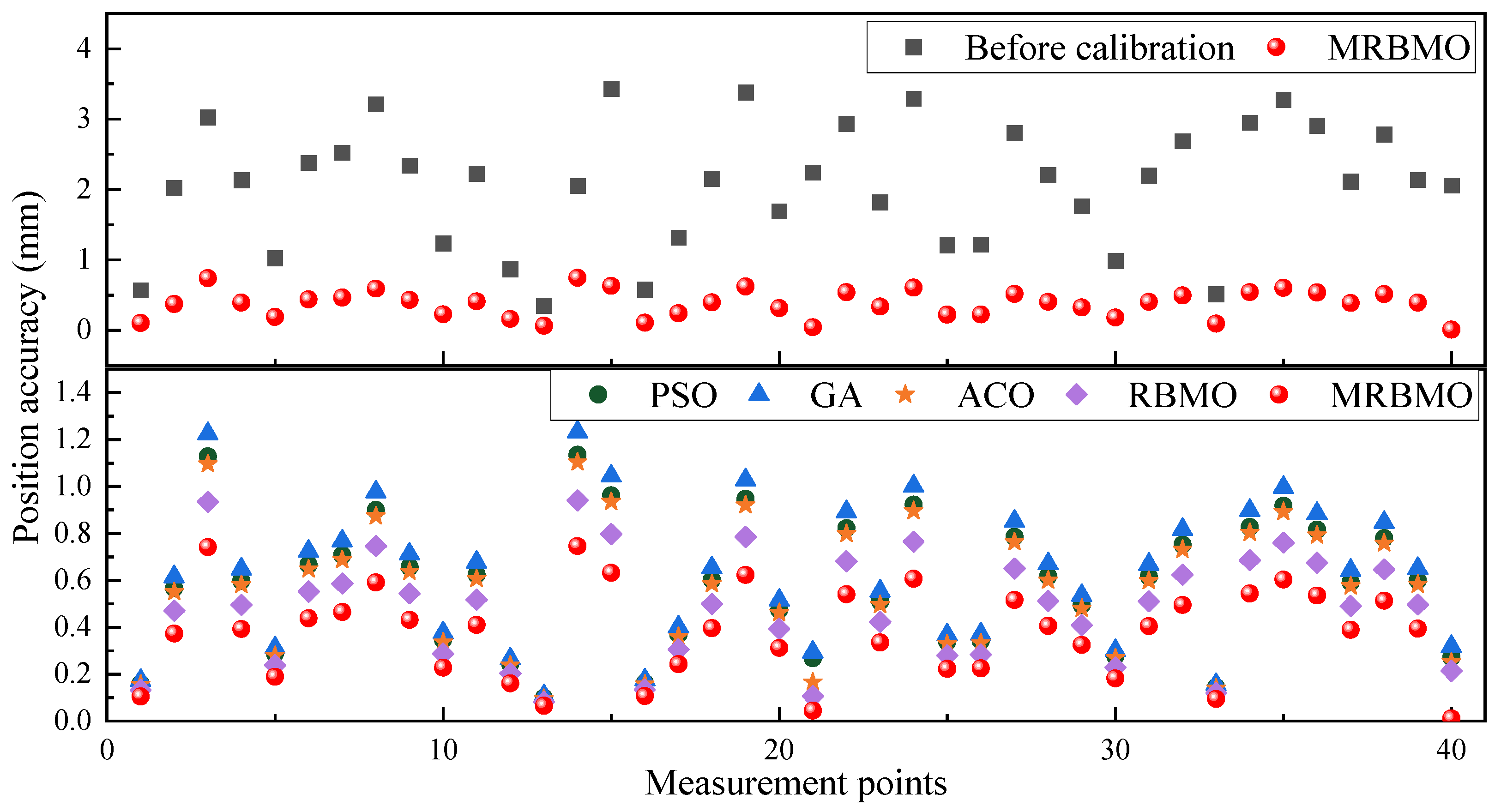
5.4. Overall Positioning Accuracy Improvement Comparison

To comprehensively validate the effectiveness of the proposed dual-stage calibration framework, a three-stage comparative analysis was conducted:

(1)

Before Calibration (uncalibrated),

(2)

After Geometric Calibration using MRBMO, and

(3)

After Full Calibration combining MRBMO and AMPSO-GNN.

The corresponding pointwise error distributions are depicted in Figure 12, while the aggregated statistical results are summarized in

Table 7. Overall comparison of robot positioning accuracy across calibration stages.

Calibration Stage	RMSE (mm)	Std (mm)	Max (mm)
Before Calibration	2.240	2.030	3.520
After Geometric	0.428	0.391	1.126
After Full (MRBMO + AMPSO − GNN)	0.220	0.196	0.389

. As shown, the RMSE decreases significantly from 2.240 mm (uncalibrated) to 0.428 mm after geometric calibration, and further down to 0.220 mm following full compensation. Similarly, the standard deviation and maximum error are notably reduced by 90.34% and 88.94%, respectively. These results confirm that the proposed method substantially enhances positioning accuracy and is well-suited for precision-critical robotic applications.

As further illustrated in Figure 12, the uncalibrated robot exhibits considerable variation and large local positioning errors, with many measurement points exceeding 2.0 mm. After geometric calibration via MRBMO, the overall error level is notably suppressed, though some residual errors remain. Incorporating AMPSO-GNN for non-geometric compensation leads to a consistently lower and more stable pointwise error profile, as evidenced by the concentrated distribution of red triangles. This clearly demonstrates the effectiveness of the GNN-based compensation in correcting residual non-geometric deviations and emphasizes the importance of combining both calibration stages.

Overall, the proposed framework was rigorously validated through both geometric and non-geometric experiments. The MRBMO algorithm effectively identified geometric parameter deviations, while the AMPSO-GNN model successfully compensated for time-varying, nonlinear non-geometric errors. Compared to multiple benchmark algorithms, the proposed approach exhibits superior performance in terms of precision, robustness, and convergence behavior.

Figure 12. Comparison of pointwise positioning accuracy across calibration stages.

Figure 12. Comparison of pointwise positioning accuracy across calibration stages.

6. Conclusions

This paper addresses the challenge of improving the absolute positioning accuracy of industrial robots by proposing a two-stage calibration framework that integrates a memory-enhanced evolutionary optimization method with a neural network-based error compensation strategy. The approach combines a MRBMO for geometric error identification with an AMPSO-GNN for non-geometric error compensation. Based on extensive experimental validation, the following conclusions can be drawn:

(a)

The proposed MRBMO algorithm effectively enhances geometric parameter calibration accuracy by incorporating memory-based guidance into the search process. Compared to conventional optimization methods such as PSO, GA, ACO, and RBMO, MRBMO achieves better convergence and higher identification precision.

(b)

The proposed AMPSO-GNN model significantly outperforms conventional learning-based approaches in compensating non-geometric errors. Compared to BPNN, ResNN, and GNN, AMPSO-GNN achieves lower RMSE, reduced error variability, and faster convergence. These improvements are attributed to the adaptive momentum PSO’s capability to fine-tune GNN hyperparameters, leading to enhanced learning efficiency and generalization ability.

(c)

The combination of MRBMO for geometric calibration and AMPSO-GNN for non-geometric compensation enables a significant improvement in robot positioning accuracy. The two-stage strategy ensures that both systematic kinematic deviations and complex residual errors are effectively addressed, resulting in consistent error suppression across measurement points.

Future work will focus on extending the proposed method to dynamic scenarios involving multi-factor disturbances, such as thermal drift and payload variations. Additionally, integration with real-time control systems and deployment on physical robotic platforms will be explored to further enhance its practical applicability.

References

1. Dehghani, M.; McKenzie, R.A.; Irani, R.A.; Ahmadi, M. Robot-mounted sensing and local calibration for high-accuracy manufacturing. Robot. Comput.-Integr. Manuf. 2023, 79, 102429. [Google Scholar] [CrossRef]
2. Deng, Y.; Hou, X.; Li, B.; Wang, J.; Zhang, Y. A novel method for improving optical component smoothing quality in robotic smoothing systems by compensating path errors. Opt. Express 2023, 31, 30359–30378. [Google Scholar] [CrossRef]
3. Maghami, A.; Imbert, A.; Côté, G.; Monsarrat, B.; Birglen, L.; Khoshdarregi, M. Calibration of multi-robot cooperative systems using deep neural networks. J. Intell. Robot. Syst. 2023, 107, 55. [Google Scholar] [CrossRef]
4. Gao, G.; Zhao, J.; Na, J. Decoupling of kinematic parameter identification for articulated arm coordinate measuring machines. IEEE Access 2018, 6, 50433–50442. [Google Scholar] [CrossRef]
5. Haring, M.; Grøtli, E.I.; Riemer-Sørensen, S.; Seel, K.; Hanssen, K.G. A Levenberg–Marquardt algorithm for sparse identification of dynamical systems. IEEE Trans. Neural Netw. Learn. Syst. 2022, 34, 9323–9336. [Google Scholar] [CrossRef]
6. Deng, Y.; Hou, X.; Li, B.; Wang, J.; Zhang, Y. A highly powerful calibration method for robotic smoothing system calibration via using adaptive residual extended Kalman filter. Robot. Comput.-Integr. Manuf. 2024, 86, 102660. [Google Scholar] [CrossRef]
7. Chen, X.; Zhan, Q. The kinematic calibration of a drilling robot with optimal measurement configurations based on an improved multi-objective PSO algorithm. Int. J. Precis. Eng. Manuf. 2021, 22, 1537–1549. [Google Scholar] [CrossRef]
8. Toquica, J.S.; Motta, J.M.S.T. A novel approach for robot calibration based on measurement sub-regions with comparative validation. Int. J. Adv. Manuf. Technol. 2024, 131, 3995–4008. [Google Scholar] [CrossRef]
9. Cao, H.Q.; Nguyen, H.X.; Tran, T.N.C.; Tran, H.N.; Jeon, J.W. A robot calibration method using a neural network based on a butterfly and flower pollination algorithm. IEEE Trans. Ind. Electron. 2021, 69, 3865–3875. [Google Scholar] [CrossRef]
10. Kong, Y.; Yang, L.; Chen, C.; Zhu, X.; Li, D.; Guan, Q.; Du, G. Online kinematic calibration of robot manipulator based on neural network. Measurement 2024, 238, 115281. [Google Scholar] [CrossRef]
11. Chen, D.; Wang, T.; Yuan, P.; Sun, N.; Tang, H. A positional error compensation method for industrial robots combining error similarity and radial basis function neural network. Meas. Sci. Technol. 2019, 30, 125010. [Google Scholar] [CrossRef]
12. Mon, Y.J. Tikhonov-Tuned Sliding Neural Network Decoupling Control for an Inverted Pendulum. Electronics 2023, 12, 4415. [Google Scholar] [CrossRef]
13. Mon, Y.J. Fuzzy PDC-Based LQR Sliding Neural Network Control for Two-Wheeled Self-Balancing Cart. Electronics 2025, 14, 1842. [Google Scholar] [CrossRef]
14. Pan, J.; Qu, L.; Peng, K. Deep residual neural-network-based robot joint fault diagnosis method. Sci. Rep. 2022, 12, 17158. [Google Scholar] [CrossRef]
15. Guo, J.; Nguyen, H.T.; Liu, C.; Cheah, C.C. Convolutional neural network-based robot control for an eye-in-hand camera. IEEE Trans. Syst. Man Cybern. Syst. 2023, 53, 4764–4775. [Google Scholar] [CrossRef]
16. Zhou, Y.; Xiao, J.; Zhou, Y.; Loianno, G. Multi-robot collaborative perception with graph neural networks. IEEE Robot. Autom. Lett. 2022, 7, 2289–2296. [Google Scholar] [CrossRef]
17. Fu, S.; Li, K.; Huang, H.; Ma, C.; Fan, Q.; Zhu, Y. Red-billed blue magpie optimizer: A novel metaheuristic algorithm for 2D/3D UAV path planning and engineering design problems. Artif. Intell. Rev. 2024, 57, 134. [Google Scholar] [CrossRef]
18. Wu, Z.; Pan, S.; Chen, F.; Long, G.; Zhang, C.; Yu, P.S. A comprehensive survey on graph neural networks. IEEE Trans. Neural Netw. Learn. Syst. 2020, 32, 4–24. [Google Scholar] [CrossRef] [PubMed]
19. Feng, A.; Zhou, Y.; Zhang, R.; Zhao, W.; Li, Z.; Zhu, M. A novel kinematic calibration method for robot based on the Levenberg–Marquardt and improved Marine Predators algorithm. Measurement 2025, 243, 116125. [Google Scholar] [CrossRef]
20. Jiang, X.; Zhang, D.; Wang, H. Positioning error calibration of six-axis robot based on sub-identification space. Int. J. Adv. Manuf. Technol. 2024, 130, 5693–5707. [Google Scholar] [CrossRef]
21. Wang, K. Application of genetic algorithms to robot kinematics calibration. Int. J. Syst. Sci. 2009, 40, 147–153. [Google Scholar] [CrossRef]
22. Wang, X.; Xie, L.; Jiang, M.; He, K.; Chen, Y. Kinematic calibration and feedforward control of a heavy-load manipulator using parameters optimization by an ant colony algorithm. Robotica 2024, 42, 728–756. [Google Scholar] [CrossRef]
Figure 2. Overview of the robotic system and the measurement model based on draw-wire sensor.
Machines 13 00526 g002
Figure 3. Structure of the AMPSO-GNN model.
Machines 13 00526 g003