Direct Force Control Technology for Longitudinal Trajectory of Receiver Aircraft Based on Incremental Nonlinear Dynamic Inversion and Active Disturbance Rejection Controller

Abstract

Aiming at the requirements of rapidity, high precision, and robustness for the longitudinal trajectory control of the receiver aircraft in autonomous aerial refueling, a direct lift control (DLC) strategy that integrates incremental nonlinear dynamic inversion (INDI) and nonlinear extended state observer (NESO) is proposed. First, a control strategy for generating direct lift through the coordinated action of the flaperons and elevators is presented, and a longitudinal dynamics model is established. Secondly, based on the INDI and DLC methods, the rapid tracking and control of altitude are achieved. Finally, an NESO is designed. The observer gains are designed through the pole placement method and the robust optimization method to achieve the estimation of states such as airspeed, angle of attack, pitch rate, and pitch angle, as well as unknown force and moment disturbances. The estimated force and moment disturbances are used to implement the active disturbance rejection control. Simulation results show that the strategy has no altitude tracking error under normal operating conditions, and the altitude tracking error is less than 0.2 m under typical disturbance conditions, indicating high control accuracy. Under disturbance conditions, the estimation errors of true airspeed, angle of attack, pitch angle, and pitch angular velocity are less than 0.3 m/s, 0.12°, 0.1°, and 0.2°/s, respectively, demonstrating the high-precision estimation capability of the observer. The NESO exhibits high accuracy in state estimation, the rudder deflection is smooth, and the anti-disturbance capability is significantly better than traditional methods, providing an engineered solution for the longitudinal control of the receiver aircraft.

1. Introduction

Autonomous aerial refueling (AAR), as a core technology for enhancing the combat-effectiveness of aviation equipment, is a key guarantee for achieving long-range strategic delivery and sustained combat capabilities [1,2,3]. During the AAR process, the longitudinal trajectory control of the receiver aircraft faces multiple challenges. The core research question focuses on how to achieve rapid and high-precision tracking of the receiver aircraft’s longitudinal trajectory under the dual influence of complex external disturbances and nonlinear dynamic characteristics and ensure that the system has strong robustness [4,5,6]. Specifically, first, the conventional control method based on aerodynamic force has a limited response bandwidth, making it difficult to achieve rapid tracking of the rapid changes in the altitude commands of the tanker aircraft [7]. Second, the dynamic model of the receiver aircraft has strong nonlinear characteristics. For example, the aerodynamic coefficients change with the flight state, and conventional linear control methods cannot accurately describe and control these nonlinear characteristics, resulting in a decrease in control performance [8,9]. Third, the receiver aircraft is subject to external disturbances such as atmospheric turbulence and the wake flow of the refueling aircraft. The atmospheric data sensors installed at local positions are unable to accurately measure the flight states. It is difficult to effectively compensate for these disturbances using conventional control methods, which seriously affects the altitude control accuracy of the receiver aircraft [10,11].

In recent years, scholars have carried out a large amount of research on the longitudinal trajectory control of the receiver aircraft during aerial refueling. Some studies have used the classical control method to achieve trajectory tracking by adjusting the parameters of the controller [12], but this method has poor adaptability to the nonlinear characteristics of the system and external disturbances. Other studies have used modern control theories, such as sliding mode control [13], adaptive dynamic surface control [14], L1 adaptive control [15], robust servo control [16], robust cascade observer [17], robust IDA-PBC [18], etc. These methods can improve the robustness and control performance of the system to a certain extent, but for complex nonlinear systems and external disturbances, there are still certain limitations.

With the development of intelligent control technology, some scholars have begun to apply intelligent control methods such as neural networks and fuzzy control to the longitudinal trajectory control of the receiver aircraft [19,20]. These methods have strong adaptability and learning ability and can effectively deal with the nonlinear characteristics of the system and external disturbances. However, the design and implementation of intelligent control methods are relatively complex and require a large amount of training data and computing resources.

Conventional longitudinal control methods such as PID control and LQR control rely on linearized models and are prone to problems of decreased control accuracy and stability under conditions of strong disturbances [21]. Dynamic inversion (DI) control achieves system linearization through nonlinear feedback, but it is sensitive to model errors and has significant high-frequency chattering problems [22]. Although the extended state observer (ESO) can estimate system disturbances, its linear design has estimation delays and insufficient accuracy in strong nonlinear situations [23]. In recent years, the nonlinear extended state observer (NESO) has shown advantages in dealing with complex nonlinear systems. By expanding the state vector, it incorporates unknown disturbances into the observation scope, improving the disturbance suppression ability [24,25]. However, the engineering adaptability of the observer gain design and the control law reported in existing studies studies indicates the need for further in-depth research.

In contrast with other control methods, incremental nonlinear dynamic inversion (INDI) is based on the nonlinear dynamic model of the system. Through dynamic inversion technology, it directly eliminates nonlinear terms; transforms complex nonlinear systems into linear pseudo-dynamic systems; and, thus, achieves precise control across the entire operating range. INDI is typically combined with robust control technologies (such as disturbance observers), introducing compensation terms in the inversion control law. It can estimate system parameter changes and external disturbances (e.g., gusts, load fluctuations) in real time and dynamically adjust control inputs through an incremental form (i.e., based on small changes in the current state), enhancing system robustness. Through dynamic inversion technology, INDI can directly transform the coupled nonlinear system into multiple independent linear subsystems (e.g., decomposing aircraft dynamics into an attitude subsystem and a trajectory subsystem), achieving natural decoupling. This facilitates hierarchical controller design (e.g., outer-loop trajectory planning and inner-loop attitude tracking), reducing design complexity. The “incremental” characteristic of INDI is reflected in that the control law is based on the incremental change of the system state (rather than the absolute state), making it more suitable for handling minor adjustments in dynamic processes. Incremental control enables smoother transitions and higher steady-state accuracy.

Aiming at the above problems, this paper proposes a method for controlling the longitudinal trajectory of the receiver aircraft based on direct lift and an NESO. The innovations of this method are mainly reflected in the following three aspects:

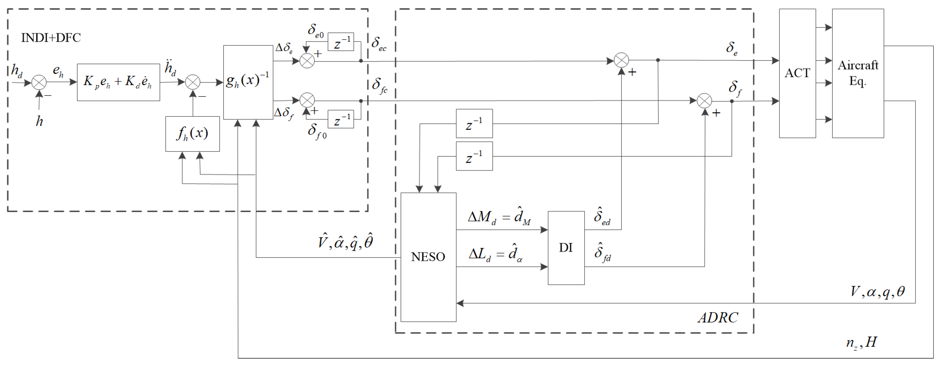
• Novel control strategy integration: We propose a hybrid control framework combining INDI-based direct lift control (DLC) with an NESO, addressing the longitudinal trajectory control challenge for receiver aircraft in aerial refueling. This integration enables fast altitude tracking while suppressing wind disturbances, a gap in existing single-model control approaches.
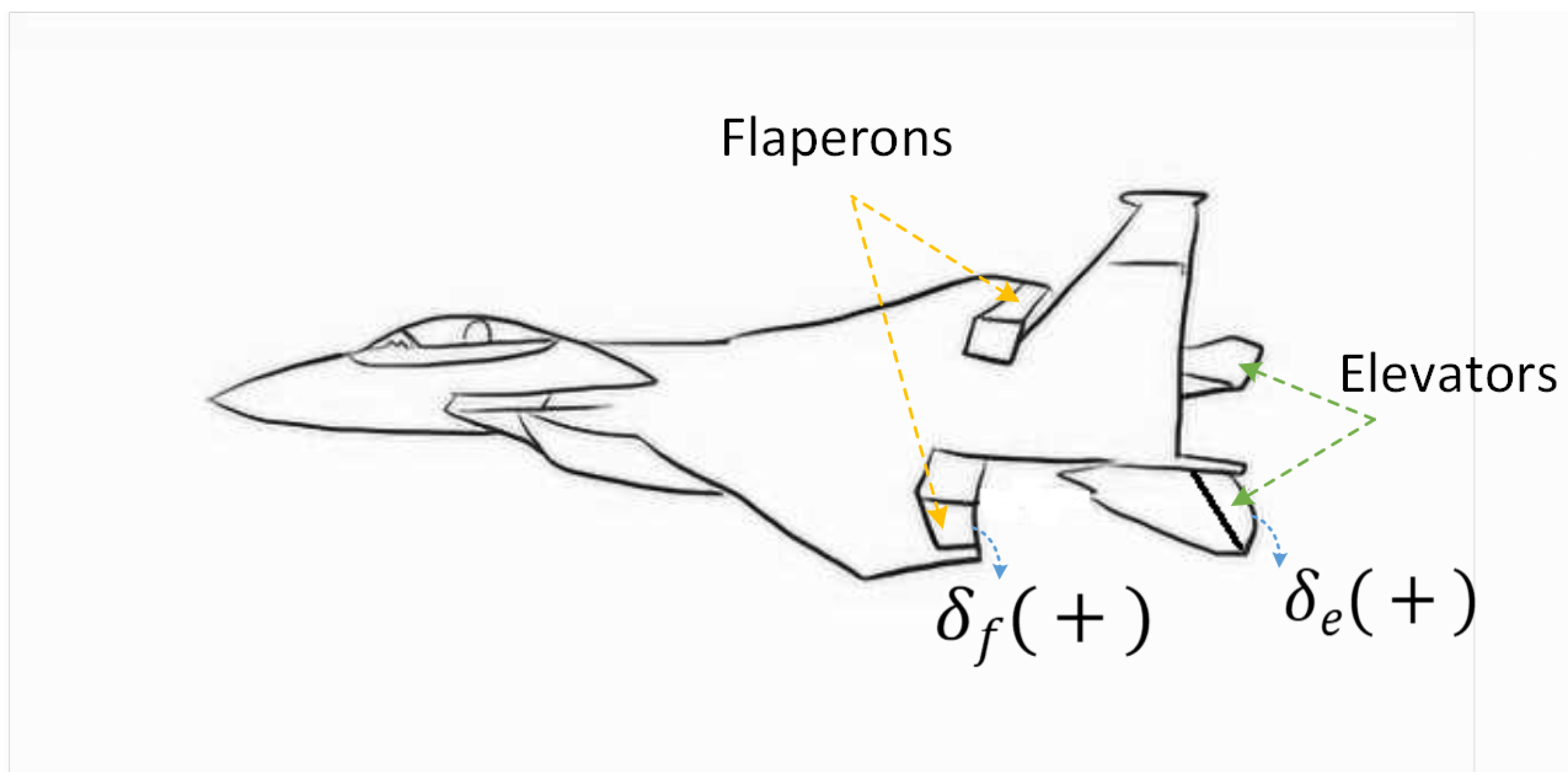
• Collaborative control mechanism: We develop a DLC strategy via symmetric flaperon–elevator coordination, bypassing conventional aerodynamic delays. This mechanism establishes a new longitudinal dynamics model that achieves sub-0.2 m altitude tracking accuracy under moderate Dryden wind conditions.
• Disturbance estimation and compensation: We design an NESO with optimized gains via pole configuration and robust enhancement, enabling real-time estimation of and compensation for external wind disturbances and internal model uncertainties. This addresses the limitation of conventional observers in dynamic environments, as proven by Lyapunov stability analysis.

These contributions collectively advance the state-of-the-art in receiver aircraft control, particularly in integrating rapid response, disturbance rejection, and real-time performance for critical mid-air refueling scenarios. The research results of this paper provide a theoretical and engineering solution for the longitudinal control of the receiver aircraft in AAR and are of significance for the promotion of the development of AAR technology.

The rest of this paper is organized as follows. A DLC strategy and longitudinal dynamics modeling of the receiver aircraft are introduced in Section 2. The architecture of the altitude control law is presented in Section 3. The NESO for the receiver aircraft is designed in Section 4. The longitudinal altitude tracking control law is presented in Section 5. The simulation test and analysis are of the results are provided in Section 6. Finally, the conclusions are summarized in Section 7.

It should be explained that in the context of aerial refueling (air-to-air refueling), receiver and tanker refer to specific aircraft roles with distinct functions. Below is a detailed definition of each term: A receiver, which is also known as a “recipient” or “client aircraft”, is defined as an aircraft that receives fuel from another aircraft (the tanker) during aerial refueling. A tanker, which is also called a “refueling aircraft” or “airborne fuel tanker”, is defined as an aircraft specifically designed or modified to transfer fuel to other aircraft (receiver) during flight.

2. DLC Strategy and Longitudinal Dynamics Modeling of the Receiver Aircraft

2.1. Direct Lift Generation Mechanism

DLC can directly provide additional lift through the coordination of control surfaces without changing the flight attitude of the aircraft, enabling the aircraft to make a translational movement in the vertical direction to change its flight path. The direct lift discussed in this paper is generated by the co-directional deflection of the flaperons (${\delta }_f$), and the coordinated deflection of the elevator (${\delta }_e$) is used to counteract the pitching moment generated by the normal deflection of the flaperons.

Flaperons are used as follows: By deflecting synchronously, they alter the lift on the wing’s symmetry plane. The deflection angle ranges from ${\delta }_{fmin}$ to ${\delta }_{fmax}$, with corresponding lift coefficient derivative $C_{L{\delta }_f}$ and drag coefficient derivative $C_{D{\delta }_f}$.

Elevators are used as follows: Their deflection alters the aerodynamic load at the aircraft’s tail, adjusting the angle of attack and pitching attitude. The deflection angle ranges from ${\delta }_{emin}$ to ${\delta }_{emax}$, with corresponding lift coefficient derivative $C_{L{\delta }_e}$ and drag coefficient derivative $C_{D{\delta }_e}$. A schematic diagram of the aircraft configuration and direct-force rudder surface configuration is shown in Figure 1.

2.2. Longitudinal Force Equations

In the trajectory coordinate system, the longitudinal dynamics of the receiver aircraft are described by the tangential and normal force balance equations. The state vector is defined as $x={[V,\alpha ,q,\theta ]}^T$, where V is the true airspeed, $\alpha$ is the angle of attack, q is the pitch rate, and $\theta$ is the pitch angle.

The tangential dynamics equation is presented as follows.

$$m\dot{V}=Tcos\alpha -D-mgsin\gamma$$

(1)

The expression for the drag (D) is

$$D={\displaystyle \frac{1}{2}}\rho V^{2}S\left[C_{D0}+C_{D\alpha }\alpha +C_{D{\delta }_f}{\delta }_f+C_{D{\delta }_e}{\delta }_e\right]$$

(2)

where $C_{D0}$ is the zero drag coefficient, $C_{D\alpha }$ is the drag coefficient derivative with respect to the angle of attack, $\rho$ is the air density, S is the wing area, g is the gravitational acceleration, and $\gamma =\theta -\alpha$ is the flight-path angle.

The normal dynamics equation is presented as follows:

$$mV\dot{\gamma }=Tsin\alpha +L-mgcos\gamma$$

(3)

The expression for the lift (L) is

$$L={\displaystyle \frac{1}{2}}\rho V^{2}S\left[C_{L0}+C_{L\alpha }\alpha +C_{L{\delta }_f}{\delta }_f+C_{L{\delta }_e}{\delta }_e\right]$$

(4)

where $C_{L0}$ is the zero lift coefficient and $C_{L\alpha }$ is the lift coefficient derivative with respect to the angle of attack.

2.3. Pitching Moment Equation

Considering the hinge moment coefficients of the control surfaces ($C_{M{\delta }_f}$ for flaperons and $C_{M{\delta }_e}$ for the elevator), the expression for the pitching moment (M) is

$$M={\displaystyle \frac{1}{2}}\rho V^{2}S\overline{c}\left[C_{M0}+C_{M\alpha }\alpha +C_{Mq}q+C_{M{\delta }_f}{\delta }_f+C_{M{\delta }_e}{\delta }_e\right]$$

(5)

where $\overline{c}$ is the mean aerodynamic chord length, $C_{M0}$ is the zero pitching moment coefficient, $C_{M\alpha }$ is the pitching moment coefficient derivative with respect to the angle of attack, and $C_{Mq}$ is the derivative of the pitch rate. According to the law of rotation, the following equation can be obtained.

$$I_y\dot{q}=M$$

(6)

where $I_y$ is the moment of inertia about the transverse axis.

3. The Altitude Control Law Architecture for the Receiver Aircraft

The longitudinal trajectory control of the receiver aircraft introduced in this paper refers to the altitude tracking and control of the receiver aircraft. The altitude control law of the receiver aircraft is the longitudinal control mode during autonomous aerial refueling docking, which is used to achieve the longitudinal tracking and control of the refueling drogue. On the one hand, this control law uses the INDI and DLC methods to generate the longitudinal control commands of the aircraft: the symmetric flaperon control command (${\widehat{\delta }}_{fc}$) and the elevator control command (${\widehat{\delta }}_{ec}$). On the other hand, it uses an NESO to observe the disturbed state of the aircraft, as well as the disturbing forces and moments. The observed direct forces and moments are used as direct force compensation control to suppress disturbances, and the observed states are used as feedback signals for the INDI control. The altitude control law architecture of the receiver aircraft is mainly divided into two parts: the altitude control module based on INDI and DLC and the ADRC module based on the NESO (which is divided into the NESO module and the disturbance compensation module), as shown in Figure 2. The control objective of the receiver aircraft is to quickly track the given altitude command, such as the predicted drogue altitude.

The input and output of each module are described as follows.

1. Altitude control module based on INDI and DLC

Inputs: altitude command ($h_d$), observer output state ($\widehat{x}$), and measured output state (x).

Outputs: elevator control command (${\delta }_{ec}$), flaperon control command (${\delta }_{ac}$), and rudder control command (${\delta }_{rc}$).

2. NESO module:

Inputs: control surface deflection angles (${\delta }_f,{\delta }_e$) and measured values ($V,\alpha ,q,\theta$).

Outputs: state estimate ($\widehat{x}$) and disturbance estimate ($\widehat{d}$).

3. Disturbance compensation module:

Inputs: lift disturbance ($\Delta L_d$) and pitching moment disturbance ($\Delta M_d$).

Outputs: control surface deflection angles (${\widehat{\delta }}_{fc},{\widehat{\delta }}_{ec}$), which are solved by the pseudo-inverse method:

$$\left[\begin{array}{c}{\widehat{\delta }}_{fd}\\ {\widehat{\delta }}_{ed}\end{array}\right]={\left(G_L^T{G}_L\right)}^{-1}{G}_L^T\left[\begin{array}{c}\Delta L_d\\ \Delta M_d\end{array}\right]$$

(7)

where $\widehat{x}=\left[\widehat{V},\widehat{\alpha },\widehat{q},\widehat{\theta }\right]$, $x=\left[n_z,H\right]$, and $G_L=\left[\begin{array}{cc}{C}_{L{\delta }_a}& C_{L{\delta }_e}\\ C_{M{\delta }_a}& C_{M{\delta }_e}\end{array}\right]$ is the influence matrix of the control surface. Here, $n_z$ represents the normal load factor.

4. The NESO for the Receiver Aircraft

4.1. General Design Method of the NESO

Consider a nonlinear system

$$\left\{\begin{array}{c}\dot{\mathit{x}}=\mathit{f}(\mathit{x},\mathit{u},\mathit{d})\hfill \\ \mathit{y}=\mathit{h}\left(\mathit{x}\right)\hfill \end{array}\right.$$

where $\mathit{x}\in {\mathbb{R}}^n$ is the state vector (including dynamic parameters such as true airspeed and angle of attack), $\mathit{u}\in {\mathbb{R}}^m$ is the control input (such as control surface deflection angles), $\mathit{d}\in {\mathbb{R}}^p$ is the external disturbance vector (including aerodynamic disturbances and wind-field perturbations), and $\mathit{y}\in {\mathbb{R}}^q$ is the measured output.

The NESO transforms the disturbance term into an estimable state by augmenting the state vector ($\mathit{z}={[{\mathit{x}}^T,{\mathit{d}}^T]}^T$) and constructs an observation system:

$$\dot{\widehat{\mathit{z}}}=\left[\begin{array}{c}\mathit{f}(\widehat{\mathit{x}},\mathit{u},\widehat{\mathit{d}})\\ \mathbf{0}\end{array}\right]+\mathit{L}(\mathit{y}-\mathit{h}\left(\widehat{\mathit{x}}\right))$$

(8)

where $\widehat{\mathit{x}}$ and $\widehat{\mathit{d}}$ are the estimated values of the state and the disturbance, respectively; $\mathit{L}={[{\mathit{L}}_x^T,{\mathit{L}}_d^T]}^T$ is the block gain matrix, where ${\mathit{L}}_x\in {\mathbb{R}}^{n\times q}$ is used to adjust the convergence rate of the state estimation and ${\mathit{L}}_d\in {\mathbb{R}}^{p\times q}$ is used for disturbance estimation compensation. The observer uses the output error ($\mathit{y}-\mathit{h}\left(\widehat{\mathit{x}}\right)$) to drive the iteration of the estimated values and realizes fast and accurate state and disturbance estimation by optimizing $\mathit{L}$.

4.2. Design of the State Observer for the Receiver Aircraft

4.2.1. State Equation Modeling

The longitudinal dynamics state vector is set as $\mathit{x}={[V,\alpha ,q,\theta ]}^T$ (true airspeed, angle of attack, pitch rate, and pitch angle), the control input is set as $\mathit{u}={[{\delta }_f,{\delta }_e]}^T$ (symmetric deflection angle of the flaperons and elevator deflection angle), and the output is set as $\mathit{y}=\mathit{x}$. Combining with the dynamic equations is Section 2, the state derivative can be expressed as follows:

$$\dot{\mathit{x}}=\left[\begin{array}{c}{\displaystyle \frac{Tcos\alpha -\frac{1}{2}\rho V^{2}S{C}_D-mgsin(\theta -\alpha )+d_V}{m}}\\ \\ {\displaystyle \frac{Tsin\alpha +\frac{1}{2}\rho V^{2}S{C}_L-mgcos(\theta -\alpha )}{mV}}+{\displaystyle \frac{d_{\alpha }}{mV}}\\ \\ {\displaystyle \frac{\frac{1}{2}\rho V^{2}S\overline{c}{C}_M+d_M}{I_y}}\\ \\ q\end{array}\right]$$

(9)

where $C_L=C_{L0}+C_{L\alpha }\alpha +C_{L{\delta }_f}{\delta }_f+C_{L{\delta }_e}{\delta }_e$, $C_D=C_{D0}+C_{D\alpha }\alpha +C_{D{\delta }_f}{\delta }_f+C_{D{\delta }_e}{\delta }_e$, $C_M=C_{M0}+C_{M\alpha }\alpha +C_{Mq}q+C_{M{\delta }_f}{\delta }_f+C_{M{\delta }_e}{\delta }_e$.

4.2.2. Construction of the Observer Equation

The observer for the receiver aircraft is designed based on the following general method:

$$\left\{\begin{array}{c}\dot{\widehat{\mathit{x}}}=\left[\begin{array}{c}{\displaystyle \frac{Tcos\widehat{\alpha }-\frac{1}{2}\rho {\widehat{V}}^{2}S{C}_D(\widehat{\mathit{x}},\mathit{u})-mgsin(\widehat{\theta }-\widehat{\alpha })+{\widehat{d}}_V}{m}}\\ \\ {\displaystyle \frac{Tsin\widehat{\alpha }+\frac{1}{2}\rho {\widehat{V}}^{2}S{C}_L(\widehat{\mathit{x}},\mathit{u})-mgcos(\widehat{\theta }-\widehat{\alpha })}{m\widehat{V}}}+{\displaystyle \frac{{\widehat{d}}_{\alpha }}{m\widehat{V}}}\\ \\ {\displaystyle \frac{\frac{1}{2}\rho {\widehat{V}}^{2}S\overline{c}{C}_M(\widehat{\mathit{x}},\mathit{u})+{\widehat{d}}_M}{I_y}}\\ \\ \widehat{q}\end{array}\right]+{\mathit{L}}_x(\mathit{y}-\widehat{\mathit{x}})\hfill \\ \dot{\widehat{\mathit{d}}}={\mathit{L}}_d(\mathit{y}-\widehat{\mathit{x}})\hfill \end{array}\right.$$

(10)

where the observer incorporates the thrust disturbance of the true airspeed ($d_V$), the lift disturbance ($d_{\alpha }$), and the pitching moment disturbance ($d_M$) into the estimation scope. By synchronously updating the estimated values of the state and the disturbance, it realizes a comprehensive observation of the longitudinal dynamics of the receiver aircraft.

4.3. Design of the Observer Gain

4.3.1. Linearization of the Error System

When designing the NESO, in order to design the observer gain and analyze its performance, it is necessary to linearize the equation of system error. This process is based on Taylor expansion and is approximated near the equilibrium point $({\mathit{x}}^{*},{\mathit{u}}^{*})$, transforming the complex nonlinear system into a linear form that is convenient for analysis.

The observer equations are

$$\left\{\begin{array}{c}\dot{\widehat{\mathit{x}}}=\mathit{f}(\widehat{\mathit{x}},\mathit{u},\widehat{\mathit{d}})+{\mathit{L}}_x(\mathit{y}-\widehat{\mathit{x}})\hfill \\ \dot{\widehat{\mathit{d}}}={\mathit{L}}_d(\mathit{y}-\widehat{\mathit{x}})\hfill \end{array}\right.$$

(11)

The estimation errors are defined as ${\mathit{e}}_x=\mathit{x}-\widehat{\mathit{x}}$ and ${\mathit{e}}_d=\mathit{d}-\widehat{\mathit{d}}$. Then, ${\dot{\mathit{e}}}_x$ is derived as

$${\dot{\mathit{e}}}_x=\dot{\mathit{x}}-\dot{\widehat{\mathit{x}}}=\mathit{f}(\mathit{x},\mathit{u},\mathit{d})-\mathit{f}(\widehat{\mathit{x}},\mathit{u},\widehat{\mathit{d}})-{\mathit{L}}_x(\mathit{y}-\widehat{\mathit{x}})$$

(12)

Since $\mathit{y}=\mathit{x}$, then

$${\dot{\mathit{e}}}_x=\mathit{f}(\mathit{x},\mathit{u},\mathit{d})-\mathit{f}(\widehat{\mathit{x}},\mathit{u},\widehat{\mathit{d}})-{\mathit{L}}_x(\mathit{x}-\widehat{\mathit{x}})$$

(13)

$\mathit{f}(\mathit{x},\mathit{u},\mathit{d})$ is expanded in a Taylor series at the equilibrium point $({\mathit{x}}^{*},{\mathit{u}}^{*})$ as follows.

$$\left\{\begin{array}{c}\mathit{f}(\mathit{x},\mathit{u},\mathit{d})\approx \mathit{f}({\mathit{x}}^{*},{\mathit{u}}^{*},{\mathit{d}}^{*})+{\displaystyle \frac{\partial \mathit{f}}{\partial \mathit{x}}}{|}_{{\mathit{x}}^{*},{\mathit{u}}^{*}}(\mathit{x}-{\mathit{x}}^{*})+{\displaystyle \frac{\partial \mathit{f}}{\partial \mathit{d}}}{|}_{{\mathit{x}}^{*},{\mathit{u}}^{*}}(\mathit{d}-{\mathit{d}}^{*})\hfill \\ \mathit{f}(\widehat{\mathit{x}},\mathit{u},\widehat{\mathit{d}})\approx \mathit{f}({\mathit{x}}^{*},{\mathit{u}}^{*},{\mathit{d}}^{*})+{\displaystyle \frac{\partial \mathit{f}}{\partial \mathit{x}}}{|}_{{\mathit{x}}^{*},{\mathit{u}}^{*}}(\widehat{\mathit{x}}-{\mathit{x}}^{*})+{\displaystyle \frac{\partial \mathit{f}}{\partial \mathit{d}}}{|}_{{\mathit{x}}^{*},{\mathit{u}}^{*}}(\widehat{\mathit{d}}-{\mathit{d}}^{*})\hfill \end{array}\right.$$

(14)

The above equation is substituted into the expression of ${\dot{\mathit{e}}}_x$. The following formula is obtained.

$${\dot{\mathit{e}}}_x\approx {\displaystyle \frac{\partial \mathit{f}}{\partial \mathit{x}}}{|}_{{\mathit{x}}^{*},{\mathit{u}}^{*}}(\mathit{x}-\widehat{\mathit{x}})+{\displaystyle \frac{\partial \mathit{f}}{\partial \mathit{d}}}{|}_{{\mathit{x}}^{*},{\mathit{u}}^{*}}(\mathit{d}-\widehat{\mathit{d}})-{\mathit{L}}_x(\mathit{x}-\widehat{\mathit{x}})=\left({\displaystyle \frac{\partial \mathit{f}}{\partial \mathit{x}}}{|}_{{\mathit{x}}^{*},{\mathit{u}}^{*}}-{\mathit{L}}_x\right){\mathit{e}}_x+{\displaystyle \frac{\partial \mathit{f}}{\partial \mathit{d}}}{|}_{{\mathit{x}}^{*},{\mathit{u}}^{*}}{\mathit{e}}_d$$

(15)

Let $\mathit{A}={\displaystyle \frac{\partial \mathit{f}}{\partial \mathit{x}}}{|}_{{\mathit{x}}^{*},{\mathit{u}}^{*}}$ and $\mathit{B}={\displaystyle \frac{\partial \mathit{f}}{\partial \mathit{d}}}{|}_{{\mathit{x}}^{*},{\mathit{u}}^{*}}$, then,

$${\dot{\mathit{e}}}_x=\mathit{A}{\mathit{e}}_x+\mathit{B}{\mathit{e}}_d-{\mathit{L}}_x{\mathit{e}}_x=(\mathit{A}-{\mathit{L}}_x){\mathit{e}}_x+\mathit{B}{\mathit{e}}_d$$

(16)

where $\mathit{A}$ is the Jacobian matrix of the system with respect to the state ($\mathit{x}$), describing the influence of the nominal dynamics on the state error, and $\mathit{B}$ is the Jacobian matrix of the system with respect to the disturbance ($\mathit{d}$), representing the coupling effect of the disturbance on the state error. Then, ${\dot{\mathit{e}}}_d$ is given as

$${\dot{\mathit{e}}}_d=\dot{\mathit{d}}-\dot{\widehat{\mathit{d}}}$$

(17)

Assume that the derivative ($\dot{\mathit{d}}$) of the disturbance ($\mathit{d}$) is 0, then,

$${\dot{\mathit{e}}}_d=-{\mathit{L}}_d(\mathit{y}-\widehat{\mathit{x}})=-{\mathit{L}}_d{\mathit{e}}_x$$

(18)

In summary, combining ${\dot{\mathit{e}}}_x$ and ${\dot{\mathit{e}}}_d$ yields the following linearized equation of system error

$$\left[\begin{array}{c}{\dot{\mathit{e}}}_x\\ {\dot{\mathit{e}}}_d\end{array}\right]=\left[\begin{array}{cc}\mathit{A}-{\mathit{L}}_x& \mathit{B}\\ -{\mathit{L}}_d& \mathbf{0}\end{array}\right]\left[\begin{array}{c}{\mathit{e}}_x\\ {\mathit{e}}_d\end{array}\right]$$

(19)

In this way, the linearized equation of the observer system error at the equilibrium point $({\mathit{x}}^{*},{\mathit{u}}^{*})$ is obtained.

4.3.2. Pole Placement Strategy

Pole placement is achieved through the following two steps.

Step 1: Performance index mapping

The desired convergence rate and damping characteristics are set according to the dynamic response requirements of the system. The natural frequency (${\omega }_n$) determines the error convergence rate. The larger ${\omega }_n$ is, the faster the response is; the damping ratio ($\zeta$) adjusts the overshoot. Usually, $0<\zeta <1$ is taken to achieve under-damped and fast convergence.

The desired poles (${\lambda }_i$; $i=1,\cdots ,n+p$) are calculated as

$${\lambda }_i=\left\{\begin{array}{cc}-\zeta {\omega }_n\pm j{\omega }_n\sqrt{1-{\zeta }^2},\hfill & \text{Complex}\text{poles}(\text{oscillatory}\text{parts})\hfill \\ -{\omega }_n,\hfill & \text{Real}\text{poles}(\text{non-oscillatory}\text{parts})\hfill \end{array}\right.$$

(20)

Step 2: Solution of the gain matrix

${\mathit{L}}_x$ and ${\mathit{L}}_d$ are solved by matching the characteristic polynomial of the error system with the desired polynomial:

$$\left\{\begin{array}{c}det(s\mathit{I}-(\mathit{A}-{\mathit{L}}_x))={\prod }_{i=1}^n(s-{\lambda }_i)\hfill \\ det(s\mathit{I}+{\mathit{L}}_d)={\prod }_{i=n+1}^{n+p}(s-{\lambda }_i)\hfill \end{array}\right.$$

(21)

The Ackermann formula or a numerical solution based on the pseudo-inverse is used to transform the pole placement problem into the solution of a system of linear equations.

4.3.3. Robustness Enhancement Optimization Design

In the design of the observer gain, pole placement can enable the observer to achieve the desired dynamic performance. However, in order to further suppress the influence of measurement noise and model mismatch, it is necessary to introduce Lyapunov constraints on the basis of pole placement for robustness enhancement optimization.

First, the constrains of the Lyapunov function are constructed.

The quadratic form of the Lyapunov function id defined as follows:

$$V={\mathit{e}}_x^T\mathit{P}{\mathit{e}}_x+{\mathit{e}}_d^T\mathit{Q}{\mathit{e}}_d$$

(22)

where $\mathit{P}\in {\mathbb{R}}^{n\times n}$ and $\mathit{Q}\in {\mathbb{R}}^{p\times p}$ are positive definite matrices. The selection of these two positive definite matrices is crucial. They are usually determined by solving the Lyapunov equation. The general form of the Lyapunov equation is presented as follows: for a given matrix $\mathit{A}$, if there exists a positive definite matrix ($\mathit{P}$) such that ${\mathit{A}}^T\mathit{P}+\mathit{P}\mathit{A}=-\mathit{Q}$ (where $\mathit{Q}$ is another given positive definite matrix), then $\mathit{P}$ can be solved. In the context of this study, the selection of $\mathit{P}$ and $\mathit{Q}$ needs to comprehensively consider the characteristics and performance requirements of the system. For example, in the dynamic system of the receiver aircraft, different flight states and disturbance characteristics affect the selection of the positive definite matrices. For a flight stage with fast response and high stability requirements, it may be necessary to select $\mathit{P}$ and $\mathit{Q}$ matrices that make the rate of change of the Lyapunov function more negative so as to accelerate the error convergence rate and enhance the system’s stability.

Second, the constraints of the linear matrix inequality (LMI) are defined. Differentiating V yields

$$\dot{V}={({\mathit{e}}_x^T\mathit{P}{\mathit{e}}_x+{\mathit{e}}_d^T\mathit{Q}{\mathit{e}}_d)}^{\prime }={\dot{\mathit{e}}}_x^T\mathit{P}{\mathit{e}}_x+{\mathit{e}}_x^T\mathit{P}{\dot{\mathit{e}}}_x+{\dot{\mathit{e}}}_d^T\mathit{Q}{\mathit{e}}_d+{\mathit{e}}_d^T\mathit{Q}{\dot{\mathit{e}}}_d$$

(23)

The system error (Equation (19)) is substituted into the above formula as follows:

$$\left\{\begin{array}{c}{\dot{\mathit{e}}}_x=\mathit{A}{\mathit{e}}_x+\mathit{B}{\mathit{e}}_d-{\mathit{L}}_x{\mathit{e}}_x=(\mathit{A}-{\mathit{L}}_x){\mathit{e}}_x+\mathit{B}{\mathit{e}}_d\hfill \\ {\dot{\mathit{e}}}_d=-{\mathit{L}}_d{\mathit{e}}_x\hfill \end{array}\right.$$

(24)

Then, $\dot{V}$ can be further expanded as

$$\begin{array}{cc}\hfill \dot{V}& ={[(\mathit{A}-{\mathit{L}}_x){\mathit{e}}_x+\mathit{B}{\mathit{e}}_d]}^T\mathit{P}{\mathit{e}}_x+{\mathit{e}}_x^T\mathit{P}[(\mathit{A}-{\mathit{L}}_x){\mathit{e}}_x+\mathit{B}{\mathit{e}}_d]+{(-{\mathit{L}}_d{\mathit{e}}_x)}^T\mathit{Q}{\mathit{e}}_d+{\mathit{e}}_d^T\mathit{Q}(-{\mathit{L}}_d{\mathit{e}}_x)\hfill \\ \hfill & ={\mathit{e}}_x^T({\mathit{A}}^T-{\mathit{L}}_x^T)\mathit{P}{\mathit{e}}_x+{\mathit{e}}_d^T{\mathit{B}}^T\mathit{P}{\mathit{e}}_x+{\mathit{e}}_x^T\mathit{P}(\mathit{A}-{\mathit{L}}_x){\mathit{e}}_x+{\mathit{e}}_x^T\mathit{P}\mathit{B}{\mathit{e}}_d-{\mathit{e}}_x^T{\mathit{L}}_d^T\mathit{Q}{\mathit{e}}_d-{\mathit{e}}_d^T\mathit{Q}{\mathit{L}}_d{\mathit{e}}_x\hfill \\ \hfill & ={\mathit{e}}_x^T({\mathit{A}}^T\mathit{P}+\mathit{P}\mathit{A}-{\mathit{L}}_x^T\mathit{P}){\mathit{e}}_x+2{\mathit{e}}_x^T(\mathit{P}\mathit{B}-{\mathit{L}}_x^T\mathit{Q}){\mathit{e}}_d-{\mathit{e}}_d^T({\mathit{L}}_d^T\mathit{Q}+\mathit{Q}{\mathit{L}}_d){\mathit{e}}_d\hfill \end{array}$$

According to the stability condition ($\dot{V}<0$), the following Linear Matrix Inequality (LMI) is constructed:

$$\left[\begin{array}{cc}{\mathit{A}}^T\mathit{P}+\mathit{P}\mathit{A}-{\mathit{L}}_x^T\mathit{P}& \mathit{P}\mathit{B}-{\mathit{L}}_x^T\mathit{Q}\\ \mathit{Q}{\mathit{B}}^T-\mathit{Q}{\mathit{L}}_x& -{\mathit{L}}_d^T\mathit{Q}-\mathit{Q}{\mathit{L}}_d\end{array}\right]<\mathbf{0}$$

(25)

where the LMI is a matrix inequality, and each element of the matrix is a linear combination of $\mathit{P}$, $\mathit{Q}$, ${\mathit{L}}_x$, and ${\mathit{L}}_d$. By solving this LMI, the gain matrices (${\mathit{L}}_x$ and ${\mathit{L}}_d$) that meet the conditions can be found so that the system can further meet the Lyapunov stability conditions on the basis of ensuring pole placement.

Third, the optimization objectives and solutions are defined.

On the premise of satisfying the pole placement constraints and Lyapunov stability, additional robustness optimization objectives of minimizing estimation error energy are added. This is achieved by minimizing

$$J=\underset{{\mathit{L}}_x,{\mathit{L}}_d}{min}\mathrm{tr}(\mathit{P}+\mathit{Q})$$

(26)

where $\mathrm{tr}(·)$ represents the matrix trace operation. In this optimization objective, $\mathrm{tr}(\mathit{P}+\mathit{Q})$ serves as a measure of the estimation error energy. Minimizing this objective function aims to reduce the energy of the estimation error as much as possible, bringing the estimated values of the observer closer to the true values and improving the observation accuracy. For example, in the state estimation of the receiver aircraft, a smaller estimation error energy can lead to more accurate estimations of states such as true airspeed and angle of attack, providing more reliable data support for subsequent control decisions.

Then, noise amplification is suppressed. This is accomplished by imposing the constraint of ${\parallel \mathit{L}\parallel }_2\le \gamma$ ($\gamma$ is a preset threshold) to prevent excessive gain from amplifying measurement noise. Here, $\mathit{L}={[{\mathit{L}}_x^T,{\mathit{L}}_d^T]}^T$, and ${\parallel \mathit{L}\parallel }_2$ reflects the maximum stretching ability of the matrix on a vector. If the norm of $\mathit{L}$ is too large, the measurement noise in the observer will be overly amplified, affecting the estimation accuracy. By setting an appropriate threshold ($\gamma$), the size of the gain matrix can be restricted, ensuring that the states and disturbances can be effectively estimated without amplifying the noise. The values of ${\mathit{L}}_x$ and ${\mathit{L}}_d$ are iteratively optimized using a semi-definite programming (SDP) solver. These solvers utilize numerical algorithms to search for the optimal solution under the constraint conditions mentioned above. During the solution process, the values of ${\mathit{L}}_x$ and ${\mathit{L}}_d$ are continuously adjusted such that:

• The dynamic performance of the observer meets the design requirements, meaning that the system can converge at the desired speed and damping characteristics;
• The Lyapunov derivative ($\dot{V}$) is negative and definite, endowing the system with asymptotic stability and guaranteeing that the observer can operate stably under various working conditions without divergence;
• The gain matrix satisfies the noise suppression constraint, avoiding excessive noise introduced by overly large gains and, thus, enhancing the robustness of the observer. This enables the observer to maintain good performance, even in the presence of measurement noise and model mismatch.

Through the robustness enhancement optimization design described above, the performance of the NESO in complex environments can be effectively improved. It can estimate the states and disturbances of the receiver aircraft more accurately and reliably, providing stronger support for the longitudinal trajectory control of the receiver aircraft.

5. Design of the Longitudinal Altitude Tracking Control Law

5.1. Design Method of INDI Control

Consider the general form of an affine nonlinear system as $\dot{\mathit{x}}=\mathit{f}\left(\mathit{x}\right)+\mathit{g}\left(\mathit{x}\right)\mathit{u}$, where $\mathit{x}$ is the state vector, $\mathit{u}$ is the control input vector, $\mathit{f}\left(\mathit{x}\right)$ is a nonlinear vector-valued function, and $\mathit{g}\left(\mathit{x}\right)$ is a nonlinear matrix-valued function. The design process of INDI based on this system is described as follows.

Step 1: Definition of incremental state and input.

Let the equilibrium point of the system be $({\mathit{x}}_0,{\mathit{u}}_0)$. The incremental state is defined as $\Delta \mathit{x}=\mathit{x}-{\mathit{x}}_0$, and the incremental control input is defined as $\Delta \mathit{u}=\mathit{u}-{\mathit{u}}_0$.

Step 2: Design objective of the control law.

The objective is to make the incremental state change rate ($\Delta \dot{\mathit{x}}$) of the system track the desired incremental state change rate ($\Delta {\dot{\mathit{x}}}_d$), that is, $\Delta \dot{\mathit{x}}=\Delta {\dot{\mathit{x}}}_d$.

Step 3: Solving the incremental control input.

Starting from $\dot{\mathit{x}}=\mathit{f}\left(\mathit{x}\right)+\mathit{g}\left(\mathit{x}\right)\mathit{u}$, substituting $\mathit{x}={\mathit{x}}_0+\Delta \mathit{x}$ and $\mathit{u}={\mathit{u}}_0+\Delta \mathit{u}$, we get $\dot{\mathit{x}}=\mathit{f}({\mathit{x}}_0+\Delta \mathit{x})+\mathit{g}({\mathit{x}}_0+\Delta \mathit{x})({\mathit{u}}_0+\Delta \mathit{u})$. Expanding $\mathit{f}({\mathit{x}}_0+\Delta \mathit{x})$ and $\mathit{g}({\mathit{x}}_0+\Delta \mathit{x})({\mathit{u}}_0+\Delta \mathit{u})$ results in complex expressions. According to the control objective ($\Delta \dot{\mathit{x}}=\Delta {\dot{\mathit{x}}}_d$), the expansion formula mentioned above is expanded in an effort to solve for the expression of $\Delta \mathit{u}$ in terms of $\Delta {\dot{\mathit{x}}}_d$, $\Delta \mathit{x}$, and system functions $\mathit{f}$ and $\mathit{g}$. When $\mathit{g}\left(\mathit{x}\right)$ is invertible, it is expanded using the Taylor formula, and neglecting the high order terms and assuming that $\Delta \mathit{x}$ changes little over a short time, we can obtain

$$\Delta \mathit{u}={\mathit{g}}^{-1}\left(\mathit{x}\right)(\Delta {\dot{\mathit{x}}}_d-\mathit{f}\left(\mathit{x}\right))$$

(27)

where $\mathit{x}$ contains the form of the incremental state, and it is relatively complex in actual operation.

Step 4: Calculation of the actual control input.

The actual control input is $\mathit{u}={\mathit{u}}_0+\Delta \mathit{u}$. During the operation of the system, as the state changes, the equilibrium point $({\mathit{x}}_0,{\mathit{u}}_0)$ needs to be continuously updated, and $\Delta \mathit{x}$ and $\Delta \mathit{u}$ need to be recalculated to achieve effective control of the system.

5.2. Design of the Altitude Tracking Control Law

5.2.1. Altitude Dynamics Equation

The altitude dynamics can be represented as

$$\dot{h}=Vsin\gamma$$

(28)

The second-order derivative is

$$\ddot{h}=\dot{V}sin\gamma +Vcos\gamma \dot{\gamma }$$

(29)

Substituting the tangential and normal force equations and organizing them into the affine nonlinear form, the following equation is obtained.

$$\ddot{h}=f_h\left(x\right)+g_h\left(x\right)u+d_h$$

(30)

where

$$f_h\left(x\right)={\displaystyle \frac{Tcos\alpha sin\gamma -mg{sin}^2\gamma +TVsin\alpha cos\gamma -mgV{cos}^2\gamma -\frac{\rho V^{2}S(C_{D0}sin\gamma +C_{L0}Vcos\gamma )}{2}}{m}}$$

(31)

$$g_h\left(x\right)={\displaystyle \frac{\rho V^{2}S}{2m}}\left[\begin{array}{cc}-C_{D{\delta }_f}sin\gamma +C_{L{\delta }_f}Vcos\gamma & -C_{D{\delta }_e}sin\gamma +C_{L{\delta }_e}Vcos\gamma \end{array}\right]$$

(32)

5.2.2. Design Steps of the Control Law

Step 1: Define the altitude error.

The altitude error is $e_h=h-h_d$, and the error derivative is ${\dot{e}}_h=\dot{h}-{\dot{h}}_d$.

Step 2: Design the desired dynamics.

A second-order reference model is designed as follows.

$${\ddot{h}}_d=-K_p{e}_h-K_d{\dot{e}}_h$$

(33)

where $K_p>0$ and $K_d>0$ are control gains.

Step 3: Calculate the control increment.

According to the principle of incremental dynamic inversion, the increment of the control input ($\mathbf{u}$) is

$$\Delta \mathbf{u}={\mathbf{g}}_h^{-1}\left(\mathbf{x}\right)\left({\ddot{h}}_d-f_h\left(\mathbf{x}\right)\right)$$

(34)

The actual control is updated as

$$\mathbf{u}={\mathbf{u}}_{prev}+\Delta \mathbf{u}$$

(35)

where ${\mathbf{u}}_{prev}$ is the previous control input.

5.2.3. System Stability Proof

For the stability proof of the INDI control system, we adopt the Lyapunov stability theory for analysis.

Step 1: Lyapunov Function Construction

Select the quadratic Lyapunov function candidate:

$$V(e_h,{\dot{e}}_h)={\displaystyle \frac{1}{2}}{K}_p{e}_h^2+{\displaystyle \frac{1}{2}}{\dot{e}}_h^2$$

(36)

where $e_h=h-h_d$ is the altitude error and ${\dot{e}}_h=\dot{h}-{\dot{h}}_d$ is the error derivative.

Evidently, $V(e_h,{\dot{e}}_h)=0$ if and only if $e_h=0$ and ${\dot{e}}_h=0$. For all non-zero $e_h$ and ${\dot{e}}_h$, $V(e_h,{\dot{e}}_h)>0$. Therefore, V is a positive definite function.

Step 2: Lyapunov Function Derivative Calculation

Compute the time derivative of V:

$$\dot{V}=K_p{e}_h{\dot{e}}_h+{\dot{e}}_h{\ddot{e}}_h$$

(37)

According to the error definition, ${\ddot{e}}_h=\ddot{h}-{\ddot{h}}_d$. Then, the system dynamics model is substituted:

$${\ddot{e}}_h=f_h\left(\mathbf{x}\right)+{\mathbf{g}}_h\left(\mathbf{x}\right)\mathbf{u}-{\ddot{h}}_d$$

(38)

The control law ($\mathbf{u}={\mathbf{u}}_{prev}+\Delta \mathbf{u}$) is substituted as follows:

$${\ddot{e}}_h=f_h\left(\mathbf{x}\right)+{\mathbf{g}}_h\left(\mathbf{x}\right)\left({\mathbf{u}}_{prev}+{\mathbf{g}}_h^{-1}\left(\mathbf{x}\right)\left({\ddot{h}}_d-f_h\left(\mathbf{x}\right)\right)\right)-{\ddot{h}}_d$$

(39)

Simplifying yields the following:

$${\ddot{e}}_h=f_h\left(\mathbf{x}\right)+{\mathbf{g}}_h\left(\mathbf{x}\right){\mathbf{u}}_{prev}+{\ddot{h}}_d-f_h\left(\mathbf{x}\right)-{\ddot{h}}_d={\mathbf{g}}_h\left(\mathbf{x}\right){\mathbf{u}}_{prev}$$

(40)

Then, ${\ddot{e}}_h$ is substituted into $\dot{V}$ as follows:

$$\dot{V}=K_p{e}_h{\dot{e}}_h+{\dot{e}}_h·{\mathbf{g}}_h\left(\mathbf{x}\right){\mathbf{u}}_{prev}$$

(41)

Step 3: Stability Analysis

The desired dynamics design (${\ddot{h}}_d=-K_p{e}_h-K_d{\dot{e}}_h$) is substituted into the control law:

$$\Delta \mathbf{u}={\mathbf{g}}_h^{-1}\left(\mathbf{x}\right)\left(-K_p{e}_h-K_d{\dot{e}}_h-f_h\left(\mathbf{x}\right)\right)$$

(42)

The actual control input is updated as follows:

$$\mathbf{u}={\mathbf{u}}_{prev}+{\mathbf{g}}_h^{-1}\left(\mathbf{x}\right)\left(-K_p{e}_h-K_d{\dot{e}}_h-f_h\left(\mathbf{x}\right)\right)$$

(43)

At this point, the system error dynamics equation becomes the following:

$${\ddot{e}}_h=\ddot{h}-{\ddot{h}}_d=-K_p{e}_h-K_d{\dot{e}}_h$$

(44)

This is substituted into the Lyapunov derivative:

$$\dot{V}=K_p{e}_h{\dot{e}}_h+{\dot{e}}_h\left(-K_p{e}_h-K_d{\dot{e}}_h\right)=-K_d{\dot{e}}_h^2$$

(45)

Since $K_d>0$, $\dot{V}\le 0$, i.e., the Lyapunov function derivative is negative and semi-definite. According to Barbalat’s lemma, as $t\to \infty$, ${\dot{e}}_h\to 0$ and ${\ddot{e}}_h\to 0$. Further analysis shows the following:

$${\ddot{e}}_h\to 0\Rightarrow -K_p{e}_h-K_d{\dot{e}}_h\to 0\Rightarrow e_h\to 0$$

(46)

Therefore, both the system errors ($e_h$ and ${\dot{e}}_h$) asymptotically converge to zero, proving the system’s stability.

By constructing a positive definite Lyapunov function ($V(e_h,{\dot{e}}_h)$) and proving its derivative to be negative and semi-definite, we conclude that under the given control law, the receiver aircraft altitude control system is asymptotically stable and capable of achieving stable tracking of the given altitude command.

5.3. Implementation Details of the Control

In the engineering implementation, the following aspects also need to be considered:

• Real-time model update: Refresh $f_h\left(\mathbf{x}\right)$ and ${\mathbf{g}}_h\left(\mathbf{x}\right)$ in each control cycle to adapt to the changes in the flight state.
• Treatment of control surface constraints: Apply saturation limits to the calculated ${\delta }_f$ and ${\delta }_e$ (${\delta }_{f,min}\le {\delta }_f\le {\delta }_{f,max}$, ${\delta }_{e,min}\le {\delta }_e\le {\delta }_{e,max}$).
• Initialization strategy: Initialize ${\mathbf{u}}_{prev}$ as the control surface deflection angle corresponding to the trim state.

6. Simulation Verification

6.1. Simulation Parameters

The parameters of the receiver aircraft used in the simulation are shown in

Table 1. Simulation parameters.

Parameter	Value	Units
m	18,000	kg
S	50	${\mathrm{m}}^2$
$I_y$	$3.2\times {10}^5$	kg · ${\mathrm{m}}^2$
$\rho$	1.225	${\mathrm{kg/m}}^3$
T	25,000	N
$\overline{c}$	4.5	m
$C_{L0}$	0.23	/
$C_{D0}$	0.019	/
$C_{L\alpha }$	3.85	${\mathrm{rad}}^{-1}$
$C_{D\alpha }$	0.8	${\mathrm{rad}}^{-1}$
$C_{M\alpha }$	−0.45	${\mathrm{rad}}^{-1}$
$C_{M{\delta }_f}$	0.001	${\mathrm{rad}}^{-1}$
$C_{M{\delta }_e}$	0.01	${\mathrm{rad}}^{-1}$
$C_{L{\delta }_f}$	0.027	${\mathrm{rad}}^{-1}$
$C_{L{\delta }_e}$	0.01	${\mathrm{rad}}^{-1}$
$C_{D{\delta }_f}$	0.1	${\mathrm{rad}}^{-1}$
$C_{D{\delta }_e}$	0.011	${\mathrm{rad}}^{-1}$
$C_{Mq}$	0.1	${\mathrm{rad}}^{-1}$
$C_{M0}$	−0.05	/
${\delta }_{e_{\max }},{\delta }_{e_{\min }}$	$\pm 20$	°
${\delta }_{f_{\max }},{\delta }_{f_{\min }}$	$\pm 10$	°

.

6.2. Simulation Scenarios

Simulations are carried out for the following three scenarios:

• Normal conditions: Initial height of $h_0=2995.4$ m, initial velocity of 197.1 m/s, and target height of $h_d=3010$ m, with no external disturbance, using the control method proposed in this paper.
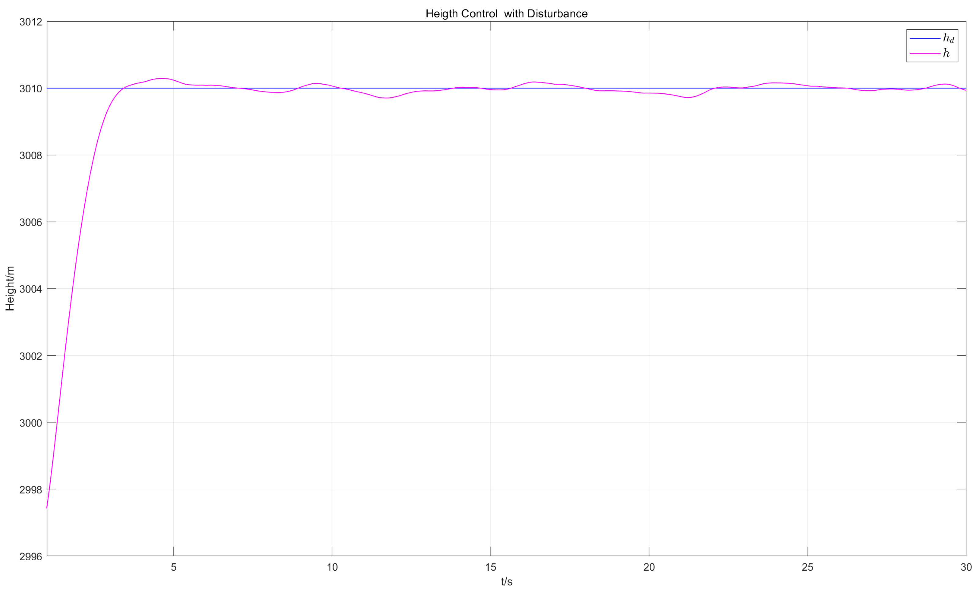
• Disturbance conditions: Initial height of $h_0=2995.4$ m, initial velocity of 197.1 m/s, and of target height $h_d=3010$ m, applying moderate-intensity Dryden turbulence wind (probability of the turbulence intensity exceeds ${10}^{-3}$) and tanker wake disturbance (acquired via computational fluid dynamics (CFD) calculations) to the receiver aircraft, using the control method proposed in this paper.
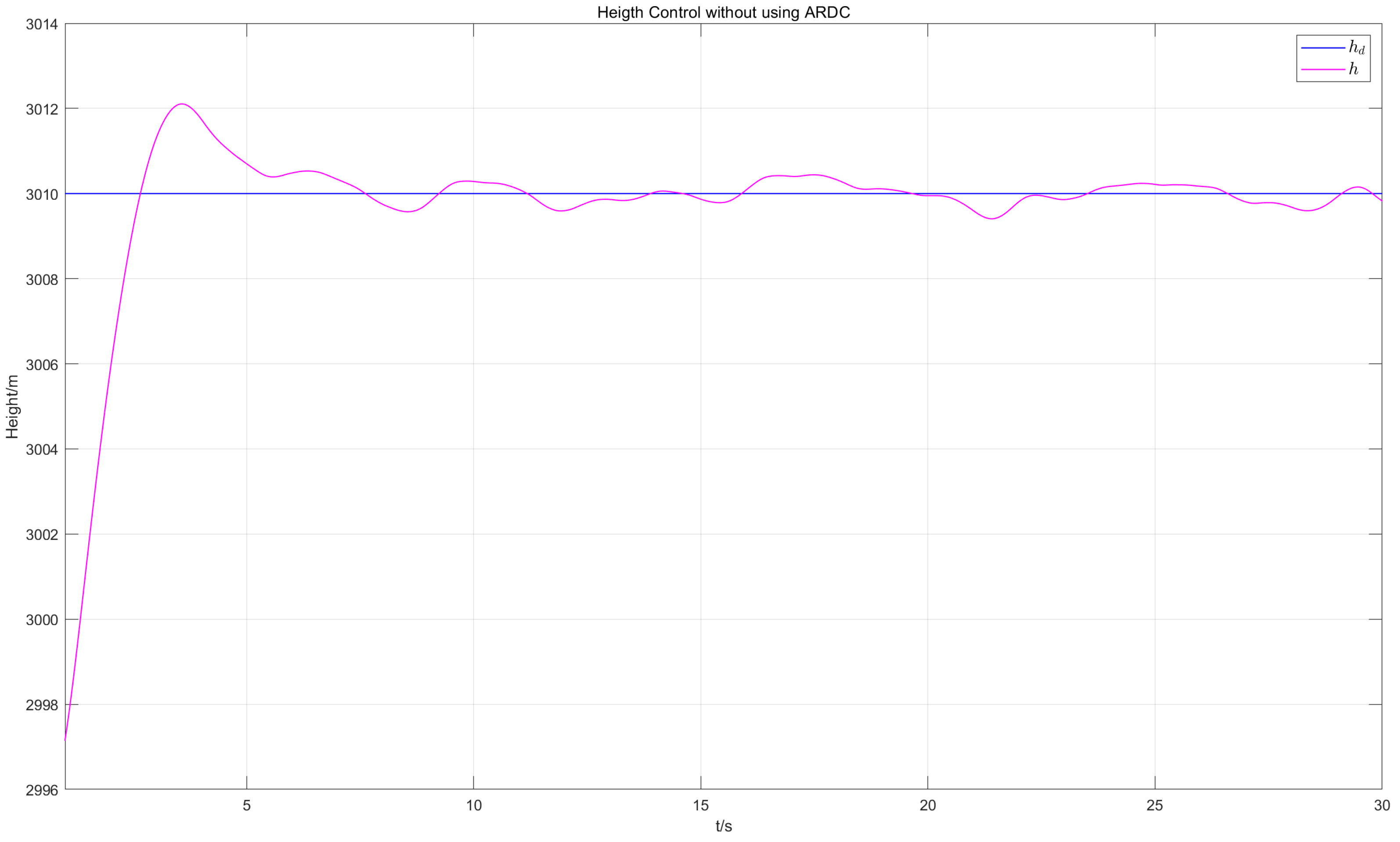
• Disturbance conditions without ARDC: Initial height of $h_0=2995.4$ m, initial velocity of 197.1 m/s, and target height of $h_d=3010$ m, applying moderate-intensity Dryden turbulence wind and tanker wake disturbance to the receiver aircraft, without using ARDC. The disturbances are the same as in scenario 2.

6.3. Analysis of Results

6.3.1. Altitude Tracking Performance

Figure 3 shows that under normal conditions, the altitude reaches the target value within 3 s, with an overshoot of no more than $2\%$ and almost no steady-state error. Figure 4 shows that when the method proposed in this paper is adopted, under disturbance conditions, the overshoot is no more than $2\%$, the maximum deviation is 0.2 m, and the system recovers stability within 3 s through compensation by the observer, verifying the robustness of the control law. Figure 5 shows that without ADRC compensation, under disturbance conditions, the overshoot reaches $20\%$ and the maximum deviation reaches 0.4 m.

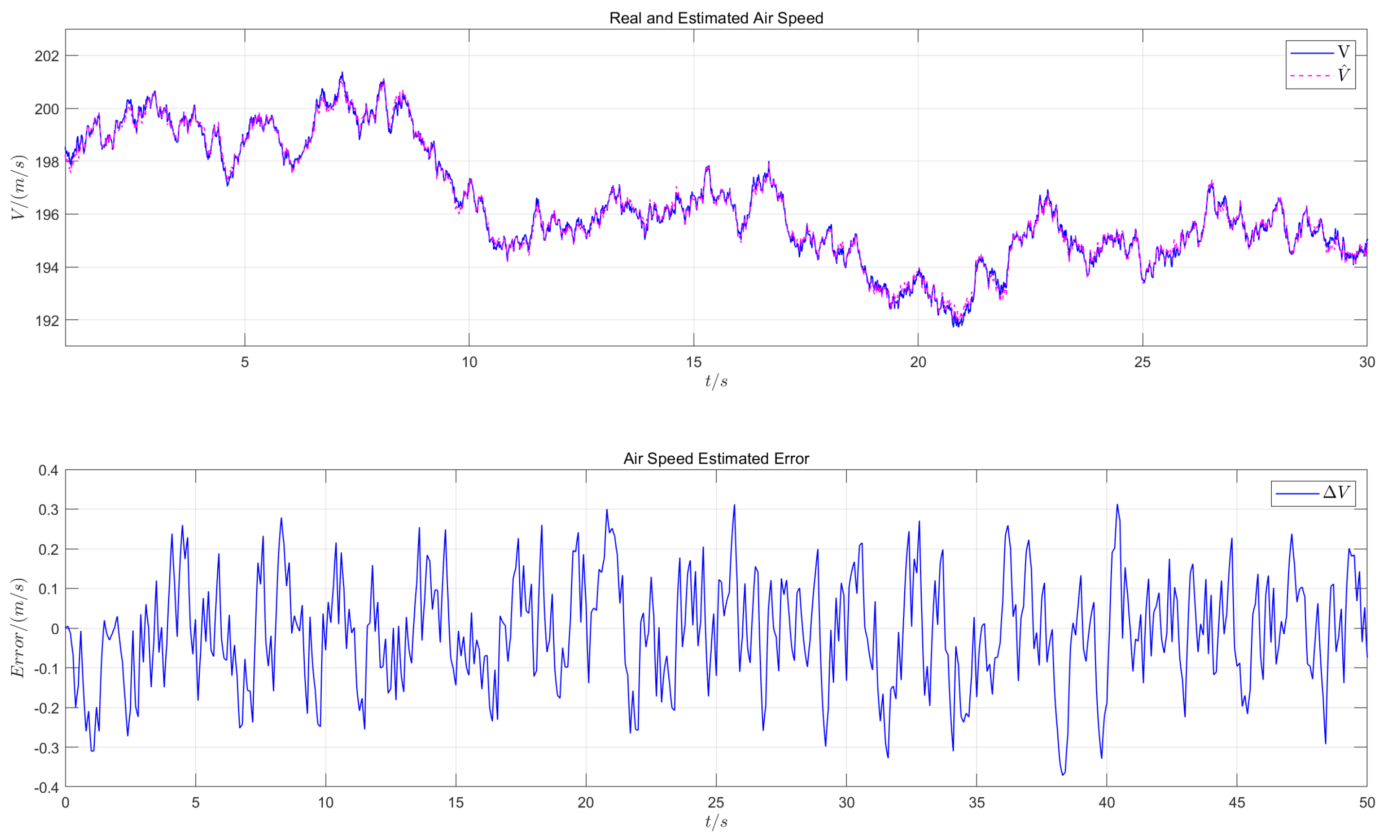
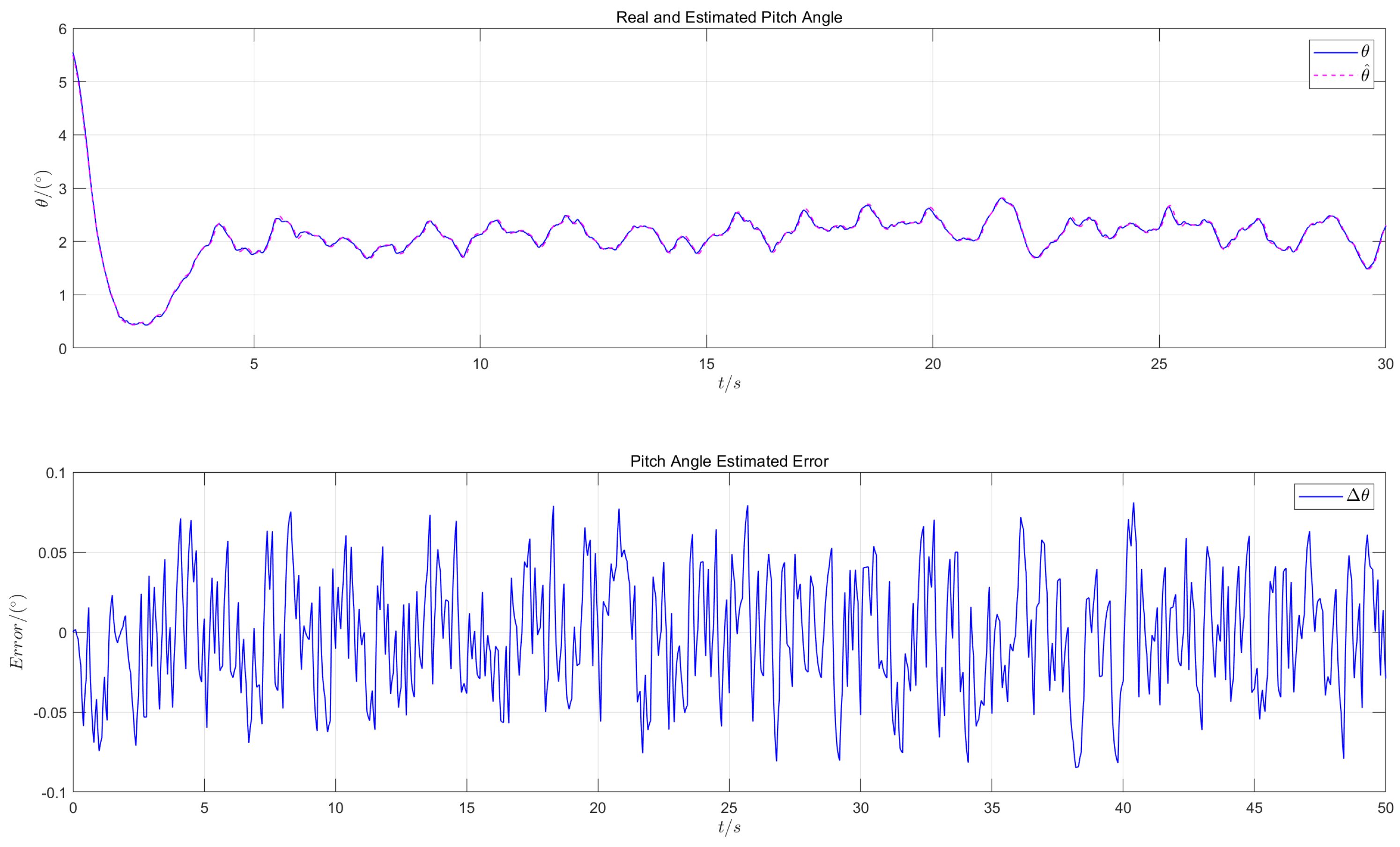
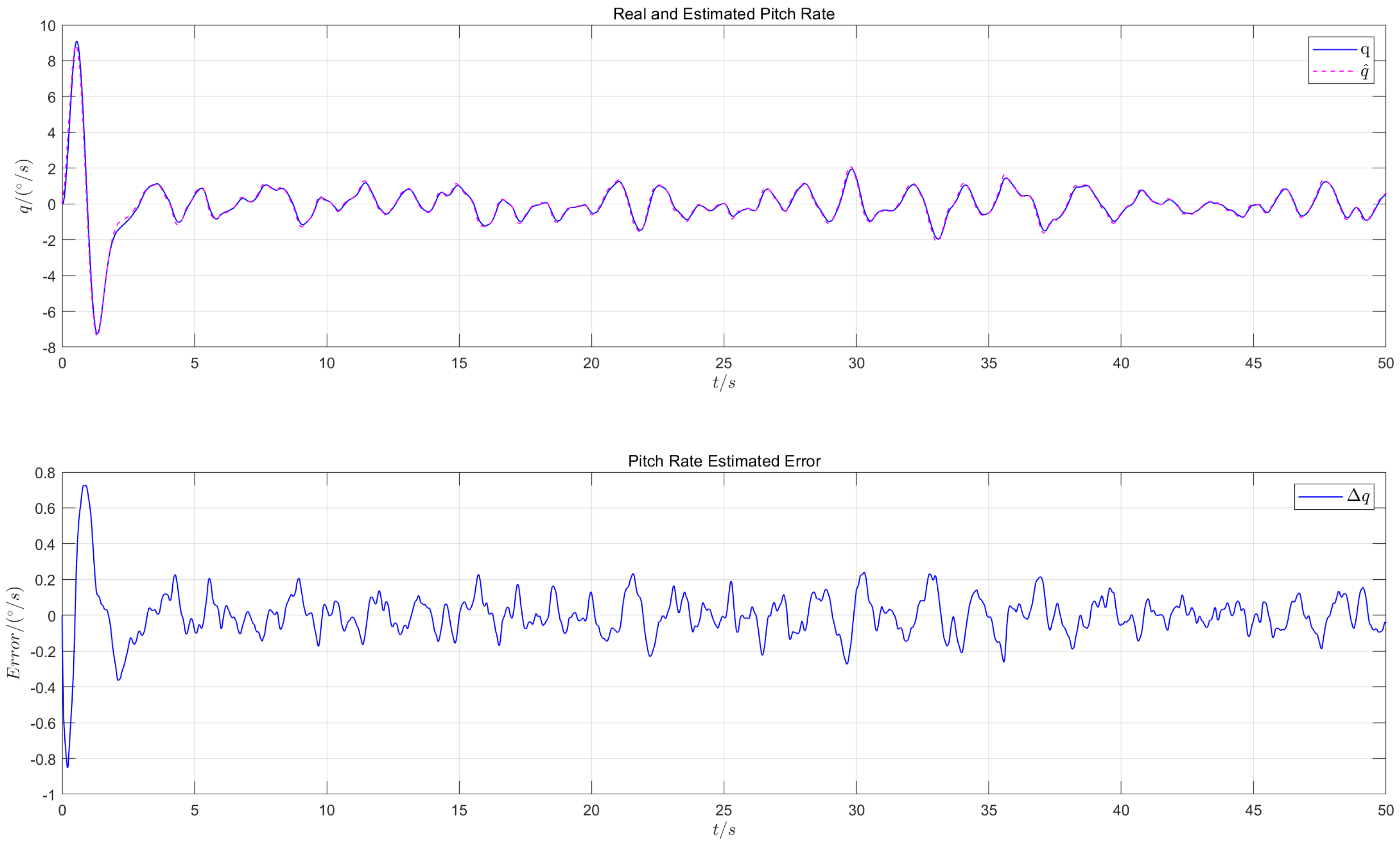
6.3.2. State Estimation Accuracy

Figure 6, Figure 7, Figure 8 and Figure 9 show that under disturbance conditions, the estimation errors of the true airspeed, angle of attack, pitch angle, and pitch rate are less than 0.3 m/s, 0.12°, 0.1°, and 0.2°/s, respectively, indicating the high-precision estimation ability of the observer.

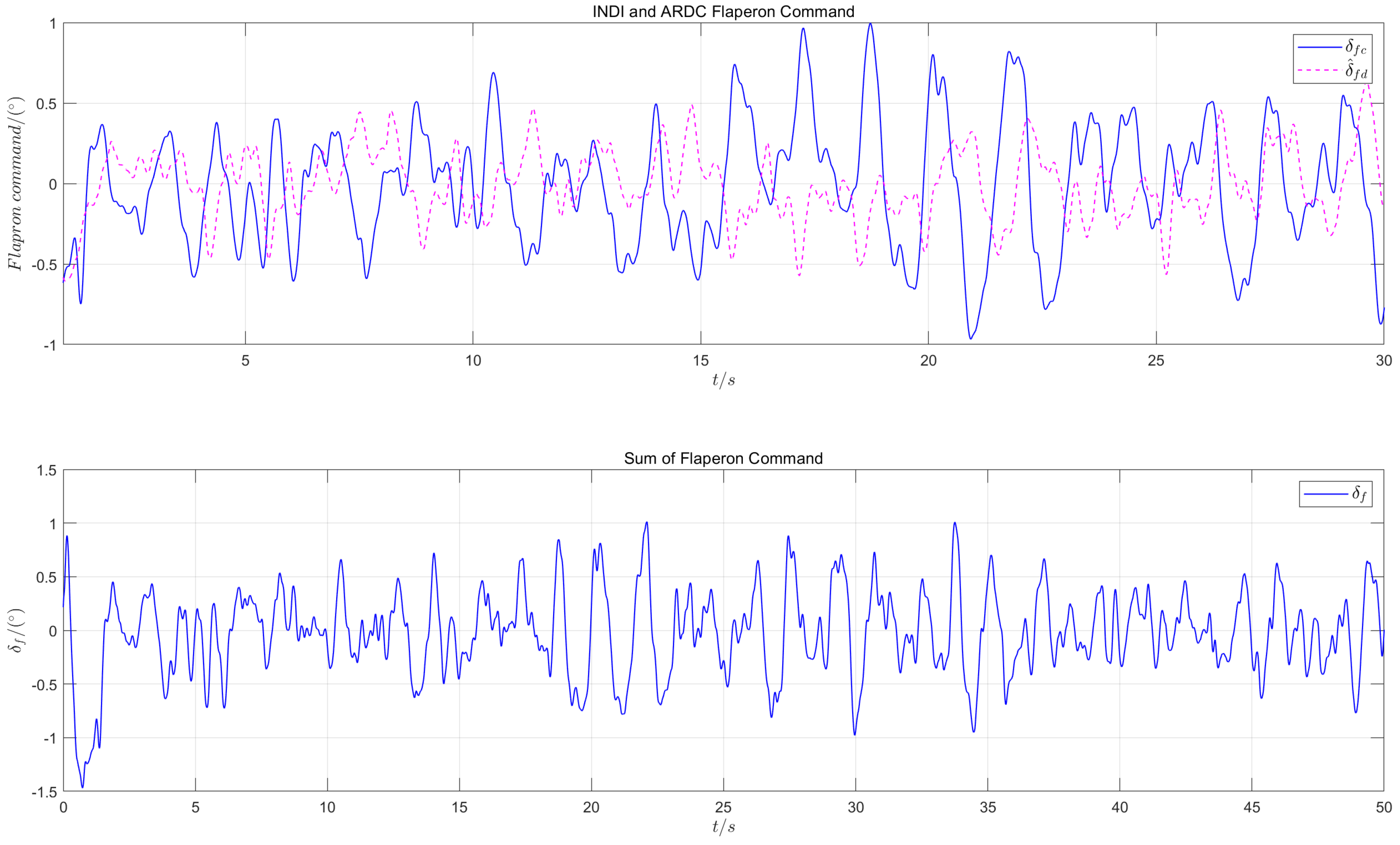
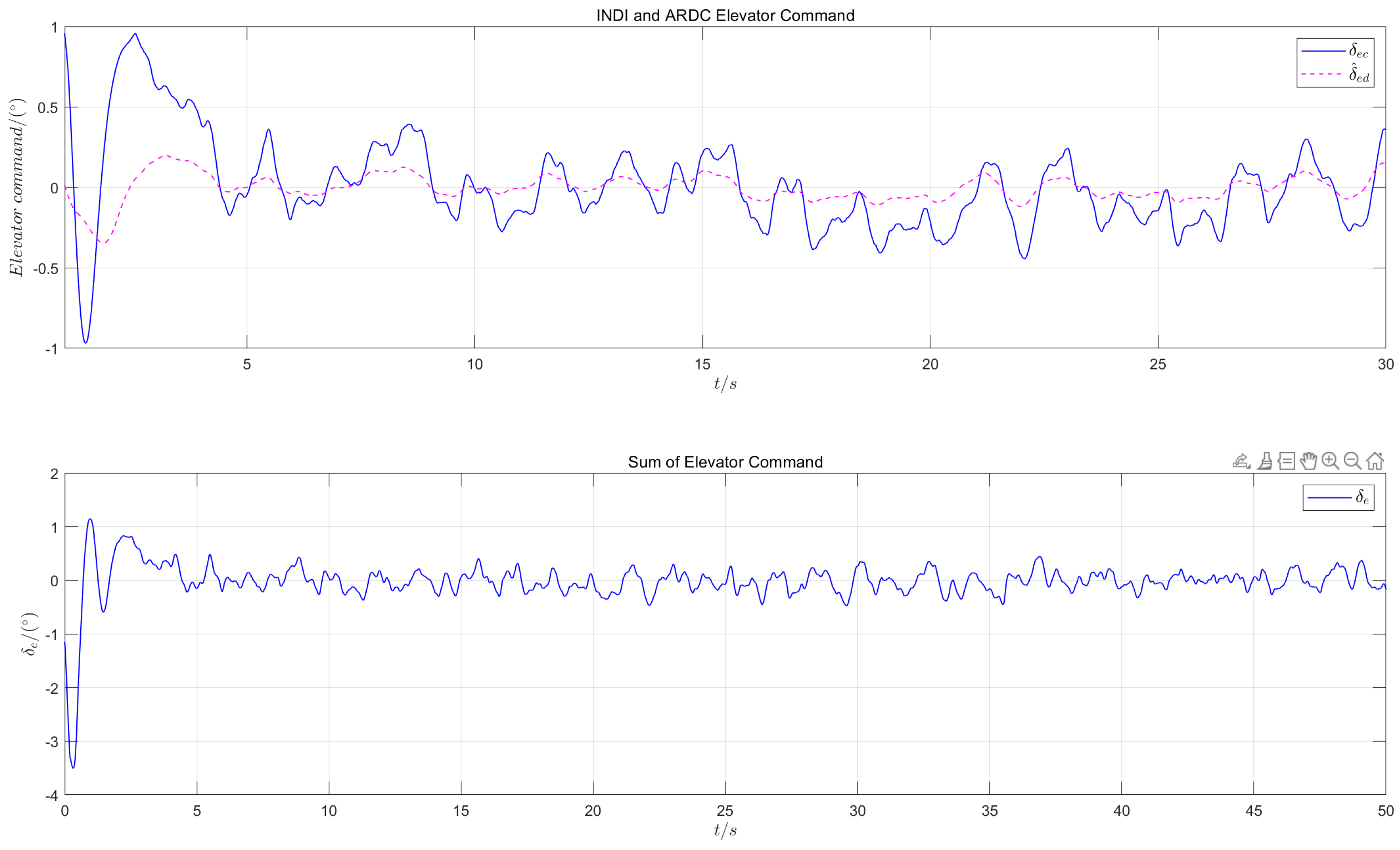
6.3.3. Characteristics of Control Surface Deflection

Figure 10 and Figure 11 illustrate that under disturbance conditions, the deflections of the control surfaces change smoothly. The maximum deflection of the flaperons is 1.5° (not exceeding the limit of ±10°), and the maximum deflection of the elevator is 3.5° (not exceeding the limit of ±20°). There is no high-frequency buffeting, meeting the safety constraints of the actuators, which demonstrates the engineering feasibility of the DLC strategy.

7. Conclusions

This paper proposes a longitudinal trajectory control strategy for the receiver aircraft that integrates DLC based on INDI with an NESO. A DLC strategy based on collaborative control of symmetric flaperons and elevators is proposed, and longitudinal dynamic equations are established. The INDI method is adopted to achieve fast tracking and control of altitude. The design approach of the NESO is presented, where observer gains are designed through pole configuration and robust enhancement optimization and the estimated disturbance forces and moments are used as control commands to effectively suppress disturbances. The Lyapunov stability theory is employed to prove the asymptotic stability of the closed-loop system. Results show that the altitude tracking error converges within 0.2 m under Dryden wind disturbances, with real-time performance and stability meeting the engineering requirements for autonomous aerial refueling of unmanned aerial vehicles.

The algorithm offers three core advantages: First, it features a fast and precise dynamic response—the DLC mechanism bypasses conventional aerodynamic delays, significantly improving the receiver aircraft’s speed in response to trajectory commands. Second, it demonstrates strong robustness—the NESO effectively estimates and compensates for internal and external system disturbances, maintaining stable tracking under moderate-intensity Dryden turbulent wind conditions. However, the algorithm has limitations: On one hand, it exhibits high a degree of model dependency, as the direct lift model requires precise matching of the receiver aircraft’s aerodynamic parameters, and airframe configuration changes during actual flight may lead to performance degradation. On the other hand, computational complexity increases significantly with the system dimension, and iterative calculations of the nonlinear observer may exceed the real-time processing capability of low-end embedded platforms when handling complex multi-input, multi-output systems.

Future research will focus on two breakthroughs: developing an adaptive parameter identification module to optimize the lift model through online learning and exploring model order reduction and distributed computing strategies to reduce algorithmic resource consumption, promoting its application in more receiver aircraft models.

References

1. Thomas, P.R.; Bhandari, U.; Bullock, S.; Richardson, T.S.; du Bois, J.L. Advances in air to air refuelling. Prog. Aerosp. Sci. 2014, 71, 14–35. [Google Scholar] [CrossRef]
2. Zhu, Y.; Sun, Y.; Zhao, W.; Huang, B.; Wu, L. Relative navigation for autonomous aerial refueling rendezvous phase. Opt.-Int. J. Light Electron Opt. 2018, 174, 665–675. [Google Scholar] [CrossRef]
3. Tao, Y.; Yan, X. Current Status and Development Trends of Foreign Aerial Refueling Technologies and Equipment. Aircr. Des. 2021, 41, 39–43. [Google Scholar]
4. Quan, Q.; Wei, Z.B.; Gao, J.; Zhang, R.F.; Cai, K.Y. A survey on modeling and control problems for probe and drogue autonomous aerial refueling at docking stage. Acta Aeronaut. Astronaut. Sin. 2014, 35, 2390–2410. [Google Scholar]
5. Ren, J.; Dai, X.; Quan, Q.; Wei, Z.; Cai, K. Reliable Docking Control Scheme for Probe–Drogue Refueling. J. Guid. Control Dyn. 2019, 42, 2511–2520. [Google Scholar] [CrossRef]
6. Li, Y.; Zhang, Y.; Bai, J. Numerical Simulation of the Aerodynamic Influence of Aircrafts During Aerial Refueling with Engine Jet. Int. J. Aeronaut. Space Sci. 2020, 21, 15–24. [Google Scholar] [CrossRef]
7. Huang, Y.; Yuan, S.; Yan, L. Aerial Refueling Docking Flight Control Based on Direct Lift. Ordnance Ind. Autom. 2021, 40, 62–67. [Google Scholar]
8. Lou, J. Research on Key Technology of Precise Control for Aerial Refueling UAV. Ph.D Thesis, Northwestern Polytechnical University, Xi’an, China, 2014. [Google Scholar]
9. Zhang, B. Docking Control Method For Autonomous Aerial Refueling For Unmanned Aerial Vehicles. Master’s Thesis, Harbin Institute of Technology, Harbin, China, 2014. [Google Scholar]
10. Wang, L.; Yin, H.; Guo, Y. Closed-loop Motion Characteristic Requirements of Receiver Aircraft for Probe and Drogue Aerial Refueling. Aerosp. Sci. Technol. 2019, 93, 105293. [Google Scholar] [CrossRef]
11. Kriel, S.C.; Engelbrecht, J.A.; Jones, T. Receptacle Normal Position Control for Automated Aerial Refueling. Aerosp. Sci. Technol. 2013, 29, 296–304. [Google Scholar] [CrossRef]
12. Hua, Y.; Zou, Q.A.; Tian, H. Control Strategy and Simulation for Probe and Drogue Aerial Autonomous Refueling. J. Beijing Univ. Aeronaut. Astronaut. 2021, 49, 262–270. [Google Scholar]
13. Wang, H.; Liu, Y.; Su, Z. Precise Docking Control for UAV Autonomous Aerial Refueling. Electron. Opt. Control 2020, 27, 1–8. [Google Scholar]
14. Wu, J.; Luo, H.; Ai, J. Docking Controller for Autonomous Aerial Refueling with Adaptive Dynamic Surface Control. IEEE Access 2020, 8, 99846–99857. [Google Scholar] [CrossRef]
15. Huang, Y. Flight Control and Simulation of Aerial Refueling Docking Based on Direct Force. Master’s Thesis, Nanjing University of Aeronautics and Astronautics, Nanjing, China, 2014. [Google Scholar]
16. Du, X.; Zhu, Z.; Hu, F.; Huang, J.; Liu, G.; Zhang, S.; Shan, E.; Tang, J. Guidance, Navigation and Control for Airborne Docking of Autonomous Aerial Refueling. Acta Aeronaut. Astronaut. Sin. 2023, 44, 628827. [Google Scholar]
17. Hernández-González, O.; Targui, B.; Valencia-Palomo, G.; Guerrero-Sánchez, M.E. Robust cascade observer for a disturbance unmanned aerial vehicle carrying a load under multiple time-varying delays and uncertainties. IEEE Syst. J. 2024, 55, 1056–1072. [Google Scholar] [CrossRef]
18. Guerrero-Sánchez, M.E.; Montoya-Morales, J.R.; Valencia-Palomo, G.; Hernández-González, O. Robust IDA-PBC for non-separable PCH systems under time-varying external disturbances. Nonlinear Dyn. 2025, 113, 3499–3510. [Google Scholar] [CrossRef]
19. Liu, Y.; Wang, H.; Fan, J. Docking Safety Assessment and Optimization for Autonomous Aerial Refueling: A Data-Driven Method. IEEE Syst. J. 2021, 15, 4057–4068. [Google Scholar] [CrossRef]
20. Yi, Y.; Zheng, W.; Liu, B. Adaptive Anti-Disturbance Control for Systems with Saturating Input via Dynamic Neural Network Disturbance Modeling. IEEE Trans. Cybern. 2022, 52, 5290–5300. [Google Scholar] [CrossRef]
21. Fravolini, M.L.; Ficola, A.; Campa, G. Modeling and Control Issues for Autonomous Aerial Refueling for UAVs Using a Probe–drogue Refueling System. Aerosp. Sci. Technol. 2004, 8, 611–618. [Google Scholar] [CrossRef]
22. Chen, H.; Zhang, S.; Fang, Z. Implicit NDI Robust Nonlinear Control Design with Acceleration Feedback. Acta Aeronaut. Astronaut. Sin. 2009, 30, 597–603. [Google Scholar]
23. Song, M.; Zhang, F.; Huang, X.; Huang, P. Anti-Disturbance Control for Tethered Aircraft System with Deferred Output Constraints. IEEE/CAA J. Autom. Sin. 2023, 10, 474–485. [Google Scholar] [CrossRef]
24. Chen, Z.; Gao, Q. Linear/nonlinear switching extended state observer. Control Theory Appl. 2019, 36, 902–908. [Google Scholar]
25. Liu, J.; Tan, J.; Li, H.; Chen, B. Active Disturbance Rejection Consensus Control of Multi-Agent Systems Based on a Novel NESO. Control Theory Appl. 2025, 30, 634–644. [Google Scholar] [CrossRef]
Figure 1. Schematic diagram of the receiver aircraft.
Machines 13 00525 g001
Figure 2. Architectural diagram of the receiver aircraft’s altitude control law.
Machines 13 00525 g002
Figure 3. Altitude tracking performance under normal conditions.
Machines 13 00525 g003
Figure 4. Altitude tracking performance under disturbance conditions (using method proposed in this paper).
Machines 13 00525 g004
Figure 5. Altitude tracking performance under disturbance conditions (without using ARDC).
Machines 13 00525 g005
Figure 6. Estimation accuracy of true airspeed under disturbance conditions.
Machines 13 00525 g006
Figure 7. Estimation accuracy of the angle of attack under disturbance conditions.
Machines 13 00525 g007
Figure 8. Estimation accuracy of the pitch angle under disturbance conditions.
Machines 13 00525 g008
Figure 9. Estimation accuracy of the pitch rate under disturbance conditions.
Machines 13 00525 g009
Figure 10. Deflection characteristics of flaperons under disturbance conditions.
Machines 13 00525 g010
Figure 11. Deflection characteristics of the elevator under disturbance conditions.
Machines 13 00525 g011