Online Tuning of Koopman Operator for Fault-Tolerant Control: A Case Study of Mobile Robot Localising on Minimal Sensor Information

Abstract

Self-localisation is a critical concept in the context of autonomous navigation and control of mobile robots. The most prevalent method for localisation is sensor fusion. Nevertheless, there are certain situations where the robots are compelled to localise on minimal sensor information. Furthermore, the key challenge is determining how to localise if this minimal sensor information fails. This paper proposes a data-driven analytical redundancy technique to address this challenge in wheeled mobile robots. Initially, the localisation of the robot is performed using the encoder information alone to create a minimalistic approach. In such a situation, a fault or failure in the encoders makes the robot behave in an undesirable way. To mitigate this, we are proposing a method to use the information from the analytical models when a fault is detected. Specifically, we obtain the analytical models through data-driven techniques. By a step response experiment, the input voltage and output angular velocity data of the motor are collected. We then use the System Identification toolbox in MATLAB^® (ver R2025a) and the Koopman framework to obtain different analytical models using the same data. We observe that these models experience errors at different input voltages of the motor, affecting the proposed method for handling the encoder fault. So, in this work, we use online tuning of the Koopman operator and experimentally demonstrate its effectiveness in handling the sensor fault on a mobile robot localising with minimal information.

1. Introduction

The superior payload capacity of autonomous wheeled mobile robots makes them applicable in a variety of industrial sectors [1], in a multi-agent collaborative environment [2], in the military for search and rescue operations in hazardous locations, and in medical applications such as autonomous wheelchairs [3]. To accomplish the task, the self-localisation of these robots plays a crucial role for autonomous navigation, guidance and control. However, these are highly susceptible to onboard sensor faults, which have an immediate impact on their autonomous trajectory tracking capabilities [4]. Therefore, it is crucial for the robot to be able to tolerate these faults in such critical applications.

1.1. Related Works

1.1.1. Sensor Fault-Tolerant Localisation of Mobile Robot

The literature extensively discusses sensor fault detection and fault-tolerant control strategies for mobile robot localisation. In [5] a sensor fault-tolerant architecture is developed using multisensor data fusion with a Kalman filter approach on a real car. Another approach to fault-tolerant localisation is presented in [6], where sensor data are fused in alternating pairs using Extended Kalman Filters (EKF). By comparing the outputs of the fusion processes, the authors demonstrate effective fault tolerance on an autonomous mobile robot. In [7], the authors developed a fault-tolerant sensor fusion scheme to address the limitations of single-sensor-based localisation, such as hardware/software failures or sudden data outages. Their method fuses the sensor information from two onboard IMUs (Inertial Measurement Units) and wheel encoders using Interacting Multiple Model Kalman filters (IMM). Similarly, in [8] the LiDAR sensor faults are detected, and fault tolerance is achieved by fusing wheel encoder and IMU information using EKF. In another study [9], a nonlinear information filter is used to tightly fuse the GNSS (Global Navigation Satellite System) and IMU data to obtain fail-safe vehicle localisation. Indeed, there are many other studies that adopt sensor fusion for fault-tolerant localisation of the robot [10,11,12]. While sensor fusion-based fault-tolerant schemes are robust and reliable, there are specific scenarios in which sensor capabilities are constrained, such as GNSS/GPS-denied locations [13,14], poor and indistinct camera vision [15], IMU calibration inaccuracies and drifting errors [16], and encoder malfunctions. So, the robot is compelled to localise on minimal sensor information in such unavoidable cases. Furthermore, the key challenge is how to localise if this minimal sensor information fails. To address this, Ref. [17] presents the system identification approach of a whole vehicle model by considering intermittent loss of self-localisation. Then, it uses the information from the identified vehicle model in combination with vehicle dynamics to handle this intermittent loss. However, the work is limited to only intermittent faults and is validated through simulations. To our knowledge, the fault-tolerant control of a mobile robot considering the complete failure of the minimal sensor information required for localisation is not studied in the literature.

Physical redundant sensors can mitigate the malfunctions, although at the expense of additional costs and space, but cannot entirely eliminate them [18]. Moreover, if the number of faulty sensors is more than the normal sensors, the overall decision is not reliable [19] and increases the risk of system failure [6]. Then there is analytical redundancy, which employs a mathematical or analytical model to mitigate the drawbacks of physical redundancy [20]. Typically, the analytical models are popular in fault detection and isolation (FDI) techniques [21]. In contrast, this work focuses on using it for fault-tolerant control (FTC).

1.1.2. Koopman Framework Based Control of Autonomous Systems

The analytical models are mathematical equations describing the dynamics, or input-output behaviour, of the system [22]. The parameters in this set of dynamical equations are responsible for predicting the accurate output. However, due to ageing effects, wear and tear, etc., these parameters change with time, affecting the accuracy of predictions. Data-driven techniques, which identify the analytical models purely from the data, can effectively handle these variations [23]. The Koopman framework is one such data-driven mathematical framework that identifies the dynamical model of a nonlinear system as a higher-dimensional linear system which is valid over a wide range [24,25]. This approach of handling the nonlinear systems as higher-dimensional linear systems offers advantages to use the well-developed linear control techniques over alternative data-driven techniques [26]. Koopman initially proposed the concept of the framework [27], which subsequently garnered increased interest as a data-driven methodology in control systems [28,29]. Many researchers have employed it for the data-driven identification and control of autonomous systems [30,31,32,33,34]. Recently, its implementation has been extended to fault detection and identification in autonomous systems like manipulators [35] and quadrotors [36]. Motivated by its successful implementation in the literature, this work leverages this framework and investigates it in handling the abrupt encoder fault in the closed-loop control of a Direct Current (DC) motor. Although, in a previous work, the Koopman framework is applied to the DC motor [37], our study extends its scope to physical implementation and fault-tolerant control.

Building on these insights, this work addresses the critical problem of complete loss of minimal sensor information for localisation. Unlike existing approaches that rely on sensor fusion, this study explores the deployment of a Koopman-based linear model for fault-tolerant control. Furthermore, we incorporate the online tuning of the Koopman operator to enhance the experimental performance. For benchmarking purposes, a widely used data-driven technique from MATLAB^® System Identification Toolbox is taken into consideration [38,39].

The main contributions of the work are summarised as follows:

• Data-driven Koopman framework-based fault-tolerant localisation: While the sensor fusion provides a reliable and robust localisation [7,8], the capabilities of sensors are limited in challenging scenarios [13,16]. Addressing the challenge where even minimal sensor information for localisation fails, this study adopts the Koopman operator framework to achieve fault-tolerant localisation. The Koopman framework-based data-driven model of the DC motor is identified and leveraged in the Koopman-based linear observer to detect and compensate for the encoder sensor faults.
• Extension of the Koopman framework to fault-tolerant control: In contrast to previous studies that deployed the Koopman framework for identification and control of autonomous systems [30,31,32,33,34,36], this work extends its application to fault-tolerant control. Furthermore, the online tuning of the Koopman operator is implemented for efficient fault-tolerant trajectory tracking.

1.2. Overview of the Problem Statement

This work assumes that the robot fully relies on the wheel encoder’s information for self-localisation and trajectory tracking. During tracking, an abrupt sensor fault occurs, resulting in the complete loss of information from one of the encoders. Consequently, the robot is unable to localise itself in the inertial frame, and the angular velocity of the wheel cannot be regulated in the closed loop, which has a direct impact on the robot’s trajectory tracking. This study aims to address this issue by using auxiliary sensor readings derived from the data-driven analytical models of the DC motor in the event of a fault. We used the DC motor’s input voltage-output angular velocity data to determine these analytical models by two data-driven methodologies: the System Identification toolbox in MATLAB^® and the Koopman Framework. We also discuss an online tuning method for the Koopman operator to improve the result.

The rest of the paper is organised as follows. Section 2 gives a brief description of the Koopman framework and the System Identification Toolbox of MATLAB^®. Section 3 describes the wheeled robot used in the experiment and its trajectory tracking. Section 4 delves into the development of analytical models and their implementation for FDI and FTC. Section 5 discusses the results and Section 6 concludes the work, discussing the future works.

2. Preliminaries

2.1. Koopman Framework

The Koopman operator [24] can handle nonlinear systems with a globally linear description. The Koopman operator is briefly explained here (see [40] for a more thorough explanation). Consider a nonlinear system (here: a DC motor) with state $w_x\in R^n$ and input $u\in R^r$.

$$\begin{array}{cc}\hfill {\dot{w}}_x& =\mathbf{f}(w_x,u)\hfill \end{array}$$

(1)

The state $w_x\in R^n$ in the nonlinear system (1) propagates over time by a nonlinear map $\mathbf{f}:R^n\times R^r\to R^n$. Furthermore, there is a set of scalar-valued functions $g\in \mathcal{H}$ referred to as observable functions. These functions, which belong to the infinite-dimensional Hilbert space, $\mathcal{H}$ are dependent on the states and inputs. A linear, infinite-dimensional Koopman operator $\mathcal{K}:\mathcal{H}\to \mathcal{H}$ is given as follows:

$$\begin{array}{cc}\hfill \mathcal{K}g(w_x,u)& =g\left(\mathbf{f}(w_x,u)\right)\hfill \end{array}$$

(2)

Unlike (1), the observable functions g are linearly evolved over time using this operator $\mathcal{K}$. However, in practice, a finite-dimensional Koopman operator, K is approximated. Figure 1 shows the illustration of obtaining a finite-dimensional Koopman operator. At a specific sampling time, $m+1$ time-domain samples of the state data $w_x\in R^n$ and input data $u\in R^r$ are collected from a given nonlinear dynamical system (1). The collected data are then arranged in the sets: $U\in R^{r\times m}$, $W_x\in R^{n\times m}$ and $W_y\in R^{n\times m}$. U is referred to as the input data matrix and $W_x$, $W_y$ as the state data matrix. Furthermore, $W_y$ is the left-shifted data matrix of $W_x$ by one instant, such that $w_y\left(k\right)=w_x(k+1)$ with $w_y\left(k\right)\in W_y$ and $w_x(k+1)\in W_x$. Using observable functions $g={[g_1,g_2...,g_p]}^T$; $g_i:R^n\to R$, these collected data matrices $W_x$ and $W_y$ are lifted to $Z_X$ and $Z_Y$, with each element as $z_x\left(k\right)=g\left(w_x\left(k\right)\right)$, $w_x\left(k\right)$ being the $k^{th}$ sample. These scalar-valued observable functions are selected either as physics-inspired observable functions with strong knowledge of the dynamics or by adopting machine learning techniques. Finally, an optimisation problem,

$$\begin{array}{cc}\hfill \underset{A,B}{min}& \left|\right|Z_Y-A{Z}_X-BU{\left|\right|}_F\hfill \\ \hfill \underset{C}{min}& \left|\right|W_x-C{Z}_X{\left|\right|}_F\hfill \end{array}$$

(3)

as shown in (3), is solved to obtain the approximated Koopman operator $K=\left[\begin{array}{cc}A& B\end{array}\right]$. Using C, the original states are deduced from the lifted states. Thus, a Koopman linear model with state and input matrices, respectively, as $A\in R^{p\times p}$,$B\in R^{p\times r}$ and an output matrix $C\in R^{n\times p}$ is obtained. The Koopman linear state space form is given as

$$\begin{array}{cc}\hfill z_x(k+1)& =A{z}_x\left(k\right)+Bu\left(k\right)\hfill \\ \hfill w_x\left(k\right)& =C{z}_x\left(k\right)\hfill \end{array}$$

(4)

where $z_y\left(k\right)=g\left(w_y\left(k\right)\right),z_x\left(k\right)=g\left(w_x\left(k\right)\right),u\left(k\right)\in U$. The minimisation problem (3) is solved analytically as follows to obtain the Koopman predictor matrices († denotes the pseudo-inverse).

$$\begin{array}{cc}\hfill K=\left[\begin{array}{cc}A& B\end{array}\right]& =M\ast G^{†}\hfill \\ \hfill whereM& ={\displaystyle \frac{1}{m+1}}\sum _{k=1}^m{z}_y\left(k\right)\ast {\left[\begin{array}{c}{z}_x\left(k\right)\\ u\left(k\right)\end{array}\right]}^T\hfill \\ \hfill G& ={\displaystyle \frac{1}{m+1}}\sum _{k=1}^m\left[\begin{array}{c}{z}_x\left(k\right)\\ u\left(k\right)\end{array}\right]\ast {\left[\begin{array}{c}{z}_x\left(k\right)\\ u\left(k\right)\end{array}\right]}^T\hfill \\ \hfill C=N\ast H^{†}\\ \hfill whereN& ={\displaystyle \frac{1}{m+1}}\sum _{k=1}^m{w}_x\left(k\right)\ast {\left[\begin{array}{c}{z}_x\left(k\right)\end{array}\right]}^T\hfill \\ \hfill H& ={\displaystyle \frac{1}{m+1}}\sum _{k=1}^m\left[\begin{array}{c}{z}_x\left(k\right)\end{array}\right]\ast {\left[\begin{array}{c}{z}_x\left(k\right)\end{array}\right]}^T\hfill \end{array}$$

(5)

2.2. Transfer Function Estimation by System Identification Toolbox of MATLAB^®

The system identification toolbox in MATLAB^® estimates a transfer function from the measured input ‘$u\left(t\right)$’-output ‘$w_x\left(t\right)$’ time domain data of a system. Considering $U\left(s\right)$ and $W\left(s\right)$ as the Laplace transforms of input and output variables, the general transfer function model of a Single Input–Single Output (SISO) system is given as

$$\begin{array}{c}\hfill G={\displaystyle \frac{W\left(s\right)}{U\left(s\right)}}={\displaystyle \frac{a_z{s}^{n_z}+a_{z-1}{s}^{n_z-1}+...+a_0{s}^0}{b_p{s}^{n_p}+b_{p-1}{s}^{n_p-1}+...+1}}\end{array}$$

(6)

The transfer function G is ‘Proper’ and has $n_z$ zeros and $n_p$ poles ($n_p\ge n_z$). The model parameters $\alpha ={[a_z,a_{z-1},..,a_0,b_p,b_{p-1},..,b_1]}^T$ in (6) are unknown. These model parameters ‘$\alpha$’ should be estimated in such a way that the error between the predicted output and measured output is as small as possible. The Nonlinear Least Squares algorithm is used by the toolbox to estimate the parameters. The flow of the estimation procedure is shown in Figure 2.

Consider ‘m’ time domain data samples are collected and arranged into an output data matrix $W_x\in R^{1\times m}$ and an input data matrix $U\in R^{1\times m}$. Initialising the model parameters (MATLAB^® generally uses the ‘Instrumental Variables (IV)’ method [41]), the output $W_{pred}\in R^{1\times m}$ is predicted as follows:

$$\begin{array}{cc}\hfill W_{pred}& =G\left(\alpha \right)U\hfill \\ \hfill V& =W_x^T-W_{pred}^T\hfill \\ \hfill J\left(\alpha \right)& =V^{T}V\hfill \end{array}$$

(7)

The objective is to minimise the cost function $J\left(\alpha \right)$, which is the sum of squared errors or the inner product of the error vector $V\in R^m$. To minimise it, the parameters ‘$\alpha$’ are iteratively updated as

$$\begin{array}{c}\hfill \alpha +=\Delta \alpha \end{array}$$

until convergence. The $\Delta \alpha$ can generally be found by solving the following linear equation based on the Gauss–Newton algorithm [42]:

$$\begin{array}{cc}\hfill \left({\mathbf{J}}^T\mathbf{J}\right)\Delta \alpha & =-{\mathbf{J}}^{T}V\hfill \\ \hfill \mathrm{with}{j}_{ij}& ={\displaystyle \frac{\partial V\left(i\right)}{\partial \alpha \left(j\right)}}\in \mathbf{J}\hfill \end{array}$$

where $\mathbf{J}$ is the Jacobian matrix, in which each element $j_{ij}$ shows the sensitivity of the $i^{th}$ residual $V\left(i\right),i\in [1,m]$ with respect to the $j^{th}$ parameter $\alpha \left(j\right),j\in [1,(n_p+n_z+1)]$. As shown in Figure 2, the above procedure is repeated until convergence. The criteria for convergence is $\Delta \alpha <ϵ$, where $ϵ$ will be a small value, implying that the parameters of the transfer function G are estimated. MATLAB^® provides a direct command $tfest$ to estimate the transfer function [41] using the above procedure.

3. Trajectory Tracking of Wheeled Robot

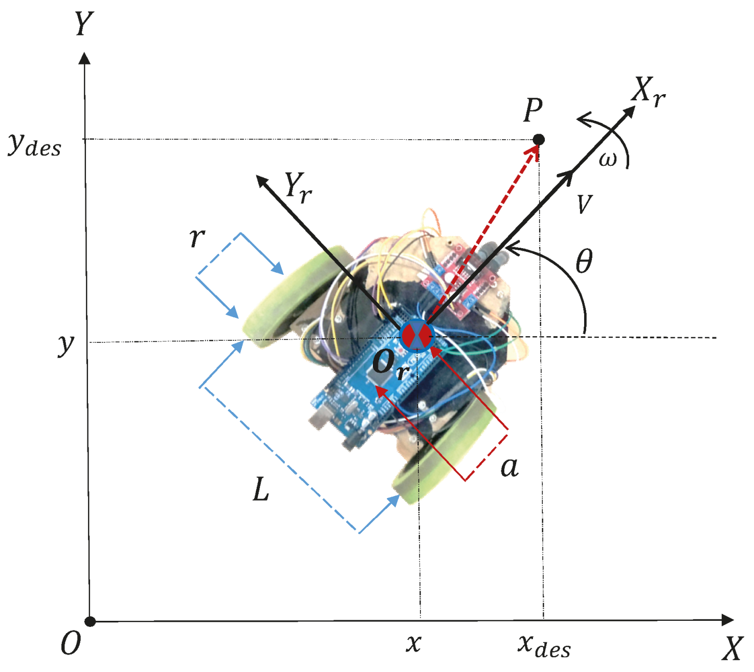
3.1. Description of Wheeled Robot

A three-wheeled robot is used in the work. As shown in Figure 3, it consists of two active rear wheels, each controlled by a DC motor with an encoder, and a passive wheel in the front. $X-O-Y$ and $X_r-O_r-Y_r$ represent the inertial frame and robot frame, respectively. The robot’s linear velocity and angular velocity in the robot frame are given by V and $\omega$, respectively. r is the radius of the wheel, and L is the distance between the centres of the two wheels. a refers to the distance between the centre of the robot and the centre of the line that connects the two wheels. $\theta$ is the angle of the robot frame with respect to the inertial frame. ${[x,y]}^T$ is the current position of the robot, ${[\dot{x},\dot{y}]}^T$ are the velocities, and $\dot{\theta }$ is the angular velocity of the robot in the inertial frame. $w_r$ and $w_l$ represent the right and left wheel angular velocities.

The DC motors are rated at $260 \mathrm{RPM}$ and $12 \mathrm{V}$, with a magnetic encoder sensor attached to their shaft. The physical parameters $r,L,a$ of the robot are $5 \mathrm{cm}$, $17.5 \mathrm{cm}$, and $5 \mathrm{cm}$, respectively. A motor driver L298N connected to an Arduino Mega 2560 is used to control the speed of the motors.

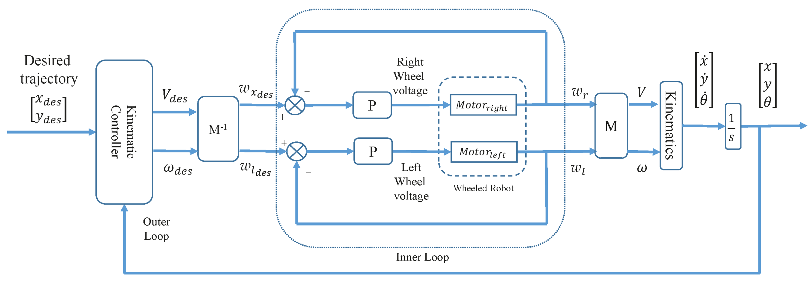
3.2. Trajectory Tracking

The forward kinematics of the two-wheeled robot are given by

$$\begin{array}{cc}\hfill V& =r{\displaystyle \frac{(w_r+w_l)}{2}}\hfill \\ \hfill \omega & =r{\displaystyle \frac{(w_r-w_l)}{L}}\hfill \end{array}$$

(8)

where the inverse kinematics are

$$\begin{array}{cc}\hfill \left[\begin{array}{c}{w}_r\\ w_l\end{array}\right]& =M^{-1}\left[\begin{array}{c}V\\ \omega \end{array}\right]\hfill \\ \hfill \mathrm{such}\mathrm{that}M& =\left[\begin{array}{cc}r/2& r/2\\ r/L& -r/L\end{array}\right]\hfill \end{array}$$

(9)

The velocities in the inertial frame are given by the standard transformation from the robot frame as follows:

$$\begin{array}{cc}\hfill \dot{x}& =Vcos\theta -a\omega sin\theta \hfill \\ \hfill \dot{y}& =Vsin\theta +a\omega cos\theta \hfill \\ \hfill \dot{\theta }& =\omega \hfill \end{array}$$

(10)

Considering the desired position of the robot as ${[x_{des},y_{des}]}^T$ in the inertial frame, the main objective of trajectory tracking can be given mathematically as follows:

$$\begin{array}{c}\hfill \underset{t\to \infty }{lim}\left|\right|x_{des}\left(t\right)-x\left(t\right)\left|\right|\to 0\\ \hfill \underset{t\to \infty }{lim}\left|\right|y_{des}\left(t\right)-y\left(t\right)\left|\right|\to 0\end{array}$$

(11)

To achieve (11), the control law is designed for the robot, as per Figure 4. To calculate $V_{des},{\omega }_{des}$, the Kinematic controller is adopted from [3]

$$\begin{array}{c}\hfill \left[\begin{array}{c}{V}_{des}\\ {\omega }_{des}\end{array}\right]=\left[\begin{array}{cc}cos\theta & sin\theta \\ -{\displaystyle \frac{1}{a}}sin\theta & {\displaystyle \frac{1}{a}}cos\theta \end{array}\right]\left[\begin{array}{c}\dot{x}+l_{x}tanh\left({\displaystyle \frac{k_x}{l_x}}(x_{des}-x)\right)\\ \dot{y}+l_{y}tanh\left({\displaystyle \frac{k_y}{l_y}}(y_{des}-y)\right)\end{array}\right]\end{array}$$

(12)

$k_x>0,k_y>0$ are the controller gains and $l_x\in R,l_y\in R$ are the saturation constraints, which can be tuned to achieve efficient trajectory tracking. From the obtained values of $V_{des},{\omega }_{des}$ the desired right wheel $\left(w_{r_{des}}\right)$ and left wheel $\left(w_{l_{des}}\right)$ angular velocities are calculated as per inverse kinematics shown in (9). A proportional controller with gain $k_p$ is used for the DC motors in the inner loop to regulate the desired angular wheel speed. The encoders are used to obtain feedback on the angular speed. Again, following the kinematics (8), the linear velocity (V) and angular velocity ($\omega$) are calculated. Finally, the position of the robot in the inertial frame is derived from (10) and is given as feedback to the outer loop trajectory controller. Using the Ziegler–Nichols method, the motor controller gain $k_p=3$ is selected, and the values of $k_x=k_y=2.5$ and $l_x=l_y=0.1$ are tuned heuristically.

4. Development and Implementation of Analytical Models of DC Motor

This work derives three analytical models for comparison. Two state space models based on the Koopman framework and another transfer function model using the system identification toolbox in MATLAB^® are found from the same time domain data. To obtain the data, the step response experiment is performed, where the DC motor is stimulated with a voltage step input for T seconds. The $m+1$ time-domain data of output angular velocity and input voltage are collected at a sampling time of $t_s$ seconds. The obtained angular velocity data are rearranged into state matrices $W_x=[w_x\left(1\right),w_x\left(2\right),\dots ,w_x\left(m\right)]\in R^{1\times m}$ and $W_y=[w_x\left(2\right),w_x\left(3\right),\dots ,w_x(m+1)]\in R^{1\times m}$, in which the data points $w_y\left(k\right)\in W_y$ are just the time-shifted points of $w_x\left(k\right)\in W_x$ by one instant, such that $w_y\left(k\right)=w_x(k+1)$ at $k^{th}$ instant. The input data matrix is obtained with its first m data points as $U=[u\left(1\right),u\left(2\right),\dots ,u\left(m\right)]\in R^{1\times m}$. Below, we explain how to obtain the analytical models using both data-driven techniques.

4.1. System Identification Toolbox in MATLAB^®

As discussed in Section 2.2, the system identification toolbox in MATLAB^® identifies the transfer function of the system using its input and output data [38,39]. Using these data, the transfer function of the DC motor is obtained using the following MATLAB^® commands:

$$\begin{array}{cc}\hfill \mathrm{data}& =\mathrm{iddata}(W_x^T,U^T,t_s)\hfill \\ \hfill \mathrm{tf}& =tfest(\mathrm{data},n_p,n_z)\hfill \end{array}$$

(13)

The command $tfest$ estimates the transfer function (tf) with $n_p$ poles and $n_z$ zeros. The general transfer function of the DC motor is second-order with two poles. So, the transfer function is estimated with 2 poles ($n_p=2,n_z=0$) at a sampling time of $t_s(=0.02 \mathrm{s})$, using the obtained angular velocity data($W_x$) and voltage data(U).

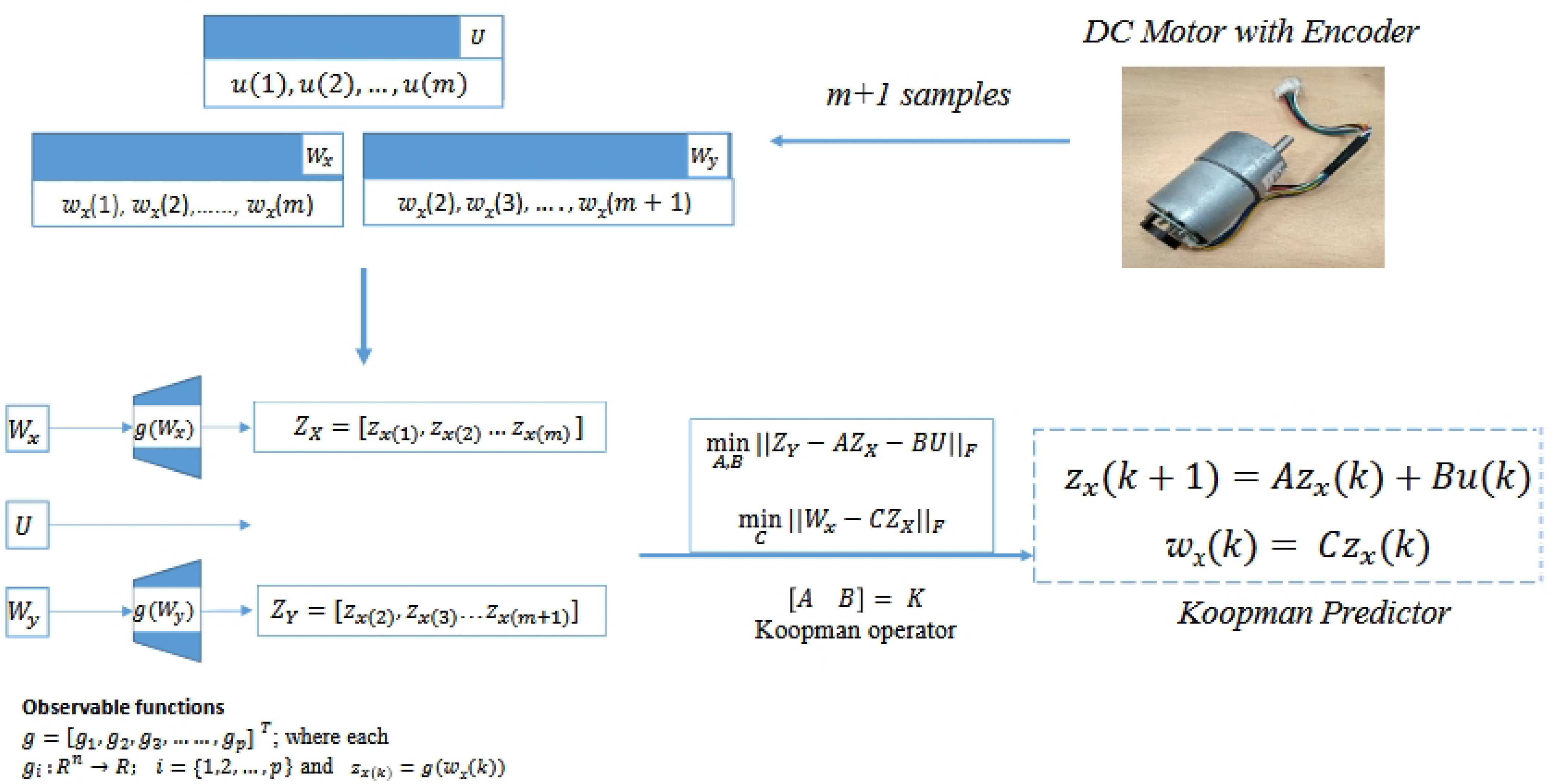
4.2. Koopman Framework

4.2.1. Dynamic Mode Decomposition

The Dynamic Mode Decomposition (DMD) is an algorithm of the Koopman framework, where the states of the system are directly considered as observable functions without the need for lifting, i.e., $z_y\left(k\right)=w_y\left(k\right),z_x\left(k\right)=w_x\left(k\right)$. As the DC motor is almost a linear system, the DMD algorithm is considered in this work. So, (5) simplifies as below to find the Koopman predictor matrices († denotes the pseudo-inverse).

$$\begin{array}{cc}\hfill K=\left[\begin{array}{cc}A& B\end{array}\right]& =M\ast G^{†}\hfill \\ \hfill whereM& ={\displaystyle \frac{1}{m+1}}\sum _{k=1}^m{w}_y\left(k\right)\ast {\left[\begin{array}{c}{w}_x\left(k\right)\\ u\left(k\right)\end{array}\right]}^T\hfill \\ \hfill G& ={\displaystyle \frac{1}{m+1}}\sum _{k=1}^m\left[\begin{array}{c}{w}_x\left(k\right)\\ u\left(k\right)\end{array}\right]\ast {\left[\begin{array}{c}{w}_x\left(k\right)\\ u\left(k\right)\end{array}\right]}^T\hfill \end{array}$$

(14)

The resultant Koopman linear predictor (denoted as DMD) is

$$\begin{array}{cc}\hfill w_x(k+1)& =A{w}_x\left(k\right)+Bu\left(k\right)\hfill \end{array}$$

(15)

The matrix C of the Koopman predictor is an identity matrix ($C=1$), as $z_x\left(k\right)=w_x\left(k\right)$.

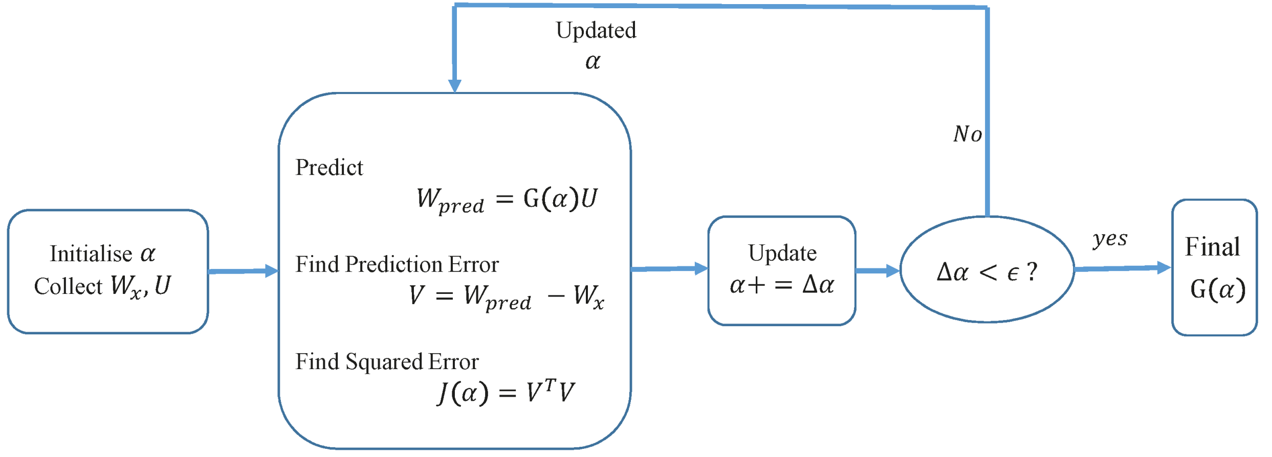
4.2.2. Online Tuning of Koopman Predictor

From the step response experiments at different input voltages, a considerable deviation in the B matrix is found, whereas the A matrix remained almost constant, as seen in Figure 5. See

Table A1. Variation in DMD-based A and B matrices for different step input experiments.

Input (Volts)	A	B
2	0.936	1.355
3	0.934	1.382
4	0.929	1.463
5	0.928	1.488
6	0.928	1.467
7	0.93	1.432
8	0.931	1.408
9	0.931	1.411
10	0.932	1.367
11	0.932	1.369
12	0.931	1.363

for the DMD-based Koopman operators for step response experiments at different input voltages.

So, fixing the A matrix, the input matrix B of the Koopman predictor is tuned online with the last 10 instants of data, as below:

$$\begin{array}{cc}\hfill & \underset{B}{min}\left|\right|W_y-A{W}_x-BU{\left|\right|}_F^2\hfill \\ \hfill \Rightarrow & {\nabla }_B={\displaystyle \frac{\partial }{\partial B}}\left|\right|W_y-A{W}_x-BU{\left|\right|}_F^2=0\hfill \\ \hfill \Rightarrow & -2(W_y-A{W}_x-BU)U^T=0\hfill \\ \hfill \Rightarrow & (W_y{U}^T-A{W}_x{U}^T-BU{U}^T)=0\hfill \\ \hfill \Rightarrow & B=(W_y-A{W}_x)U^T{\left(U{U}^T\right)}^{-1}\hfill \end{array}$$

(16)

$$\begin{array}{cc}\hfill \therefore B\left(k\right)& =(W_{yp}-A{W}_{xp})U_p^T{\left(U_p{U}_p^T\right)}^{-1}\hfill \\ \hfill \mathrm{where}{W}_{yp}& =\left[\begin{array}{cccc}{w}_x(k-1)& w_x(k-2)& ....& w_x(k-10)\end{array}\right]\hfill \\ \hfill W_{xp}& =\left[\begin{array}{cccc}{w}_x(k-2)& w_x(k-3)& ....& w_x(k-11)\end{array}\right]\hfill \\ \hfill U_p& =\left[\begin{array}{cccc}u(k-2)& u(k-3)& ....& u(k-11)\end{array}\right]\hfill \end{array}$$

(17)

So, the resultant Koopman predictor or varying DMD model (denoting it as VDMD) is

$$\begin{array}{cc}\hfill w_x(k+1)& =A{w}_x\left(k\right)+B\left(k\right)u\left(k\right)\hfill \end{array}$$

(18)

4.3. Comparison of Analytical Models

The three data-driven models obtained are called tf, DMD, and VDMD, respectively, from here.

Table 1. Data-driven analytical models.

tf	$\frac{W\left(s\right)}{U\left(s\right)}=\frac{1971}{s^2+24.66s+101.6}$
DMD	$w_x(k+1)=0.9325w_x\left(k\right)+1.3160u\left(k\right)$

shows the obtained analytical models. A step input of $12 \mathrm{V}$ and a ramp input of 0–12$\mathrm{V}$ are given to the motor, and the true angular velocity value is compared with the predicted values. The root mean square error (RMSE) in the step response case is found to be 2.2043, 4.6962, and 4.4582, respectively. Similarly, in the ramp response case, the RMSE is 4.7980, 4.8029, and 3.4337, respectively. It is to be noted that in the VDMD case, the first two seconds are considered the same as DMD, i.e., $B\left(k\right)=B$, allowing sufficient time for data collection. It can be observed in Figure 6 and Figure 7 that the values of VDMD coincide with the true values after $t=2 \mathrm{s}$.

We then use the obtained analytical models in the fault detection and fault-tolerant control module, as explained below.

4.4. Fault Detection and Isolation (FDI)

The FDI module is designed to quickly detect the fault and isolate it. A simple Luenberger observer is designed based on the Koopman linear model as follows:

$$\begin{array}{cc}\hfill {\widehat{w}}_x(k+1)& =A{\widehat{w}}_x\left(k\right)+B\left(k\right)u\left(k\right)+L(w_x\left(k\right)-{\widehat{w}}_x\left(k\right))\hfill \end{array}$$

(19)

$w_x\left(k\right)$ is the actual wheel velocity, ${\widehat{w}}_x\left(k\right)$ is the estimated wheel velocity at the $k^{th}$ instant, and $e\left(k\right)=w_x\left(k\right)-{\widehat{w}}_x\left(k\right)$ is the estimation error, which will help us to identify the fault if its magnitude crosses the threshold. Figure 8 shows the representation of the VDMD-based Luenberger observer. The matrices A and B are obtained from the Koopman framework, whereas the observer gain L is obtained from the $place$ command in MATLAB^®, which uses the pole-placement method. The observer gain L is chosen such that the eigenvalues of $(A-LC)$ are less than unity so that the estimated error $e\left(k\right)$ converges to zero asymptotically. When the estimation error crosses the threshold, the fault $f=\{0,1\}$ is detected. As the complete loss of encoder information is considered, it is termed an abrupt fault [43]. Practically, abrupt faults can occur suddenly if the sensor wires get disconnected, burnt, or any permanent damage occurs due to external factors. Therefore, $f\left(k\right)=0$ implies no fault and $f\left(k\right)=1$ implies an abrupt fault is detected at the $k^{th}$ instant. Using this status $f\left(k\right)$, the faulty information is isolated, and the modified observer output is given as feedback to the control loop.

4.5. Fault Tolerant Control (FTC)

The main idea of the work is to use the information from the analytical model in case a sensor fault is detected. So, the observer (19) is modified with the information of the fault $f\left(k\right)$ as follows:

$$\begin{array}{cc}\hfill {\widehat{w}}_x(k+1)=& A{\widehat{w}}_x\left(k\right)+B\left(k\right)u\left(k\right)+(1-f\left(k\right))L(w_x\left(k\right)-{\widehat{w}}_x\left(k\right))\hfill \end{array}$$

(20)

Therefore, (20) behaves as an observer in normal conditions and switches to an auxiliary sensor in case of the fault, thus tolerating it. The FTC module is as shown in Figure 9. When the observer error $e\left(k\right)$ crosses the threshold, the fault is detected, and the estimated value ${\widehat{w}}_x\left(k\right)$ is given as feedback $w_{fb}$ to the control loop, or else the actual value $w_x\left(k\right)$ is provided.

It should be noted that once the fault occurs, the value of the actual wheel velocity $w_x\left(k\right)=0$. But as discussed in (17), the information of $w_x\left(k\right)$ is required for online tuning of $B\left(k\right)$. So, the estimated state information ${\widehat{w}}_x\left(k\right)$ is used to update $B\left(k\right)$ as the actual state information $w_x\left(k\right)$ is lost. In short, $B\left(k\right)$ updates on the last 10 time samples of feedback wheel velocity $w_{fb}$.

5. Results and Discussion

The results are obtained by performing the Hardware in Loop (HIL) simulations using the Simulink^® support package for Arduino at a sampling time of $t_s=0.02 \mathrm{s}$. In each of the below HIL simulations, the robot is at zero initial conditions, i.e., ${[x,y,\theta ]}^T={[0,0,0]}^T$. A circular trajectory of radius $0.5 \mathrm{m}$ is given as the desired trajectory for $40 \mathrm{s}$. Then, an abrupt sensor fault is injected in the left-wheel encoder during tracking at $t=20 \mathrm{s}$ by multiplying the encoder reading with zero. Figure 10 shows the trajectory tracking along with the fault from $t=20 \mathrm{s}$. It can be observed that the tracking is affected due to the fault. Figure 11 shows the scatter plot of trajectory tracking. Since the encoder information is fed back as zero, the inner loop controller of the motor increases the wheel voltage in order to decrease the error between the desired and the feedback wheel velocity. As a result, the left wheel velocity increases, making the robot encircle around the same position.

Figure 12 shows that the feedback velocity $w_{fb}$ has become zero due to the abrupt sensor fault. However, the true angular velocity of the wheel $w_{true}$ becomes uncontrolled due to faulty feedback. The motor voltage variations are due to varying ${[x{\left(t\right)}_{des},y{\left(t\right)}_{des}]}^T$. To mitigate this, the fault should be detected and isolated.

A Luenberger observer is designed as discussed in (20), with the obtained Koopman predictor for fault detection. Figure 13 shows the observer error. It can be seen that at $t=20 \mathrm{s}$, the error was stimulated beyond the thresholds due to the sensor fault, which resulted in switching the value of $f\left(k\right)$ from 0 to 1. The threshold for the error is considered as $\pm 5 \mathrm{RPM}$.

Once the fault is detected, the FTC module switches to feedback the estimated value of angular velocity ${\widehat{w}}_x\left(k\right)$ instead of the actual value $w_x\left(k\right)$. From Figure 14, it can be observed that the $w_{fb}$ and $w_{true}$ are almost coinciding, unlike Figure 12. Also, in Figure 15, it can be seen that the tracking is still possible by the proposed fault-tolerant control module. The accuracy of the tracking after the sensor fault in the three cases is quantified by RMSE. The $tf$ based FTC has 0.0834 RMSE. DMD-based FTC has 0.0917 and VDMD-based FTC has 0.0352 RMSE.

The data-driven analytical models of the same motor, discovered at least three months ago, are as shown in

Table 2. Parameter variations in current and previous data-driven analytical models of the same DC motor.

	Current	Previous
tf	${\displaystyle \frac{1971}{s^2+24.66s+101.6}}$	${\displaystyle \frac{17210}{s^2+121.9s+787.7}}$
DMD	$w_x(k+1)=0.9325w_x\left(k\right)$	$w_x(k+1)=0.9447w_x\left(k\right)$
	$+1.3160u\left(k\right)$	$+1.1529u\left(k\right)$

. By applying the same step input to both models, it is found that due to ageing effects, wear and tear, or some unknown uncertainties, the DC motor experienced saturation, thus leading to parameter variations. This variation reveals an intriguing observation with the proposed FTC. From Figure 16, it can be seen that the fault-tolerant trajectory tracking with online tuning of the Koopman operator (VDMD) is more efficient than the fixed models, highlighting the importance of online tuning of data-driven models. A more complex 8-shaped trajectory is given to further test the proposed FTC module with an initial condition of ${[x,y,\theta ]}^T={[0.5,0.5,0]}^T$. The results in Figure 17 show that the fault-tolerant tracking with the VDMD case is better than that of the tf and DMD. The corresponding hardware-in-the-loop simulations can be found in the following drive link: https://drive.google.com/drive/folders/1D2DzRk4eZs8ytJOAHLrAWfDp6K0GVg5n?usp=drive_link, accessed on 24 March 2025.

It is to be noted that, due to a lack of real feedback information, unknown uncertainties, and prediction errors, the complex trajectory tracking with offline models suffers from errors over time. From Figure 18, it can be seen that once the fault occurred at $t=20 \mathrm{s}$, the variations in $B\left(k\right)$ are also affected, due to which the tracking error is minimal (but not zero) in the online tuning case too. With this limitation, the proposed method performs the trajectory tracking at a slightly reduced performance with increasing time. If error-free trajectory tracking is required, the proposed method can be effectively used until the necessary action is taken by providing an increased amount of time for smooth handling of the fault. With this increased time, actions like stopping at a safe place can be performed instead of sudden halting, which may lead to mishaps. Furthermore, the sudden voltage variations in the DC motor due to fault, as shown in Figure 12, are eliminated, which otherwise may affect its efficiency.

6. Conclusions and Future Works

The trajectory tracking of a wheeled robot that relies entirely on wheel encoders for self-localisation is tested after a complete loss of one encoder’s information using the concept of analytical redundancy. We derive the analytical models from data-driven methods, specifically the Koopman framework and the system identification toolbox in MATLAB^®. The analytical models that were made are then used to build the FDI and FTC modules. We then test these modules to determine their ability to detect faults and locate them in the event of an abrupt encoder fault. The results indicate that the proposed method successfully achieves sensor fault-tolerant trajectory tracking for a significant duration, increasing the time of reaction. Furthermore, the results indicate that the online tuning of the Koopman predictor is more efficient in tracking compared to offline models. Future work will focus on extending the proposed method to distinguish different types of actuator and sensor faults and tolerating them by incorporating external disturbances.

References

1. Sivarathri, A.K.; Shukla, A.; Gupta, A. Kinematic modes of vision-based heterogeneous uav-agv system. Array 2023, 17, 100269. [Google Scholar] [CrossRef]
2. Kamel, M.A.; Yu, X.; Zhang, Y. Formation control and coordination of multiple unmanned ground vehicles in normal and faulty situations: A review. Annu. Rev. Control 2020, 49, 128–144. [Google Scholar] [CrossRef]
3. Martins, F.N.; Celeste, W.C.; Carelli, R.; Sarcinelli-Filho, M.; Bastos-Filho, T.F. An adaptive dynamic controller for autonomous mobile robot trajectory tracking. Control Eng. Pract. 2008, 16, 1354–1363. [Google Scholar] [CrossRef]
4. Abci, B.; El Najjar, M.E.B.; Cocquempot, V.; Dherbomez, G. Sensor fault tolerant sliding mode control using information filters with application to a two-wheeled mobile robot. In Proceedings of the 2019 IEEE 6th International Conference on Control, Decision and Information Technologies (CoDIT), Paris, France, 23–26 April 2019; pp. 308–313. [Google Scholar]
5. Bader, K.; Lussier, B.; Schön, W. A fault tolerant architecture for data fusion: A real application of Kalman filters for mobile robot localization. Robot. Auton. Syst. 2017, 88, 11–23. [Google Scholar] [CrossRef]
6. Zhao, Z.; Wang, J.; Cao, J.; Gao, W.; Ren, Q. A fault-tolerant architecture for mobile robot localization. In Proceedings of the 2019 IEEE 15th International Conference on Control and Automation (ICCA), Edinburgh, UK, 16–19 July 2019; pp. 584–589. [Google Scholar]
7. Kheirandish, M.; Yazdi, E.A.; Mohammadi, H.; Mohammadi, M. A fault-tolerant sensor fusion in mobile robots using multiple model Kalman filters. Robot. Auton. Syst. 2023, 161, 104343. [Google Scholar] [CrossRef]
8. Elsayed, A.M.; Elshalakani, M.; Hammad, S.A.; Maged, S.A. Decentralized fault-tolerant control of multi-mobile robot system addressing LiDAR sensor faults. Sci. Rep. 2024, 14, 25713. [Google Scholar] [CrossRef] [PubMed]
9. Harbaoui, N.; Makkawi, K.; Ait-Tmazirte, N.; El Najjar, M.E.B. Context Adaptive Fault Tolerant Multi-sensor fusion: Towards a Fail-Safe Multi Operational Objective Vehicle Localization. J. Intell. Robot. Syst. 2024, 110, 26. [Google Scholar] [CrossRef]
10. Wang, L.; Li, S. Enhanced multi-sensor data fusion methodology based on multiple model estimation for integrated navigation system. Int. J. Control Autom. Syst. 2018, 16, 295–305. [Google Scholar] [CrossRef]
11. Schichler, L.; Festl, K.; Solmaz, S. Robust Multi-Sensor Fusion for Localization in Hazardous Environments Using Thermal, LiDAR, and GNSS Data. Sensors 2025, 25, 2032. [Google Scholar] [CrossRef]
12. Ušinskis, V.; Nowicki, M.; Dzedzickis, A.; Bučinskas, V. Sensor-fusion based navigation for autonomous mobile robot. Sensors 2025, 25, 1248. [Google Scholar] [CrossRef]
13. Sivarathri, A.K.; Shukla, A. Autonomous Non-Communicative Navigation Assistance to the Ground Vehicle by an Aerial Vehicle. Machines 2025, 13, 152. [Google Scholar] [CrossRef]
14. Mascher, K.; Watzko, M.; Koppert, A.; Eder, J.; Hofer, P.; Wieser, M. NIKE BLUETRACK: Blue force tracking in GNSS-denied environments based on the fusion of UWB, IMus and 3D models. Sensors 2022, 22, 2982. [Google Scholar] [CrossRef] [PubMed]
15. Cheng, G.; Wang, Z.; Zheng, J.Y. Modeling weather and illuminations in driving views based on big-video mining. IEEE Trans. Intell. Veh. 2018, 3, 522–533. [Google Scholar] [CrossRef]
16. Mounier, E.; Karaim, M.; Korenberg, M.; Noureldin, A. Multi-IMU System for Robust Inertial Navigation: Kalman Filters and Differential Evolution-Based Fault Detection and Isolation. IEEE Sens. J. 2025, 25, 9998–10014. [Google Scholar] [CrossRef]
17. Yan, P.; Wen, W.; Hsu, L.T. Integration of vehicle dynamic model and system identification model for extending the navigation service under sensor failures. IEEE Trans. Intell. Veh. 2023, 9, 2236–2248. [Google Scholar] [CrossRef]
18. Li, D.; Wang, Y.; Wang, J.; Wang, C.; Duan, Y. Recent advances in sensor fault diagnosis: A review. Sens. Actuators A Phys. 2020, 309, 111990. [Google Scholar] [CrossRef]
19. Ao, B.; Wang, Y.; Yu, L.; Brooks, R.R.; Iyengar, S. On precision bound of distributed fault-tolerant sensor fusion algorithms. Acm Comput. Surv. (Csur) 2016, 49, 1–23. [Google Scholar] [CrossRef]
20. Foshati, A.; Ejlali, A. Enhancing Sensor Fault Tolerance in Automotive Systems with Cost-Effective Cyber Redundancy. IEEE Trans. Intell. Veh. 2024, 9, 4794–4803. [Google Scholar] [CrossRef]
21. Tolossa, T.D.; Manohar, P.; Jahnavi, A.; Bhavsingh, T.; Teja, S.S.; Jangir, Y.; Hote, Y.V.; Orlando, M.F. Fault Detection and Analysis of a Mobile Robot using Radial Basis Function Network. In Proceedings of the 2024 IEEE Third International Conference on Power, Control and Computing Technologies (ICPC2T), Raipur, India, 18–20 January 2024; pp. 1–6. [Google Scholar]
22. Pouliezos, A.; Stavrakakis, G.; Pouliezos, A.; Stavrakakis, G. Analytical redundancy methods. Real Time Fault Monit. Ind. Processes 1994, 12, 93–178. [Google Scholar]
23. Amin, A.A.; Mubarak, A.; Waseem, S. Application of physics-informed neural networks in fault diagnosis and fault-tolerant control design for electric vehicles: A review. Measurement 2025, 246, 116728. [Google Scholar] [CrossRef]
24. Bevanda, P.; Sosnowski, S.; Hirche, S. Koopman operator dynamical models: Learning, analysis and control. Annu. Rev. Control 2021, 52, 197–212. [Google Scholar] [CrossRef]
25. Williams, M.O.; Kevrekidis, I.G.; Rowley, C.W. A data–driven approximation of the koopman operator: Extending dynamic mode decomposition. J. Nonlinear Sci. 2015, 25, 1307–1346. [Google Scholar] [CrossRef]
26. Surana, A. Koopman operator based observer synthesis for control-affine nonlinear systems. In Proceedings of the 2016 IEEE 55th Conference on Decision and Control (CDC), Las Vegas, NV, USA, 12–14 December 2016; pp. 6492–6499. [Google Scholar]
27. Koopman, B.O. Hamiltonian systems and transformation in Hilbert space. Proc. Natl. Acad. Sci. USA 1931, 17, 315–318. [Google Scholar] [CrossRef] [PubMed]
28. Mauroy, A.; Susuki, Y.; Mezić, I. Koopman Operator in Systems and Control; Springer: Berlin, Germany, 2020. [Google Scholar]
29. Proctor, J.L.; Brunton, S.L.; Kutz, J.N. Generalizing Koopman theory to allow for inputs and control. SIAM J. Appl. Dyn. Syst. 2018, 17, 909–930. [Google Scholar] [CrossRef]
30. Li, S.; Xu, Z.; Liu, J.; Xu, C. Learning-based Extended Dynamic Mode Decomposition for Addressing Path-following Problem of Underactuated Ships with Unknown Dynamics. Int. J. Control Autom. Syst. 2022, 20, 4076–4089. [Google Scholar] [CrossRef]
31. Zheng, K.; Huang, P.; Fettweis, G.P. Optimal Control of Quadrotor Attitude System Using Data-driven Approximation of Koopman Operator. IFAC-PapersOnLine 2023, 56, 834–840. [Google Scholar] [CrossRef]
32. Xiao, Y.; Zhang, X.; Xu, X.; Liu, X.; Liu, J. Deep neural networks with Koopman operators for modeling and control of autonomous vehicles. IEEE Trans. Intell. Veh. 2022, 8, 135–146. [Google Scholar] [CrossRef]
33. Bruder, D.; Fu, X.; Gillespie, R.B.; Remy, C.D.; Vasudevan, R. Data-driven control of soft robots using Koopman operator theory. IEEE Trans. Robot. 2020, 37, 948–961. [Google Scholar] [CrossRef]
34. Abraham, I.; Murphey, T.D. Active learning of dynamics for data-driven control using Koopman operators. IEEE Trans. Robot. 2019, 35, 1071–1083. [Google Scholar] [CrossRef]
35. Bakhtiaridoust, M.; Yadegar, M.; Meskin, N. Data-driven fault detection and isolation of nonlinear systems using deep learning for Koopman operator. ISA Trans. 2023, 134, 200–211. [Google Scholar] [CrossRef]
36. Akumalla, R.K.; Shukla, A.; Jain, T. Koopman Framework-Based Observer Design for Actuator Fault Identification in Quadrotor. In Proceedings of the 2024 IEEE Tenth Indian Control Conference (ICC), Bhopal, India, 9–11 December 2024; pp. 344–349. [Google Scholar]
37. Korda, M.; Mezić, I. Linear predictors for nonlinear dynamical systems: Koopman operator meets model predictive control. Automatica 2018, 93, 149–160. [Google Scholar] [CrossRef]
38. Tang, W.J.; Liu, Z.T.; Wang, Q. DC motor speed control based on system identification and PID auto tuning. In Proceedings of the 2017 IEEE 36th Chinese Control Conference (CCC), Dalian, China, 26–28 July 2017; pp. 6420–6423. [Google Scholar]
39. Ab Rahman, N.N.; Yahya, N.M. System identification for a mathematical model of DC motor system. In Proceedings of the 2022 IEEE International Conference on Automatic Control and Intelligent Systems (I2CACIS), Shah Alam, Malaysia, 25 June 2022; pp. 30–35. [Google Scholar]
40. Brunton, S.L.; Brunton, B.W.; Proctor, J.L.; Kutz, J.N. Koopman invariant subspaces and finite linear representations of nonlinear dynamical systems for control. PLoS ONE 2016, 11, e0150171. [Google Scholar] [CrossRef] [PubMed]
41. MathWorks. System Identification Toolbox; MathWorks, r2024a ed. 2024. Available online: https://in.mathworks.com/help/ident/gs/about-system-identification.html (accessed on 24 March 2025).
42. Nocedal, J.; Wright, S.J. Nonlinear Least-Squares Problems. In Numerical Optimization; Springer: New York, NY, USA, 1999; pp. 250–275. [Google Scholar] [CrossRef]
43. Jain, T.; Yamé, J.J.; Sauter, D.; Jain, T.; Yamé, J.J.; Sauter, D. Active Fault-Tolerant Control: Current and Past. Act. Fault-Toler. Control Syst. A Behav. Syst. Theor. Perspect. 2018, 128, 11–28. [Google Scholar]
Figure 1. Koopman framework.
Machines 13 00454 g001
Figure 2. Nonlinear Least Squares for estimating transfer function.
Machines 13 00454 g002
Figure 3. Robot.
Machines 13 00454 g003
Figure 4. Block diagram of trajectory tracking of wheeled robot.
Machines 13 00454 g004
Figure 5. Variation in DMD-based Koopman operator matrices for step response experiments at different input voltages.
Machines 13 00454 g005
Figure 6. Comparison of step response of different analytical models. (a) Step response vs. input voltage. (b) Till t = 2   s and DMD and VDMD are the same, after which VDMD starts updating and converges with true value.
Machines 13 00454 g006
Figure 7. Comparison of ramp response of different analytical models. (a) Ramp response. (b) Till t = 2   s and DMD and VDMD are the same, after which VDMD starts updating and converges with true value.
Machines 13 00454 g007
Figure 8. Luenberger observer based FDI module.
Machines 13 00454 g008
Figure 9. Proposed FTC module.
Machines 13 00454 g009
Figure 10. Trajectory tracking with time.
Machines 13 00454 g010
Figure 11. Circular trajectory tracking.
Machines 13 00454 g011
Figure 12. Motor voltage and angular velocity with fault.
Machines 13 00454 g012
Figure 13. Observer error.
Machines 13 00454 g013
Figure 14. Comparison of motor voltages and angular velocities with fault at t = 20   s considering (a) FTC with tf model (b) FTC with DMD model (c) FTC with VDMD model.
Machines 13 00454 g014
Figure 15. Comparison of circular-shaped trajectory tracking with fault at t = 20   s . (a) FTC with tf model. (b) FTC with DMD model. (c) FTC with VDMD model.
Machines 13 00454 g015
Figure 16. Comparison of circular-shaped trajectory tracking considering old analytical models with fault at t = 20   s . (a) FTC with tf model. (b) FTC with DMD model. (c) FTC with VDMD model.
Machines 13 00454 g016
Figure 17. Comparison of 8-shaped trajectory tracking with fault at t = 20   s . (a) Without FTC. (b) FTC with tf model. (c) FTC with DMD model. (d) FTC with VDMD model.
Machines 13 00454 g017
Figure 18. Comparison of input matrix B for DMD and VDMD case.
Machines 13 00454 g018