Research on Vehicle Road Noise Prediction Based on AFW-LSTM

Abstract

The electrification of automobiles makes low-frequency road noise the main factor affecting the performance of automobile NVH (Noise, Vibration and Harshness). High-precision and high-efficiency road noise prediction results are the basis for NVH performance improvement and optimization. However, using the traditional TPA (transfer path analysis) method and CAE (Computer-Aided Engineering) method to analyze the road noise problem has the problems of complex transfer path, difficult acquisition of modeling parameters, long duration and high cost. Therefore, based on the road noise hierarchy constructed according to the road noise transmission path, the LSTM (Long Short-Term Memory) network is introduced to establish a data-driven prediction model, which effectively avoids the defects of the TPA method and CAE in analyzing road noise problems. Based on the LSTM prediction model, the AFW (adaptive feature weight) method is introduced to improve the model’s attention to the key features in the input data and finally improve the accuracy and robustness of the road noise prediction model. The results show that the accuracy (RMSE = 1.74 (dB)) and generalization ability (MAE = 2.60 (dB), $R^2$ = 0.924) of the AFW-LSTM model are better than other models.

1. Introduction

1.1. Background

Automotive NVH (Noise, Vibration and Harshness) [1,2] performance is a key factor in automotive comfort, where ‘Harshness’ refers to the subjective discomfort caused by vibration or shock transmitted to the vehicle. Both in-vehicle noise and traffic noise can significantly affect human health [3,4]. Therefore, cars with low vibration and quietness have become the main pursuit of car buyers. With the improvement of the national economy, the potential of the automobile market continues to increase, and the number of cars owned continues to grow steadily. Consumers’ concern about noise and vibration problems has brought automobile NVH problems to the attention of automobile manufacturers. At the same time, with the increasingly severe global warming and energy crisis, vehicle electrification has become an inevitable development trend [5,6]. Since the motor noise of the electric vehicle power system is much lower than that of the traditional engine, the noise level in the vehicle is reduced, and the low-frequency road noise caused by road roughness excitation has become the main factor affecting the NVH performance of the vehicle.

1.2. Research Status of Road Noise

The traditional working methods of NVH mainly include test technology and CAE (Computer-Aided Engineering) technology [7,8]. The traditional road noise analysis method [9] is mainly based on the transfer path analysis; it is necessary to obtain the transfer function from the suspension and frame attachment point to the interior response point through a large number of tests. The excitation force is obtained according to the inverse matrix method, and the noise source and the main transfer path causing the interior noise are determined by the contribution analysis. The TPA (transfer path analysis) module in LMS software is used to synthesize the interior noise by Cao et al. The noise transmission characteristics of an electric vehicle at a speed of 80 km/h are studied, and the main transmission path of the interior noise is identified [10]. In order to overcome the shortcomings of traditional TPA being time-consuming and difficult to measure, OTPA (operational transfer path analysis) is proposed. Vaitkus et al. [11] proposed an alternative formula for structural noise based on the OTPA method. It is proved by experiments that the formula can effectively provide help for structural noise transfer path analysis. The OTPA method is famous for its high efficiency, but in practical engineering applications, the results of the OTPA method may be affected by specific working conditions, and its accuracy is controversial. In order to overcome such problems, Zhu et al. [12] proposed the SOPA (Simulated Operational Path Analysis) method. This method uses external noise sources to simulate intake and exhaust noise and uses improved dual microphone noise reduction technology to eliminate background noise in the reference response. The experiment proves the effectiveness of the method. In order to overcome the application defects of the mount stiffness method and the inverse matrix method in calculating the excitation force and reduce the number of measurements of the transfer function, Zhu et al. [13] developed the OPAX (the Conventional Operational Path Analysis with eXogeneous Inputs) by introducing the MMB (Moving Multi-band Model), which simplifies the vehicle sound source into a combination of a series of point sound sources. In addition, in recent years, emerging technologies such as dynamic noise maps and smart sensors have played an important role in noise monitoring [14,15]. Through numerical analysis and experimental research, it is proved that this method can provide higher accuracy for source contribution analysis. Through the above analysis, it can be seen that different test methods have their own limitations, and most of the test methods have problems such as heavy workload, low efficiency, high cost, and difficulty in ensuring accuracy.

With the improvement of computer performance and the enhancement of finite element software functions, researchers at home and abroad have conducted in-depth research on the modeling method of road noise mechanisms. Su et al. [16] conducted TPA analysis on the existing CAE vehicle model through finite element software. According to the contribution of each path to road noise and the acceleration response analysis of key positions in the transfer path, the main path affecting road noise and the key factors on the main path were determined. In order to avoid the problem that the parameters such as force and degree of freedom required for modeling are difficult to obtain accurately, Gerwin et al. [17] used the TPA method to analyze the elastic multi-body dynamics simulation model of the transmission system, and selected the classical direct force and the component-based blocking force to calculate the acoustic contribution of the numerical model, so as to obtain high precision and low computational complexity in the post-processing. Cao et al. [18] transformed the road surface texture obtained from the real vehicle test into a power spectrum, and the power spectrum was used as an excitation to the whole vehicle acoustic–solid coupling finite element model. The simulated sound pressure value of the driver’s ear was in good agreement with the test results. Yu et al. [19] optimized the backup door through the combination of test and simulation methods to avoid resonance and reduce the interior noise of the vehicle, aiming at the problem of vehicle cavity resonance caused by the coupling of the backup door mode and the acoustic cavity mode caused by road noise excitation. There are two kinds of commonly used road noise simulation methods. One is to directly load the road roughness excitation to the tire model and establish the finite element simulation model of the tire–suspension–body. The second is to extract the excitation force at the wheel center and load it to the wheel center of the simulation model, so as to carry out the simulation calculation of road noise. Because the relevant parameters of the tire are difficult to obtain, the road noise simulation is usually based on the wheel center force. In order to avoid the problems of complex road noise mechanism and difficult modeling, the model is often simplified in engineering practice, which leads to the problem of insufficient accuracy in road noise simulation analysis.

In recent years, machine learning algorithms have been continuously improved and gradually applied to various fields. Researchers have studied the NVH performance of automobiles based on machine learning and achieved good application results. Shang et al. [20] established a sound quality prediction model combining genetic algorithm and a BP neural network to explore the influence of structural path on vehicle sound quality. Based on the two-stage optimization scheme, a genetic algorithm was used to determine the objective function corresponding to the target excitation, and then the static stiffness of the suspension of the target path was matched. Li et al. [21] established a prediction model of interior noise sound quality based on the Elman neural network method. The model prediction effect is good, and the body structure optimization method considering NVH performance and side impact safety is established. Although the complex neural network method can accurately predict the noise, the data-driven model has strict requirements regarding the quality and quantity of data. Pang et al. [22] proposed a method that combines mechanism analysis and data-driven technology to predict the interior noise of the vehicle, and established a rigid-flexible coupling dynamic model and a series model of AE-LSTM (Long Short-Term Memory with Autoencoder), which improves the computational efficiency and prediction accuracy. Huang et al. [23] proposed a deep convolutional neural network method, which is used to learn the noise characteristics, so as to predict and improve the interior noise of the vehicle. Wang et al. [24,25] combined the regional noise theory and the comprehensive traffic environmental benefits, and based on the road grade optimization strategy, a double decision optimization model is proposed to control the noise. Based on the data-driven method, the analysis of road noise can avoid complex mechanisms to achieve more efficient modeling, and its solution accuracy can also be improved with the accumulation of data samples. Therefore, this paper uses a data-driven method to establish a road noise prediction model.

1.3. Contributions and Structure

The main contributions of this paper are as follows:

• In order to further improve the prediction accuracy of the model, an adaptive feature weight layer is added to the traditional neural network model, which effectively improves the accuracy of the model prediction results.
• In order to simultaneously predict the multi-frequency interior noise performance under different working conditions, LSTM, CNN-LSTM, AFW-CNN and AFW-LSTM methods are used to predict the multi-frequency interior noise.
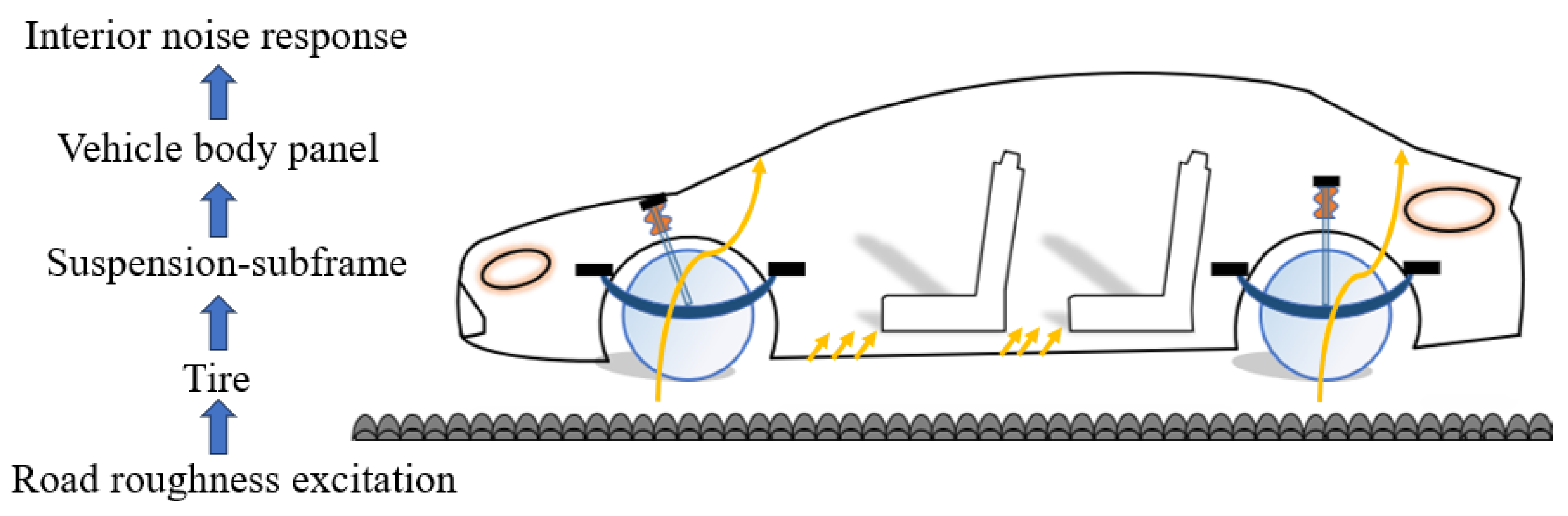
• By analyzing the structure with large noise contribution in the road noise transmission path, the structure with significant influence is defined, the components and quantitative indicators of each level are determined, and the road noise decomposition framework is established.

The structure of the article: Section 2 introduces the relevant theoretical knowledge of LSTM and AFW-LSTM. Section 3 establishes the decomposition framework of road noise based on the analysis of the main influence citation of road noise. Test and collect data according to the decomposition architecture; the CutMix method is used to enhance the sample data obtained from the test to prepare for the model prediction. According to the road noise decomposition architecture, Section 4 uses LSTM, CNN-LSTM, AFW-CNN and AFW-LSTM methods to establish road noise prediction models; the comparison between the predicted value and the real value of the model proves that the AFW-LSTM model is better. The effect of AFW-LSTM model was verified by validation set data. Section 5 summarizes the content of the paper based on the research.

2. Research Methods

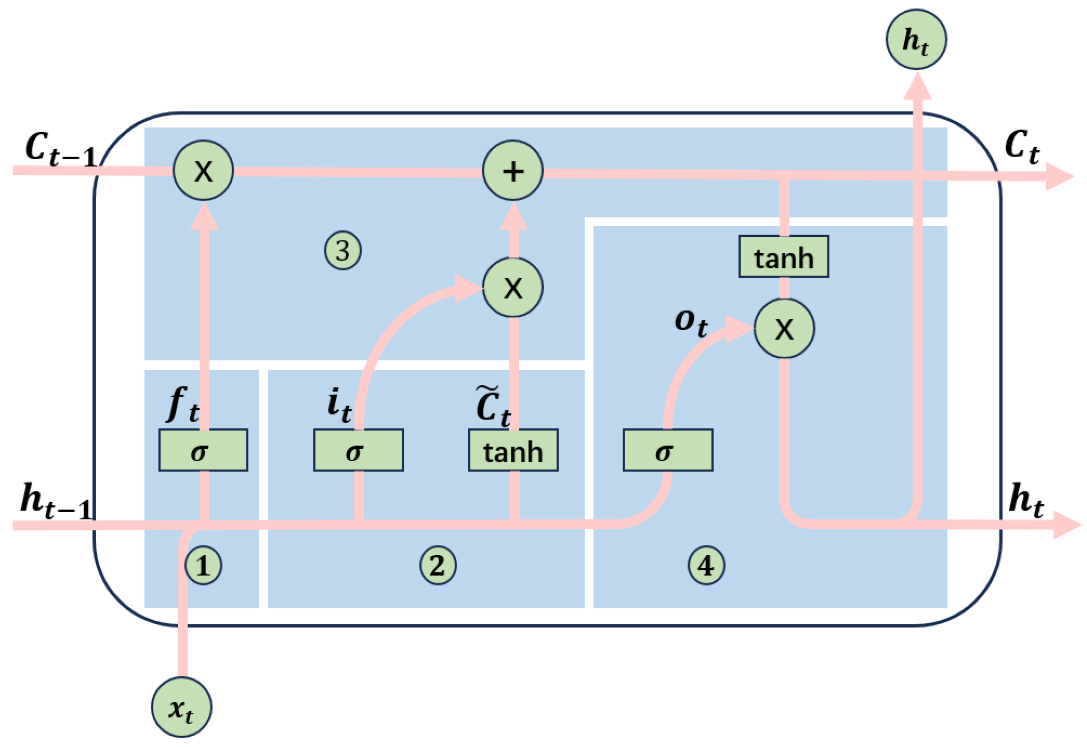
2.1. LSTM Neural Network

As an excellent variant of RNN (Recurrent Neural Network) [26,27], LSTM (Long Short-Term Memory) effectively transmits and expresses useful information in long time series through unique gate mechanism and memory cells, and solves the problem of gradient disappearance and gradient explosion of original RNN [28]. The LSTM is composed of a gating unit. The gating unit judges the input data, leaves the data that conform to the rules, and forgets the data that do not conform to the rules. Its internal structure is shown in Figure 1.

The forgetting gate $f_t$, the input gate $i_t$, the output gate $o_t$ and the memory cell ${\tilde{C}}_t$ of LSTM are shown as follows (1)–(4):

$$f_t=\sigma (W_f[h_{t-1},x_t]+b_f)$$

(1)

$$o_t=\sigma (W_o[h_{t-1},x_t]+b_o)$$

(2)

$$i_t=\sigma (W_i[h_{t-1},x_t]+b_i)$$

(3)

$${\tilde{C}}_t=\tanh (W_{\tilde{C}}[h_{t-1},x_t]+b_{\tilde{C}})$$

(4)

The state of the memory cell is updated by Equation (5), and the output is $C_t$. The calculation of the hidden state is as shown in Equation (6):

$$C_t=f_t\odot C_{t-1}+i_t\odot {\tilde{C}}_t$$

(5)

$$h_t=o_t\odot \tanh (C_t)$$

(6)

where $W_f$, $W_i$ and $W_o$ are the weight matrices of the forgetting gate, the input gate and the output gate, respectively. $b_f$, $b_i$ and $b_o$ are the bias terms of the forgetting gate, input gate and output gate, respectively. $x_t$, $h_t$ and $C_t$ correspond to the current input data, the current output data and the current unit state, respectively. $h_{t-1}$ and $C_{t-1}$ represent the output data and unit state of the previous moment, respectively. ⊙ represents point multiplication, and $\sigma$ represents sigmoid activation function.

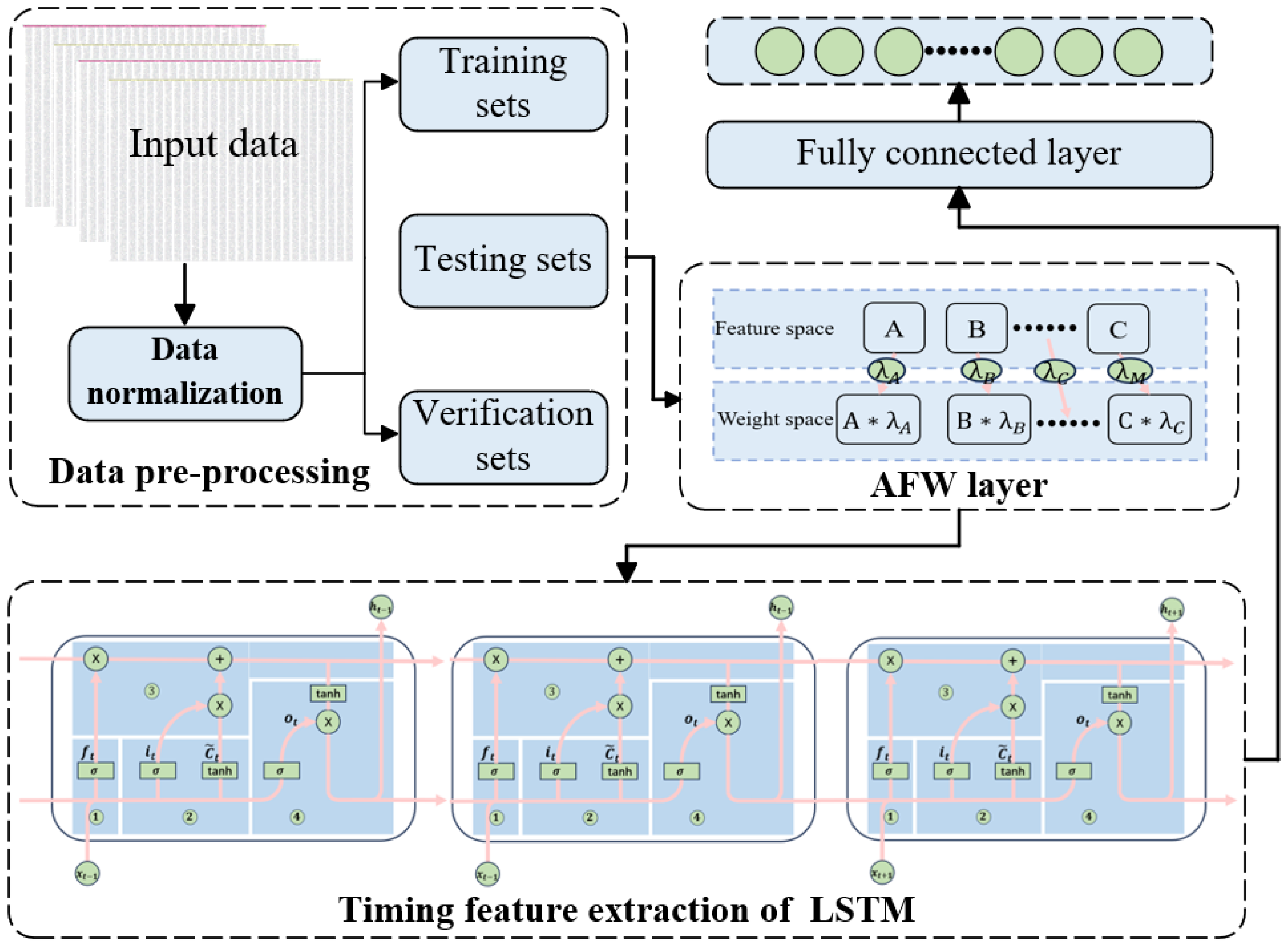
2.2. AFW-LSTM Proposed

Adaptive feature weight (AFW) is inspired by the attention mechanism of the transformer network [29]. The attention mechanism aims to automatically learn and selectively focus on important parts of the sequence during the training process of the neural network, thereby effectively improving the model’s ability to process sequence data and enhancing the performance and generalization of the model. Similarly, adaptive feature weights mimic the attention mechanism to a certain extent and are used to balance the importance of different features or different tasks [30]. The main purpose of adaptive feature weight is to highlight important features by learning a weight distribution. This layer can be used to emphasize or weaken some features of input data in deep learning applications [31] and enhance the model’s ability to understand and process data. In practice, the application of this layer not only helps to improve the performance of the model on specific tasks but also helps to save computing costs. In this paper, when the model is built, an AFW layer is added to apply different weights to the input data column. The processed data are then imported into the neural network for learning, thereby improving the model’s utilization efficiency of useful features. The AFW-LSTM model structure is shown in Figure 2.

The AFW mechanism dynamically assigns weights to each input feature, so the model can adaptively adjust the importance of different features according to the up and down steps of the time series; that is, the input feature is weighted by attention. Suppose $X_t$ is an input feature, as shown in Equation (7):

$$X_{\mathrm{t}}=[x_t^1,x_t^2,\dots ,x_t^n]$$

(7)

where $x_{\mathrm{t}}^i$ represents the ith feature of the tth time step.

The calculation formula of feature weight is shown in Equation (8):

$$w_{\mathrm{t}}^i=\sigma (W_w\cdot x_t^i+b_w)$$

(8)

where $W_w$ is the weight matrix, $b_w$ is the bias term, and $\sigma$ is the Sigmoid activation function.

$$x_t^{weighted}=[w_t^1\cdot x_t^1,w_t^2\cdot x_t^2,\dots ,w_t^n\cdot x_t^n]$$

(9)

The feature weighting layer $x_t^{weighted}$ weights the input features of each time step, and its calculation equation is shown in Equation (9). The weighted input feature $x_t^{weighted}$ is used as the input of LSTM, which improves the learning performance of LSTM network on the basis of better emphasizing or weakening the characteristics of input data.

3. Data Collection and Processing

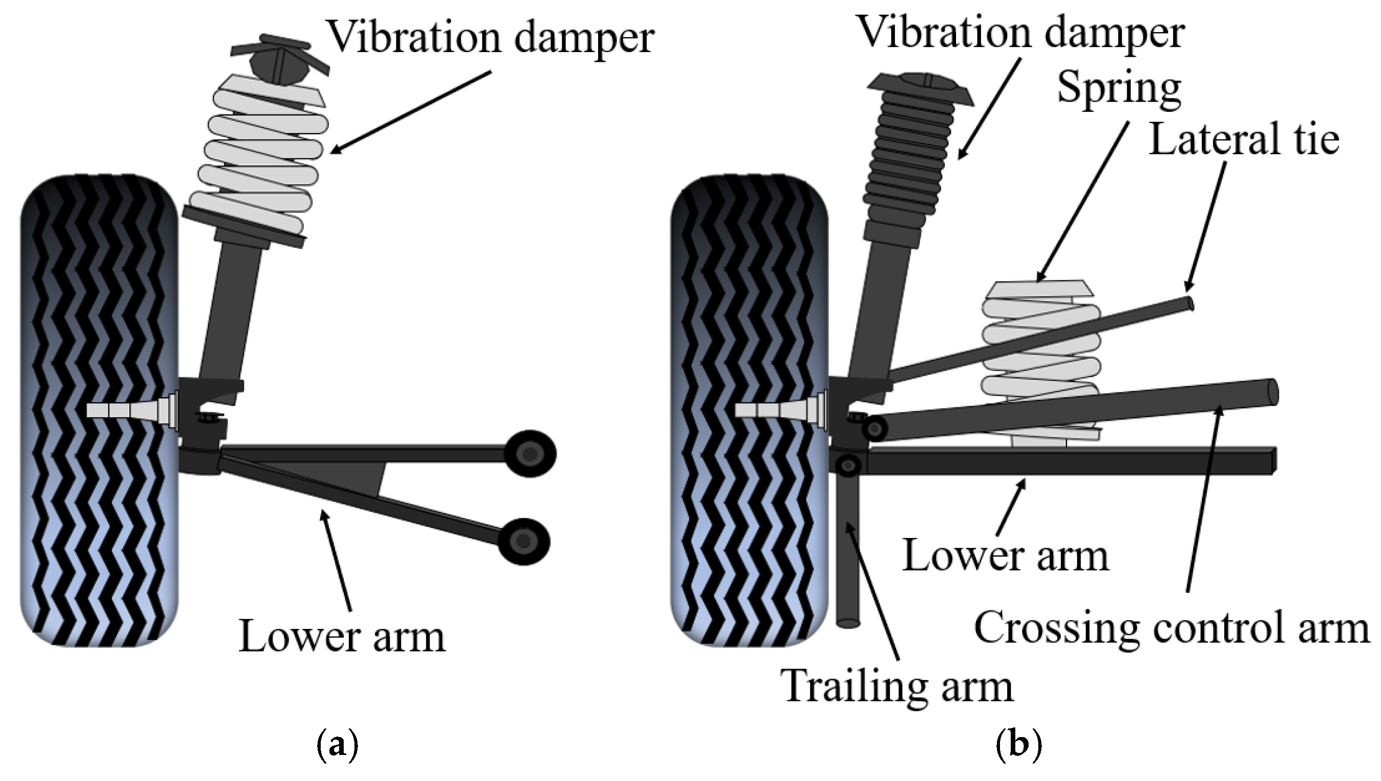
3.1. Analysis of Key Influencing Factors of Road Noise

In this paper, a car with ‘front McPherson and rear multi-link’ suspension is taken as the research object. Road noise is mainly generated by a rolling vehicle tire on the road pavement, including air-borne noise and structural-borne noise [32]. This paper mainly analyzes the road noise of structural transmission noise. The structural transmission noise mainly comes from two aspects: on the one hand, the vertical force generated by the continuous local compression and release of the tire through the contact surface of the road surface, and on the other hand, the longitudinal excitation force generated by the continuous rolling and release of road surface and tire rubber [33,34]. The schematic diagram of road noise formation is shown in Figure 3. When the car is driving on an uneven road surface, the roughness of the road surface will exert force on the tire, and the tire will vibrate. The coupling system of the cavity structure inside the tire and the hub will produce resonance reaction. The vibration is transmitted from the tire and the hub to the suspension, and the suspension transmits the vibration to the subframe, which is then transmitted to the body panel by the subframe. As a larger surface, the body panel will be excited by the vibration and begin to resonate. The sound wave generated by the vibration radiates to the vehicle through the body, thus forming the interior noise of the vehicle. Each link in the transmission process may affect the final road noise performance, so it is necessary to study the related components and propagation paths involved.

The front McPherson and rear multi-link suspension structure is shown in Figure 4. The front McPherson independent suspension [35] is mainly composed of an A-shaped lower swing arm and a shock absorber. The combination of the shock absorber of the McPherson suspension and the helical spring has the advantages of simple structure, small space occupation, good handling performance and low manufacturing cost. The rear multi-link suspension [36] is mainly composed of the lower swing arm, the lateral pull rod, the lateral control arm, the shock absorber, the rear longitudinal arm and the spring. Because the rear multi-link suspension can achieve the best position of the kingpin caster angle, it has straight-line driving stability, acceleration and braking smoothness and comfort. The ‘front McPherson, rear multi-link’ [37] suspension structure can provide better maneuverability and improve the comfort of rear passengers. It is the main suspension structure for consumers who pursue comfort or high-end models.

Without considering the non-main transmission path of road noise such as steering rod and balance rod and the spiral spring with small noise contribution, the road noise transmission path of ‘front McPherson, rear multi-link’ is shown in Figure 5. The excitation obtained by the front and rear knuckles is directly transmitted to the body through the suspension or to the front and rear subframes through the suspension, and then to the body through the front and rear subframes. The unilateral front McPherson suspension has three transfer paths (the A-shaped lower swing arm has two bushings, which are divided into the front mounting point and the rear mounting point), including the steering knuckle–the front mounting point of the front lower swing arm–the front subframe–body, the steering knuckle–the rear mounting point of the front lower swing arm–the front subframe-body, and the steering knuckle–the front shock absorber–body. The single-sided rear multi-link suspension has five transmission paths, including steering knuckle–rear shock absorber–body, steering knuckle–rear longitudinal arm-body, steering knuckle–rear control arm–rear subframe–body, steering knuckle–rear lateral tie rod–rear subframe–body, and steering knuckle–rear lower swing arm–rear subframe–body.

Shock absorber and bushing, as the main damping and vibration isolation components in the suspension system, have a significant impact on road noise. The dynamic parameters of the bushing connector and the vibration acceleration of the active end are the main influencing factors of road noise. Combined with Figure 5, a comprehensive analysis is carried out. Taking the left side as an example, the influencing factors and transmission paths of road noise are analyzed [38]. The vehicle target is decomposed from top–down to the underlying design target layer by layer, and the bottom–up prediction is carried out layer by layer to form the vehicle road noise decomposition architecture, as shown in Figure 6.

The dynamic parameters such as the vibration acceleration excitation of the active end of the lower level, the dynamic stiffness of the bushing, and the damping characteristics of the shock absorber are used as input parameters to predict the noise target of the driver’s right ear of the upper level. The multi-level decomposition framework of road noise includes the following: the first level is the driver’s right ear noise; the second level is the suspension equivalent bushing dynamic stiffness, shock absorber damping and steering knuckle vibration acceleration. The suspension includes the front lower swing arm, the rear lateral tie rod, the rear lateral control arm and the rear longitudinal arm. The shock absorber includes the front and rear shock absorbers, and the steering knuckle includes the front and rear steering knuckles.

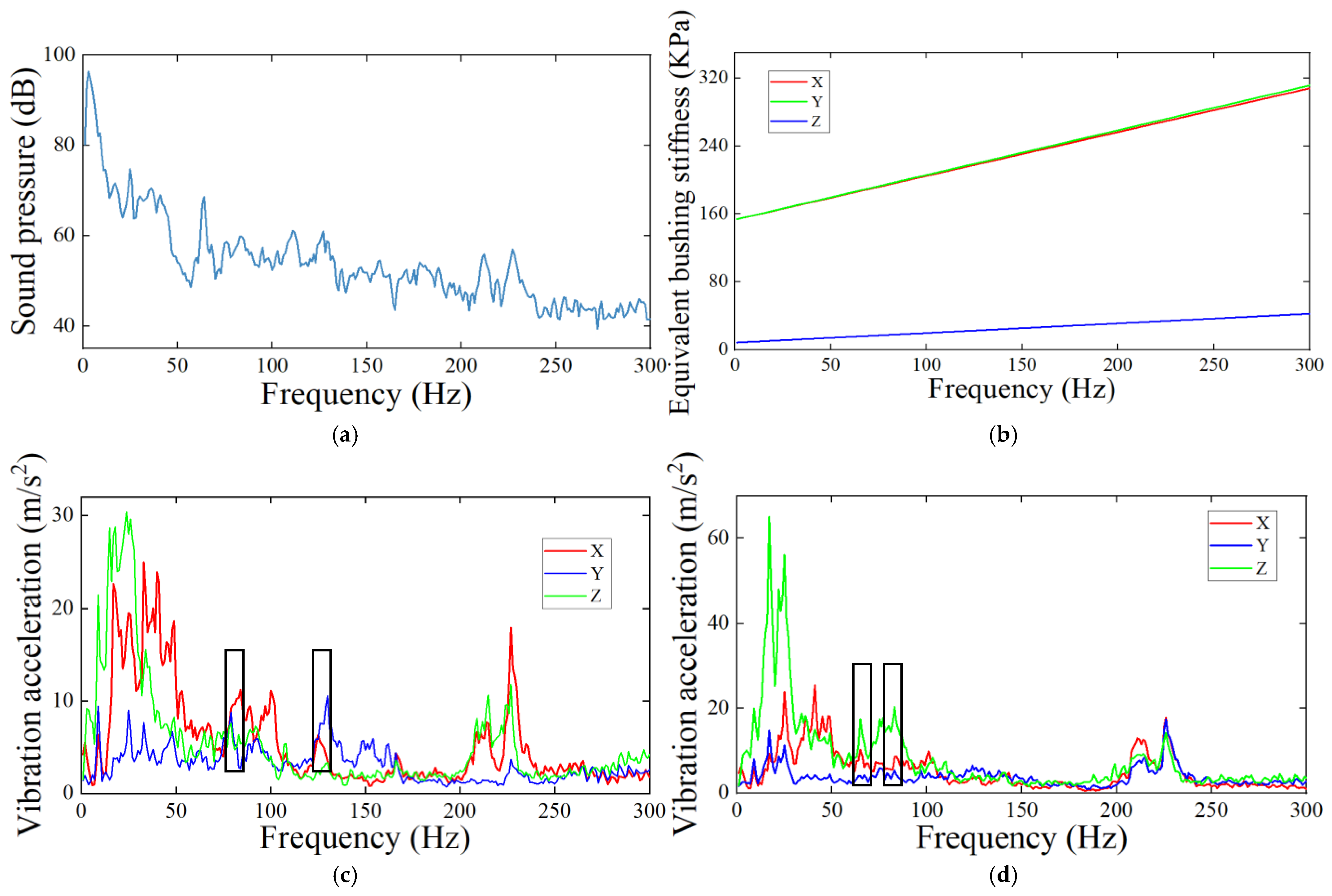
3.2. Data Collection

The noise and vibration data are collected synchronously through the real vehicle road test. The asphalt pavement with rough surface and no three-dimensional buildings and other large objects within 20 m on both sides is selected as the test road. According to the GB/T 18697-2002 [39] automobile interior noise measurement method, a BSWA sound pressure sensor is arranged on the driver’s right ear. The vertical coordinate is (0.70 ± 0.05) m above the intersection of the seat surface and the backrest surface, and the horizontal coordinate is (0.20 ± 0.02) m away from the right side of the seat center surface. In addition, the PCB three-way acceleration sensor is arranged according to the corresponding position of the vibration acceleration in the road noise hierarchical decomposition structure, which is used to collect the vibration acceleration of the steering knuckle. A total of four three-way acceleration sensors are arranged at the steering knuckle of the front, back, left and right tires, plus an ear-side sound pressure sensor. A total of five sensors are arranged in the test. Figure 7 is the position of the left sensor.

The Signature Testing-Advanced module in LMS Test.lab 18 is used to collect data online and analyze and process the data. The schematic diagram of the test process is shown in Figure 8. The road roughness excitation causes noise and vibration in the vehicle. The sensor system tests the noise and vibration acceleration and transmits it to the LMS data acquisition instrument. Finally, it is transmitted to the computer PC through the network, and the data are analyzed and processed by Simcenter Test.lab 18 software.

By modifying the damping and dynamic stiffness parameters of structural components such as shock absorbers and suspensions of vehicles, 16 test prototypes of the same model but different structures are formed. Based on the above vehicles, real vehicle road noise tests were carried out, and a total of 16 sets of test sample data were collected. Due to the large number of sample data obtained from the test, only the data of the noise of the driver’s right ear at the left front installation point of sample 1 are displayed. This part of the data includes the noise of the driver’s right ear, the dynamic stiffness of the equivalent bushing of the left front lower swing arm and the front installation point of the steering knuckle (the same as the bushing of the left front lower swing arm and the rear installation point of the steering knuckle), the vibration acceleration of the left front steering knuckle and the vibration acceleration of the left rear steering knuckle. Considering the actual noise environment characteristics in the vehicle, the frequency band of the test is mainly concentrated between 20 Hz and 300 Hz, as shown in Figure 9a–d; observing the frequency band of 50~150 Hz, we can see that there are resonance peaks at 75 Hz and 130 Hz in Figure 9c, and there are resonance peaks at 55 Hz and 85 Hz in Figure 9d.

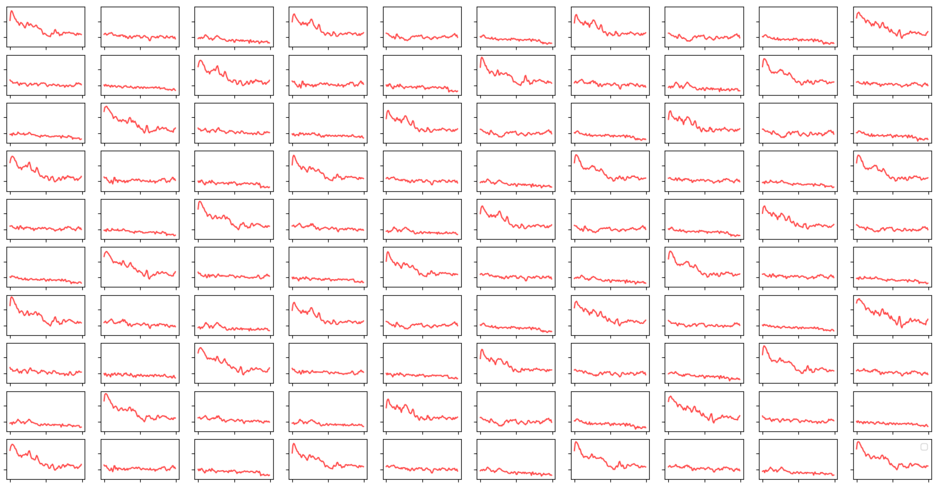
3.3. Data Augmentation

CutMix [40] is different from the Mixup method [41,42], which interpolates two sets of data to form a new sample. It was originally a data enhancement method used in the field of image recognition. By integrating the features of the two sets of data, the model is easier to distinguish them from each other. The data set enhanced by this method has diversity and generalization. The CutMix method used in array data belongs to the mixed data enhancement method [43,44]. It randomly selects some data from multiple arrays to mix and generate a new array to achieve the effect of data enhancement. This method is suitable for sample data with the same dimension. It is assumed that there are two arrays A and B, and the corresponding labels are $y_A$ and $y_B$, respectively. According to Expressions (10) and (11), a new array ($\tilde{A}$, $\tilde{y}$) can be generated:

$$\tilde{A}=\lambda A+(1-\lambda )B$$

(10)

$$\tilde{\mathrm{y}}=\lambda y_A+(1-\lambda )y_B$$

(11)

where $\lambda$ $\in$ [0, 1], and obeys Beta ($\alpha ,\alpha$) distribution, $\alpha$ = 1.0 in this paper.

The enhanced samples generated by the CutMix method are shown in Figure 10, where Figure 10a,b is the sample data when $\lambda$ is 0.1 and 0.9, respectively. It can be seen from the figure that the sample data generated by CutMix is the first half of the original sample 1 plus the new fragment of the second half (the original sample 1 and the original sample 2 are generated according to the value). When $\lambda$ is 0.1, the new fragment data are closer to the original data 2, and when $\lambda$ is 0.9, the new fragment data are closer to the original data 1. Therefore, the larger the value of $\lambda$ is, the closer the enhanced sample generated by the CutMix method is to the data of the original sample 1, and the smaller the value of $\lambda$ is, the closer the enhanced sample generated by the CutMix method is to the data of the original sample 2. In order to make the data generated by the data augmentation have a greater feature difference than the original sample curve and to more fully cover the diversity of the original data set, this paper selects the $\lambda$ value of 0.5. This value can achieve a better balance between the original curve 1 and the original curve 2, thereby improving the diversity of the data set and the generalization ability of the model.

Since the 16 sets of original sample data collected by the experimental method face difficulty in meeting the needs of model training, the CutMix method is introduced to expand the original data samples, and finally, 102 sets of sample data are obtained. For typesetting considerations, only 100 sets of samples are displayed. At the same time, considering that there are many factors affecting road noise and that the transmission path is complex, only the extended data schematic diagram of the first-level driver’s right ear noise data is displayed, as shown in Figure 11.

4. Road Noise Prediction Model

4.1. Construction of AFW-LSTM Road Noise Model

Due to the large numerical span between the input variable and the output variable, in order to improve the training accuracy of the model, it is necessary to normalize the data before entering the model, so that the scale is consistent when the data are imported [45]. After the 102 sets of sample data are normalized to the [0, 1] interval, in order to train and evaluate the prediction performance of the model, the data need to be divided into training set, test set and verification set. In this paper, the training set and the test set are divided according to 8:2; that is, 80 groups of model training are used to fine-tune and determine the model parameters, and 20 groups of model tests were carried out to test the rationality of model parameter setting. Two groups of model validation were used to evaluate the results of the hierarchical prediction model, that is, the difference between the predicted value of the model and the true value. The data-driven algorithm is introduced to fit the data mapping relationship between entities at all levels through the big data learning characteristics of the neural network, so as to realize the construction and prediction of the road noise prediction model. The construction process is shown in Figure 12.

According to the flow chart of the prediction model, LSTM, CNN-LSTM (Convolutional Neural Networks-Long Short-Term Memory), AFW-CNN (Adaptive feature weight-Long Short-Term Memory) and AFW-LSTM prediction models are built. Taking the AFW-LSTM model as an example, the structure of the prediction model is shown in Figure 13. Taking the driver’s right ear noise as an example, the input layer size of the AFW-LSTM and LSTM networks is 48, the hidden layer size is 64, the output layer size is 1, the optimizer is Adam, and the learning rate is 0.001. The input channel size of AFW-CNN networks is 48, the output channel is 12, the kernel size is 2, the step size is 1, the optimizer is SGD (stochastic gradient descent), the learning rate is 0.001, and the momentum is 0.9. The dropout is set to 0.4, the epoch is set to 300, and the batch size is set to 4 in the hidden layer of LSTM, CNN-LSTM, AFW-CNN and AFW-LSTM models. The AFW-LSTM model is built based on Figure 13. At the same time, the sample data set collected by the test and enhanced by the CutMix method is imported into the model, and the prediction is carried out according to the road noise decomposition architecture. Finally, the prediction results of the driver’s right ear noise are obtained. The data are randomly disrupted before being imported into the prediction model. Since no fixed random seeds are set, the order of data disruption during each training will be different, and different training sets and test sets will be obtained each time.

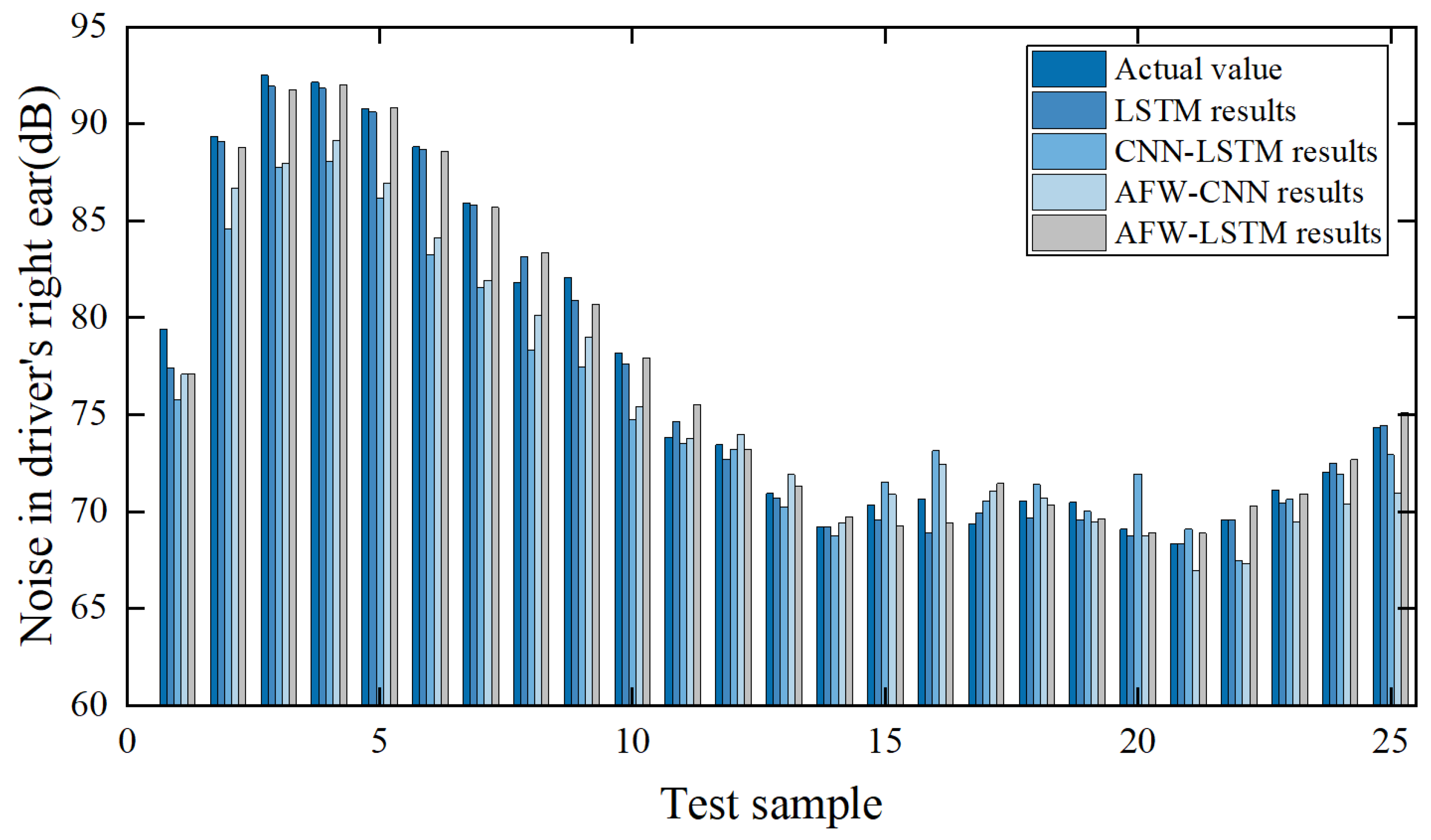
4.2. AFW-LSTM Road Noise Model Prediction and Results Comparison

In order to compare the results of the four neural network models, the driver’s right ear noise prediction results with an output of 300 $\times$ 1 are shown in Figure 14, including the driver’s right ear noise prediction results comparison chart: (a) LSTM prediction results, (b) CNN-LSTM prediction results, (c) AFW-CNN prediction results, and (d) AFW-LSTM prediction results. It can be clearly concluded that the predicted values of the AFW-LSTM model and the AFW-CNN model are in good agreement with the linear trend of the true values, which proves that the AFW-LSTM model and the AFW-CNN model can effectively predict the driver’s right ear noise. On this basis, the prediction results of the LSTM model in AFW mode are compared with the prediction results of the basic LSTM model, and the prediction results of the CNN model in AFW mode are compared with the prediction results of the AFW-LSTM model. The prediction results of the AFW-LSTM model are not only better than the prediction results of the CNN-LSTM model, but also better than the prediction results of the AFW-CNN model. The AFW-LSTM model has a higher degree of coincidence between the predicted results and the real value trend, and the accuracy of the predicted results is also better.

In order to compare and evaluate the prediction results of different road noise models more objectively, RMSE [46,47] (root mean square error), MAE (mean absolute error) and $R^2$ [48] (coefficient of determination) are selected to quantify the effect of the model. The smaller the RMSE and MAE values are, the closer the predicted value is to the true value, and the higher the prediction accuracy is. $R^2$ is calculated by the real value and the predicted value in the frequency domain according to the corresponding formula, and the value range is [0, 1]. The closer the value is to 1, the better the model fitting effect is, and the closer it is to 0, the effect is the opposite. The expressions of each index are as follows in Equations (12)–(14):

$$RMSE=\sqrt{{\displaystyle \frac{1}{n}}{\displaystyle \sum _{i=1}^n{(y_i-{\widehat{y}}_i)}^2}}$$

(12)

$$MAE={\displaystyle \frac{1}{n}}{\displaystyle \sum _{i=1}^n|y_i-{\widehat{y}}_i|}$$

(13)

$$R^2=1-{\displaystyle \frac{{\displaystyle \sum _{i=1}^n({\mathrm{y}}_i-{\widehat{y}}_i{)}^2}}{{\displaystyle \sum _{i=1}^n{(y_i-{\overline{y}}_i)}^2}}}$$

(14)

where n is the number of samples, $y_i$ is the true value, ${\widehat{y}}_i$ is the predicted value, and ${\overline{y}}_i$ is the mean value of the true value.

As shown in

Table 1. Comparison of driver’s right ear noise results.

Index	LSTM	CNN-LSTM	AFW-CNN	AFW-LSTM
RMSE (dB)	1.91	1.90	1.76	1.74
MAE (dB)	2.69	2.72	2.61	2.60
$R^2$	0.901	0.890	0.913	0.924

, the prediction results of the LSTM model, CNN-LSTM model, AFW-CNN model and AFW-LSTM model are analyzed and compared. The root mean square error of the AFW-LSTM model is 1.74 (dB), which is lower than 1.91 (dB) of the LSTM model, 1.90 (dB) of the CNN-LSTM model and 1.76 (dB) of the AFW-CNN model. The average absolute error of the AFW-LSTM model is 2.6 (dB), which is lower than 2.69 (dB) of the LSTM model, 2.72 (dB) of the CNN-LSTM model and 2.61 (dB) of the AFW-CNN model. At the same time, the determination coefficient of AFW-LSTM is the closest to 1, which proves that the model has high prediction accuracy and good fitting effect.

4.3. Verification of Prediction Results of AFW-LSTM Road Noise Model

The sample data that did not participate in model training and model testing were selected as the validation set, and the prediction effect of the trained road noise prediction model was verified by the validation set [49,50]. The validation set plays a key role in ensuring the generalization ability of the model and the effectiveness of practical applications. Figure 15 only shows the histogram comparison results of the first 25 sampling points. From the graph, it can be seen that compared with the other three prediction models, the AFW-LSTM model has higher prediction accuracy and better generalization.

According to the above diagram, it can be seen that the AFW-LSTM prediction model established in this paper has a significant effect. The true value of the verification set is highly coincident with the trend of the predicted value of the model. In order to show the difference in each prediction model more intuitively, the results of the unified index are shown in

Table 2. Comparison of driver’s right ear noise results (validation set).

Index	LSTM	CNN-LSTM	AFW-CNN	AFW-LSTM
RMSE (dB)	1.85	1.94	2.00	1.84
MAE (dB)	2.67	2.73	2.77	2.66
$R^2$	0.891	0.871	0.908	0.912

. The root means square errors of the prediction results of the LSTM model, CNN-LSTM model, AFW-CNN model and AFW-LSTM model are 1.85 (dB), 1.94 (dB), 2.00 (dB) and 1.84 (dB), respectively. The average absolute errors are 2.67 (dB), 2.73 (dB), 2.77 (dB) and 2.66 (dB), respectively. The coefficients of determination are 0.891, 0.871, 0.908 and 0.912, respectively. The AFW-LSTM model based on the validation set data is superior to the other three prediction models. In addition, the performance of the model on the validation set is consistent with that on the test set, and the overall performance prediction error of the model is not higher than $\pm$2 dB, indicating that the model has good generalization ability and robustness.

5. Conclusions

• Based on the theory of road noise transfer path, the factors and paths that have significant influence on road noise such as steering knuckle, suspension and shock absorber are analyzed, and a two-level decomposition framework of road noise with key influencing factors as input and driver’s right ear noise as output is established. Based on the hierarchical structure of road noise, the road test is carried out, and 16 sets of complete road noise sample data are collected. The data set is enhanced by the CutMix method, where $\lambda$ = 0.5, $\alpha$ = 1.0, and 102 sets of sample data are generated.
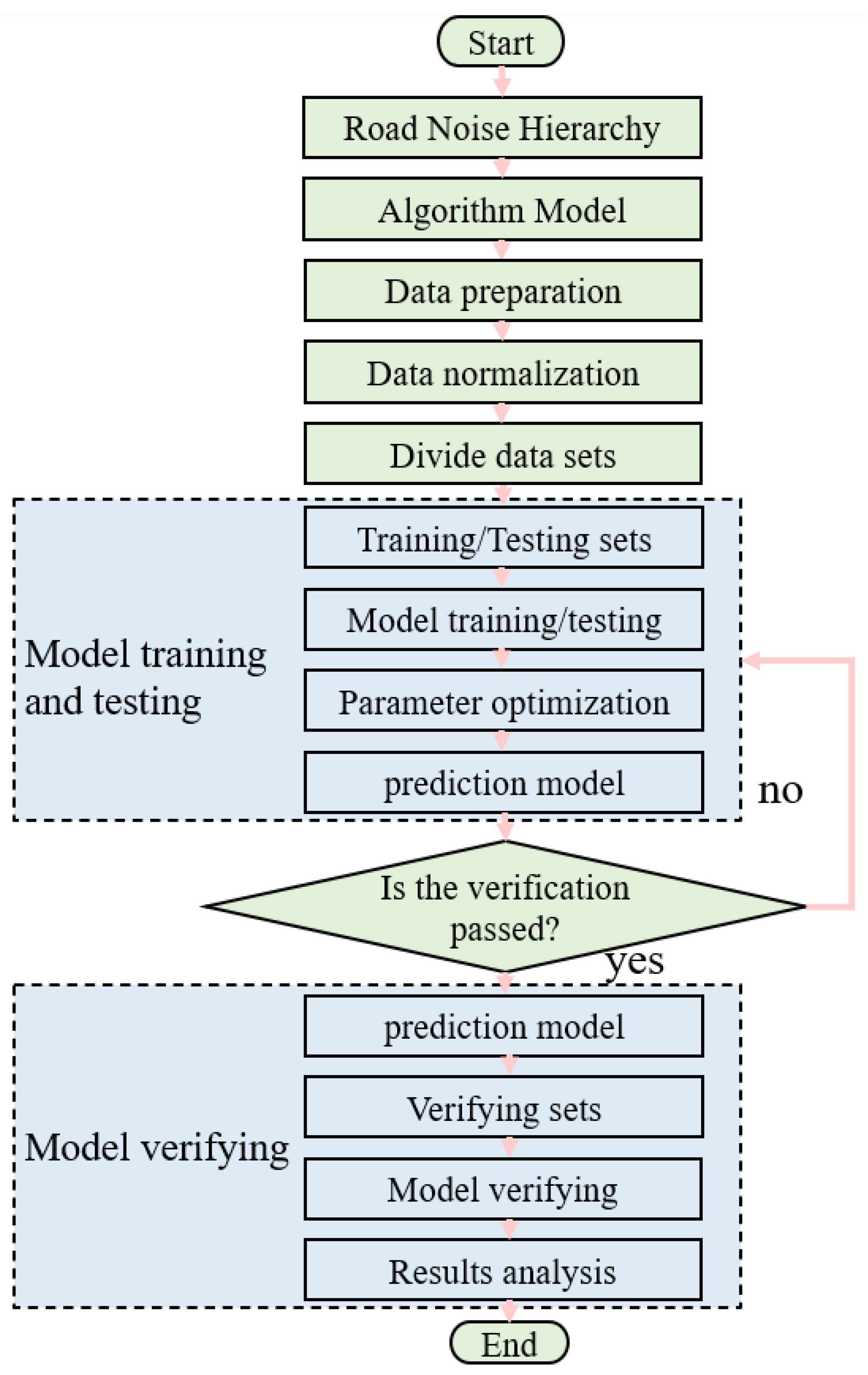
• Based on the road noise hierarchical decomposition architecture, a data-driven model is built for the proposed AFW-LSTM method to reveal the quantitative relationship of the associated units in the hierarchical system. Data preprocessing involves data normalization, data set division, etc. The model training obtains the implicit mapping relationship between the levels of data and can obtain the data law of the frequency point analysis. At the same time, the prediction results of the data-driven model built by the four methods of LSTM, CNN-LSTM, AFW-CNN and AFW-LSTM are compared. The analysis results show that RMSE = 1.74 (dB), MAE = 2.6 (dB), $R^2$ = 0.924. Under the background of road noise, the prediction result of LSTM model is better than that of CNN prediction model, and the accuracy of LSTM model with AFW layer is better than that of single neural network model.
• The proposed method is tested by the sample data of the verification set obtained from the specific vehicle model. The results show that the predicted value is in good agreement with the true value, and the accuracy and robustness of the AFW-LSTM prediction model show obvious advantages. The RMSE = 1.84 (dB), MAE = 2.66 (dB), $R^2$ = 0.912 and other indicators obtained by the AFW-LSTM model are better than the models built by LSTM, CNN-LSTM, and AFW-CNN methods. Adaptive feature weight is conducive to the model to learn more important content, which can improve the efficiency and accuracy of the model to process data.
• The road noise prediction model only analyzes the influence of the suspension part on the driver’s right ear noise. The body part is still an important factor affecting the interior noise. In future research, the body parameters will be introduced to analyze the road noise problem. In addition, although the adaptive weight layer can enhance the network’s emphasis on key features under the premise of controllable actual engineering data and training, its comparative study with the current mainstream attention mechanism still needs to be further improved and expanded in the future.

References

1. Huang, H.; Huang, X.; Ding, W.; Yang, M.; Yu, X.; Pang, J. Vehicle vibro-acoustical comfort optimization using a multi-objective interval analysis method. Expert Syst. Appl. 2023, 213, 119001. [Google Scholar] [CrossRef]
2. Huang, H.; Wang, Y.; Wu, J.; Ding, W.; Pang, J. Prediction and optimization of pure electric vehicle tire/road structure-borne noise based on knowledge graph and multi-task ResNet. Expert Syst. Appl. 2024, 255, 124536. [Google Scholar] [CrossRef]
3. Wang, H.; Liang, H.; Yu, D.; Hou, Q.; Zeng, W. A new urban road traffic noise exposure assessment method based on building land-use types and temporal traffic demand estimation. J. Environ. Manag. 2025, 376, 124604. [Google Scholar] [CrossRef] [PubMed]
4. Petri, D.; Licitra, G.; Vigotti, M.A.; Fredianelli, L. Effects of Exposure to Road, Railway, Airport and Recreational Noise on Blood Pressure and Hypertension. Int. J. Env. Res. Public Health 2021, 18, 9145. [Google Scholar] [CrossRef]
5. Fu, J.; Zhu, C.; Su, J. Research on the Design Method of Pure Electric Vehicle Acceleration Motion Sense Sound Simulation System. Appl. Sci. 2023, 13, 147. [Google Scholar] [CrossRef]
6. Thakur, A.; Krishnan, K.; Ansari, A. Powering the transition: Examining factors influencing the intention to adopt electric vehicles. Smart Sustain. Built Environ. 2025, 14, 471–488. [Google Scholar] [CrossRef]
7. Zhao, J.; Yin, Y.; Chen, J.; Zhao, W.; Ding, W. Evaluation and prediction of vibration comfort in engineering machinery cabs using random forest with genetic algorithm. SAE Int. J. Veh. Dyn. Stab. NVH 2024, 8, 491–512. [Google Scholar] [CrossRef]
8. Jadhav, P.; Waghulde, K.; Bhortake, R. Test and CAE vibration results correlation and isolator design for improvement of car door vibrations. Int. J. Interact. Des. Manuf. 2024, 1–14. [Google Scholar] [CrossRef]
9. Park, U.; Kang, Y. Operational transfer path analysis based on neural network. J. Sound Vib. 2024, 579, 118364. [Google Scholar] [CrossRef]
10. Cao, Y.; Wang, D.; Zhao, T. Electric vehicle interior noise contribution analysis. SAE Tech. Pap. 2016, 7. [Google Scholar] [CrossRef]
11. Vaitkus, D.; Tcherniak, D.; Brunskog, J. Application of vibro-acoustic operational transfer path analysis. Appl. Acoust. 2019, 154, 201–212. [Google Scholar] [CrossRef]
12. Zhu, Y.; Lu, C.; Liu, Z.; Song, W.; Xie, L.; Shen, J. Simulated Operational Path Analysis Method for the Separation of Intake and Exhaust Noises. Acoust. Aust. 2020, 48, 261–270. [Google Scholar] [CrossRef]
13. Zhu, H.; Zhao, J.; Wang, Y.; Ding, W.; Pang, J.; Huang, H. Improving of pure electric vehicle sound and vibration comfort using a multi-task learning with task-dependent weighting method. Measurement 2024, 233, 114752. [Google Scholar] [CrossRef]
14. Asdrubali, F.; D’Alessandro, F. Innovative Approaches for Noise Management in Smart Cities: A Review. Curr. Pollut. Rep. 2018, 4, 143–153. [Google Scholar] [CrossRef]
15. Fredianelli, L.; Carpita, S.; Bernardini, M.; Del Pizzo, L.; Brocchi, F.; Licitra, G. Traffic Flow Detection Using Camera Images and Machine Learning Methods in ITS for Noise Map and Action Plan Optimization. Sensors 2022, 22, 1929. [Google Scholar] [CrossRef]
16. Su, J.; Lou, J.; Jiang, X. Research on optimization control of vehicle road noise performance. IOP Conf. Ser. Earth Environ. Sci. 2021, 769, 042055. [Google Scholar] [CrossRef]
17. Gerwin, P.; Georg, J.; Joerg, B. Numerical Transfer Path Analysis for NVH System-Simulation Models. IOP Conf. Ser. Mater. Sci. Eng. 2021, 1097, 012008. [Google Scholar] [CrossRef]
18. Cao, C.; Meng, D.; Zhao, Y.; Shu, Y.; Zhang, M.; Zhang, L. Prediction and Optimization of Full-Vehicle Road Noise Based on Random Response Analysis. J. Phys. Conf. Ser. 2021, 1828, 012166. [Google Scholar] [CrossRef]
19. Yu, W. Analysis and Optimization of Low-Speed Road Noise in Electric Vehicles. Wirel. Commun. Mob. Comput. 2021, 2021, 5537704. [Google Scholar] [CrossRef]
20. Shang, Z.; Hu, F.; Zeng, F.; Wei, L.; Xu, Q.; Wang, J. Research of transfer path analysis based on contribution factor of sound quality. Appl. Acoust. 2021, 173, 107693. [Google Scholar] [CrossRef]
21. Li, M.; Zhou, W.; Liu, J.; Zhang, X.; Pan, F.; Yang, H.; Luo, D. Vehicle interior noise prediction based on Elman neural network. Appl. Sci. 2021, 11, 8029. [Google Scholar] [CrossRef]
22. Pang, J.; Mao, T.; Jia, W.; Jia, X.; Dai, P.; Huang, H. Prediction and Analysis of Vehicle Interior Road Noise Based on Mechanism and Data Series Modeling. Sound Vib. 2024, 58, 59–80. [Google Scholar] [CrossRef]
23. Huang, X.; Huang, H.; Wu, J.; Yang, M.; Ding, W. Sound quality prediction and improving of vehicle interior noise based on deep convolutional neural networks. Expert Syst. Appl. 2020, 160, 113657. [Google Scholar] [CrossRef]
24. Wang, X.; Lin, J.; Liang, H.; Wang, H. A regional road network traffic noise limit prediction method based on design elements. J. Acoust. Soc. Am. 2025, 157, 527–537. [Google Scholar] [CrossRef]
25. Wang, H.; Wu, Z.; Wu, Z.; Hou, Q. Urban network noise control based on road grade optimization considering comprehensive traffic environment benefit. J. Environ. Manag. 2024, 364, 121451. [Google Scholar] [CrossRef]
26. Li, D.; Li, M.; Han, G.; Li, T. A combined deep learning method for internet car evaluation. Neural Comput. Appl. 2021, 33, 4623–4637. [Google Scholar] [CrossRef]
27. Liao, Y.; Qian, F.; Zhang, R.; Kumar, P. Long short-term memory (LSTM) neural networks for predicting dynamic responses and application in piezoelectric energy harvesting. Smart Mater. Struct. 2024, 33, 075005. [Google Scholar] [CrossRef]
28. Noh, S. Analysis of Gradient Vanishing of RNNs and Performance Comparison. Information 2021, 12, 442. [Google Scholar] [CrossRef]
29. Guo, H.; Chen, L.; Wang, Z.; Lin, L. Day-ahead prediction of electric vehicle charging demand based on quadratic decomposition and dual attention mechanisms. Appl. Energy 2025, 381, 125198. [Google Scholar] [CrossRef]
30. Li, T.; Ren, H.; Li, C. Intelligent electric vehicle trajectory tracking control algorithm based on weight coefficient adaptive optimal control. Trans. Inst. Meas. Control 2024, 46, 2647–2663. [Google Scholar] [CrossRef]
31. Huang, H.; Huang, X.; Ding, W.; Yang, M.; Fan, D.; Pang, J. Uncertainty optimization of pure electric vehicle interior tire/road noise comfort based on data-driven. Mech. Syst. Signal Process. 2022, 165, 108300. [Google Scholar] [CrossRef]
32. Wu, Y.; Liu, X.; Huang, H.; Wu, Y.; Ding, W.; Yang, M. Multi-Objective Prediction and Optimization of Vehicle Acoustic Package Based on ResNet Neural Network. Sound Vib. 2023, 57, 73–95. [Google Scholar] [CrossRef]
33. Yang, M.; Dai, P.; Yin, Y.; Wang, D.; Wang, Y.; Huang, H. Predicting and optimizing pure electric vehicle road noise via a locality-sensitive hashing transformer and interval analysis. ISA Trans. 2024, 157, 556–572. [Google Scholar] [CrossRef] [PubMed]
34. Lu, X.; Chen, H.; He, X. A Frequency Domain Fitting Algorithm Method for Automotive Suspension Structure under Colored Noise. World Electr. Veh. J. 2024, 15, 410. [Google Scholar] [CrossRef]
35. GB/T 18697-2002[S]; National Acoustic Standardization Technical Committee. Interior Noise Measurement Method of Acoustic Vehicle. China Standards Publishing House: Beijing, China, 2002.
36. Dwivedi, V.D.; Wahi, P. Influence of gravity on the vibration characteristics of a geometrically nonlinear McPherson-suspension model. Multibody Syst. Dyn. 2024, 61, 571–596. [Google Scholar] [CrossRef]
37. Alizadeh, R.; Fataliyev, V.; Akhundov, E. Improving the Design of the Linkage Suspension of a Robotic Mobile Modular System. J. Mach. Manuf. Reliab. 2024, 53, 539–543. [Google Scholar] [CrossRef]
38. Fan, D.; Dai, P.; Yang, M.; Jia, W.; Jia, X.; Huang, H. Research on maglev vibration isolation technology for vehicle road noise control. SAE Int. J. Veh. Dyn. Stab. NVH 2022, 6, 233–245. [Google Scholar] [CrossRef]
39. Barnett, J.; Li, W.; Resmerita, E. Multiscale Hierarchical Decomposition Methods for Images Corrupted by Multiplicative Noise. J. Math. Imaging Vis. 2025, 67, 12. [Google Scholar] [CrossRef]
40. Yun, S.; Han, D.; Oh, S.; Chun, S.; Choe, J.; Yoo, Y. Cutmix: Regularization strategy to train strong classifiers with localizable features. In Proceedings of the IEEE/CVF International Conference on Computer Vision, Honolulu, HI, USA, 19–23 October 2019; p. 6023. [Google Scholar] [CrossRef]
41. Zhang, H.; Cissé, M.; Dauphin, Y.; Lopez-Paz, D. Mixup: Beyond empirical risk minimization. arXiv 2017, arXiv:1710.09412. [Google Scholar] [CrossRef]
42. Darkwah, Y.; Kang, D. Enhancing few-shot learning using targeted mixup. Appl. Intell. 2025, 55, 279. [Google Scholar] [CrossRef]
43. Zhang, C.; Xu, Y.; Yang, J.; Li, X. Automatic modulation classification based on Alex Net with data augmentation. J. China Univ. Posts Telecommun. 2022, 29, 51–61. [Google Scholar] [CrossRef]
44. Wang, Z.; Yang, S.; Qin, H.; Liu, Y.; Wang, J. MixCFormer: A CNN–Transformer Hybrid with Mixup Augmentation for Enhanced Finger Vein Attack Detection. Electronics 2025, 14, 362. [Google Scholar] [CrossRef]
45. Liao, Y.; Huang, H.; Chang, G.; Luo, D.; Xu, C.; Wu, Y. Research on low-frequency noise control of automobiles based on acoustic metamaterial. Materials 2022, 15, 3261. [Google Scholar] [CrossRef]
46. Wang, W.; Lu, Y. Analysis of the Mean Absolute Error (MAE) and the Root Mean Square Error (RMSE) in Assessing Rounding Model. IOP Conf. Ser. Mater. Sci. Eng. 2018, 324, 012049. [Google Scholar] [CrossRef]
47. Huang, H.; Wu, J.; Lim, T.C.; Yang, M.; Ding, W. Pure electric vehicle nonstationary interior sound quality prediction based on deep CNNs with an adaptable learning rate tree. Mech. Syst. Signal Process. 2021, 148, 107170. [Google Scholar] [CrossRef]
48. Nakagawa, S.; Schielzeth, H. A general and simple method for obtaining R sup2/sup from generalized linear mixed-effects models. Methods Ecol. Evol. 2013, 4, 133–142. [Google Scholar] [CrossRef]
49. Sun, P.; Dai, R.; Li, H.; Zheng, Z.; Wu, Y.; Huang, H. Multi-Objective Prediction of the Sound Insulation Performance of a Vehicle Body System Using Multiple Kernel Learning–Support Vector Regression. Electronics 2024, 13, 538. [Google Scholar] [CrossRef]
50. Marotta, R.; Strano, S.; Terzo, M.; Tordela, C. Multi-output physically analyzed neural network for the prediction of tire–road interaction forces. SAE Int. J. Veh. Dyn. Stab. NVH 2024, 8, 285–308. [Google Scholar] [CrossRef]
Figure 1. LSTM internal structure diagram.
Machines 13 00425 g001
Figure 2. AFW-LSTM structure schematic diagram.
Machines 13 00425 g002
Figure 3. Road noise formation diagram.
Machines 13 00425 g003
Figure 4. ‘Front McPherson, rear multi-link’ suspension structure diagram: (a) front McPherson suspension; (b) rear multi-link suspension.
Machines 13 00425 g004
Figure 5. ‘Front McPherson, rear multi-link’ road noise transmission path.
Machines 13 00425 g005
Figure 6. Road noise decomposition architecture (left).
Machines 13 00425 g006
Figure 7. Sensor placement (left side).
Machines 13 00425 g007
Figure 8. Test flow diagram.
Machines 13 00425 g008
Figure 9. The partial data schematic diagram of sample 1: (a) the driver’s right ear noise; (b) the front installation point of the front lower swing arm and the dynamic stiffness of the steering knuckle bushing; (c) the vibration acceleration of the left front steering knuckle; (d) the vibration acceleration of the left rear steering knuckle. The black boxes represent the resonance peaks.
Machines 13 00425 g009
Figure 10. CutMix enhances the sample data: (a) the sample enhancement when λ = 0.1; (b) the sample enhancement when λ = 0.9.
Machines 13 00425 g010
Figure 11. DA data faceted diagram.
Machines 13 00425 g011
Figure 12. Flow chart of prediction model.
Machines 13 00425 g012
Figure 13. AFW-LSTM.
Machines 13 00425 g013
Figure 14. Comparison of driver’s right ear noise prediction results: (a) LSTM prediction results; (b) CNN-LSTM prediction results; (c) AFW-CNN prediction results; (d) AFW-LSTM prediction results.
Machines 13 00425 g014
Figure 15. Comparison of prediction results based on validation set data.
Machines 13 00425 g015