Integral Linear Quadratic Regulator Sliding Mode Control for Inverted Pendulum Actuated by Stepper Motor

Abstract

Stabilization and tracking problems for cart inverted pendulums under disturbances and uncertainties have posed significant challenges for control engineers. While various controllers have been designed for an inverted pendulum, they often overlook the calibration error of the pendulum angle in practical implementations, which degrades the control performance. Incorrect calibration of the pendulum angle in upright equilibrium position generates an offset of cart position errors. To solve this problem, an augmented model comprising integral cart position errors was first constructed. Afterwards, a sliding mode control was designed for this system based on a linear quadratic controller, to facilitate implementation. Additionally, a stepper motor was employed in the inverted pendulum to enhance the control performance and widen applicability in industrial settings. The effectiveness and performance of the proposed controller were validated by means of experimental studies, focusing on stabilization control and tracking control of a cart inverted pendulum actuated by a stepper motor.

1. Introduction

Recently, under-actuated mechanical systems (UMSs) have gained increased attention regarding both linear and non-linear control, due to their potential to reduce manufacturing cost, weight, and failure rate, thereby increasing reliability [1]. In such a system, the number of actuators is less than the degree of freedom, and the unactuated degree of freedom may be indirectly controlled by dynamic coupling. One of the most famous classes of UMSs is a cart inverted pendulum (CIP), a simple structure with two degrees of freedom and one control input. The CIP finds its application in real-time scenarios such as rockets and missiles, heavy crane lifting containers, and self-balancing robots [2], emphasizing the importance of control design for CIPs. A typical CIP exhibits a stable equilibrium point at the pending position and an unstable equilibrium point at the upright positions [3]. In the transitions from the pending position to the upright positions, the model becomes strongly non-linear with respect to the pendulum angle [4]. Depending on the control purpose of the CIP, several studies have tried to independently solve the swing-up, stabilization, and tracking problems. However, in practical scenarios, the problems of stabilization and tracking control have gained more attention for real-time applications than the problem of swing-up control [5].

Despite the inherent non-linearity and coupling in a CIP system, typically described by non-linear differential equations, it is common practice to obtain approximate linear models around the operating point to design the control for the stabilization and tracking position in a CIP. Several designs of controller and analysis techniques for linear systems have been proposed for CIPs to address stabilization and tracking problems, such as proportion integral derivative (PID) [6,7,8] and linear quadratic regulator (LQR) [9,10,11]. While a PID controller is designed based on errors, without requiring knowledge of the CIP system, an LQR employs a nominal model of the CIP to determine the control input. The LQR is an important technique in modern optimal control theory for solving the state feedback control problem [12], guaranteeing the stability and phase margins of the control system [13]. An LQR controller is robust against minor external disturbances and can achieve a smaller oscillation amplitude than pole placement control in the stabilization problem of CIPs [10,14]. However, LQR control can cause an offset of cart position in the CIP system, due to disturbances and uncertainties. In response, an integral linear quadratic regulator (ILQR) [15,16] was proposed, aiming to mitigate this offset issue by incorporating the integral action of the cart position into the LQR framework in the CIP system [17]. Nevertheless, the performance of these controllers can be degraded in the presence of major disturbances and uncertainties, since they belong to the linear controller class [18].

To overcome this limitation, the sliding mode control (SMC) developed by Utkin [19] has emerged as one of the most robust controls for ensuring the stability and performance of a CIP under uncertainties and external disturbances. The conventional SMC design methodology comprises two steps: first, designing a sliding manifold to ensure the system’s motion along the manifold meets the specified performance; second, designing a control law to drive the system’s state toward the manifold and maintain it there from then on. There are two main directions in control design for CIPs: hierarchical sliding mode control, and conventional sliding mode control. Using SMC in a hierarchical structure not only retains the advantages of SMC, but also enables simultaneous control of different outputs [20]. This strategy decomposes the system into subsystems, and designs an individual sliding surface for each. The ultimate control law is then formulated based on a composite sliding surface, which integrates the sliding surface of subsystems [21]. By implementing this method, a high-dimensional system is effectively reduced to lower-dimensional subsystems, simplifying the controller design. Linear hierarchical sliding mode control (LHSMC) [22,23,24] employing a linear sliding surface (LSS) has been proposed for CIPs for tracking cart position while balancing the pendulum. However, LHSMC-based LSSs can not ensure fast error convergence. While tuning controller coefficients may accelerate the error convergence speed, the errors of the sliding surface cannot converge to equilibrium in a finite time. To address this issue, previous researches [25,26] introduced hierarchical non-singular terminal sliding mode control (HNTSMC) for CIPs, to increase the error convergence speed. Nevertheless, these control laws contain signum structures premultiplied by the bound of the lumped disturbances, making chattering reduction ineffective [27]. To overcome this limitation, our previous work [28] proposed hierarchical recursive nonsingular terminal sliding mode control (HRNTSMC), to improve control performance and reduce chattering effects. However, this controller requires tuning more parameters, posing challenging for practical implementations.

In the conventional sliding mode control approach for CIPs, the sliding surface is selected as a linear combination of all system states. To determine coefficients of this linear combination, many methodologies have been proposed for the design of the sliding manifolds, including the regular form-based approach [29], linear matrix inequality (LMI) methods [30], and others. Among these, the regular form approach [29] is widely used, which involves applying a nonsingular coordinate transformation to convert the system model to regular form, facilitating the design of the sliding surface. The selection of the sliding surfaces is transformed into a standard full-state feedback problem, allowing the application of both pole placement and optimal quadratic control techniques [31]. In an effort to design a sliding mode controller that leverages the merits of LQRs, Utkin [29] successfully integrated an LQR into the sliding mode surface design in a linear system model. This approach has been developed for CIPs, demonstrating the superior performance of SMC compared to an LQR [32,33]. However, these works require regular transformation methods or demand high computational cost for implementation.

Therefore, to address these issues, improve control performance, and enhance practical implementation, we developed an integral linear quadratic regulator sliding mode control for an inverted pendulum actuated by a stepper motor. The main contributions of this article are summarized as follows:

• In existing CIP systems, DC motors are widely employed to drive the cart. Typically, these motors require gearboxes to increase torque and reduce speed in practical applications. However, mechanical gearboxes contain small gaps between gear teeth to avoid binding and reduce maintenance needs. These gaps cause delayed responses and generate position errors when the rotation direction reverses, a phenomenon known as backlash. This is an undesirable phenomenon in mechanical systems, especially in applications that require high accuracy control. When a DC motor is employed in CIP systems, the motor’s torque is transmitted through the mechanical system, converting rotational motion into a linear force that acts on the cart to balance the pendulum. Controlling this force is essential, because the dynamic model of the CIP depends on the force exerted on the cart to stabilize the pendulum in its upright position. While most controllers were designed to control this force in CIP systems, such an approach is less practical in industrial applications, where control strategies based on velocity or acceleration output are typically preferred. This preference arises because the force output of a motor, which refers to the strength of the motor to move or push something, is often less accurate than the velocity or acceleration output, which determines how quickly the motor speeds up or slows down [34]. Although DC motors offer some advantages, such as high speed control and a wide torque range, stepper motors are particularly appealing in control engineering due to their simplicity, accurate acceleration control, and ease of control in small-scale, low-speed control systems. Since a CIP system usually operates under limited acceleration, stepper motors are suitable for such a implementation. This justifies the use of stepper motors in CIP system designs, where controlling the cart acceleration plays a vital role in stabilizing the pendulum in the upright position.
• In practice, achieving correct calibration of the pendulum angle at the equilibrium upright position is challenging, often leading to an offset of cart position errors [35]. Existing sliding mode controllers have not considered this problem, resulting in significant steady cart errors during implementation [36,37]. To solve this problem, we designed an augmented model of a CIP, comprising integral cart error. The proposed control is designed for this model, inheriting the merits of ILQR control and SMC control, while ensuring ease of parameter selection for practical engineer applications.
• The aim was to enhance the convergent speed and tracking accuracy of cart position and pendulum angle for both stabilization and tracking problems. The effectiveness and implementation were proved through experimental validation.

The remainder of article is organized as follows: Section 2 formulates the problem and describes the CIP model. Section 3 presents a more comprehensive control design. Section 4 provides the experimental results to validate the proposed control. Section 5 draws conclusions and suggests future work.

2. Modeling Cart Inverted Pendulum

In this section, the mathematical model of the CIP is derived. The derivation was conducted using the Lagrangian method, and the model is linearized at the operating point to be employed in the control design.

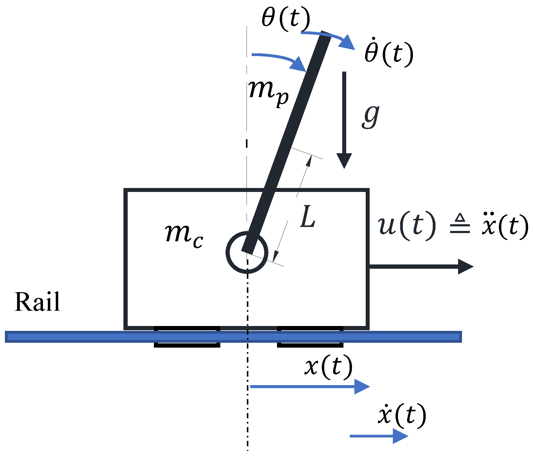
2.1. Cart Inverted Pendulum Dynamic

The CIP system consists of a cart moving along a rail, with a pendulum hinged to the cart, as shown in Figure 1. The displacement of the cart $x\left(t\right)$ (m) is considered in the horizontal direction and its velocity is denoted as $\dot{x}\left(t\right)$ (m/s). The angle between the pendulum and the vertical up direction is considered as the pendulum angle $\theta \left(t\right)$ (rad) and its angular velocity is $\dot{\theta }\left(t\right)$ (rad/s). The mass of the cart and of the pendulum are denoted by $m_c$ (kg) and $m_p$ (kg), respectively; L is the half-length of the pendulum (m); g is the gravitational constant (m/s²); and $u\left(t\right)$ is the required acceleration parallel to the rail, applied to the cart (m/s²). The required acceleration of the motor is controlled by a pulse-width-modulation (PWM) signal from a stepper driver.

The mathematical model of the CIP is derived under the following assumptions: [38]: (i) the pendulum of the CIP system is considered as a rigid body; (ii) during the experimental test, the length of the belt remained constant; (iii) there is no delay of the acceleration applied to the cart. According to these assumptions, a mathematical model of the CIP was derived based on the Lagrange equation. To employ the Lagrange method, the kinetic and potential energies of the cart and pendulum need to be computed and combined to the form of energy of the system.

The total kinetic energy of CIP is described as

$$T\triangleq {\displaystyle \frac{1}{2}}(m_c+m_p){\dot{x}}^2+m_{p}l\dot{x}\dot{\theta }cos\theta +{\displaystyle \frac{1}{2}}(I+m_p{l}^2){\dot{\theta }}^2.$$

(1)

Similarly, the total potential energy is expressed as follows:

$$\mathcal{V}\triangleq m_{p}gL(cos\left(\theta \left(t\right)\right)-1).$$

(2)

The Lagrangian for the CIP $\mathcal{L}\triangleq \mathcal{T}-\mathcal{V}$ is defined as the difference between the kinetic energy and the potential energy.

$$\begin{array}{c}\hfill \mathcal{L}={\displaystyle \frac{1}{2}}(m_c+m_p){\dot{x}}^2\left(t\right)+m_{p}L\dot{x}\left(t\right)\dot{\theta }\left(t\right)cos\left(\theta \left(t\right)\right)\\ \hfill +{\displaystyle \frac{1}{2}}(I+m_p{L}^2)\dot{\theta }{\left(t\right)}^2-m_{p}gL(cos\left(\theta \left(t\right)\right)-1).\end{array}$$

(3)

Finally, Lagrange’s equations, including non-conservative forces, result in [39]

$${\displaystyle \frac{{\partial }^2\mathcal{L}}{\partial t\partial \dot{\theta }}}-{\displaystyle \frac{\partial \mathcal{L}}{\partial \theta }}=-f_p\left(t\right),$$

(4)

where $f_p\left(t\right)$ is the viscous damping force of the pendulum:

$$f_p\left(t\right)\triangleq k_d\dot{\theta }\left(t\right),$$

(5)

where $k_d$ is the damping coefficient, determined by the free damped vibration of the pendulum:

$${\displaystyle \frac{\partial \mathcal{L}}{\partial \theta \left(t\right)}}=-m_{p}L\dot{x}\left(t\right)\dot{\theta }\left(t\right)sin\left(\theta \left(t\right)\right)+m_{p}gLsin\left(\theta \left(t\right)\right);$$

(6)

$${\displaystyle \frac{\partial \mathcal{L}}{\partial \dot{\theta }\left(t\right)}}=m_{p}L\dot{x}\left(t\right)cos\left(\theta \left(t\right)\right)+(I+m_p{L}^2)\dot{\theta }\left(t\right).$$

(7)

The dynamic model of the CIP can be represented as

$$m_{p}l\ddot{x}\left(t\right)cos\left(\theta \left(t\right)\right)+(I+m_p{L}^2)\ddot{\theta }\left(t\right)-m_{p}gLsin\left(\theta \left(t\right)\right)=-f_p\left(t\right).$$

(8)

When the control input of the CIP is the acceleration of the cart $u\left(t\right)\triangleq \ddot{x}\left(t\right)$, the overall model of the CIP can be described as follows:

$$\begin{array}{c}\hfill \ddot{\theta }\left(t\right)=-{\displaystyle \frac{k_d\dot{\theta }\left(t\right)}{(I+m_p{L}^2)}}-{\displaystyle \frac{m_{p}L(cos\theta \left(t\right))}{(I+m_p{L}^2)}}u\left(t\right)\\ \hfill +{\displaystyle \frac{m_{p}gLsin\left(\theta \left(t\right)\right)}{(I+m_p{L}^2)}}.\end{array}$$

(9)

2.2. Linearization

Although IP systems are inherently non-linear (9), they can be linearized when the pendulum operates in a small neighborhood around an unstable equilibrium point $(\theta \left(t\right),\dot{\theta }\left(t\right))=(0,0)$. This linearization process involves expanding the non-linear function into the Tailor series about the operation point and neglecting high-order terms of expansion [40]. The resulting linearized state space representation of the system around the unstable equilibrium point of the CIP is obtained as follows:

$$\dot{\mathbf{x}}\left(t\right)=\mathbf{A}\mathbf{x}\left(t\right)+\mathbf{b}u\left(t\right),$$

(10)

where $\mathbf{x}\left(t\right)\in {\mathbb{R}}^{4\times 1}$ is the state vector of the system

$$\mathbf{x}\left(t\right)\triangleq \left[\begin{array}{c}x\left(t\right)\\ \dot{x}\left(t\right)\\ \theta \left(t\right)\\ \dot{\theta }\left(t\right)\end{array}\right];$$

(11)

and the state space matrices are

$$\mathbf{A}\triangleq \left[\begin{array}{cccc}0& 1& 0& 0\\ 0& 0& 0& 0\\ 0& 0& 0& 1\\ 0& 0& {\displaystyle \frac{Lg{m}_p}{(m_p{L}^2+I)}}& -{\displaystyle \frac{k_d}{(m_p{L}^2+I)}}\end{array}\right];$$

(12)

$$\mathbf{b}\triangleq \left[\begin{array}{c}0\\ 1\\ 0\\ -{\displaystyle \frac{L{m}_p}{(m_p{L}^2+I)}}\end{array}\right].$$

(13)

In CIP systems, uncertainties stemming from inaccurate modeling and external disturbances are unavoidable. The lumped disturbance $\mathbf{f}(\mathbf{x}\left(t\right),u\left(t\right))\in {\mathbb{R}}^4$ is defined as the total value of uncertainties and external disturbances, assumed to be unknown but bounded by some known functions of the state. Therefore, the nominal CIP model (10) is rewritten in the presence of the lumped disturbances as follows:

$$\dot{\mathbf{x}}\left(t\right)=\mathbf{A}\mathbf{x}\left(t\right)+\mathbf{b}u\left(t\right)+\mathbf{f}(\mathbf{x}\left(t\right),u\left(t\right)).$$

(14)

Control objective: An augmented model, which includes the integral cart position errors, was designed to develop a sliding mode controller. This approach removes the offset of the cart position caused by pendulum angle calibration errors and ensures robustness against matched disturbances. The proposed control was experimentally verified to demonstrate its implementation capability and effectiveness for the stabilization and tracking problem of a CIP.

3. Integral Linear Quadratic Regulator Sliding Mode Control (ILQRSMC)

From the linear CIP model (14), the error dynamic model of the CIP can be obtained as follows:

$$\dot{\mathbf{e}}\left(t\right)=\mathbf{A}\mathbf{e}\left(t\right)+\mathbf{b}u\left(t\right)+\mathit{\varphi }\left(t\right),$$

(15)

where $\mathbf{e}\left(t\right)\triangleq \mathbf{x}\left(t\right)-{\mathbf{x}}_d\left(t\right)$ represents the error vector between the actual state vector $\mathbf{x}\left(t\right)$ and the desired state vector ${\mathbf{x}}_d\left(t\right)\triangleq {\left[x_d\left(t\right){\dot{x}}_d\left(t\right){\theta }_d\left(t\right){\dot{\theta }}_d\left(t\right)\right]}^T$; the total disturbance can be defined as $\mathit{\varphi }\left(t\right)\triangleq \mathbf{f}(\mathbf{x}\left(t\right),u\left(t\right))+\mathbf{A}{\mathbf{x}}_d\left(t\right)-{\dot{\mathbf{x}}}_d\left(t\right)$. To eliminate the steady-state errors of the cart position, the integral action of the cart position error is incorporated with the error model system (15) to construct a new augmented error model, given as

$${\dot{\mathbf{e}}}_g\left(t\right)={\mathbf{A}}_g{\mathbf{e}}_g\left(t\right)+{\mathbf{b}}_{g}u\left(t\right)+{\mathit{\varphi }}_g\left(t\right),$$

(16)

where

$${\mathbf{e}}_g\left(t\right)\triangleq \left[\begin{array}{c}x\left(t\right)-x_d\left(t\right)\\ \dot{x}\left(t\right)-{\dot{x}}_d\left(t\right)\\ \theta \left(t\right)-{\theta }_d\left(t\right)\\ \dot{\theta }\left(t\right)-{\dot{\theta }}_d\left(t\right)\\ \int x\left(t\right)-\int x_d\left(t\right)\end{array}\right];$$

(17)

$${\mathbf{A}}_g\triangleq \left[\begin{array}{ccccc}0& 1& 0& 0& 0\\ 0& 0& 0& 0& 0\\ 0& 0& 0& 1& 0\\ 0& 0& {\displaystyle \frac{Lg{m}_p}{(m_p{L}^2+I)}}& -{\displaystyle \frac{k_d}{(m_p{L}^2+I)}}& 0\\ 1& 0& 0& 0& 0\end{array}\right];$$

(18)

$${\mathbf{b}}_g\triangleq \left[\begin{array}{c}0\\ 1\\ 0\\ -{\displaystyle \frac{L{m}_p}{(m_p{L}^2+I)}}\\ 0\end{array}\right];$$

(19)

$${\mathit{\varphi }}_g\triangleq {\left[\mathit{\varphi }0\right]}^T.$$

(20)

The lumped disturbance ${\mathit{\varphi }}_g\left(t\right)$ comprises the matched lumped disturbance ${\varphi }_m$ and unmatched lumped disturbance ${\mathit{\varphi }}_u$, where each component can be determined as in proposition 1 in [41].

From [41], the lumped disturbance ${\mathit{\varphi }}_g$ can be projected into the column spaces of ${\mathbf{b}}_g$ and ${\mathbf{b}}_g^{\perp }$ to decompose it into matched ${\mathit{\varphi }}_m\left(t\right)$ and unmatched lumped disturbances ${\mathit{\varphi }}_u\left(t\right)$, as given by:

$${\mathit{\varphi }}_g\left(t\right)={\mathbf{b}}_g{\varphi }_m\left(t\right)+{\mathit{\varphi }}_u\left(t\right),$$

(21)

where ${\varphi }_m\left(t\right)={\mathbf{b}}_g^{+}\mathit{\varphi }\left(t\right)$, $\mathit{\varphi }u\left(t\right)={\mathbf{b}}_g^{\perp }{\mathbf{b}}_g^{\perp +}\mathit{\varphi }\left(t\right)$, ${\mathbf{b}}_g^{+}$ is left as the inverse of ${\mathbf{b}}_g$, and ${\mathbf{b}}_g^{\perp }$ is the null space of ${\mathbf{b}}_g^T$. Substituting the lumped disturbance ${\mathit{\varphi }}_g$ (21) into the augmented error (16) yields

$${\dot{\mathbf{e}}}_g\left(t\right)={\mathbf{A}}_g{\mathbf{e}}_g\left(t\right)+{\mathbf{b}}_g(u\left(t\right)+{\varphi }_m\left(t\right))+{\mathit{\varphi }}_u\left(t\right).$$

(22)

It is well known that the procedure for designing sliding mode control comprises two main steps: sliding surface design to achieve the desired performance in the sliding mode, and sliding mode control design to ensure the system trajectories converge to the sliding surface [42]. A linear sliding surface [29] $s\left({\mathbf{e}}_g\right)\in \begin{array}{c}\hfill R\end{array}$ is considered in this work, given as follows:

$$s\left({\mathbf{e}}_g\right)\triangleq \mathbf{c}{\mathbf{e}}_g\left(t\right),$$

(23)

where $\mathbf{c}\triangleq \left[c_1{c}_2{c}_3{c}_4{c}_5\right]$ is the design vector that is selected based on the system performance specifications. The proposed sliding mode controller $u\left(t\right)\in R$ consists of two components, defined as follows:

$$u\left(t\right)\triangleq u_0\left(t\right)+u_1\left(t\right),$$

(24)

where $u_0\left(t\right)=-{\left(\mathbf{c}{\mathbf{b}}_g\right)}^{-1}\left(\mathbf{c}{\mathbf{A}}_g{\mathbf{e}}_g\left(t\right)\right)$ can be obtained by solving $\dot{s}\left({\mathbf{e}}_g\right)\equiv 0$ without the lumped disturbance ${\mathit{\varphi }}_g$ in (16) [43], and $u_1\left(t\right)$ in (24) is designed as in [44], in order to mitigate the chattering problem:

$$\dot{s}\left({\mathbf{e}}_g\right)=-k_{sw}{\left|s\left({\mathbf{e}}_g\right)\right|}^{\alpha }\mathrm{sgn}\left(s\left({\mathbf{e}}_g\right)\right),0<\alpha <1,$$

(25)

where $k_{sw}$ is a positive design parameter, and

$$\mathrm{sgn}\left(s\left({\mathbf{e}}_g\right)\right)=\left\{\begin{array}{c}1\mathrm{if}s\left({\mathbf{e}}_g\right)>0,\hfill \\ 0\mathrm{if}s\left({\mathbf{e}}_g\right)=0,\hfill \\ -1\mathrm{if}s\left({\mathbf{e}}_g\right)<0.\hfill \end{array}\right.$$

As shown in (25), the reaching speed is adjusted based on the distance of the system states from the sliding surface. When the system states are far from the sliding surface, the reaching speed increases. Conversely, when the system states approach the sliding surface, the reaching speed decreases, effectively mitigating overshoot and chattering of control input. The term ${\left|s\left(t\right)\right|}^{\alpha }$ plays an important role in mitigating the chattering problem. However, selecting an appropriate value of $\alpha$ involves a trade-off: higher values improve chattering reduction, but they may compromise controller robustness.

When the system is in sliding mode $s\left({\mathbf{e}}_g\right)=0$ and $\dot{s}\left({\mathbf{e}}_g\right)=0$, its motion in sliding mode can be explained by using an equivalent control technique, which represents the average control action required to maintain the system on the sliding surface [42]. The equivalent control $u_{eq}\left(t\right)$ can be obtained by solving $u\left(t\right)$ for the time derivative of the sliding surface $\dot{s}\left({\mathbf{e}}_g\right)\equiv 0$.

$$\begin{array}{c}\hfill \dot{s}\left({\mathbf{e}}_g\right)=\mathbf{c}({\mathbf{A}}_g{\mathbf{e}}_g\left(t\right)+{\mathbf{b}}_g(u\left(t\right)+{\varphi }_m\left(t\right))+{\mathit{\varphi }}_u\left(t\right))\equiv 0,\forall t\ge t_s\\ \hfill u_{eq}=-{\left(\mathbf{c}{\mathbf{b}}_g\right)}^{-1}\mathbf{c}\left({\mathbf{A}}_g{\mathbf{e}}_g+{\mathbf{b}}_g{\varphi }_m\left(t\right)+{\mathit{\varphi }}_u\left(t\right)\right).\end{array}$$

(26)

Substituting (26) for $u\left(t\right)$ into (22), the sliding model dynamic is

$${\dot{\mathbf{e}}}_g\left(t\right)=\left(\mathbf{I}-{\mathbf{b}}_g{\left(\mathbf{c}{\mathbf{b}}_g\right)}^{-1}\mathbf{c}\right){\mathbf{A}}_g{\mathbf{e}}_g\left(t\right)+\left(\mathbf{I}-{\mathbf{b}}_g{\left(\mathbf{c}{\mathbf{b}}_g\right)}^{-1}\mathbf{c}\right){\mathit{\varphi }}_u\left(t\right),\forall t\ge t_s.$$

(27)

It can be observed that the sliding mode dynamic (27) does not contain the matched disturbance, showing the properties of SMC in rejecting matched disturbances. However, unmatched disturbances are multiplied by $\mathbf{\Gamma }\triangleq (\mathbf{I}-{\mathbf{b}}_g{\left(\mathbf{c}{\mathbf{b}}_g\right)}^{-1}\mathbf{c})$. Furthermore, the sliding mode dynamic does not depend on the control input; however, it depends on the selection of the value $\mathbf{c}$ of the sliding surface $s\left({\mathbf{e}}_g\right)$. Since the values of $\mathbf{c}$ significantly affect the performance of the sliding mode dynamic, selecting $\mathbf{c}$ should be carried out carefully to avoid amplifying unmatched disturbances. Therefore, $\mathbf{c}$ is selected to avoid amplifying unmatched disturbances ${\mathit{\varphi }}_u$ in (22), as thoroughly analyzed by [41]. As a result, the sliding mode dynamic can be simplified as follows:

$${\dot{\mathbf{e}}}_g\left(t\right)=\left({\mathbf{A}}_g-{\mathbf{b}}_g\mathbf{k}\right){\mathbf{e}}_g\left(t\right)+\left(\mathbf{I}-{\mathbf{b}}_g\mathbf{c}\right){\mathit{\varphi }}_u\left(t\right),$$

(28)

where $\mathbf{k}\triangleq \mathbf{c}{\mathbf{A}}_g\in {\mathbb{R}}^{1\times 5}$. Linear control methods can be employed to solve for $\mathbf{k}$ such as LMI, pole placement, or LQR. In this work, $\mathbf{k}$ is determined using the LQR method, given by [17]

$$\mathbf{k}={\mathbf{R}}^{-1}{\mathbf{b}}_g^T\mathbf{P},$$

(29)

where $\mathbf{P}$ is solved from the Riccati equation

$${\mathbf{A}}_g^T\mathbf{P}+{\mathbf{PA}}_g+\mathbf{Q}-{\mathbf{Pb}}_g{\mathbf{R}}^{-1}{\mathbf{b}}_g^T\mathbf{P}=0,$$

(30)

where $\mathbf{Q}$ represents the state weighting matrix and $\mathbf{R}$ is the control weighting matrix. This equation can be solved using the MATLAB R2021b function care. From the selection $\mathbf{c}={\mathbf{b}}_g^{+}$ [45] and $\mathbf{k}\triangleq \mathbf{c}{\mathbf{A}}_g$ [43], the value of $\mathbf{c}$ should satisfy the following condition:

$$\mathbf{c}\left[{\mathbf{A}}_g{\mathbf{b}}_g\right]=\left[\mathbf{k}\mathbf{I}\right].$$

(31)

The solution of $\mathbf{c}$ can be directly determined by [46]

$$\mathbf{c}=\left[\mathbf{k}\mathbf{I}\right]{\left[{\mathbf{A}}_g{\mathbf{b}}_g\right]}^{+},$$

(32)

where ${\left[{\mathbf{A}}_g{\mathbf{b}}_g\right]}^{+}$ is pseudo inverse.

The time derivative of the Lyapunov function $V\left(t\right)\triangleq s{\left({\mathbf{e}}_g\right)}^2/2$ is:

$$\dot{V}\left(t\right)=s\left({\mathbf{e}}_g\right)\dot{s}\left({\mathbf{e}}_g\right).$$

(33)

Substituting the control input (24) into the time derivative of $s\left({\mathbf{e}}_g\right)$ (26) yields

$$\dot{s}\left({\mathbf{e}}_g\right)=-k_{sw}{\left|s\left({\mathbf{e}}_g\right)\right|}^{\alpha }sgn\left(s\left({\mathbf{e}}_g\right)\right)+{\varphi }_m\left(t\right)+\mathbf{c}{\mathit{\varphi }}_u\left(t\right).$$

(34)

Therefore,

$$\dot{V}\left(t\right)=-k_{sw}{\left|s\left({\mathbf{e}}_g\right)\right|}^{\alpha +1}+s({\varphi }_m\left(t\right)+\mathbf{c}{\mathit{\varphi }}_u\left(t\right)).$$

(35)

Selecting $k_{sw}\ge |({\varphi }_m+\mathbf{c}{\mathit{\varphi }}_u)/\left(s{\left({\mathbf{e}}_g\right)}^{\alpha }\right)|$, we have $\dot{V}\left(t\right)\le 0$, $s\left({\mathbf{e}}_g\right)\to 0$, ${\mathbf{e}}_g\left(t\right)\to 0$.

 Remark 1. 

To implement the proposed control, it is necessary to have advance knowledge of the system states $x\left(t\right),\dot{x}\left(t\right),\theta \left(t\right),\dot{\theta }\left(t\right)$. However, in most practical IP systems, only the position of the cart or pendulum can be measured by encoder sensors. Therefore, $\dot{x}\left(t\right),\dot{\theta }\left(t\right)$ need to be estimated by alternative approaches. In this work, for the sake of simplifying the control algorithm, $\dot{x}\left(t\right),\dot{\theta }\left(t\right)$ are determined using a numerical derivative with a low-pass filter. This approach helps mitigate the effect of noise in the measurement process [47].

The design procedure for the proposed control can be formulated as follows:

• Select the matrices $\mathbf{Q}$ and $\mathbf{R}$ to solve the Riccati Equation (30).
• Determine the value of $\mathbf{k}$ from (29), then determine $\mathbf{c}$ from (32).
• Solve $\mathbf{c}$ from (32), then determine the sliding surface $s\left({\mathbf{e}}_g\left(t\right)\right)$ from (23).
• Calculate $u_0\left(t\right)=-{\left(\mathbf{c}{\mathbf{b}}_g\right)}^{-1}\left(\mathbf{c}{\mathbf{A}}_g{\mathbf{e}}_g\left(t\right)\right)$, and $u_1\left(t\right)$ (25), then determine $u\left(t\right)$ (24).

4. Experimental Results

4.1. Experimental Setup

To evaluate the effectiveness of the proposed control for CIPs, experimental studies were carried out on a CIP prototype, developed at the Department of Mechanics of Adaptive Systems, Ruhr University Bochum, as shown in Figure 2. A stepper motor ① Sanyo denki 103h7123-5040, SANYO DENKI, Osaka, Japan was used to exert acceleration on the cart ② determined by the proposed controller. The angle position of the pendulum was measured directly by the rotary magnetic encoder module ③ RMB28AC, A RENISHAW associate company, Wotton-under-Edge, UK with a resolution 1024 counts/rev installed at the end of pendulum ④. A miniature incremental magnetic encoder module ⑤ RLC2HD, RLS, Komenda, Slovenia with a resolution of 80,000 counts/m was attached to the cart to measure its position along the magnetic scale ⑥. In this system, a stepper motor transfers the power to the cart by pulling the belt ⑦ in two directions and inducing its movements. The signals obtained by a rotary magnetic encoder and miniature incremental magnetic encoder are transmitted to dSPACE ⑧ Scalexio with a sampling time of $0.001\mathrm{s}$. The acceleration exerted on the cart, calculated by the proposed controller, is converted to pulse width modulation (PWM) [48] and provided to a microstep driver ⑨ of the stepper motor via dSPACE Scalexio. In the experimental scenario, the physical parameters included the gravitational constant g = 9.8 m/s²; the mass of the cart $m_c$ = 0.8 kg; the mass of the pendulum $m_p$ = 0.188 kg; and the half-length of the pendulum L = 0.34 m. Several nuts ⑩ were attached to the tip of the pendulum, considered as an unknown lumped disturbance on the CIP. The initial pendulum angle could be adjusted by employing a pendulum clamp ⑪. The initial conditions of the CIP were set as $\mathbf{x}\left(t_0\right)={\left[0.03600.1240\right]}^T$. For the sake of comparing controller performance, integral linear quadratic regulator (ILQR) control [49] was reproduced. The ILQR was designed as follows [16]:

$$u_{\mathrm{ILQR}}\left(t\right)\triangleq -{\mathbf{R}}^{-1}{\mathbf{b}}_g^T\mathbf{P}{\mathbf{e}}_g\left(t\right),$$

(36)

where $\mathbf{P}$ is a symmetric positive definite matrix that is the solution of the algebraic Riccati (30). The primary control parameters of the ILQR and the proposed control are listed in

Table 1. Parameter settings of each controller for stabilization and tracking control of the cart inverted pendulum.

Controller	Tuning Parameters
ILQR	$\mathbf{R}=1;\mathbf{Q}=0.01\mathrm{diag}\left[10.150.210\right]$.
Proposed control	$\mathbf{R}=1;\mathbf{Q}=0.01\mathrm{diag}\left[10.150.210\right];k_{sw}=1;\alpha =0.7$.

.

4.2. Experimental Results

In order to verify the effectiveness of the proposed control, two sets of experimental results are given in this section, which can be found at https://drive.google.com/drive/u/1/folders/1EDfmfJO6DxuiMBsBjOm-bS_dUSDOJui4 (accessed on 6 April 2025). The first experiment demonstrated the stabilization of the CIP under its own mechanical disturbances and small errors of the cart position and pendulum angle. The second experiment showcased the tracking performance of cart position of the CIP while maintaining the balance of pendulum. It should be noted that the swing up procedure was not utilized in these experiments and the initial conditions of the CIP were set manually.

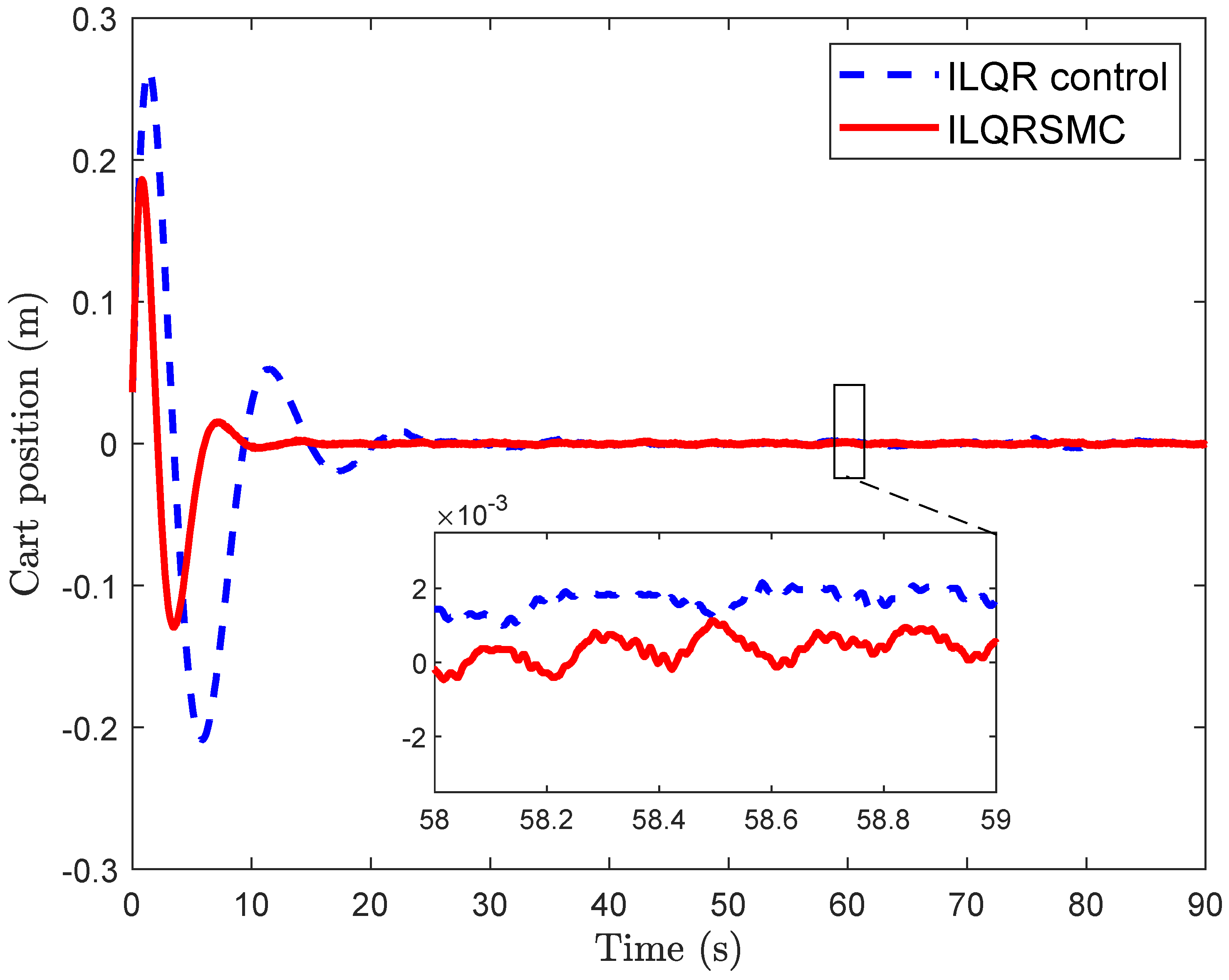
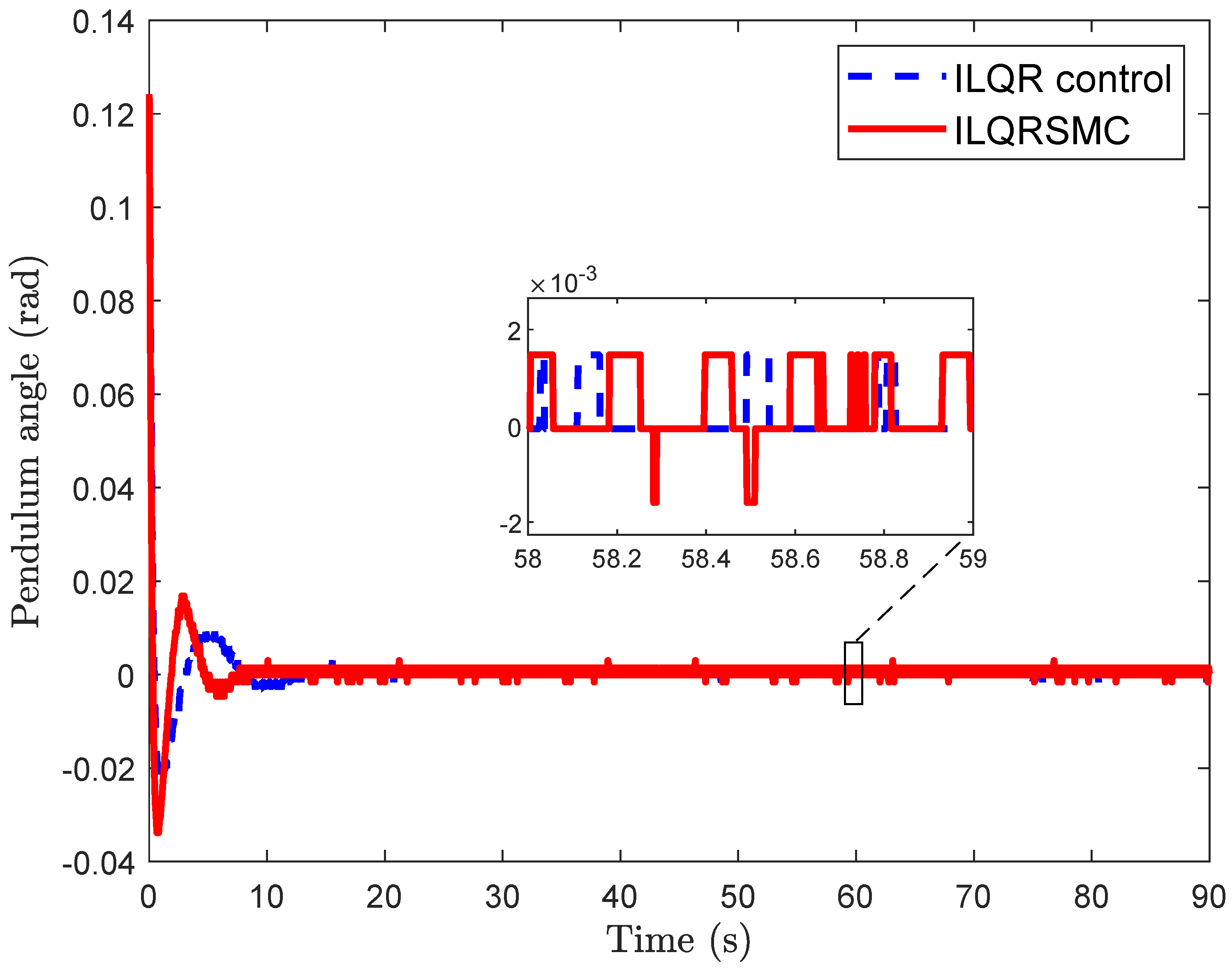
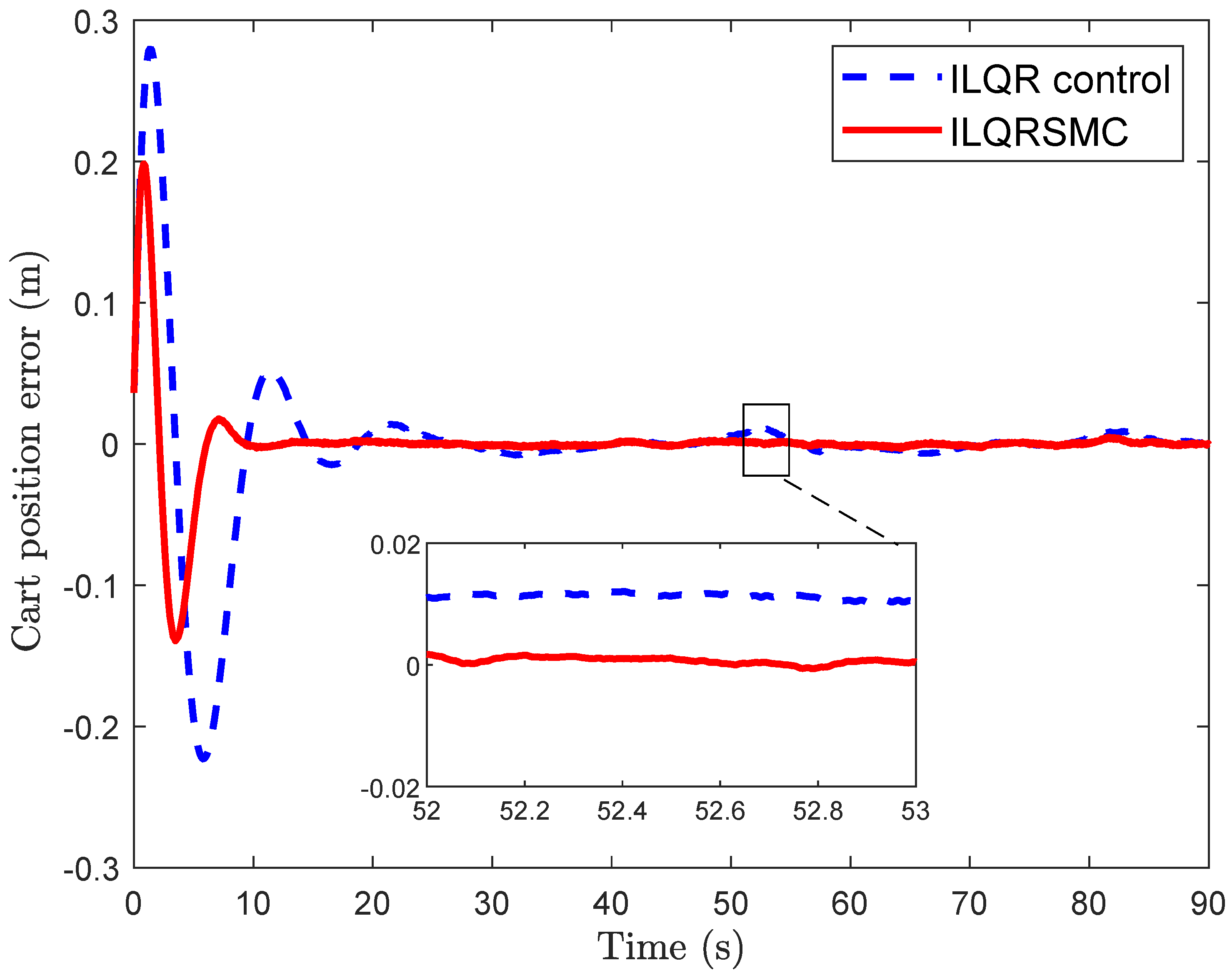
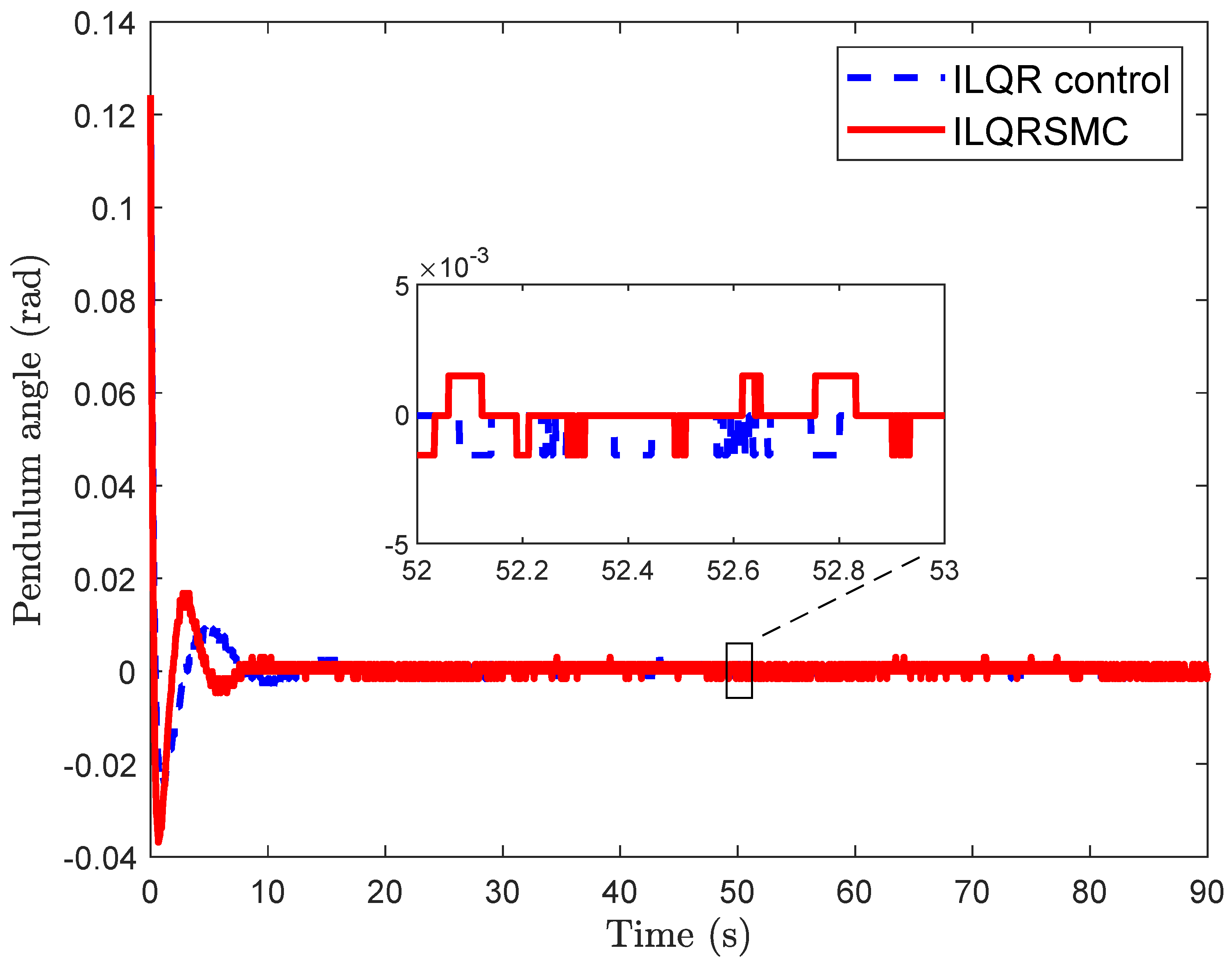
4.2.1. Stabilization Control of Cart Inverted Pendulum

The stabilization control aimed to stabilize the pendulum in the upright position ${\theta }_d\left(t\right)$ = 0 rad starting from a small initial angle, while simultaneously maintaining the cart position around the desired position $x_d\left(t\right)=0$ m.

The experimental results represented in Figure 3 and Figure 4 show a performance comparison between the ILQR and the proposed controller in terms of the cart position and the pendulum angle. Although both controllers could ensure the balance of the CIP with a small initial angle of pendulum $\theta \left(0\right)=0.124$ rad, the cart position plots in Figure 3 reveal notable differences in their performance. While the ILQR generated large cart position errors of about $0.26$ m at the beginning of the response, the proposed controller exhibited smaller errors and less oscillation, reducing overshoot by about $30\%$. After $25$ s, ILQR achieved a satisfactory performance, as demonstrated by the small cart position errors that remained close to zero. In contrast, the proposed controller settled within this threshold in approximately $10$ s, showing a $60\%$ improvement in convergence speed. Both the proposed control and the ILQR achieved small steady-state tracking errors for the cart position of round $2\times {10}^{-3}$ m. However, the peak overshoot of the cart position was substantially diminished, from $0.26$ m to $0.18$ m, in the proposed control. Similarly, the undershoot of the cart position in the proposed control was smaller, with a value of $-0.12$ m, compared to $-0.2$ m in the ILQR. Moreover, as can be seen from Figure 4, both ILQR and the proposed control demonstrated rapid responses, to bring the pendulum from an initial error to its upright position after $10$ s. As can be seen from the zoomed part of the steady-state response, while the steady-state error was kept within the range of $-0.001$ rad $\sim 0.001$ rad in both cases, the proposed control demonstrated superior performance compared to the ILQR in the 0–10 s interval.

For a more comprehensive qualitative analysis,

Table 2. Index values of control strategies for stabilization control.

	IAE of Cart Position (m)	IAE of Pendulum Angle (rad)	IAC
ILQR	1.6714	0.1209	7.8814
Proposed control	0.6233	0.1292	16.0692

provides the index values of the integrated absolute error (IAE) of the cart position error and the pendulum angle error. These indexes are defined from [50]:

$${\mathrm{IAE}}_x={\int }_0^T|x\left(t\right)-x_d\left(t\right)|dt,$$

(37)

$${\mathrm{IAE}}_{\theta }={\int }_0^T|\theta \left(t\right)-{\theta }_d\left(t\right)|dt,$$

(38)

where T is the running time, ${\mathrm{IAE}}_x$ and ${\mathrm{IAE}}_{\theta }$ are the integrated absolute error of the cart position error and the pendulum angle error, respectively. Smaller IAE values signify better tracking performance, as they reflect less accumulation of tracking errors. In contrast, higher values of IAE imply a greater accumulation of tracking errors, thereby indicating a worse tracking capability. In this context, the proposed control exhibited an ${\mathrm{IAE}}_x$ index of $0.6233$ m for cart position, while this index for ILQR was $1.6714$ m. The time change of IAE_x is given in Figure 5, indicating the fast error convergence and small steady-state error of the proposed control. The proposed control achieved a slightly higher ${\mathrm{IAE}}_{\theta }$ index value for pendulum angle at $0.1292$ rad, which can be attributed to the transient response from 0–10s. To thoroughly evaluate the control performance of a CIP system, it is necessary to separately analyze the IAE_x and ${\mathrm{IAE}}_{\theta }$ values. By comparing the ${\mathrm{IAE}}_x$, ${\mathrm{IAE}}_{\theta }$ values, which present the total accumulated errors in the cart position and pendulum angle over time, respectively, a detailed understanding about the dynamic behaviors of the cart motion and pendulum angle can be obtained. Furthermore, to evaluate the overall performance of the CIP for each controller, the total IAE index value is calculated by combining the ${\mathrm{IAE}}_x$ and ${\mathrm{IAE}}_{\theta }$ values. The total integrated absolute error of both the cart and pendulum angle error of the proposed control was $0.7525$, significantly lower than the $1.7923$ recorded for the ILQR control, indicating the superior performance of the proposed control method. Although the proposed control provided good stabilization performance for the CIP, its control signal was higher than that of the ILQR controller, as shown in Figure 6. This can be explained by the structure of the SMC control law, which consists of a linear component $u_0\left(t\right)$ and discontinuous component $u_1\left(t\right)$. The linear term $u_0\left(t\right)$ stabilizes the nominal system, while the discontinuous term $u_1$ compensates for the matched lumped disturbance. By contrast, the low control signal of the ILQR may result in an inadequate control input for the CIP, reducing its ability to effectively counteract disturbances and uncertainties [51]. Although the control input plots demonstrate a qualitative comparison of these controllers, a comprehensive evaluation could be conducted by quantifying the control effort. One such quantitative measure is the integral absolute control (IAC) [52], which calculates the total absolute value of the control signal over time and is determined as follows:

$$\mathrm{IAC}={\int }_0^T\left|u\left(t\right)\right|dt.$$

(39)

This metric reflects the control effort, where smaller values indicate more energy-efficient control. From Table 2, the proposed control exhibited a higher value of IAC compared to the ILQR control, indicating that it required a greater control effort to compensate for the lumped disturbance.

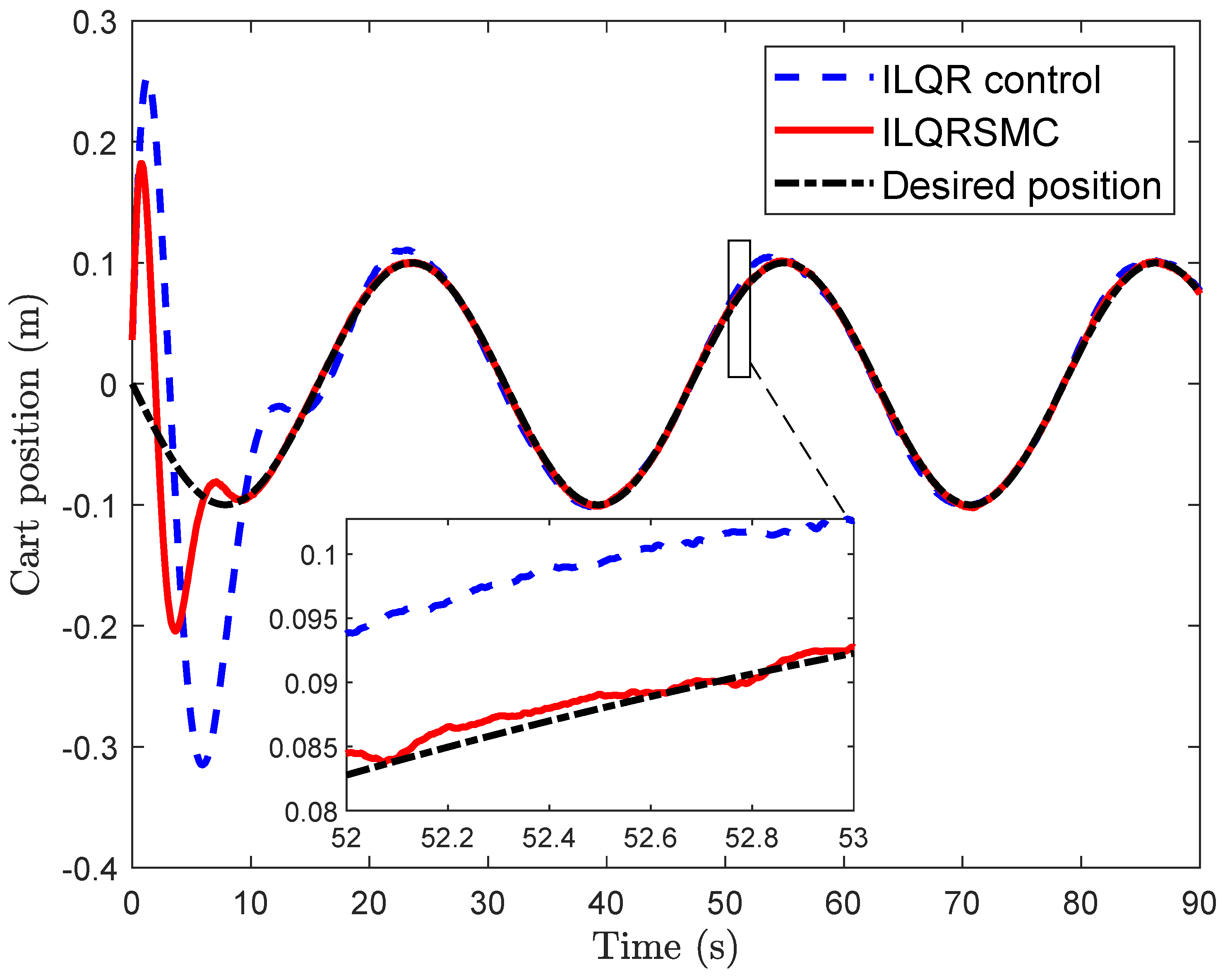
4.2.2. Tracking Control of Cart Inverted Pendulum

In this case, to verify the tracking performance of the CIP, a smooth desired cart position $x_d\left(t\right)=0.1sin\left(0.2t\right)$ was utilized while maintaining the pendulum tightly around the upright position. Both controllers enabled the CIP to track the desired cart position after different transition times, as depicted in Figure 7. In Figure 8, the cart position errors for the ILQR and the proposed controller are shown. From 0 to 20 s, the proposed control generated smaller cart position errors compared to the ILQR, reaching the desired position within about $10$ s, as opposed to $27$ s with the ILQR. Upon closer examination of the cart position errors, the proposed control achieved smaller errors than the ILQR control, demonstrating a $50\%$ reduction in errors. Similarly, the pendulum angle of the proposed control during the 0–10 s interval showed better performance than the ILQR control, given in Figure 9. Furthermore, the proposed control demonstrated superior tracking performance for the cart position errors, as evidenced by the smaller IAE values, as shown in

Table 3. Index values of control strategies in tracking control.

	IAE of Cart Position (m)	IAE of Pendulum Angle (rad)	IAC
ILQR	1.9151	0.1303	7.5683
Proposed control	0.7005	0.1348	15.3816

. The evolution of IAE_x given in Figure 10 highlights the robustness and effectiveness of the proposed controller in handling lumped disturbances, outperforming the ILQR controller. Although the control input of the proposed control was slightly higher than that of the ILQR control, it provided superior tracking performance for the CIP, as demonstrated in Figure 11. While the ILQR achieved a low energy consumption compared to our approach, this came at the cost of increased cart position errors in the CIP.

5. Conclusions

In this article, a new optimal sliding mode control with integral action was proposed for an inverted pendulum, to solve the balancing and tracking problem. The proposed control was evaluated and compared with an ILQR control in experimental studies in two scenarios. The results indicate that the proposed method effectively alleviated overshoot at the beginning of the transient response and improved the tracking accuracy of the cart and pendulum position. Future works will involve combining an ${\mathrm{H}}_{\infty }$ controller to reduce the effect of unmatched disturbances. In addition, exploring a higher-order sliding mode to effectively minimize the chattering control signal will be also considered.

References

1. Emran, B.J.; Najjaran, H. A review of quadrotor: An underactuated mechanical system. Annu. Rev. Control 2018, 46, 165–180. [Google Scholar] [CrossRef]
2. Kumar, E.V.; Jerome, J. Robust LQR controller design for stabilizing and trajectory tracking of inverted pendulum. Procedia Eng. 2013, 64, 169–178. [Google Scholar] [CrossRef]
3. Boubaker, O.; Iriarte, R. The Inverted pendulum in Control Theory and Robotics: From Theory to New Innovations; Technical Report; IET: Stevenage, UK, 2017. [Google Scholar]
4. Boubaker, O. The inverted pendulum benchmark in nonlinear control theory: A survey. Int. J. Adv. Robot. Syst. 2013, 10, 233. [Google Scholar] [CrossRef]
5. Wang, J.J. Stabilization and tracking control of X–Z inverted pendulum with sliding-mode control. ISA Trans. 2012, 51, 763–770. [Google Scholar] [CrossRef]
6. Dwivedi, P.; Pandey, S.; Junghare, A.S. Stabilization of unstable equilibrium point of rotary inverted pendulum using fractional controller. J. Frankl. Inst. 2017, 354, 7732–7766. [Google Scholar] [CrossRef]
7. Saleem, O.; Mahmood-Ul-Hasan, K. Indirect adaptive state-feedback control of rotary inverted pendulum using self-mutating hyperbolic-functions for online cost variation. IEEE Access 2020, 8, 91236–91247. [Google Scholar] [CrossRef]
8. Yang, Y.; Zhang, H.H.; Voyles, R.M. Optimal fractional-order proportional–integral–derivative control enabling full actuation of decomposed rotary inverted pendulum system. Trans. Inst. Meas. Control 2023, 45, 1986–1998. [Google Scholar] [CrossRef]
9. Yang, X.; Zheng, X. Swing-up and stabilization control design for an underactuated rotary inverted pendulum system: Theory and experiments. IEEE Trans. Ind. Electron. 2018, 65, 7229–7238. [Google Scholar] [CrossRef]
10. Abdullah, M.; Amin, A.A.; Iqbal, S.; Mahmood-ul Hasan, K. Swing up and stabilization control of rotary inverted pendulum based on energy balance, fuzzy logic, and LQR controllers. Meas. Control 2021, 54, 1356–1370. [Google Scholar] [CrossRef]
11. Chacko, S.J.; Abraham, R.J. On LQR controller design for an inverted pendulum stabilization. Int. J. Dyn. Control 2023, 11, 1584–1592. [Google Scholar] [CrossRef]
12. Maciejowski, J.M. Multivariable Feedback Design; Electronic Systems Engineering Series; Addison-Wesley: Boston, MA, USA, 1989. [Google Scholar]
13. Safonov, M.; Athans, M. Gain and phase margin for multiloop LQG regulators. IEEE Trans. Autom. Control 1977, 22, 173–179. [Google Scholar] [CrossRef]
14. Mahapatra, C.; Chauhan, S. Tracking control of inverted pendulum on a cart with disturbance using pole placement and LQR. In Proceedings of the 2017 International Conference on Emerging Trends in Computing and Communication Technologies (ICETCCT), Dehradun, India, 17–18 November 2017; pp. 1–6. [Google Scholar]
15. Chantarachit, S. Development and Control of Rotary Inverse Pendulum by LQR with Integral Action. IOP Conf. Ser. Mater. Sci. Eng. 2019, 639, 012022. [Google Scholar] [CrossRef]
16. Dai Le, H.; Nestorović, T. Integral Linear Quadratic Regulator for Inverted Pendulum System Actuated by a Step Motor. In Proceedings of the 2024 10th International Conference on Control, Decision and Information Technologies (CoDIT), Valetta, Malta, 1–4 July 2024; pp. 367–370. [Google Scholar]
17. Malkapure, H.G.; Chidambaram, M. Comparison of two methods of incorporating an integral action in linear quadratic regulator. IFAC Proc. Vol. 2014, 47, 55–61. [Google Scholar] [CrossRef]
18. Baumann, W.; Rugh, W. Feedback control of nonlinear systems by extended linearization. IEEE Trans. Autom. Control 1986, 31, 40–46. [Google Scholar] [CrossRef]
19. Utkin, V. Variable structure systems with sliding modes. IEEE Trans. Autom. Control 1977, 22, 212–222. [Google Scholar] [CrossRef]
20. Zhao, H.; Zong, G.; Zhao, X.; Wang, H.; Xu, N.; Zhao, N. Hierarchical Sliding-Mode Surface-Based Adaptive Critic Tracking Control for Nonlinear Multiplayer Zero-Sum Games Via Generalized Fuzzy Hyperbolic Models. IEEE Trans. Fuzzy Syst. 2023, 31, 4010–4023. [Google Scholar] [CrossRef]
21. Wang, W.; Yi, J.; Zhao, D.; Liu, D. Design of a stable sliding-mode controller for a class of second-order underactuated systems. IEE Proc.Control Theory Appl. 2004, 151, 683–690. [Google Scholar] [CrossRef]
22. Hwang, C.L.; Chiang, C.C.; Yeh, Y.W. Adaptive fuzzy hierarchical sliding-mode control for the trajectory tracking of uncertain underactuated nonlinear dynamic systems. IEEE Trans. Fuzzy Syst. 2013, 22, 286–299. [Google Scholar] [CrossRef]
23. Hwang, C.L.; Wu, H.M. Trajectory tracking of a mobile robot with frictions and uncertainties using hierarchical sliding-mode under-actuated control. IET Control Theory Appl. 2013, 7, 952–965. [Google Scholar] [CrossRef]
24. Yue, S.; Niu, B.; Wang, H.; Zhang, L.; Ahmad, A.M. Hierarchical sliding mode-based adaptive fuzzy control for uncertain switched under-actuated nonlinear systems with input saturation and dead-zone. Robot. Intell. Autom. 2023, 43, 523–536. [Google Scholar] [CrossRef]
25. Yan, M.-X.; Jing, Y.-W. Terminal sliding mode decomposed control for a class of nonlinear systems. In Proceedings of the 2008 Chinese Control and Decision Conference, Yantai, China, 2–4 July 2008; pp. 4988–4991. [Google Scholar]
26. Bayramoglu, H.; Komurcugil, H. Nonsingular decoupled terminal sliding-mode control for a class of fourth-order nonlinear systems. Commun. Nonlinear Sci. Numer. Simul. 2013, 18, 2527–2539. [Google Scholar] [CrossRef]
27. Edwards, C.; Shtessel, Y.B. Adaptive continuous higher order sliding mode control. Automatica 2016, 65, 183–190. [Google Scholar] [CrossRef]
28. Le, H.D.; Nestorović, T. A Novel Hierarchical Recursive Nonsingular Terminal Sliding Mode Control for Inverted Pendulum. Actuators 2023, 12, 462. [Google Scholar] [CrossRef]
29. Utkin, V. Methods for constructing discontinous planes in multidimensional variable structure systems. Autom. Remote Control 1977, 31, 1466–1470. [Google Scholar]
30. Edwards, C. A practical method for the design of sliding mode controllers using linear matrix inequalities. Automatica 2004, 40, 1761–1769. [Google Scholar] [CrossRef]
31. Pang, H.P.; Tang, G.Y. Optimal Sliding Manifold Design for Nonlinear Systems Based on Sensitivity Approach. In Proceedings of the 2006 IEEE International Conference on Systems, Man and Cybernetics, Taipei, Taiwan, 8–11 October 2006; Volume 2, pp. 1371–1376. [Google Scholar]
32. Patil, M.; Kurode, S. Stabilization of RDIP using sliding modes. In Proceedings of the 2018 Indian Control Conference (ICC), Kanpur, India, 4–6 January 2018; pp. 119–124. [Google Scholar]
33. Singh, S.; Swarup, A. Control of Rotary Double Inverted Pendulum using Sliding Mode Controller. In Proceedings of the 2021 International Conference on Intelligent Technologies (CONIT), Hubli, India, 25–27 June 2021; pp. 1–6. [Google Scholar]
34. Lu, B.; Fang, Y. Online trajectory planning control for a class of underactuated mechanical systems. IEEE Trans. Autom. Control 2023, 69, 442–448. [Google Scholar] [CrossRef]
35. Block, D.; Astrom, K.; Spong, M. The Reaction Wheel Pendulum; Morgan & Claypool Publishers: San Rafael, CA, USA, 2007. [Google Scholar]
36. Dotoli, M.; Maione, B.; Naso, D.; Turchiano, B. Fuzzy sliding mode control for inverted pendulum swing-up with restricted travel. In Proceedings of the 10th IEEE International Conference on Fuzzy Systems (Cat. No. 01CH37297), Melbourne, Australia, 2–5 December 2001; Volume 2, pp. 753–756. [Google Scholar]
37. Li, T.H.S.; Shieh, M.Y. Switching-type fuzzy sliding mode control of a cart–pole system. Mechatronics 2000, 10, 91–109. [Google Scholar] [CrossRef]
38. Furuta, K.; Kajiwara, H.; Kosuge, K. Digital control of a double inverted pendulum on an inclined rail. Int. J. Control 1980, 32, 907–924. [Google Scholar] [CrossRef]
39. Goldstein, H.; Poole, C.; Safko, J. Classical Mechanics; Addison and Wesley: San Francisco, CA, USA, 2003. [Google Scholar]
40. Ogata, K. Modern Control Engineering, 5th ed.; Pearson: London, UK, 2010. [Google Scholar]
41. Castanos, F.; Fridman, L. Analysis and design of integral sliding manifolds for systems with unmatched perturbations. IEEE Trans. Autom. Control 2006, 51, 853–858. [Google Scholar] [CrossRef]
42. Utkin, V.I. Sliding Modes in Control and Optimization; Springer Science & Business Media: Berlin/Heidelberg, Germany, 2013. [Google Scholar]
43. Chen, Y.P.; Chang, J.L. A new method for constructing sliding surfaces of linear time-invariant systems. Int. J. Syst. Sci. 2000, 31, 417–420. [Google Scholar] [CrossRef]
44. Gao, W. Variable structure control of nonlinear systems: A new approach. IEEE Trans. Ind. Electron. 1993, 40, 45–55. [Google Scholar]
45. Fridman, L.; Poznyak, A.; Bejarano, F.J. Robust Output LQ Optimal Control Via Integral Sliding Modes; Springer: New York, NY, USA, 2014. [Google Scholar]
46. Draženović, B.; Milosavljević, Č.; Veselić, B. Comprehensive approach to sliding mode design and analysis in linear systems. In Advances in Sliding Mode Control: Concept, Theory and Implementation; Springer: Berlin/Heidelberg, Germany, 2013; pp. 1–19. [Google Scholar]
47. Le, H.D.; Nestorović, T. Adaptive Proportional Integral Derivative Nonsingular Dual Terminal Sliding Mode Control for Robotic Manipulators. Dynamics 2023, 3, 656–677. [Google Scholar] [CrossRef]
48. Wang, B.; Liu, Q.; Zhou, L.; Zhang, Y.; Li, X.; Zhang, J. Velocity profile algorithm realization on FPGA for stepper motor controller. In Proceedings of the 2011 2nd International Conference on Artificial Intelligence, Management Science and Electronic Commerce (AIMSEC), Dengfeng, China, 8–10 August 2011; pp. 6072–6075. [Google Scholar]
49. Apkarian, J.; Lacheray, H.; Martin, P. Linear inverted pendulum experiment for matlab/simulink users. Quanser Student Workbook; Quanser Inc.: Markham, ON, Canada, 2012. [Google Scholar]
50. Yu, L.; He, G.; Wang, X.; Zhao, S. Robust fixed-time sliding mode attitude control of tilt trirotor UAV in helicopter mode. IEEE Trans. Ind. Electron. 2021, 69, 10322–10332. [Google Scholar] [CrossRef]
51. Mohd Haziq Norsahperi, N.; A Danapalasingam, K. A comparative study of LQR and integral sliding mode control strategies for position tracking control of robotic manipulators. Int. J. Electr. Comput. Eng. Syst. 2019, 10, 73–83. [Google Scholar] [CrossRef]
52. Gaing, Z.L. A particle swarm optimization approach for optimum design of PID controller in AVR system. IEEE Trans. Energy Convers. 2004, 19, 384–391. [Google Scholar] [CrossRef]
Figure 1. Mechanical model of cart inverted pendulum system.
Machines 13 00405 g001
Figure 2. Experimental rig with CIP: ① stepper motor; ② cart; ③ rotary magnetic encoder module pendulum clamp; ④ pendulum; ⑤ miniature incremental magnetic encoder module; ⑥ magnetic scale; ⑦ belt; ⑧ dSPACE; ⑨ microstep driver; ⑩ nuts; ⑪ pendulum clamp.
Machines 13 00405 g002
Figure 3. Cart position for stabilization problem.
Machines 13 00405 g003
Figure 4. Pendulum angle for stabilization problem.
Machines 13 00405 g004
Figure 5. Time change of IAEx index for stabilization problem.
Machines 13 00405 g005
Figure 6. Control input for stabilization problem.
Machines 13 00405 g006
Figure 7. Cart position for tracking problem.
Machines 13 00405 g007
Figure 8. Cart position error for tracking problem.
Machines 13 00405 g008
Figure 9. Pendulum angle for tracking problem.
Machines 13 00405 g009
Figure 10. Time change of IAEx index in tracking problem.
Machines 13 00405 g010
Figure 11. Control input for tracking problem.
Machines 13 00405 g011