An Optimized Few-Shot Learning Framework for Fault Diagnosis in Milling Machines

Abstract

Reliable fault diagnosis of milling machines is essential for maintaining operational stability and cost-effective maintenance; however, it remains challenging due to limited labeled data and the highly non-stationary nature of acoustic emission (AE) signals. This study introduces an optimized Few-Shot Learning framework (FSL) that integrates time–frequency analysis with attention-guided representation learning and distribution-aware classification for data-efficient fault detection. The framework converts AE signals into Continuous Wavelet Transform (CWT) scalograms, which are processed using a self-attention-enhanced ResNet-50 backbone to capture both local texture features and long-range dependencies in the signal. Adaptive prototype computation with learnable importance weighting refines class representations, while Mahalanobis distance-based matching ensures robust alignment between query and prototype embeddings under limited sample conditions. To further strengthen discriminability, contrastive loss with hard negative mining enforces compact intra-class clustering and clear inter-class separation. Comprehensive experiments under 7-way 5-shot settings and 5-fold stratified cross-validation demonstrate consistent and reliable performance, achieving a mean accuracy of 98.86% ± 0.97% (95% CI: [98.01%, 99.71%]). Additional evaluations across multiple spindle speeds (660 rpm and 1440 rpm) confirm that the model generalizes effectively under varying operating conditions. Grad-CAM++ activation maps further illustrate that the network focuses on physically meaningful fault-related regions, enhancing interpretability. The results verify that the proposed framework achieves robust, scalable, and interpretable fault diagnosis using minimal labeled data, offering a practical solution for predictive maintenance in modern intelligent manufacturing environments.

1. Introduction

Milling is one of the most widely used and important machining processes in modern industries, including aerospace, automotive, and medical device manufacturing [1,2]. It uses a rotating cutting tool to remove material from a workpiece and can create flat surfaces, grooves, threads, and complex shapes with high precision [3]. Due to its high efficiency and flexibility, milling plays an important role in both small workshops and large factories [4]. However, during milling operations, tools are exposed to high forces, frictional heat, and constant vibrations [5]. These conditions eventually cause the tool to wear out or, in some cases, break suddenly [6]. Tool wear not only reduces product quality but also causes surface roughness, dimensional errors, and unplanned machine stoppages, which increase production costs. Studies show that tool-related failures are responsible for 7–20% of total machine downtime, and tool costs can contribute up to 12% of the overall manufacturing budget [7,8]. In most factories, tools are replaced based on fixed time intervals or operator experience [9]. This approach is not always reliable. Sometimes tools are changed too early, wasting usable life, and other times too late, leading to failure. On average, only 50–80% of a tool’s actual life is utilized [10,11]. To solve this problem, Tool Condition Monitoring (TCM) systems are being used to monitor tool health in real time and provide early warnings before failure occurs [12,13]. There are two main types of TCM methods: direct and indirect. Direct methods involve using cameras or microscopes to inspect the tool’s surface, but they are expensive and difficult to use in real production settings [14,15]. Indirect methods are more practical and are widely used in the industry [16]. They rely on signals such as vibration, cutting forces, spindle current, and acoustic emission (AE) [17]; among these, AE signals are particularly popular [18]. AE signals are high-frequency sound waves produced when cracks form, friction occurs, or deformation happens during cutting, making them very useful for detecting early tool damage [19]. However, AE signals are complex and often affected by changes in cutting speed, tool material, and machine settings, making them difficult to analyze [20]. To process these signals, researchers use techniques such as time-domain statistics, frequency analysis, wavelet transforms, or empirical mode decomposition to extract features [21]. These features are then classified using machine learning models such as Support Vector Machines, Hidden Markov Models, and Artificial Neural Networks [22,23]. While effective, these methods depend heavily on manual feature extraction and do not perform well when the amount of labeled data is small or when the operating conditions vary significantly [24].

In recent years, deep learning has helped improve fault diagnosis in TCM [25,26]. Models such as Convolutional Neural Networks (CNNs) [27], Recurrent Neural Networks, and Bidirectional Long Short-Term Memory networks can automatically learn patterns from raw data [28,29]. A popular method is to convert AE signals into 2D images called scalograms using the Continuous Wavelet Transform (CWT). These scalograms show both time and frequency information, making it easier for deep learning models to detect tool defect patterns [30]. Deep learning has also been used with traditional physical models and sensor fusion to improve performance [31,32]. However, deep learning requires a large amount of labeled data to work effectively [33]. In real-world applications, especially for rare fault types, collecting large datasets is difficult and expensive [34]. When data is limited, deep models often become unreliable and may not generalize well [35]. Deep learning can find useful patterns on its own, but it needs a lot of labeled data. In the circumstances where labeled data are scarce, Few-Shot Learning (FSL) becomes a better option [36]. FSL is a type of learning that allows models to recognize new fault types using only a few labeled instances. For instance, Li et al. [37] proposed a method that improves fault classification by separating different classes and keeping samples from the same class close together. Liang et al. [38] reviewed different FSL techniques and found that meta-learning and attention mechanisms are especially useful for fault diagnosis. Wang et al. [39] introduced a meta-learning model that can adapt to new working conditions even with limited training data. More recently, researchers have developed a model that combines prototype refinement with contrastive learning, helping the system distinguish between very similar faults [40]. These methods have shown great potential, but many of them still require complicated training procedures, high computing resources, and often do not fully utilize attention mechanisms or adaptive class representations [41]. Additionally, very few of these studies focus on milling tools using AE signals [42].

To overcome these challenges, this study proposes an improved Few-Shot Learning framework for diagnosing faults in milling cutting tools using AE signals. In the current method, raw AE signals are transformed into two-dimensional scalograms using the CWT to capture time–frequency characteristics. A deep learning model based on ResNet-50, augmented with spatial and channel-wise attention mechanisms, is then utilized to emphasize the most informative regions. To enhance fault type discrimination with limited samples, class prototypes are computed using a learnable weighting technique, enabling more accurate class representation. For classification, the Mahalanobis distance is utilized to account for feature distribution. The framework is trained under an episodic learning setup and evaluated on real AE data collected during milling operations. The results show that the proposed method achieves high accuracy, learns better fault representations, and generalizes well across different conditions, even with very little data.

To better emphasize the novelty and advantages of the proposed framework, a comparative summary of representative recent studies is provided in Table 1. The proposed approach introduces four main innovations: (i) a learnable importance weighting mechanism for adaptive prototype computation; (ii) spatial and channel-wise attention modules integrated within a ResNet-50 backbone to enhance time–frequency feature extraction; (iii) Mahalanobis distance-based prototype-query matching to account for feature distribution; and (iv) contrastive loss with hard negative mining for improved inter-class separation. In comparison to conventional CNNs and LSTMs that require large, labeled datasets, the proposed model achieves high classification accuracy with only five samples per class. Compared with previous FSL learning approaches, the proposed method demonstrates higher robustness and data efficiency, achieving an average accuracy of 98.86% ± 0.97%, outperforming other approaches. These findings confirm that the proposed method offers a reliable, data-efficient, and generalizable solution for intelligent fault diagnosis in milling operations.

Table 1. Comparative Summary of the Proposed Framework and Existing Methods.

Method	Signal Type	Approach/Features	Limitations
CNN-based classifier [43]	AE/Vibration	2D CWT + CNN	Requires large, labeled data; prone to overfitting
LSTM-based model [44]	AE	Sequential Modeling	Inefficient for frequency-domain data
Siamese FSL model [45]	AE	Pairwise distance learning	Sensitive to class imbalance
Prototype-based FSL [46]	AE	Standard prototypical network	No attention; fixed prototypes
Proposed Framework	AE (CWT Scalogram)	Attention-based ResNet-50 + Learnable prototype weighting + Mahalanobis metric + Contrastive loss	Domain Adaptation

The main contributions in this work are as follows.

• A learnable importance weighting mechanism is introduced for prototype computation, selectively emphasizing discriminative feature dimensions and enhancing class representation in few-shot fault diagnosis.
• Spatial and channel-wise self-attention modules are integrated into a ResNet-50 backbone, enabling more expressive representation of 2D CWT scalograms by capturing both local textures and global dependencies in fault-related patterns.
• Mahalanobis distance with regularized class-wise covariance is employed for prototype-query matching, providing robust similarity measurement under limited-data conditions.
• Contrastive loss with hard negative mining is adopted to enforce intra-class compactness and inter-class separability, thereby improving feature clustering and overall generalization.

The remainder of this paper is organized as follows: Section 2 presents the proposed methodology, Section 3 outlines the technical background, Section 4 details the experimental setup, Section 5 reports the results, Section 6 provides an in-depth discussion, and Section 7 concludes the paper.

2. Proposed Methodology

This section presents the proposed FSL framework for milling machine fault diagnosis, which integrates adaptive prototype computation, self-attention mechanisms, and contrastive loss to achieve robust classification under limited data conditions. The methodology is organized into five major stages: data preprocessing, feature extraction, prototype learning, similarity-based classification, and episodic training. The overall flowchart of the proposed method is illustrated in Figure 1:

Figure 1. Flowchart of the proposed FSL framework for milling machine fault diagnosis.

Step I: The dataset used in this study was collected from a milling machine testbed equipped with AE sensors, and signals were acquired under various fault conditions. The system records multi-channel AE signals during machining operations, capturing high-frequency signal patterns. CWT is applied to generate 2D scalograms to capture time–frequency patterns, extracting rich spectral features. Each sample is resized to 224 × 224 × 3 pixels and normalized using min-max scaling to enhance feature representation. Data augmentation techniques, like random cropping, rotation, and small translations, are applied to the scalograms to improve generalization. The dataset is then split into a support set and a query set using a stratified episodic sampling technique to ensure balanced class representation.

Step II: In the second stage, feature extraction is performed using a modified ResNet-50 architecture augmented with attention mechanisms, referred to as Self-Attention ResNet-50 (SA-ResNet50). This backbone incorporates spatial attention to capture local and global contextual dependencies and channel-wise attention to highlight the most discriminative feature maps. This dual-attention design enhances the network’s ability to isolate and represent subtle fault characteristics in the CWT scalograms. The resulting feature embeddings $f ϵ R^{512}$ are passed to the prototype learning module.

Step III: The third stage uses an adaptive prototype learning strategy that enhances class representation. Each support sample is encoded with the SA-ResNet50 network to obtain its embedding. For each class, the mean vector of the support embeddings is computed and normalized. The learnable importance of the weight vector $w$ is then applied to reweight the feature dimensions of the prototype, emphasizing class-specific discriminative information. This weight vector is optimized jointly with the model parameters through backpropagation, resulting in task-adaptive and expressive prototypes that better capture intra-class characteristics.

Step IV: In the fourth stage, classification of query samples is performed by comparing them to the refined prototypes using the Mahalanobis distance, which incorporates the class-wise covariance matrix to provide more reliable similarity estimates in low-sample conditions. To further improve feature discrimination, a pairwise contrastive loss with hard negative mining is applied. This loss encourages intra-class compactness and inter-class separation in the embedding space, refining the model’s decision boundaries.

Step V: The final stage involves episodic training using a 7-way, 5-shot setting. In each training episode, new support and query sets are dynamically sampled. The model is optimized using the Adam optimizer with an initial learning rate of ${10}^{-3}$, and gradient clipping with a maximum norm of 1 is applied to prevent exploding gradients. Model performance is evaluated using standard classification metrics, including accuracy, precision, recall, and F1-score. To visually assess the clustering quality of the learned representations, t-SNE is used to project high-dimensional embeddings into a two-dimensional space, demonstrating the model’s ability to form well-separated and compact clusters corresponding to different fault classes.

3. Technical Background

3.1. Acoustic Emission

AE is a passive sensing technique used to monitor the health of mechanical systems. It captures high-frequency stress waves generated by defects such as cracks, friction, and material deformation. It provides early detection of faults by sensing microscopic energy releases before visible damage occurs. In milling machines, AE signals are generated during tool-workpiece interactions. These signals contain rich fault-related information, but they are often buried in noise. The high sampling rate of AE ensures detailed fault representation; however, it also increases data complexity. Extracting meaningful patterns from AE signals requires advanced signal processing techniques. AE signals are non-stationary, meaning their frequency content changes over time. This requires time–frequency analysis techniques, which provide a more detailed representation of AE signals for fault diagnosis:

3.2. Continuous Wavelet Transform

CWT is a powerful technique for analyzing non-stationary signals, such as AE. Unlike other transformations like FFT, which provide only frequency domain information, CWT simultaneously captures both time and frequency characteristics. This makes it ideal for fault diagnosis, where AE signals exhibit time-varying spectral patterns. CWT decomposes a signal $x\left(t\right)$ into scaled and translated versions of a mother wavelet $\psi \left(t\right)$ providing localized frequency analysis [47]. The transformation is defined by

$$W\left(a,b\right)={\int }_{-\infty }^{\infty }x(t){\displaystyle \frac{1}{\sqrt{\left|a\right|}}}\psi \left({\displaystyle \frac{t-b}{a}}\right)dt$$

(1)

where Equation (1), $W\left(a,b\right)$ represents the wavelet coefficients at scale $a$ and position $b$, $x\left(t\right)$ is the input AE signal, $\psi \left(t\right)$ is the mother wavelet, which determines the shape of the decomposition, $a$ is the scale parameter, controlling frequency resolution, $b$ is the translation parameter, shifting the wavelet along the time axis. By adjusting $a$ and $b$, CWT extracts features across multiple frequency bands, allowing the detection of subtle changes in AE signals. This helps in detecting sudden changes caused by tool wear, cracks, or mechanical failures. These 2D images highlight frequency variations over time, making them suitable for deep learning models. This study enhances feature extraction by transforming AE signals into scalograms, enabling more accurate fault identification.

3.3. Residual Network-50

ResNet-50 is a deep CNN that has been widely used for feature extraction due to its ability to capture complex hierarchical representations while reducing the vanishing gradient problem [48]. In the current study, ResNet-50 is employed as the backbone for extracting discriminative features from scalograms, enabling efficient fault diagnosis in milling machines. The architecture is designed with residual connections, allowing the network to learn identity mappings that facilitate deeper architecture without degradation, as shown in Figure 2.

Figure 2. Residual block structure, where the residual function is added to the identity mapping through skip connections.

The core concept is to reformulate the mapping from the input $x$ to the output $H\left(x\right)$ as a residual function:

$$H\left(x\right)=F\left(x\right)+x$$

(2)

where in Equation (2), $H\left(x\right)$ is the desired transformation, $F\left(x\right)$ is the residual function learned by convolutional layers, $x$ is the identity mapping. By allowing gradient flow through skip connections, it ensures stable training even for deep networks. This structure significantly enhances feature extraction capabilities, making it well-suited for handling complex patterns. In the proposed method, ResNet-50 processes the scalograms to extract meaningful spatial and frequency-based features, as illustrated in Figure 3. The model is robust to noise, extracting stable patterns from noisy signals, which improves classification performance. Pretrained on large datasets, it provides a strong initialization for FSL, resulting in better generalization and adaptability.

Figure 3. Architecture of the ResNet-50 backbone used for feature extraction.

3.4. Self-Attention Mechanism

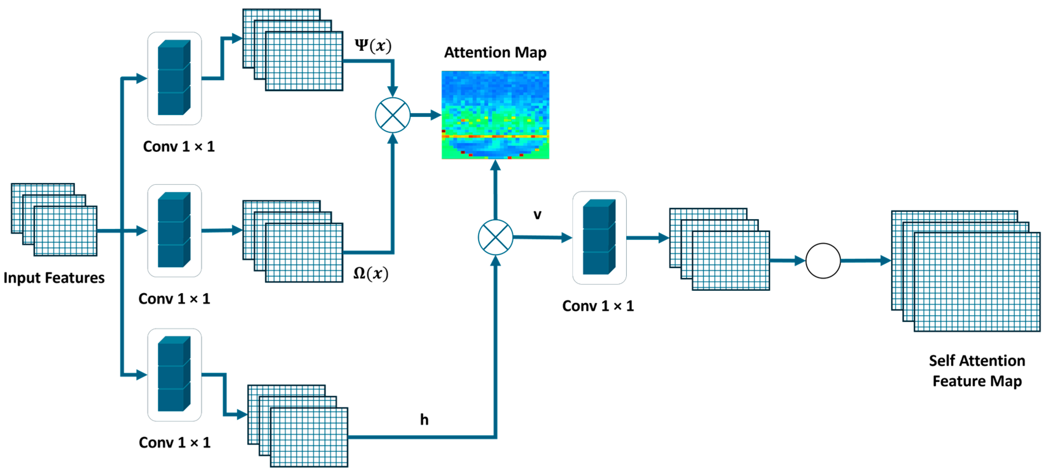
In the proposed method, a self-attention mechanism is integrated into the ResNet-50 backbone to enhance feature extraction from scalograms. Traditional CNNs primarily focus on local spatial patterns, limiting their ability to capture long-range dependencies. Self-attention mechanisms address this limitation by assigning different importance levels to different regions of the input feature maps, allowing the model to focus on the most relevant patterns for fault classification [49], as shown in Figure 4.

Figure 4. Self-attention module for feature refinement in fault classification.

SA computes relationships between all spatial locations within a feature map, forming a weighted representation that emphasizes significant regions while suppressing less informative ones. Given an input feature map $X$, the self-attention mechanism generates three transformed versions: the query $Q$, key $K$, and value $V$, computed as

$$Q=W_{q}X,K=W_{k}X,V=W_{v}X$$

(3)

where in Equation (3), $W_q$, $W_k$, $W_v$ are learnable weight matrices. The attention scores are obtained by computing the scaled dot-product similarity between $Q$ and $K$.Where in Equation (4), $d_k$ is the dimensionality of the key vectors, while the final attention output is computed by Equation (5):

$$A=softmax\left({\displaystyle \frac{Q{K}^T}{\sqrt{d_k}}}\right)$$

(4)

$$Z=AV$$

(5)

By incorporating self-attention, the network effectively captures global contextual information, improving feature discrimination in scalograms. This is particularly beneficial for fault diagnosis, where signal patterns exhibit complex variations across time and frequency. The integration of self-attention enhances the ability of the model to highlight discriminative regions, improving class separation in the feature space. In the proposed method, SA-ResNet50, SA is applied at multiple layers to refine feature representations progressively. This enables the model to focus on small differences. The ability to adaptively weigh feature importance makes self-attention particularly effective in FSL, where limited support samples require efficient feature extraction to generalize well to new queries. The overall architecture of the proposed SA-Resnet50 is provided in Table 2.

Table 2. Network Architecture of the Proposed SA-Resnet50.

Stage	Layer/Block	Output Size
Input	CWT Scalogram	224 × 224 × 3
Conv1	7 × 7 Conv, 64 filters, stride 2 + MaxPool	112 × 112 × 64
ResNet Stage 1	[1 × 1 Conv, 64] + [3 × 3 Conv, 64] × 3	56 × 56 × 256
ResNet Stage 2	[1 × 1 Conv, 128] + [3 × 3 Conv, 128] × 4	28 × 28 × 512
ResNet Stage 3	[1 × 1 Conv, 256] + [3 × 3 Conv, 256] × 6	14 × 14 × 1024
ResNet Stage 4	[1 × 1 Conv, 512] + [3 × 3 Conv, 512] × 3	7 × 7 × 2048
Attention Module	Spatial + Channel Self-Attention	7 × 7 × 2048
Global Pooling	Average Pooling	1 × 1 × 204
Embedding Layer	Fully Connected	1 × 512
Prototype Computation	APL	1 × 512
Similarity Measure	Mahalanobis Distance	Scalar
Loss Function	Contrastive Loss + Cross-Entropy	-

3.5. Adaptive Prototype Learning

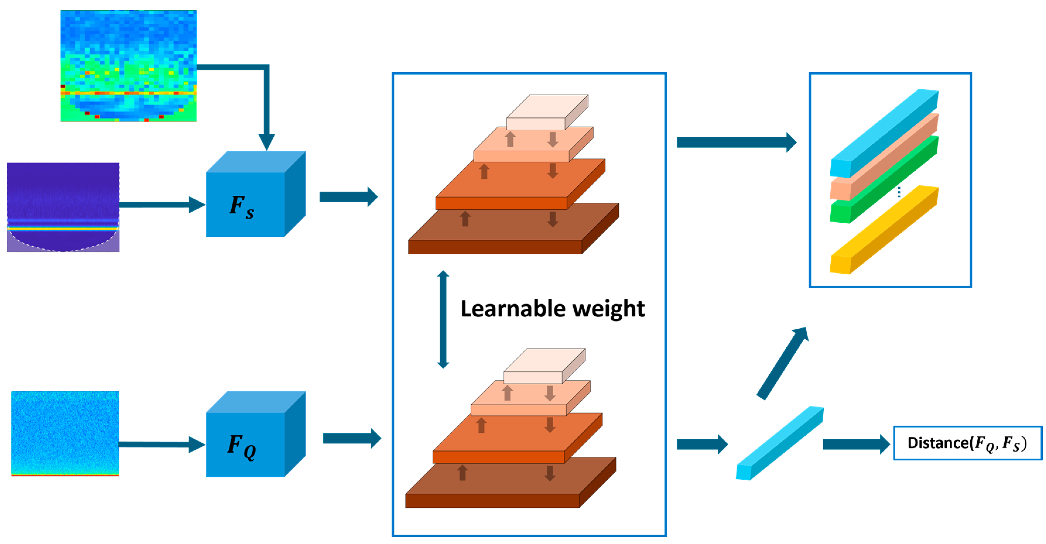
Prototype-based learning is a widely used approach in FSL, where a classifier assigns labels to query samples based on their similarity to class prototypes. A prototype is a representative feature vector computed from the support set of each class. Conventional prototypical networks compute these prototypes as the mean of all support samples belonging to a given class [40]. However, this simple averaging approach may not always capture the most informative class representations, especially in cases of high intra-class variability or noisy samples. To address this limitation, Adaptive Prototype Learning (APL) is introduced in this method as shown in Figure 5.

Figure 5. APL framework, where learnable weights adjust the support samples to generate more representative class prototypes.

APL assigns learnable importance weights to support samples, ensuring that more relevant samples contribute more to prototype computation [50]. Given a set of support embeddings $S=\{s_1,s_2,\dots ,s_N\}$ for a class $c$, the traditional prototype computation is given by

$${\mu }_c={\displaystyle \frac{1}{N}}{\sum }_{i=1}^N{s}_i$$

(6)

where in Equation (6), ${\mu }_c$ is the prototype of the class $c$ and $N$ is the number of support samples. In APL, a learnable weight vector $\omega =\{{\omega }_1, {\omega }_2, \dots ,{\omega }_N\}$ is introduced by Equation (7), where each weight determines the contribution of a specific support sample to the prototype:

$${\mu }_c= {\displaystyle \frac{1}{N}}{\sum }_{i=1}^N{\omega }_i{s}_i, where {\sum }_{i=1}^N{\omega }_i=1$$

(7)

These weights are learned during training, allowing the model to emphasize discriminative support samples while reducing the influence of less informative ones. This adaptive weighting leads to better generalization, as the prototypes dynamically adjust based on the most relevant class representations. The benefits of APL in FSL are significant. By assigning adaptive weights, the computed prototypes become more representative of class distributions, improving prototype robustness. It effectively reduces the influence of noisy or misrepresentative support samples, ensuring better handling of noisy data. Additionally, by dynamically refining prototypes based on the most relevant features, it enhances generalization. This adaptability makes APL particularly effective in fault diagnosis operating conditions where data availability is limited, ensuring more accurate and reliable predictions.

3.6. Mahalanobis Distance

Mahalanobis distance is a powerful metric that accounts for feature correlations and varying data distributions, making it well-suited for prototype-based classification. It considers the covariance structure of the feature space, allowing for more discriminative comparisons between query samples and class prototypes [45,51]. In the current work, the Mahalanobis distance is employed to measure the similarity between query embeddings and adaptive prototypes as depicted in Figure 6. This approach ensures that feature variations are considered appropriately, reducing the influence of redundant or less relevant dimensions. Given a query feature vector $x$ and a class prototype $\mu$, the Mahalanobis distance is defined by

$$D_M\left(x,\mu \right)=\sqrt{{\left(x-\mu \right)}^T{S}^{-1}(x-\mu )}$$

(8)

where in Equation (8), $S$ is the covariance matrix of the support set features. The covariance matrix is regularized using a pseudo-inverse to prevent instability when the support set is small. By incorporating the Mahalanobis distance, the proposed method improves class separation, ensuring more reliable classification of fault conditions in milling machines.

Figure 6. Query samples are matched to class prototypes using covariance-aware similarity for improved class separation.

4. Experimental Setup for Fault Diagnosis in Milling Cutting Tools

4.1. Introduction to the Experimental Setup

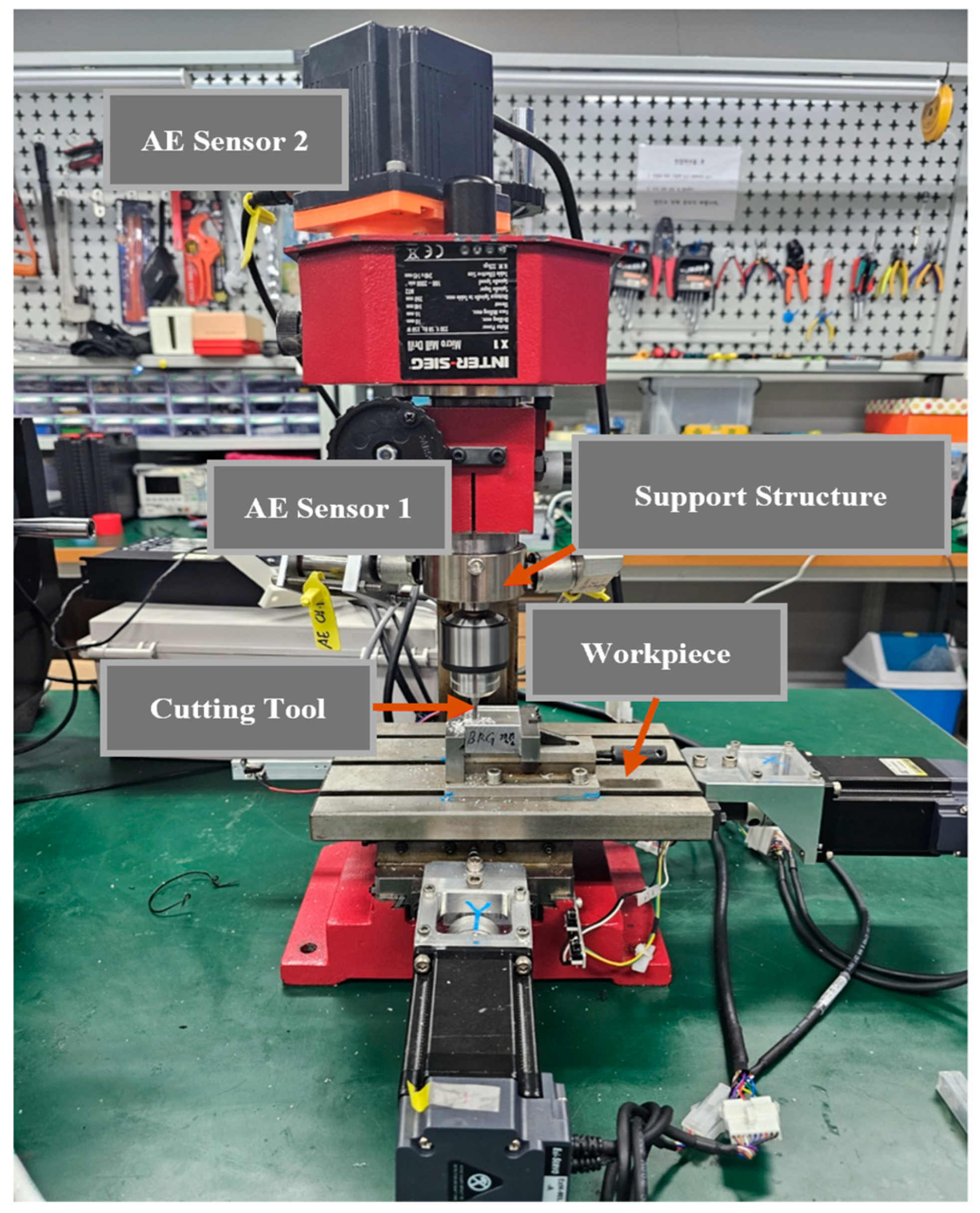
A controlled experimental setup was designed to study fault diagnosis in milling cutting tools using AE signals. This setup aimed to capture and analyze the distinct AE patterns generated during milling operations under different fault conditions. The experiment was performed on an INTER-SIEG X1 Micro Mill Drill (INTER-SIEG, Bremen, Germany), a compact milling machine constructed from cast iron, as shown in Figure 7.

Figure 7. Experimental setup of a milling machine.

This material composition provided better stability and reduced unwanted vibrations during the machining process, ensuring that only relevant AE signals were captured. The INTER-SIEG X1 Micro Mill Drill was selected for this study due to its precision in performing micro-milling tasks and its ability to simulate real-world machining conditions. The primary machining operation employed in this study was straight parallel milling, a widely used technique for shaping and cutting hard materials with high precision. This process was conducted on steel workpieces, which were chosen due to their durability and wide industrial applicability. The workpieces used in the milling process were prepared to standardized dimensions of 20 mm × 35 mm × 35 mm, ensuring uniform material interaction and consistent cutting forces throughout the experiment, as shown in Figure 8. These dimensions were carefully selected to provide a balanced contact area between the cutting tool and the workpiece, reducing variability in signal generation. The cutting depth was fixed at 2 mm to ensure stable material removal and consistent AE generation across all experiments. The machining operations were performed under strictly controlled conditions, maintaining precise control over all cutting parameters to ensure repeatability and accurate data collection. The machining operations were performed under strictly controlled conditions, maintaining precise control over all cutting parameters to ensure repeatability and accurate data collection. The cutting tool used in the milling operation was a two-flute carbide end mill, which was deliberately subjected to controlled wear. The tool was worn to an average flank wear of 0.3 mm, following the ISO-8688-2 standard, which defines the allowable wear limits before tool replacement. The intentional wear of the tool was an essential aspect of this study, as tool degradation directly affects machining performance and alters the characteristics of AE signals. By examining the AE signal variations corresponding to tool wear, it is possible to extract meaningful features indicative of cutting tool degradation.

Figure 8. Workpieces used in milling experiments: (a) unprocessed samples and (b) processed workpiece after machining.

To further ensure consistency in the machining process, the rotational speed of the motor was maintained at 1320 revolutions per minute, which corresponds to an operating frequency of 22 Hz. The spindle was rotated at 660 RPM, translating to 11 Hz. These parameters were selected based on standard milling practices, ensuring that the forces acting on the cutting tool and workpiece remained stable throughout the operation. Additionally, the bed feed rate was set to 0.4 mm per second, which allowed for controlled and uniform material removal. This slow and steady feed rate ensured that the cutting process was stable and prevented excessive tool vibration, which could introduce unwanted noise into the AE signals. The overall parameters of the experiment are mentioned in Table 3.

Table 3. Experimental Setup and Operating Conditions.

Parameters	Specifications
Milling Machine	INTER-SIEG X1 Micro Mill Drill
Spindle Rotation	660 RPM ($\approx$11 Hz)
Motor Rotation	1320 RPM ($\approx$22 Hz)
Cutting depth	2 mm
Rate Bed Feed	0.4 mm/s (under cutting conditions)
Sensors Used	Motor: 100 mV/g, Chuck: 500 mV/g
Workpiece Size	20 mm × 35 mm × 35 mm
Operating Modes	Idle state and material cutting
Fault Categories	Tool Fault (1–2 mm blade breakage), Bearing Fault (3 mm depth), Gear Fault (2–3 mm depth, 1.5 mm width)

4.2. Acoustic Emission Sensor Deployment and Data Collection System

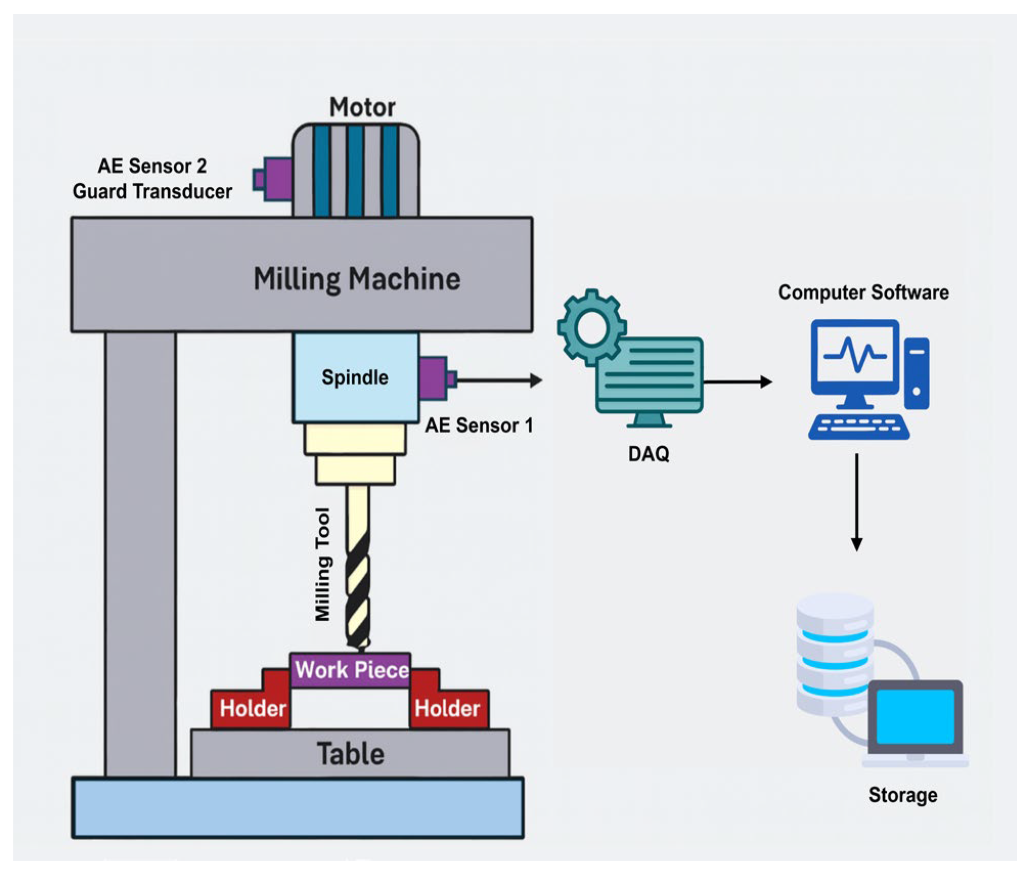
AE signals were recorded using two highly sensitive AE sensors (model R15I-AST, MISTRAS Inc., Princeton Junction, NJ, USA), which were strategically placed on the milling machine to capture transient stress waves generated during cutting and fault occurrences. The primary AE sensor was mounted on the spindle, allowing it to capture signals associated with tool wear, bearing conditions, and gear interactions. Since the spindle is directly involved in the machining process, this sensor placement ensured that all AE bursts generated by the cutting tool were recorded with high precision. The secondary AE sensor was affixed to the motor housing, acting as a guard transducer. This secondary sensor plays an important role in detecting non-relevant background noise and vibrations coming from the machine frame and motor, ensuring that the primary sensor focuses on capturing fault-related AE signatures. To achieve a strong and stable connection, both AE sensors were attached using industrial-grade adhesives, which provided a secure bond and prevented sensor displacement during high-speed operations. The sensor attachments were tested using an HSU-Nelson test, a standardized validation technique used to assess the sensitivity and performance of AE transducers. This test involved generating artificial AE bursts to ensure that both sensors were functioning correctly and capable of detecting transient acoustic signals with high accuracy.

Before initiating the cutting experiments, both AE sensors were calibrated in accordance with ASTM E976 using the Hsu–Nielsen pencil-lead break technique to ensure accurate and repeatable measurements. The calibration was performed by breaking a 0.5 mm 2H pencil lead (2–3 mm length) at multiple positions on the spindle and motor housing to generate controlled AE events. Each sensor’s sensitivity and timing were verified under identical preamplifier and filter settings (40 dB gain, 50–800 kHz band). The system noise floor was approximately 0.01 V RMS, with a detection threshold of 0.35 V (7% FS), while the average calibration peak voltage measured at the ADC input was 2.2 V (44% FS). The percentage of full scale was calculated using

$$\% FS={\displaystyle \frac{V_{peak}}{V_{FS}}}\times 100$$

(9)

where in Equation (9), $V_{FS}$ = 5 V for the NI-9223 acquisition module. These results confirmed that all AE signals remained within the linear response range of the digitizer. Furthermore, inter-channel synchronization accuracy was within ±2 µs, confirming high repeatability and proper timing alignment between sensors.

The AE signals were acquired using a National Instruments NI-9223 data acquisition system (National Instruments, Austin, TX, USA), which was selected due to its high sampling rate and precision. The sampling frequency was set to 1 MHz based on the spectral characteristics of AE signals and the operating bandwidth of the MISTRAS R15I-AST sensors (50–400 kHz). In milling operations, transient AE bursts produced during tool-workpiece interaction, wear progression, and fracture propagation typically contain frequency components extending up to approximately 450 kHz. According to the Nyquist sampling theorem, the minimum required rate for accurate signal reconstruction should be at least twice the highest signal frequency. Therefore, a 1 MHz sampling rate was chosen to ensure complete capture of all relevant fault-induced acoustic activity while avoiding aliasing. This selection also provides sufficient oversampling for precise transient analysis and reliable feature extraction. Preliminary tests at lower sampling frequencies (500–750 kHz) resulted in partial loss of high-frequency detail and minor amplitude distortion, whereas higher rates offered no additional diagnostic advantage but increased data size and computational cost. Consequently, the 1 MHz rate represents an optimal balance between signal fidelity, data efficiency, and diagnostic performance [52]. A bandpass filter was applied to the recorded AE signals to isolate the frequency components relevant to cutting-tool fault dynamics. The cutoff frequencies were determined based on both the operating bandwidth of the R15I-AST AE sensors and the observed spectral distribution of the acquired data. The sensors exhibit maximum sensitivity in the 50–400 kHz range, which encompasses the dominant energy of AE bursts produced by tool wear, bearing impacts, and gear defects. Frequencies below 50 kHz were largely attributed to mechanical vibrations of the machine frame and spindle, while frequencies above 450 kHz contained random electromagnetic interference. Accordingly, a 50–450 kHz bandpass filter was adopted to retain all relevant acoustic emission activity while suppressing low-frequency structural noise and high-frequency disturbances. This range provides an optimal balance between noise reduction and information preservation, ensuring that only fault-related AE signatures were used for feature extraction and model training. By isolating the relevant AE frequency range, the recorded data was optimized for fault diagnosis. To facilitate multi-sensor data synchronization, the data acquisition system was operated in dual-channel mode, ensuring that AE signals from both the spindle-mounted and motor-mounted sensors were recorded simultaneously. This synchronized data collection allowed for comparative analysis between normal and faulty operating conditions, making it possible to differentiate between tool-related faults and background noise. The overall setup for the AE data acquisition is shown in Figure 9.

Figure 9. Schematic diagram of the milling machine experimental setup.

4.3. Fault Introduction and Simulated Defect Conditions

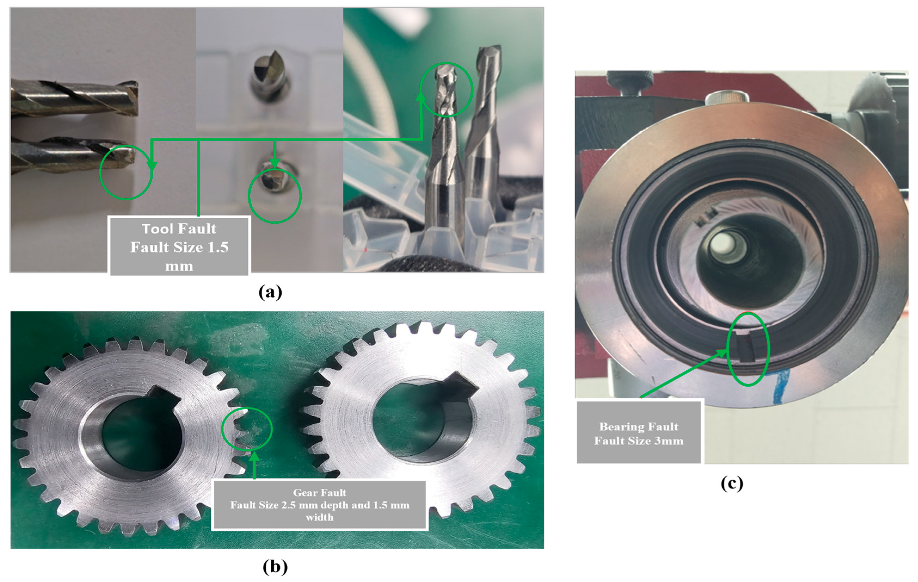
To evaluate the fault diagnosis system, three types of defects were deliberately introduced into the milling machine components. These faults were designed to mimic real-world wear and failure mechanisms commonly observed in industrial machining environments. The first fault type was tool wear, which was introduced by subjecting the cutting tool to progressive flank wear until it reached an average of 0.3 mm, as shown in Figure 10a. As the tool deteriorated, the AE signals exhibited distinct changes in energy levels, burst frequencies, and transient peak amplitudes, reflecting the increased resistance experienced during machining. The second fault involved bearing defects, which were artificially created by introducing localized damage to the outer race of the bearing, as shown in Figure 10b. This defect was designed to simulate rolling element fatigue, a common issue in high-speed machining. When the bearing defect interacted with the rotating spindle, it produced repetitive impact forces, generating periodic bursts in the AE signal. These bursts were characterized by high-amplitude oscillations and increased energy levels, making them distinguishable from normal bearing operation. The third fault concerned gear damage, introduced by removing a small metal fragment from one of the gear teeth responsible for torque transmission. The defect was created in the main spindle gearbox, which transfers torque from the motor to the spindle. A fragment approximately 2–3 mm deep and 1.5 mm wide was removed from a single gear tooth to simulate localized wear. Although this modification produced measurable AE variations, it represents a secondary diagnostic condition compared to the tool and bearing faults emphasized in this study, as shown in Figure 10c. This fault altered the load distribution in the gear system, leading to intermittent fluctuations in torque and creating irregular shock waves. These gear-related AE signals exhibited unique patterns that differentiated them from tool wear and bearing faults. All fault conditions were tested under both idle and cutting conditions, ensuring that the dataset captured AE variations across multiple operating scenarios. By recording AE signals in these conditions, it became possible to construct a robust classification model capable of distinguishing between normal operation and faulty conditions. The faults introduced in this study were designed to emulate realistic deterioration levels typically encountered in industrial milling operations rather than artificially exaggerated damage. The tool fault was produced by progressive edge wear up to an average flank wear of 0.3 mm, in compliance with ISO 8688-2 standards for allowable wear prior to tool replacement. The bearing defect involved a 3 mm localized outer race indentation, simulating rolling element fatigue and replicating natural pitting effects observed in high-speed spindles. The gear fault was introduced by removing a 2–3 mm section (1.5 mm width) from one gear tooth to create a mild imbalance in load transmission without disrupting mechanical alignment. These controlled defect magnitudes represent early to moderate fault stages that generate measurable yet non-trivial acoustic emission variations. All faults were tested under both idle and cutting conditions to capture AE signatures across varying load conditions. The resulting signals exhibited gradual changes in energy and frequency distribution, confirming that the proposed framework effectively recognizes both minor and advanced fault states. This demonstrates the system’s high sensitivity and practical applicability for early fault detection and predictive maintenance in real milling environments.

Figure 10. Faulty machine components considered in this study: (a) end-mill tool with edge damage, (b) gear with surface defect, and (c) bearing with localized fault.

4.4. Dataset Composition and Validation

For each operating condition, including normal, tool wear, bearing fault, and gear fault, a total of 280 AE signal samples were recorded. Each sample was recorded for a duration of 1 s, resulting in 1 million data points per sample due to the 1 MHz sampling rate, as shown in Table 4. The collected dataset provided a comprehensive representation of AE patterns, ensuring that the classification models could be trained with diverse signal variations.

Table 4. Data Acquisition Under Different Operating Conditions.

Operational Conditions	Samples Collected	Acquisition Rate	Duration
Normal (N)	40	1 MHz	2 min
Normal—Idle (NI)	40	1 MHz	2 min
Bearing Fault (BF)	40	1 MHz	2 min
Bearing Fault—Idle (BFI)	40	1 MHz	2 min
Gear Fault (GF)	40	1 MHz	2 min
Gear Fault—Idle (GFI)	40	1 MHz	2 min
Tool Fault (TF)	40	1 MHz	2 min

To validate the dataset, both time-domain and frequency-domain analyses were conducted. The time-domain analysis focused on measuring burst amplitude, signal energy, and transient wave patterns, as shown in Figure 11, while the frequency-domain analysis examined the spectral distribution of AE signals, detecting frequency shifts caused by different fault conditions. Additional post-processing techniques such as signal normalization, noise suppression, and feature extraction were applied to refine the dataset, improving its suitability for machine learning applications.

Figure 11. AE signals in the time domain under various operating conditions: (a) N; (b) NI; (c) BF; (d) BFI; (e) GF; (f) GFI; and (g) TF.

Synchronization of AE signals across both sensors ensured accurate comparisons between normal and faulty states, enhancing the diagnostic capability of fault classification models. The resulting dataset served as a foundation for developing advanced deep learning-based approaches for automated fault detection and predictive maintenance in milling operations. The experimental setup established in this study provides a highly controlled and repeatable framework for investigating AE-based fault diagnosis in milling cutting tools. By integrating precision machining, high-resolution AE sensing, synchronized data acquisition, and systematic fault introduction, the collected dataset is well-structured for developing intelligent fault detection models. The comprehensive data collection process ensures that real-world faults can be accurately identified, classified, and predicted, contributing to improved reliability in manufacturing operations.

5. Results

This section presents a detailed experimental evaluation of the proposed FSL framework for fault diagnosis in milling machines. The experiments were designed to replicate challenging real-world scenarios where only a limited number of labeled samples are available per fault category. All evaluations were conducted using CWT scalogram images generated from AE signals. To ensure fairness and reproducibility, the same preprocessing pipeline, training strategy, and computational environment were applied to both the proposed model and all comparison architectures. The analysis is structured into three parts: (a) overall classification performance, (b) few-shot generalization, and (c) visualization of learned representations.

The proposed approach was compared against widely used CNN architectures, including ResNet-18, ResNet-50, ShuffleNetV2, MobileNetV3 Large, DenseNet-201, and SqueezeNet. All models were trained using the same preprocessing strategy: images were resized to 224 × 224, normalized to [−1, 1], and augmented using random horizontal flips and slight rotations. Training and evaluation were conducted on a single NVIDIA RTX 3060 GPU using PyTorch 2.8.0. Classification performance was evaluated using accuracy, precision, recall, F1-score, specificity, Matthew’s correlation coefficient (MCC), and training time, as provided in Table 5. The proposed model achieved 99.32% accuracy, reflecting perfect generalization and better classification performance under data-constrained conditions. In contrast, ResNet-18 achieved 91.43% accuracy, ResNet-50 85.71%, ShuffleNetV2 70.00%, MobileNetV3 84.29%, DenseNet-201 89.29, and SqueezeNet 78.57%. Despite DenseNet-201 requiring over 11 min for training, it still underperformed compared to the proposed lightweight framework, which required only one minute. This highlights the proposed method’s better classification performance and computational efficiency, making it suitable for real-time and resource-limited industrial environments. The high precision and recall values achieved by the proposed framework demonstrate its ability to correctly classify fault conditions while minimizing both false positives and false negatives. These results confirm the model’s strong regularization ability and effective optimization under low-data conditions, with no signs of overfitting. The visual evidence aligns with these quantitative results.

Table 5. Classification Performance Comparison.

Model	Acc (%)	Prec (%)	Rec (%)	F1 (%)	MCC (%)	Spec (%)	Time (min)
ResNet-18	91.43	91.20	91.40	91.30	90.34	93.10	1:09
ResNet-50	87.14	87.00	87.10	87.00	83.57	92.00	1:15
ShuffleNetV2	70.00	73.80	70.00	71.20	58.84	88.30	0:27
MobileNetV3	84.29	84.60	84.30	84.20	80.38	91.00	0:30
DenseNet-201	89.29	89.40	89.30	89.20	80.77	93.40	11:21
SqueezeNet	78.57	78.90	78.60	78.50	71.02	90.10	1:10
Proposed	99.32	99.30	99.40	99.30	98.90	99.40	1:00

This reliability is further illustrated by the confusion matrix, which shows perfect classification across all operating conditions as shown in Figure 12a. The training curves of the proposed method further support these findings. The model exhibited a smooth ascent in accuracy and a consistent decline in loss, converging to 100% accuracy with near-zero training loss over 500 epochs, as shown in Figure 12b,c. Occasional small fluctuations in the loss were attributed to the dynamics of contrastive loss and the episodic sampling strategy, but did not impact convergence stability.

Figure 12. Result visualization of proposed method: (a) Confusion matrix, (b) Accuracy curve, (c) Loss curve, (d) t-SNE, and (e) ROC curve.

To better understand the distribution and discriminability of the learned features, we plotted t-distributed Stochastic Neighbor Embedding (t-SNE) to visualize high-dimensional embeddings in a two-dimensional space. The resulting plots showed tight intra-class clusters and well-separated inter-class margins as shown in Figure 12d, indicating the model’s capability to learn highly discriminative feature representations. This improvement can be attributed to the self-attention mechanism, which allows the model to focus on the most informative time–frequency regions in the scalograms, and the contrastive loss function, which reinforces both intra-class compactness and inter-class separation. These insights are supported by the better feature learning capacity of the model’s SA-ResNet50 backbone, which enhances the extraction of meaningful and contextually rich representations.

To further quantify the model’s decision confidence and class discrimination, Receiver Operating Characteristic (ROC) curves were plotted for each class as shown in Figure 12e. The proposed framework achieved AUC scores close to 1.0 across all fault categories, confirming its high confidence and robustness even in low-data scenarios. These high AUC values validate that the model not only distinguishes between classes with great accuracy but also maintains strong generalization across unseen query samples.

One of the core challenges in industrial fault diagnosis is adapting to conditions with extremely limited labeled samples. Table 6 presents the classification performance under 1-shot, 3-shot, and 5-shot learning setups. As expected, performance improves steadily with more labeled samples. The 1-shot configuration yielded 87.46% accuracy, sufficient for coarse classification, while the 3-shot setting improved accuracy to 93.18%. With 5 shots, the model achieved 99.32% accuracy, highlighting its ability to generalize even under highly constrained supervision. The proposed framework consistently outperformed conventional CNNs across all evaluations. Its ability to deliver high accuracy under 5-shot settings, adverse feature clustering, and computational efficiency establishes it as a highly practical solution for fault diagnosis in modern manufacturing environments.

Table 6. Few-Shot Generalization Performance.

Setting	Acc (%)	Prec (%)	Rec (%)	F1 (%)
1-shot	87.46	87.50	87.40	87.40
3-shot	93.18	93.20	93.20	93.10
5-shot	99.32	99.30	99.40	99.30

To further assess the generalization capability of the proposed method, additional experiments were conducted using datasets collected under two distinct spindle speeds: 1440 rpm and 660 rpm. These conditions were chosen to simulate different cutting environments and evaluate the robustness of the model under variable AE characteristics. The quantitative results for both spindle speeds are summarized in Table 7. At 1440 rpm, the model achieved an average precision of 97.4%, a recall of 97.2%, and an F1-score of 97.3%, indicating reliable discrimination among tool-wear classes under high-speed conditions. At 660 rpm, all performance metrics exceeded 99.8%, demonstrating the framework’s ability to maintain nearly perfect accuracy under low-speed operation. The model achieved high and balanced classification performance for both the updated and newly collected data. The confusion matrix in Figure 13a for 660 rpm displays strong diagonal dominance, and the t-SNE visualization in Figure 13b shows clear separation between all states, indicating that the learned embeddings remain discriminative under high-speed operation. The confusion matrix, as in Figure 14a for the 1440 rpm, confirms better predictions, and the t-SNE projection in Figure 14b demonstrates complete separability among the feature clusters. The model achieved high and balanced classification performance for both the updated and newly collected data. The confusion matrix in Figure 13a for 660 rpm displays strong diagonal dominance, and the t-SNE visualization shows clear separation between all states, indicating that the learned embeddings remain discriminative under high-speed operation. The confusion matrix, as in Figure 14a for the 1440 rpm, confirms better predictions, and the t-SNE projection in Figure 14b demonstrates complete separability among the feature clusters. These results clearly indicate that the proposed framework maintains consistent discriminative ability across different spindle speeds. The consistent results across both speed operations validate the robustness and stability of the proposed network and confirm its ability to generalize effectively across diverse machining conditions.

Table 7. Comparative Performance of the Proposed Model Under Different Spindle Speeds.

Spindle Speed (rpm)	Class	Precision	Recall	F1-Score	Support
660	BF	0.998	0.999	0.998	15
	GF	0.999	0.997	0.998	15
	N	0.998	0.998	0.998	15
	TF	0.999	0.999	0.999	15
	Macro Avg	0.999	0.998	0.998	60
1440	BF	0.976	0.973	0.974	14
	GF	0.972	0.974	0.973	14
	N	0.974	0.970	0.972	14
	TF	0.975	0.972	0.974	14
	Macro Avg	0.974	0.972	0.973	56

Figure 13. Results for the 660 rpm dataset: (a) confusion matrix, and (b) t-SNE visualization.

Figure 14. Results for the 1440 rpm dataset: (a) confusion matrix, and (b) t-SNE visualization.

6. Discussion

The integration of Mahalanobis distance into the prototype matching process played a significant role in enhancing classification robustness. Unlike other distances, Mahalanobis distance considers the covariance structure of class-wise features, allowing for more accurate similarity matching, especially in cases involving subtle signal differences. Furthermore, the adaptive prototype learning mechanism dynamically refined class representations during training, improving intra-class consistency and inter-class distinctiveness. These components, working together with contrastive loss, contributed to robust class separability and minimized misclassifications. The proposed model’s strong few-shot learning performance is thus attributed to this combination of adaptive prototype learning, attention-guided representation, and covariance-aware matching, which enables it to generalize effectively even under data scarcity.

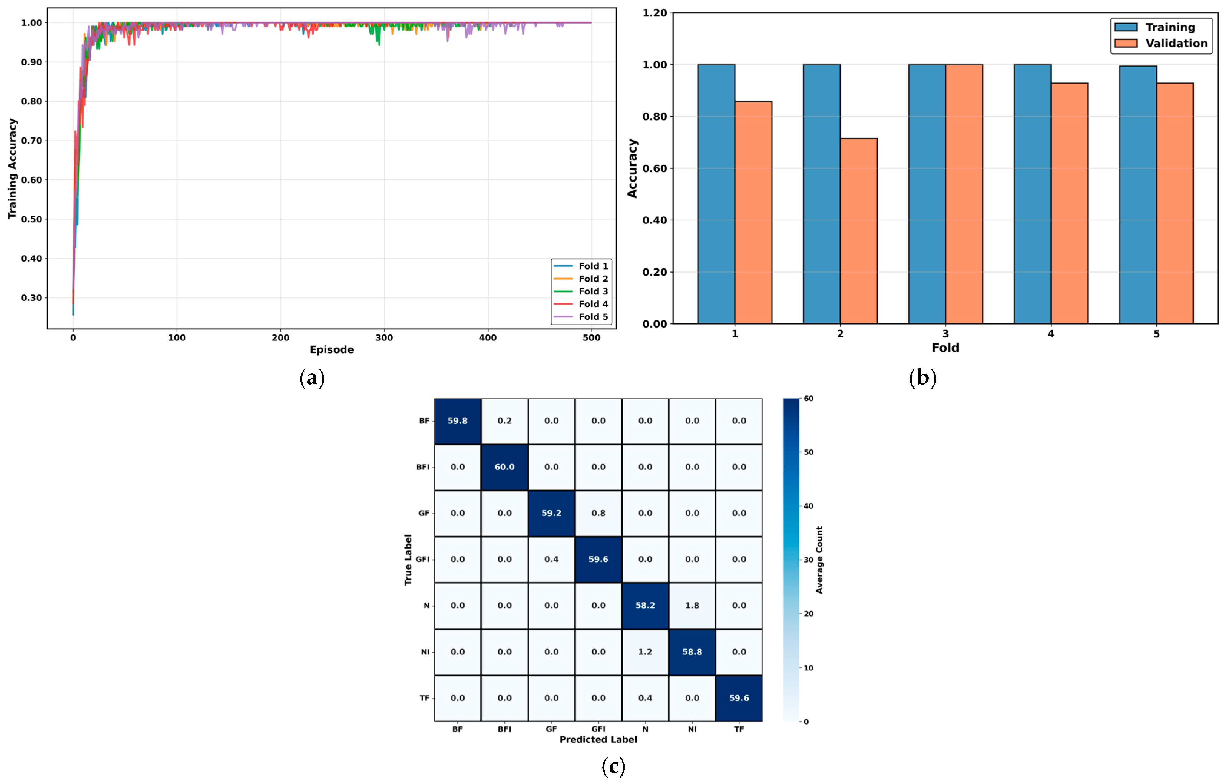
To address concerns regarding overfitting in the proposed method, a comprehensive 5-fold stratified cross-validation was conducted to rigorously evaluate the robustness and generalization. The detailed fold-wise results confirm that the model maintains better consistency across all partitions, with validation accuracy ranging from 97.14% to 100% and a mean accuracy of 98.86% ± 0.97% (95% CI = [98.01%, 99.71%]). The low standard deviation (σ = 0.97%) across folds indicates that the model’s performance is not sensitive to specific train-test splits. The training dynamics illustrated in Figure 15 a show uniform and stable convergence behavior across all five folds, with each fold achieving rapid convergence within the first 200 episodes. The training-validation comparison shown in Figure 15b further supports this, as the performance gap remains consistently narrow (≈1% on average) between the training accuracy (99.99% ± 0.02%) and validation accuracy (98.86% ± 0.97%). Such a minimal gap demonstrates effective generalization and indicates that the model learns meaningful prototypical representations. Moreover, the mean confusion matrix in Figure 15c exhibits pronounced diagonal dominance across all seven conditions, underscoring the model’s discriminative ability and class-level stability. The strong consistency across folds substantiates that the proposed network achieves reliable few-shot learning performance even under constrained data conditions. Although environmental noise and sensor calibration can affect AE data acquisition, the use of the Hsu–Nielsen test and 50–450 kHz band-pass filtering ensured consistent sensor sensitivity and minimized external interference during all experiments.

Figure 15. 5-fold cross-validation results of the proposed model: (a) training convergence across folds, (b) training vs. validation accuracy comparison, and (c) mean confusion matrix showing consistent classification performance.

To further interpret the network’s decision process, Gradient-weighted Class Activation Mapping++ (Grad-CAM++) was applied to visualize the most influential regions within the CWT scalograms. Figure 16 presents the class-wise average activation maps for all seven fault conditions (BF, BFI, GF, GFI, N, NI, and TF). The red regions indicate higher activation intensity, representing the areas where the model focused during classification. The visualization results show that each fault type activates distinct time–frequency regions, revealing the network’s ability to capture fault-specific acoustic characteristics. For example, severe breakage conditions (BF, TF) show concentrated activations in high-frequency regions associated with impact-type emissions, whereas gradual wear faults (GF, GFI) produce distributed mid-frequency responses. The normal states (N, NI) exhibit low and stable activation areas, corresponding to the absence of sudden AE bursts. These findings confirm that the attention-augmented ResNet backbone effectively emphasizes meaningful discriminative patterns rather than noise. Overall, the Grad-CAM++ analysis provides valuable interpretability by visualizing the relationship between learned representations and physical fault behaviors, thereby reinforcing the transparency and reliability of the proposed few-shot learning framework for fault diagnosis.

Figure 16. Class-wise Grad-CAM++ activation maps showing discriminative time–frequency regions.

These findings confirm the proposed framework’s effectiveness in overcoming the core challenges of few-shot fault diagnosis in milling machine applications. Its perfect classification performance, interpretability through visualization tools, strong generalization under minimal data, and computational efficiency establish it as a strong candidate for real-world deployment. The framework is highly scalable and adaptable, and through its integration of adaptive prototype learning, Mahalanobis distance, and attention-driven feature extraction, consistently outperforms baseline few-shot learning approaches. It holds strong potential for extension to other industrial domains such as predictive maintenance, real-time monitoring, and anomaly detection. In summary, the proposed framework consistently demonstrated near-perfect performance under the 5-shot settings while maintaining strong generalization under more restrictive conditions. Its scalability, interpretability, and computational efficiency make it a practical and robust solution for real-world milling machine fault diagnosis.

Although the proposed framework demonstrates strong diagnostic performance and robustness across varying spindle speeds, certain limitations remain that present valuable opportunities for future improvement. The present study was conducted using AE data collected under controlled laboratory conditions, which may not fully capture the range of variability present in real industrial environments. Future work will therefore focus on extending the dataset to include multiple machines, tool materials, and cutting parameters to further validate domain generalization. In addition, while the current model performs effectively in offline analysis, deploying it in real-time monitoring systems will require optimization for computational efficiency and latency reduction. Moreover, since this study relied solely on AE signals, future extensions will explore the integration of multi-sensor information, such as vibration, cutting force, and spindle current, to improve robustness under noisy conditions. Finally, further evaluation under extremely low-shot or cross-domain conditions will be pursued to enhance model stability and adaptability. Addressing these aspects will help transition the proposed framework from laboratory validation to a fully scalable and explainable deployment in industrial TCM.

7. Conclusions

This paper presented an optimized Few-Shot Learning framework for fault diagnosis in milling machines using acoustic emission (AE) signals. The approach effectively addresses the challenges of data scarcity and non-stationary signal behavior by integrating CWT-based time–frequency feature extraction, self-attention ResNet-50 encoding, and adaptive prototype learning with Mahalanobis distance matching. The incorporation of contrastive loss with hard negative mining further enhances class separability, leading to compact and well-defined embedding spaces. Experimental validations conducted under multiple spindle speeds (660 rpm and 1440 rpm) and 5-fold stratified cross-validation confirm the robustness and reproducibility of the model, with consistently high accuracy, precision, and F1-scores across all partitions. The narrow performance variance (σ = 0.97%) demonstrates that the model generalizes effectively beyond specific train–test splits. Moreover, interpretability analysis using Grad-CAM++ visualizations revealed that the network attends to fault-relevant signal regions, providing transparency in the decision-making process. The findings highlight the framework’s strong diagnostic sensitivity across both minor and severe fault stages, reflecting its real-world applicability for early-stage fault detection and predictive maintenance. While the model shows outstanding performance on controlled laboratory data, its reliance on AE signals from a single machine setup represents a limitation that future work will address through multi-machine validation, domain adaptation, and multi-modal sensor integration. Future research will also explore online learning strategies and adaptive episodic training to enhance real-time deployment in dynamic industrial environments. Overall, the proposed framework provides a reliable, data-efficient, and interpretable AI solution for intelligent fault diagnosis in modern manufacturing systems.

References

1. Soori, M.; Arezoo, B.; Dastres, R. Machine learning and artificial intelligence in CNC machine tools, A review. Sustain. Manuf. Serv. Econ. 2023, 2, 100009. [Google Scholar] [CrossRef]
2. Przybyś-Małaczek, A.; Antoniuk, I.; Szymanowski, K.; Kruk, M.; Kurek, J. Application of Machine Learning Algorithms for Tool Condition Monitoring in Milling Chipboard Process. Sensors 2023, 23, 5850. [Google Scholar] [CrossRef]
3. Umar, M.; Ahmad, Z.; Ullah, S.; Saleem, F.; Siddique, M.F.; Kim, J.-M. Advanced Fault Diagnosis in Milling Machines Using Acoustic Emission and Transfer Learning. IEEE Access 2025, 13, 100776–100790. [Google Scholar] [CrossRef]
4. Zhu, Z.; Tang, X.; Chen, C.; Peng, F.; Yan, R.; Zhou, L.; Li, Z.; Wu, J. High precision and efficiency robotic milling of complex parts: Challenges, approaches and trends. Chin. J. Aeronaut. 2022, 35, 22–46. [Google Scholar] [CrossRef]
5. Wang, W.; Guo, Q.; Yang, Z.; Jiang, Y.; Xu, J. A state-of-the-art review on robotic milling of complex parts with high efficiency and precision. Robot. Comput. Integr. Manuf. 2023, 79, 102436. [Google Scholar] [CrossRef]
6. Kaliyannan, D.; Thangamuthu, M.; Pradeep, P.; Gnansekaran, S.; Rakkiyannan, J.; Pramanik, A. Tool Condition Monitoring in the Milling Process Using Deep Learning and Reinforcement Learning. J. Sens. Actuator Netw. 2024, 13, 42. [Google Scholar] [CrossRef]
7. Bourassa, D.; Gauthier, F.; Abdul-Nour, G. Equipment failures and their contribution to industrial incidents and accidents in the manufacturing industry. Int. J. Occup. Saf. Ergon. 2016, 22, 131–141. [Google Scholar] [CrossRef] [PubMed]
8. Ahmad, Z.; Ullah, S.; Maliuk, A.S.; Kim, J.-M. Milling machine fault detection and identification based on a novel vitality index and temporal-residual network. Appl. Acoust. 2025, 239, 110861. [Google Scholar] [CrossRef]
9. Cavalcante, C.A.V.; Lopes, R.S.; Scarf, A. Inspection and replacement policy with a fixed periodic schedule. Reliab. Eng. Syst. Saf. 2021, 208, 107402. [Google Scholar] [CrossRef]
10. Twardowski, P.; Tabaszewski, M.; Wiciak-Pikuła, M.; Felusiak-Czyryca, A. Identification of tool wear using acoustic emission signal and machine learning methods. Precis. Eng. 2021, 72, 738–744. [Google Scholar] [CrossRef]
11. Zhou, J.-H.; Pang, C.K.; Zhong, Z.-W.; Lewis, F.L. Tool Wear Monitoring Using Acoustic Emissions by Dominant-Feature Identification. IEEE Trans. Instrum. Meas. 2011, 60, 547–559. [Google Scholar] [CrossRef]
12. Zhou, Y.; Liu, C.; Yu, X.; Liu, B.; Quan, Y. Tool wear mechanism, monitoring and remaining useful life (RUL) technology based on big data: A review. SN Appl. Sci. 2022, 4, 232. [Google Scholar] [CrossRef]
13. Cheng, Y.; Gai, X.; Guan, R.; Jin, Y.; Lu, M.; Ding, Y. Tool wear intelligent monitoring techniques in cutting: A review. J. Mech. Sci. Technol. 2023, 37, 289–303. [Google Scholar] [CrossRef]
14. Pimenov, D.Y.; Gupta, M.K.; da Silva, L.R.R.; Kiran, M.; Khanna, N.; Krolczyk, G.M. Application of measurement systems in tool condition monitoring of Milling: A review of measurement science approach. Measurement 2022, 199, 111503. [Google Scholar] [CrossRef]
15. Dimla, D.E. Sensor signals for tool-wear monitoring in metal cutting operations—A review of methods. Int. J. Mach. Tools Manuf. 2000, 40, 1073–1098. [Google Scholar] [CrossRef]
16. Zaman, W.; Siddique, M.F.; Ullah, S.; Saleem, F.; Kim, J.-M. Hybrid Deep Learning Model for Fault Diagnosis in Centrifugal Pumps: A Comparative Study of VGG16, ResNet50, and Wavelet Coherence Analysis. Machines 2024, 12, 905. [Google Scholar] [CrossRef]
17. Sick, B. ON-LINE AND INDIRECT TOOL WEAR MONITORING IN TURNING WITH ARTIFICIAL NEURAL NETWORKS: A REVIEW OF MORE THAN A DECADE OF RESEARCH. Mech. Syst. Signal Process 2002, 16, 487–546. [Google Scholar] [CrossRef]
18. Umar, M.; Siddique, M.F.; Ullah, N.; Kim, J.-M. Milling Machine Fault Diagnosis Using Acoustic Emission and Hybrid Deep Learning with Feature Optimization. Appl. Sci. 2024, 14, 10404. [Google Scholar] [CrossRef]
19. Nasir, V.; Dibaji, S.; Alaswad, K.; Cool, J. Tool wear monitoring by ensemble learning and sensor fusion using power, sound, vibration, and AE signals. Manuf. Lett. 2021, 30, 32–38. [Google Scholar] [CrossRef]
20. Prickett, W.; Johns, C. An overview of approaches to end milling tool monitoring. Int. J. Mach. Tools Manuf. 1999, 39, 105–122. [Google Scholar] [CrossRef]
21. Marinescu, I.; Axinte, D.A. A critical analysis of effectiveness of acoustic emission signals to detect tool and workpiece malfunctions in milling operations. Int. J. Mach. Tools Manuf. 2008, 48, 1148–1160. [Google Scholar] [CrossRef]
22. Turšič, N.; Klančnik, S. Tool Condition Monitoring Using Machine Tool Spindle Current and Long Short-Term Memory Neural Network Model Analysis. Sensors 2024, 24, 2490. [Google Scholar] [CrossRef]
23. Yan, S.; Sui, L.; Wang, S.; Sun, Y. On-line tool wear monitoring under variable milling conditions based on a condition-adaptive hidden semi-Markov model (CAHSMM). Mech. Syst. Signal Process 2023, 200, 110644. [Google Scholar] [CrossRef]
24. Zhou, Y.; Zhi, G.; Chen, W.; Qian, Q.; He, D.; Sun, B.; Sun, W. A new tool wear condition monitoring method based on deep learning under small samples. Measurement 2022, 189, 110622. [Google Scholar] [CrossRef]
25. Xiang, G.; Chen, W.; Peng, Y.; Wang, Y.; Qu, C. Deep Transfer Learning Based on Convolutional Neural Networks for Intelligent Fault Diagnosis of Spacecraft. In Proceedings of the 2020 Chinese Automation Congress (CAC), Shanghai, China, 6–8 November 2020; pp. 5522–5526. [Google Scholar] [CrossRef]
26. Siddique, M.F.; Saleem, F.; Umar, M.; Kim, C.H.; Kim, J.-M. A Hybrid Deep Learning Approach for Bearing Fault Diagnosis Using Continuous Wavelet Transform and Attention-Enhanced Spatiotemporal Feature Extraction. Sensors 2025, 25, 2712. [Google Scholar] [CrossRef] [PubMed]
27. Yan, J.; Cheng, Y.; Wang, Q.; Liu, L.; Zhang, W.; Jin, B. Transformer and Graph Convolution-Based Unsupervised Detection of Machine Anomalous Sound Under Domain Shifts. IEEE Trans. Emerg. Top. Comput. Intell. 2024, 8, 2827–2842. [Google Scholar] [CrossRef]
28. Zhu, Z.; Lei, Y.; Qi, G.; Chai, Y.; Mazur, N.; An, Y.; Huang, X. A review of the application of deep learning in intelligent fault diagnosis of rotating machinery. Measurement 2023, 206, 112346. [Google Scholar] [CrossRef]
29. Saleem, F.; Ahmad, Z.; Kim, J.-M. Real-Time Pipeline Leak Detection: A Hybrid Deep Learning Approach Using Acoustic Emission Signals. Appl. Sci. 2024, 15, 185. [Google Scholar] [CrossRef]
30. Lupea, I.; Lupea, M. Continuous Wavelet Transform and CNN for Fault Detection in a Helical Gearbox. Appl. Sci. 2025, 15, 950. [Google Scholar] [CrossRef]
31. Barbosh, M.; Dunphy, K.; Sadhu, A. Acoustic emission-based damage localization using wavelet-assisted deep learning. J. Infrastruct. Preserv. Resil. 2022, 3, 6. [Google Scholar] [CrossRef]
32. Saleem, F.; Ahmad, Z.; Siddique, M.F.; Umar, M.; Kim, J.-M. Acoustic Emission-Based Pipeline Leak Detection and Size Identification Using a Customized One-Dimensional DenseNet. Sensors 2025, 25, 1112. [Google Scholar] [CrossRef] [PubMed]
33. Zhang, B.; Wang, W.; He, Y. A hybrid approach combining deep learning and signal processing for bearing fault diagnosis under imbalanced samples and multiple operating conditions. Sci. Rep. 2025, 15, 13606. [Google Scholar] [CrossRef] [PubMed]
34. Neupane, D.; Bouadjenek, M.R.; Dazeley, R.; Aryal, S. Data-driven machinery fault diagnosis: A comprehensive review. Neurocomputing 2025, 627, 129588. [Google Scholar] [CrossRef]
35. LeCun, Y.; Bengio, Y.; Hinton, G. Deep learning. Nature 2015, 521, 436–444. [Google Scholar] [CrossRef]
36. Gao, Y.; Li, H.; Fu, W. Few-shot learning for image-based bridge damage detection. Eng. Appl. Artif. Intell. 2023, 126, 107078. [Google Scholar] [CrossRef]
37. Li, K.; Ye, H.; Gao, X.; Zhang, L. Meta-Learning With Intraclass and Interclass Optimization for Few-Shot Fault Diagnosis. IEEE Trans. Industr Inform. 2025, 21, 713–722. [Google Scholar] [CrossRef]
38. Liang, X.; Zhang, M.; Feng, G.; Wang, D.; Xu, Y.; Gu, F. Few-Shot Learning Approaches for Fault Diagnosis Using Vibration Data: A Comprehensive Review. Sustainability 2023, 15, 14975. [Google Scholar] [CrossRef]
39. Wang, D.; Zhang, M.; Xu, Y.; Lu, W.; Yang, J.; Zhang, T. Metric-based meta-learning model for few-shot fault diagnosis under multiple limited data conditions. Mech. Syst. Signal Process 2021, 155, 107510. [Google Scholar] [CrossRef]
40. Li, K.; Shang, C.; Ye, H. Reweighted Regularized Prototypical Network for Few-Shot Fault Diagnosis. IEEE Trans. Neural Netw. Learn. Syst. 2024, 35, 6206–6217. [Google Scholar] [CrossRef]
41. ALataiqeh, M.; Shi, H.; Qu, Q.; Mei, X.; Wang, H. A Novel Approach to a Few Shot Learning Techniques Based on Thermal Error Modeling for Slant Bed CNC Lathe Machine. Int. J. Precis. Eng. Manuf. 2025, 26, 1431–1448. [Google Scholar] [CrossRef]
42. Gong, Z.; Huo, D. Tool condition monitoring in micro milling of brittle materials. Precis. Eng. 2024, 87, 11–22. [Google Scholar] [CrossRef]
43. Wen, L.; Li, X.; Gao, L.; Zhang, Y. A New Convolutional Neural Network-Based Data-Driven Fault Diagnosis Method. IEEE Trans. Ind. Electron. 2018, 65, 5990–5998. [Google Scholar] [CrossRef]
44. Zhao, R.; Yan, R.; Chen, Z.; Mao, K.; Wang, P.; Gao, R.X. Deep learning and its applications to machine health monitoring. Mech. Syst. Signal Process 2019, 115, 213–237. [Google Scholar] [CrossRef]
45. Vu, M.-H.; Nguyen, V.-Q.; Tran, T.-T.; Pham, V.-T.; Lo, M.-T. Few-Shot Bearing Fault Diagnosis Via Ensembling Transformer-Based Model With Mahalanobis Distance Metric Learning From Multiscale Features. IEEE Trans. Instrum. Meas. 2024, 73, 1–18. [Google Scholar] [CrossRef]
46. Chen, Y.; Yue, J.; Liu, Z.; Chen, J. A semi-supervised wise-attention weighted prototype network for rolling bearing fault diagnosis under noisy and limited labeled data conditions. Neurocomputing 2025, 647, 130563. [Google Scholar] [CrossRef]
47. Ahmed, Y.S.; Arif, A.F.M.; Veldhuis, S.C. Application of the wavelet transform to acoustic emission signals for built-up edge monitoring in stainless steel machining. Measurement 2020, 154, 107478. [Google Scholar] [CrossRef]
48. Xie, S.; Girshick, R.; Dollar, P.; Tu, Z.; He, K. Aggregated Residual Transformations for Deep Neural Networks. In Proceedings of the 2017 IEEE Conference on Computer Vision and Pattern Recognition (CVPR), Honolulu, HI, USA, 21–26 July 2017; pp. 5987–5995. [Google Scholar] [CrossRef]
49. Yu, M.; Liu, H.; Wang, R.; Kong, X.; Hu, Z.; Li, X. An improved CNN based on attention mechanism with multi-domain feature fusion for bearing fault diagnosis. In Proceedings of the 2021 IEEE International Conference on Prognostics and Health Management (ICPHM), Detroit, MI, USA, 7–9 June 2021; pp. 1–7. [Google Scholar] [CrossRef]
50. Li, X.; Li, Y.; Zheng, Y.; Zhu, R.; Ma, Z.; Xue, J.; Cao, J. ReNAP: Relation network with adaptiveprototypical learning for few-shot classification. Neurocomputing 2023, 520, 356–364. [Google Scholar] [CrossRef]
51. Zhao, X.; Zhao, Z.; Cui, X.; Yin, J.; Cao, J.; Wang, H. Few-shot Bearing Fault Diagnosis using Adaptive Detail Convolution and Global KAN-Transformer with Mahalanobis Distance. J. Vib. Eng. Technol. 2025, 13, 296. [Google Scholar] [CrossRef]
52. Magadán, L.; Ruiz-Cárcel, C.; Granda, J.C.; Suárez, F.J.; Starr, A. Explainable and interpretable bearing fault classification and diagnosis under limited data. Adv. Eng. Inform. 2024, 62, 102909. [Google Scholar] [CrossRef]
Disclaimer/Publisher’s Note: The statements, opinions and data contained in all publications are solely those of the individual author(s) and contributor(s) and not of MDPI and/or the editor(s). MDPI and/or the editor(s) disclaim responsibility for any injury to people or property resulting from any ideas, methods, instructions or products referred to in the content.
Article Metrics
Citations
Article Access Statistics
Multiple requests from the same IP address are counted as one view.