Article

A Multi-Constraint Assembly Registration Method Based on Actual Machined Surfaces

1
Department of Mechanical Engineering, Beijing Institute of Technology, No. 5 Zhongguancun South Street, Haidian District, Beijing 100081, China
2
Beijing Institute of Computer Application, No. 10 Chedaogou, Haidian District, Beijing 100089, China
*
Authors to whom correspondence should be addressed.
Machines 2025, 13(11), 1009; https://doi.org/10.3390/machines13111009
Submission received: 17 September 2025 / Revised: 23 October 2025 / Accepted: 30 October 2025 / Published: 2 November 2025
(This article belongs to the Section Advanced Manufacturing)

Abstract

Modern manufacturing places increasing demands on assembly accuracy, revealing the limitations of conventional tolerance-based methods and studies that oversimplify multi-surface constraints into single-surface problems. To address this challenge, it is crucial to account for geometric distribution errors on multiple surfaces and constraints from multiple mating surfaces, analyzing their coupling effects in assembly. This paper presents a model that incorporates the effects of machining-induced geometric distribution errors and the constraints arising from multiple mating surfaces. The model determines contact points between two pairs of mating surfaces and calculates the spatial pose of the assembled part to predict assembly accuracy. The model validation was conducted in two stages: initial verification of fundamental principles through a two-dimensional simulation, followed by experimental validation. The experimental study involved mating surfaces with distinct geometric distribution errors manufactured by different machine tools. Assembly tests were performed under two distinct orientations of applied external forces. Results show close agreement between predicted and measured values, with a root mean square error (RMSE) below 2%, confirming the method’s effectiveness. The proposed method offers a solution to the assembly registration problem involving coupled multi-constraints and geometric distribution errors.

1. Introduction

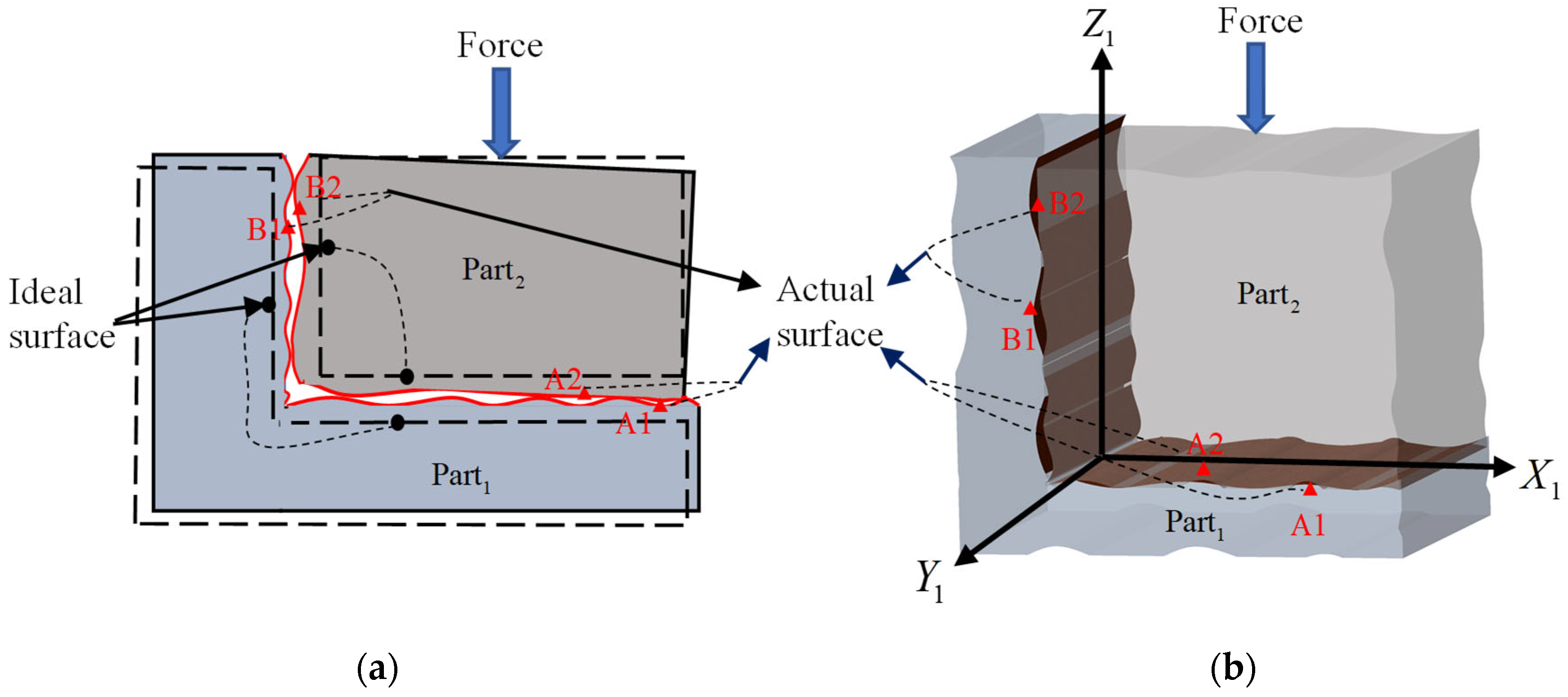
As the cornerstone of manufacturing, machine tools are crucial for processing various components. The assembly accuracy of a machine tool itself, as well as that of other key rigid components such as guideways and shafts, directly determines the precision of the final product. In assembly processes, components are often constrained by two or more mating surfaces simultaneously. Moreover, with ever-increasing demands for higher assembly precision, the impact of geometric distribution errors has become critical, especially for products characterized by these complex multi-surface constraints. Geometric distribution error refers to the deviation of a real surface from its ideal geometric form, where this deviation exhibits an inconsistent spatial distribution [1,2,3]. Figure 1 illustrates the spatial distribution of these form errors and their mechanism affecting assembly accuracy. As shown in Figure 1a, geometric distribution errors can induce angular deflection in an assembled component. Furthermore, the applied external force influences the final assembly pose (Figure 1b). This study focuses on stable assembly conditions where the force magnitude is sufficient to maintain contact stability. Moreover, the coupling effects arising from multiple mating constraints further complicate the prediction of assembly accuracy (Figure 1c).
This multi-constraint problem with geometric distribution errors is fundamentally a spatial surface-registration problem. Due to these errors, mating surfaces form discrete point contacts rather than ideal full-surface contact. Additionally, constraints between paired surfaces exhibit coupling effects: a change in one pair’s contact state alters the other pair’s state. External forces may further modify part positioning. In this study, we define this process as multi-constraint coupled surface registration, where parts progressively conform under geometric distribution errors and the applied forces until a stable contact-point set is established. Its primary objective is to address the spatial surface-registration problem by integrating the influence of geometric distribution errors, multi-constraint coupled effect, and applied external forces, thereby providing a basis toward predictive assembly pose determination.
The assembly of constrained structures with multiple mating surfaces has been widely studied. The foundational work for assembly sequence analysis was established by Mantripragada et al. [4]. Subsequent studies have traced assembly error sources and proposed error propagation models for multi-station assembly systems [5], while others have investigated the influence of locating features and datum sequences [6,7]. Further research has explored criteria for assembly positioning priority [8], developed clearance variation algorithms based on prioritizing assembly feature constraints [9], and analyzed the coupled effects of multiple error sources in complex assemblies [10]. However, most of the studies are tolerance-based, where tolerances merely describe the permissible variation range of geometric errors. thereby neglecting the spatial distributions of geometric distribution errors resulting from machining. Meanwhile, the true registration state between mating surfaces remains obscured. Furthermore, some computational methods, such as the deviation domain method [11], Jacobian-Torsor model [12,13], and point-based techniques [14,15], and iterative closest point method [16,17], also neglect the critical impact of process-induced geometric distribution errors and the contact states at the mating surfaces.
To address these gaps, recent efforts such as the method proposed by Shen et al. [18] have been made to incorporate assembly process parameters and to adopt distinct methods for different mating surface types. However, their method suffers from some limitations: its reliance on Gaussian-distributed random data, rather than on measured data from actual machined surfaces, and it does not determine contact points. These points are critical because geometric distribution errors on part surfaces cause the actual contact area to be much smaller than the nominal area, resulting in only limited points or localized contact. Ultimately, it is these discrete contact points (not the nominal surfaces) that determine the final assembly pose. Meanwhile, explorations into geometric distribution errors have been conducted, such as their effects on shaft-hole and cylindrical part assemblies using Newton-Raphson techniques [19], and systematic analyses of multifactorial impacts (including geometric distribution errors and waviness) on assembly precision [20,21,22]. Computer-aided methods have also been employed to demonstrate how machining variations affect product functionality [23], and deep learning algorithms have shown high accuracy in predicting coaxiality in aero-engine assembly by integrating geometric distribution error models [24]. Despite these valuable contributions, a key limitation persists: the predominant focus remains on single mating surfaces as assembly datums. Moreover, approaches such as differential surface methods [25], constrained registration techniques [26], and the quaternion-based method [27] overlook the critical influence of applied external forces. Furthermore, the method proposed by Samper et al. [28] may yield non-unique solutions.
To address these challenges, this study proposes a multi-constraint coupled registration method that is driven by actual measured data (geometric distribution errors) and accounts for critical assembly parameters (applied external forces). The proposed framework utilizes the NURBS method to characterize geometric distribution errors and integrates a hierarchical strategy to construct a multi-constraint coupled model. Subsequently, a penalty-function-based optimization is solved via a hybrid particle swarm algorithm. Finally, the method is validated on a two-dimensional (2D) model to verify its capability in determining both the contact points and the assembled pose, and is then extended to three-dimensional (3D) assemblies with experimental confirmation of its accuracy.

2. Multi-Constraint Coupled Registration Method

This study assumes all components as rigid bodies, neglecting deformation effects, due to the high stiffness of the parts in the target systems (e.g., machine tools). Under this assumption [29], this paper proposes a hierarchical Multi-Constraint Coupled model to resolve the multi-constraint coupling problem, providing contact points and assembly poses that better reflect actual assembly conditions. The following subsections present the details of this model.

2.1. Modeling of Coupled Multi-Constraints

To accurately characterize geometric distribution errors on part surfaces, the surface is scanned using a coordinate measuring machine (CMM) to acquire point cloud data, which is then reconstructed using non-uniform rational B-splines (NURBS) [30]. Machining errors on part surfaces consist of systematic and random components. When the machining process is consistent, the systematic error is deterministic and exhibits repeatable patterns, whereas it is this component that dominates the overall error distribution [31]. In contrast, the random error, which lacks discernible regularity, typically accounts for only a minor proportion. Accordingly, this study focuses on extracting the systematic error as the primary contributor to the assembly error model.
S a ( u , v ) = S d ( u , v ) + e r ( u , v ) S d ( u , v ) = i = 0 m j = 0 n N i , 3 ( u ) N j , 3 ( v ) P i , j
where S a ( u , v ) is the actual machined surface, u and v are the two direction parameters of the rectangular domain; S d ( u , v ) is the deterministic component of the surface that can be obtained by regression, and expressed with NURBS surface; P i , j are the control points, N i , 3 , N j , 3 are the basic functions of cubic B-spline; e r ( u , v ) are the random errors.
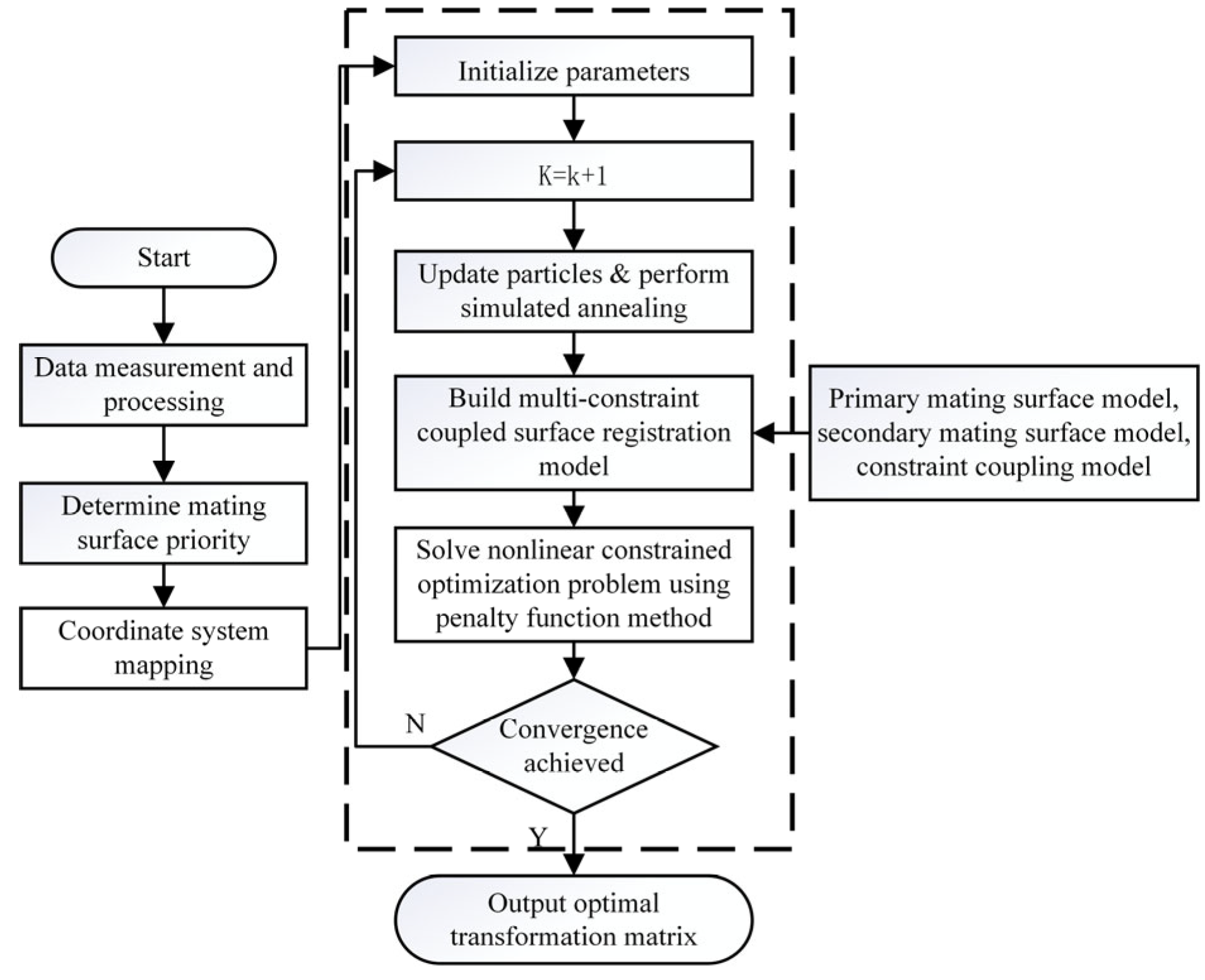
Next, we construct the multi-constraint coupled model (see flowchart in Figure 2) through the following steps. For clarity in methodology presentation, planar contact is employed due to its prevalence in machine tool structures.
Step 1: Data Measurement and Processing
This case involves plane-to-plane mating surfaces (Figure 3), comprising two pairs of mating surfaces. The point clouds of mating surfaces SA1/SA2 (horizontal) and SB1/SB2 (vertical) were acquired via CMM, with geometric distribution errors characterized using NURBS method.
Step 2: Determination of Surface Priority Based on Assembly Parameters
Under applied external forces, mating surface SA1 of Part1 constrains three degrees of freedom (DOFs) of Part2, while vertical surfaces SB1/SB2 exhibit line contacts restricting two DOFs. SA1/SA2 are designated as primary mating surfaces due to their dominant DOF constraints, with SB1/SB2 as secondary surfaces.
Step 3: Coordinate System Mapping
The assembly coordinate system X1Y1Z1 was established per operational requirements. Point clouds SA1/SB1 (Part1) and SA2/SB2 (Part2) were transformed from measurement to assembly coordinates via mapping matrices M1/M2, yielding corresponding point sets A1i ( x 1 i , y 1 i , z 1 i ), B1j ( x 1 j , y 1 j , z 1 j ), A2i ( x 2 i , y 2 i , z 2 i ), and B2j ( x 2 j , y 2 j , z 2 j ) (i, j∈ Z+), as specified in Equation (2):
A1i = M1·SA1, B1j = M1·SB1; A2i = M2·SA2, B2j = M2·SB2;
where M1/M2 denote transformation matrices for Part1/Part2, respectively.
M r = cos θ y r cos θ z r cos θ y r sin θ z r sin θ y r k x r cos θ y r sin θ z r + sin θ x r sin θ y r cos θ z r cos θ x r cos θ z r sin θ x r sin θ y r sin θ z r sin θ x r cos θ y r k y r sin θ y r sin θ z r cos θ x r sin θ y r cos θ z r cos θ x r cos θ z r + cos θ x r sin θ y r sin θ z r cos θ x r cos θ y r k z r 0 0 0 1
where ( θ x r , θ y r , θ z r ) and ( k x r , k y r , k z r ) denote the rotational and translational parameters, respectively, of the measurement frame relative to the assembly frame. r = 1, 2.
Step 4: Modeling of Coupled Multi-Constraints
This study develops the hierarchical surface registration model incorporating geometric distribution errors, consisting of three components: (i) the primary mating surface model, (ii) the secondary mating surface model, and (iii) the constraint relationship model.
  • Primary Mating Surface Model
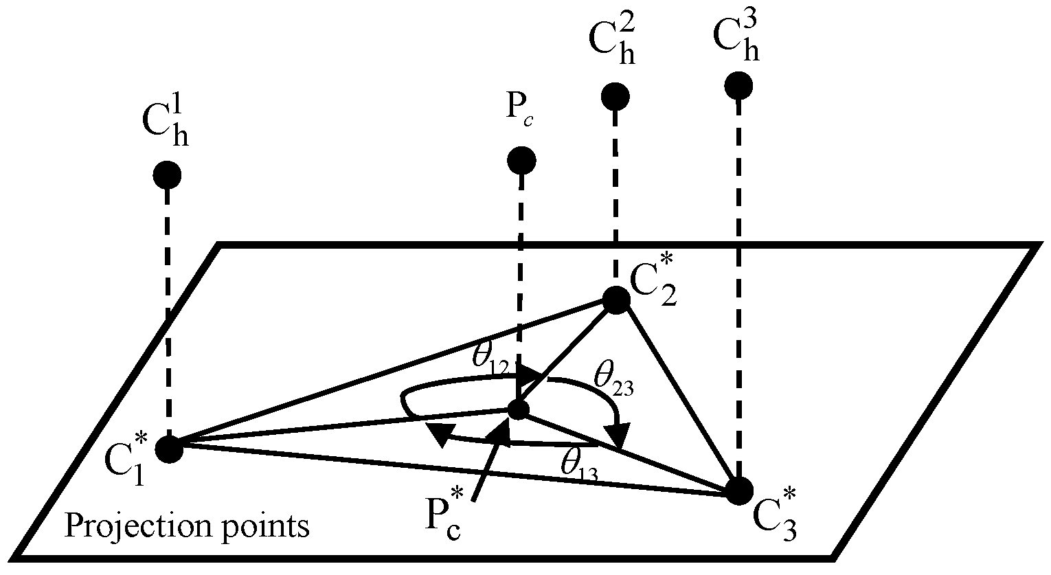
The primary surfaces (A1 on Part1 and A2 on Part2) must satisfy: (1) the minimum distance between A1 and A2 (Equation (4)), (2) a non-interference condition in assembly, and (3) the existence of at least three contact points under applied external forces. As illustrated in Figure 4, potential contact points C h 1 , C h 2 , and C h 3 , along with the force application point/centroid Pc, are projected onto the X-Y plane (denoted as C 1 * , C 2 * , C 3 * , and P c * ). The angular relationships between these projected points must satisfy Equations (4) and (5), where r1 represents the number of corresponding point pairs ( A 1 i , A 2 i ), n1 is the assembly direction vector, n A 2 i denotes the vertex normal vector of A 2 i , and T r / T t are the rotation/translation matrices, respectively.
min f = i = 1 N T r A 1 i + T t A 2 i n 1 2 s . t . T r A 1 i + T t A 2 i n A 2 i 0 ,   i = 1 , 2 , r 1 θ 12 + θ 23 + θ 13 = 360
θ 12 = arccos P c * C 1 * P c * C 2 * | P c * C 1 * | | P c * C 2 * | θ 23 = arccos P c * C 2 * P c * C 3 * | P c * C 2 * | | P c * C 3 * | θ 13 = arccos P c * C 1 * P c * C 3 * | P c * C 1 * | | P c * C 3 * |
2.
Secondary Mating Surface Model
Each secondary surface pair (B1j on Part1 and B2j on Part2) must satisfy two conditions: (1) the existence of at least two distinct contact points (e.g., C v 1 and C v 2 ) and (2) a non-interference condition in assembly, as defined by Equation (6). In this formulation, r2 represents the number of corresponding point pairs, n2 is the assembly direction vector, and n B 2 j denotes the vertex normal vector of B 2 j .
min f = i = 1 N T r B 1 j + T t B 2 j n 2 2 s . t . T r B 1 j + T t B 2 j n B 2 j 0 ,   j = 1 , 2 , r 2
3.
The Constraint Relationship Model
The connection parameter T contact = T r T t = 1 δ z δ y d x δ z 1 δ x d y δ y δ x 1 d z 0 0 0 1 between surface pairs is jointly constrained by the primary (Feature Vector Set 1: T1) and secondary (Feature Vector Set 2: T2) surfaces, following Equation (7) [32].
T contact = T 1 T 2 = δ x = δ x 1 ( o r ) δ x 2 δ y = δ y 1 ( o r ) δ y 2 δ z = δ z 1 ( o r ) δ z 2 d x = d x 1 ( o r ) d x 2 d y = d y 1 ( o r ) d y 2 d z = d z 1 ( o r ) d z 2
The parameters { δ x , δ y , δ z } and { d x , d y , dz } represent rotational and translational vectors along the x-, y-, z- axes, while { δ x 1 , δ y 1 , δ z 1 }/{ d x 1 , d y 1 , dz 1 } and { δ x 2 , δ y 2 , δ z 2 }/{ d x 2 , d y 2 , dz 2 } denote vectors for Features 1 and 2, respectively. The operator indicates or based on Boolean operations between overlapping vectors.
Step 5: Model Solution
The iterative optimization began with initialization parameters (iteration count k = 0, initial error transformation matrices T r 0 = 0 and T t 0 = I , where I denotes the identity matrix). To address the multi-constraint assembly problem, a penalty function was formulated to convert the constrained optimization (Step 4) into an unconstrained form (Equation (8)), thereby enhancing computational stability and convergence. The surface registration model with coupled constraints was subsequently optimized using a hybrid particle swarm algorithm until the optimal solution T contact was achieved. The workflow is illustrated in Figure 2.
f ( T r , T t ) = f ( d x , d y , d z , δ x , δ y , δ z ) = v = 1 q W F d v ( u ) n o n int e r 2 + W int d v ( u ) int e r 2 W F = 1 d v 0 0 d v < 0 W int = 0 d v 0 50 d v < 0
where d v ( u ) represents the Euclidean distance between corresponding point pairs during iteration. d v ( u ) n o n i n t e r indicates the non-interference distance (when d v 0 , surfaces A1/B1 are interference-free with weight factor W F = 1 ; d v < 0 indicates interference with W F = 0 ). d v ( u ) i n t e r measures interference penetration depth ( d v 0 : no interference, W i n t = 0 ; d v < 0 : interference occurs, W i n t = 50 ).

2.2. Determination of Primary and Secondary Contact Points

Within the assembly coordinate system, the optimal solution T 1 contact is used to calculate the initial contact point positions on the part to be assembled (Part2) prior to registration, based on its post-registration contact point locations. Under stable assembly conditions, the proposed model provides the closest approximation to the physical solution.
A 2 m = T 1 contact C h
B 2 m = T 1 contact C v

2.3. Assembly Pose Calculation Method with Multi-Constraint Coupled Registration

2.3.1. Two-Dimensional Assembly Case

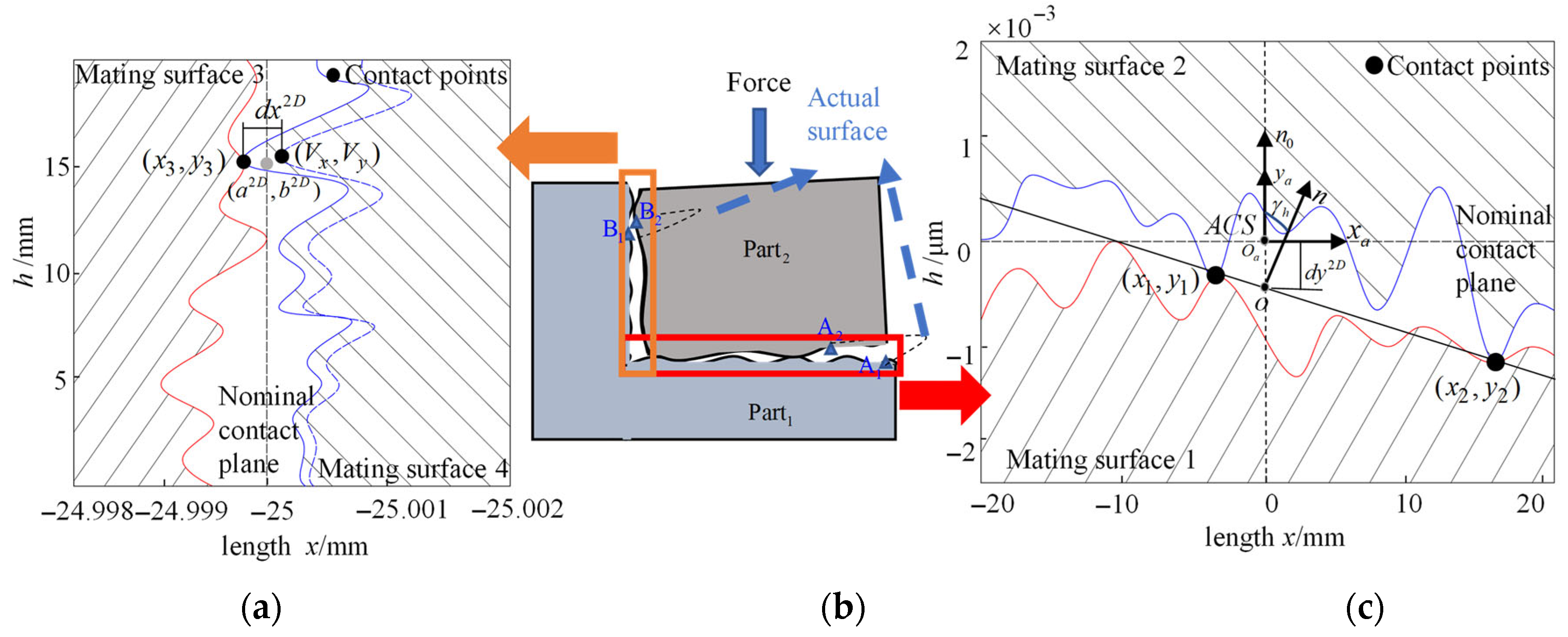
As detailed in Section 2.2, under vertical applied external forces, the horizontal surfaces act as the primary mating surfaces in this assembly case, while the vertical surfaces serve as the secondary ones. As shown in Figure 5, the assembly coordinate system (ACS) for the 2D mating surfaces is defined with its horizontal axis xa aligned with a pair of nominal horizontal contact lines. The vertical axis ya originates from the midpoint of the horizontal mating surface. Within the ACS, the contact points are designated as: C h 1 ( x 1 , y 1 ) and C h 2 ( x 2 , y 2 ) for the primary mating surfaces’ contact, and C v ( x 3 , y 3 ) for secondary mating surfaces’ contact.
  • Constraint Analysis of Primary Mating Surfaces
The equation of the realized contact line is given by:
y = y 1 y 2 x 1 x 2 x + [ y 2 x 2 ( y 1 y 2 ) x 1 x 2 ]
The angular deviation (γh) between this contact line and the nominal horizontal contact line (xa-axis) is calculated as:
γ h = arctan ( y 1 y 2 x 1 x 2 )
with a minor translational vector along the ya-axis expressed as:
d y 2 D = y 2 x 2 ( y 1 y 2 ) x 1 x 2
2.
Constraint Analysis of Secondary Mating Surfaces
The contact point on the vertical mating surface undergoes a slight translation along the xₐ-axis. In Figure 5, the nominal contact point is defined at coordinates ( a 2 D , b 2 D ) . However, its realized coordinates, denoted as (Vx, Vy), deviate from this nominal position due to constraints imposed on the horizontal surfaces. Here, the x-coordinate a 2 D = −25, indicating that the point lies on the nominal vertical contact line x = −25, while the y-coordinate b2D is an unknown variable. Solving Equation (14) yields the result given in Equation (15).
V = ( V x , V y , 1 ) T = ( V x , y 3 , 1 ) T = cos ( γ h ) sin ( γ h ) 0 sin ( γ h ) cos ( γ h ) d y 2 D 0 0 1 × ( a 2 D , b 2 D , 1 ) T
d x 2 D = V x x 3
3
Relative Pose Representation
Consequently, the relative pose variation of the mating surfaces A2 and B2 on the part2, relative to the nominal assembly, is described using a Small Displacement Torsor (SDT):
T 2 D = d x 2 D 0 d y 2 D 0 0 γ h

2.3.2. Three-Dimensional Assembly Case

As detailed in Section 2.2, under vertical applied external forces, the horizontal surfaces act as the primary mating surfaces, while the vertical surfaces serve as the secondary ones. The assembly coordinate system (ACS) for the 3D mating surfaces is illustrated in Figure 6. The plane xaoaya passes through the highest point of Mating Surface 1, defining the nominal mating plane. The origin oa is located at the geometric center of this nominal plane. The nominal position of the vertical mating surface is at x = −a3D (where a3D > 0), parallel to the y-z plane.
The contact points are defined as C h 1 ( x 1 , y 1 , z 1 ) , C h 2 ( x 2 , y 2 , z 2 ) , and C h 3 ( x 3 , y 3 , z 3 ) on the primary mating surfaces, and C v 1 ( x 4 , y 4 , z 4 ) , C v 2 ( x 5 , y 5 , z 5 ) on the secondary mating surfaces.
1.
Constraint Analysis of Primary Mating Surfaces
The equation of the realized horizontal mating surface is given by:
z = A x + B y + C
( x i , y i , 1 ) A B C = z i
The surface normal vector is expressed as:
n h = [ A , B , 1 ]
The angular deviation vectors of the realized mating surface relative to ACS (about x/y axes) are:
α 3 D = arccos n h e x n h e x
β 3 D = arccos n h e y n h e y
The minor translational displacement along the za-axis is:
d z 3 D = C
2
Constraint Analysis of Secondary Mating Surfaces
The spatial contact line equation for the Vertical Mating Surface is:
x x 4 x 5 x 4 = y y 4 y 5 y 4 = z z 4 z 5 z 4
The rotation angle about the z-axis ( γ 3 D ) and translational displacement in the x-direction (dx3D) are as follows:
The contact point on the vertical mating surface undergoes a slight translation along the xₐ-axis. Consistent with the principle established in the prior 2D assembly case analysis, the nominal contact point on this surface is defined by coordinates ( a 3 D , b 3 D , c 3 D ) . Here, a3D is a known quantity along the x-axis, while b3D and c3D are unknown. The realized coordinates of this point deviate from their nominal values due to the constraints applied on the horizontal surfaces. Solving Equation (25) yields the solution presented in Equation (26).
γ 3 D = arctan x 5 x 4 y 5 y 4
V 3 D = ( V x 3 D , V y 3 D , V z 3 D , 1 ) T = ( V x 3 D , y 4 , z 4 , 1 ) T = cos β 3 D cos γ 3 D cos β 3 D sin γ 3 D sin β 3 D 0 cos α 3 D sin γ 3 D + sin α 3 D sin β 3 D cos γ 3 D cos α 3 D cos γ 3 D sin α 3 D sin β 3 D sin γ 3 D sin α 3 D cos β 3 D 0 sin α 3 D sin γ 3 D cos α 3 D sin β 3 D cos γ 3 D sin α 3 D cos γ 3 D + cos α 3 D sin β 3 D sin γ 3 D cos α 3 D cos β 3 D d z 3 D 0 0 0 1 × ( a 3 D , b 3 D , c 3 D , 1 ) T
d x 3 D = V x 3 D x 4
3.
Relative Pose Representation
The resulting SDT matrix is:
T 3 D = d x 3 D α 3 D 0 β 3 D d z 3 D γ 3 D

3. Analysis of Registration States in 2D Assembly

The proposed multi-constraint coupled registration method is demonstrated through specific case studies. This section details the registration states and results from 2D assemblies under two distinct loading conditions: a vertical applied external force and a horizontal applied external force.

3.1. Assembly Under a Vertical Applied External Force

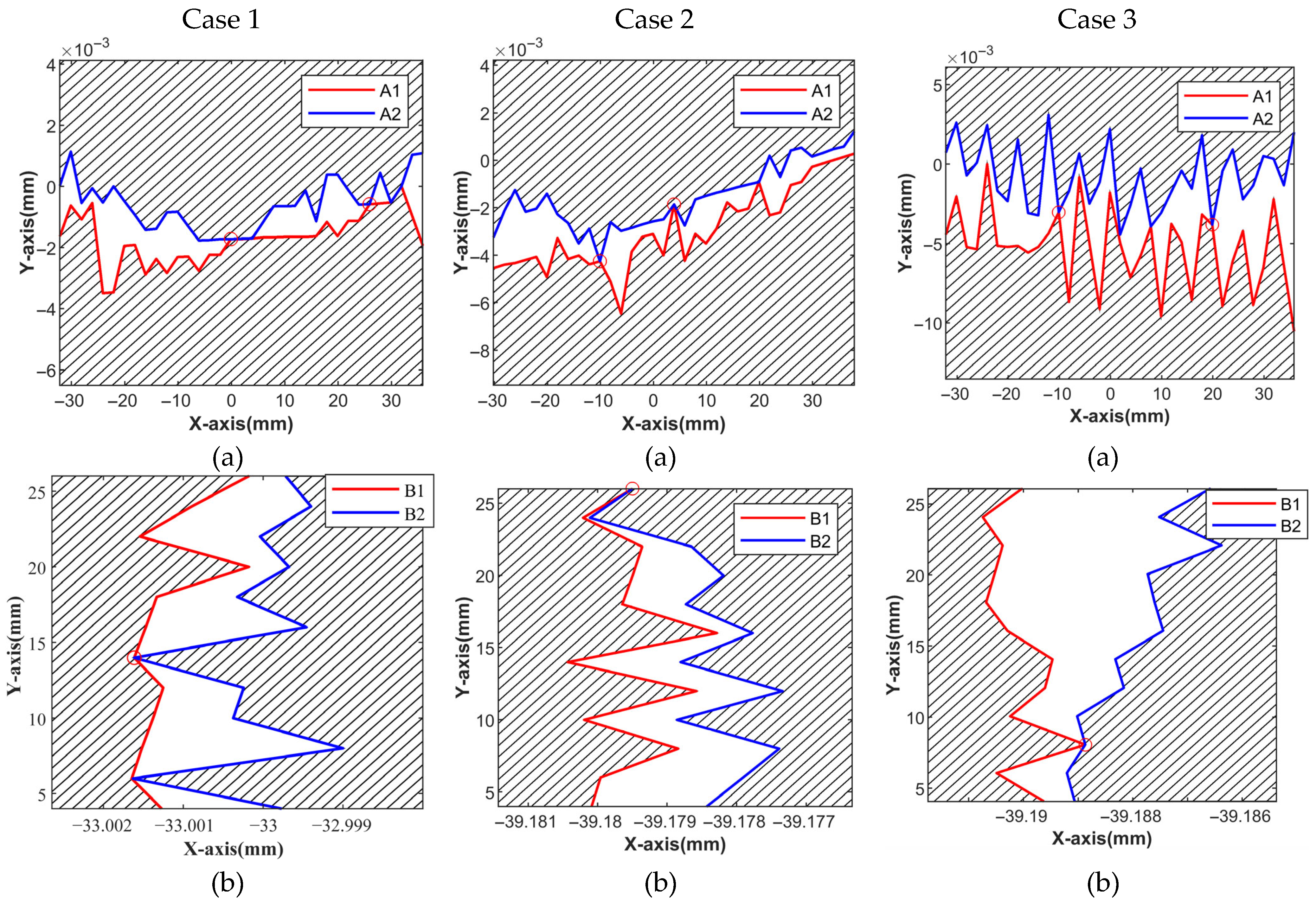
Figure 7 displays three groups of 2D mating examples for the 2D-Case 1-3 under a vertical applied external force, demonstrating different geometric distribution errors of the part mating surfaces. Each part has two mating surfaces: one horizontal (e.g., 2D-Case 1(a) in Figure 7) and one vertical (e.g., 2D-Case 1(b) in Figure 7).
The corresponding registration results for the 2D-Case 1-3, computed using the proposed method, are depicted in Figure 8. A key observation is that under the vertical applied external force, the horizontal mating surfaces act as the primary mating surfaces, while the vertical ones are secondary. Moreover, two pairs of contact points are determined on the horizontal surfaces, whereas only one pair exists on the vertical surfaces. Based on the multi-constraint coupled model, the parts achieved a stable equilibrium. Quantitative data for this configuration are summarized in Table 1 (see 2D-Case 1–3).

3.2. Assembly with a Horizontal Applied External Force

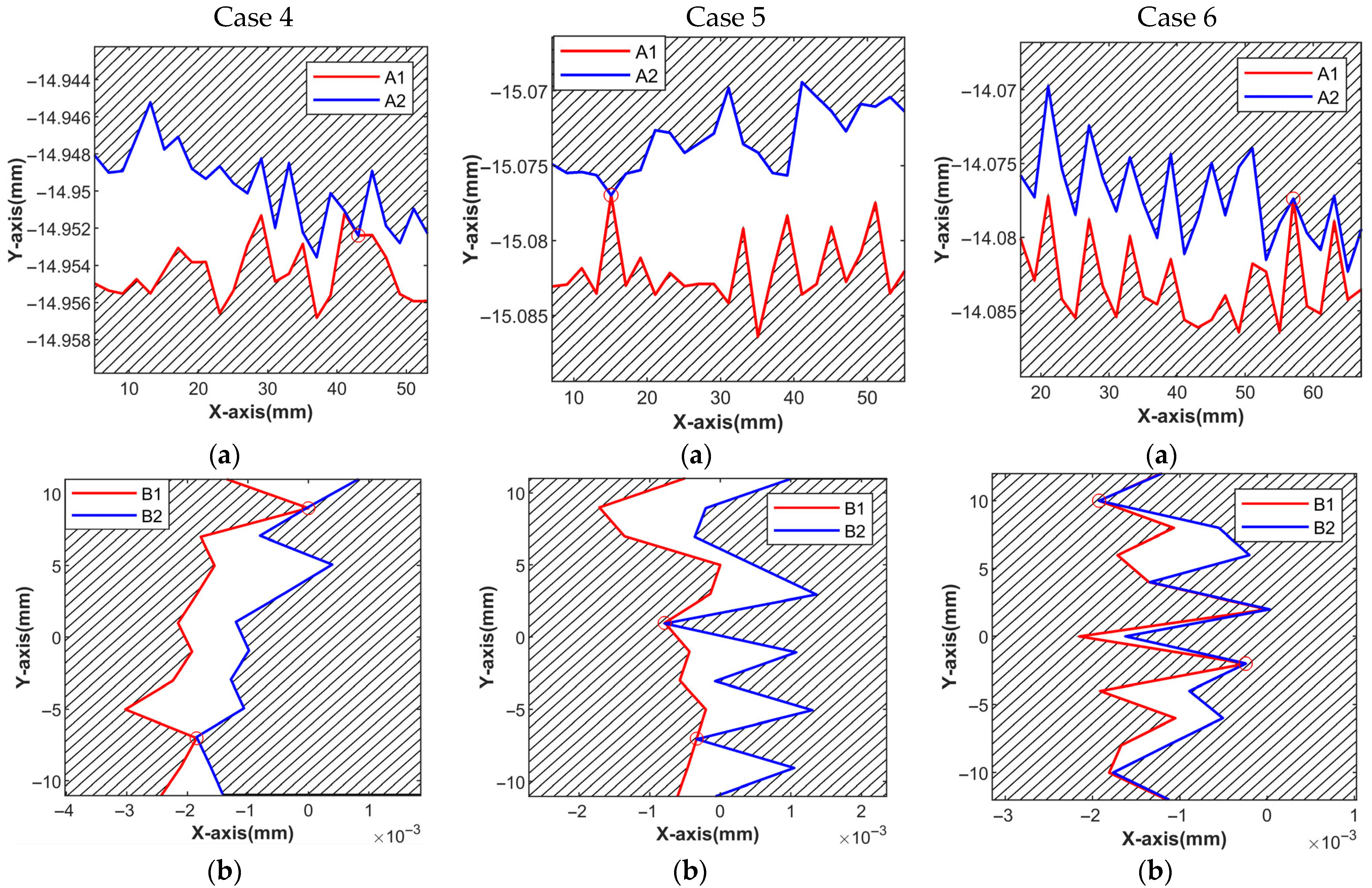
To further validate the repeatability of the proposed method, its performance was evaluated under a rightward horizontal applied external force, a scenario distinct from the vertical loading case detailed in Section 3.1. The testing involved components with differing geometric distribution errors. Their initial poses and geometric distribution errors are provided in Figure 9.
The registration results for the three groups of parts under the horizontal applied external force are shown in Figure 10. A distinct trend is observed across all groups: the vertical mating surfaces now bear more contact pairs, with two pairs determined on them, while the horizontal surfaces exhibit one pair. By incorporating the applied force into the model, the proposed method captures this resulting shift in contact patterns and the consequent change in the part’s final pose, as evidenced by the reversal when compared to the vertical applied external force cases (Figure 8). This demonstrates its capability to predict the contact points and stable poses under varying load conditions. This outcome is quantitatively confirmed by the data in Table 1 (see 2D-Case 4–6).

4. Three-Dimensional Surface Registration Experiment

To validate the effectiveness of the proposed method based on geometric distribution errors, we designed experiments using plane–plane mating structures with machine tool tailstock mock-ups.

4.1. Experimental Setup

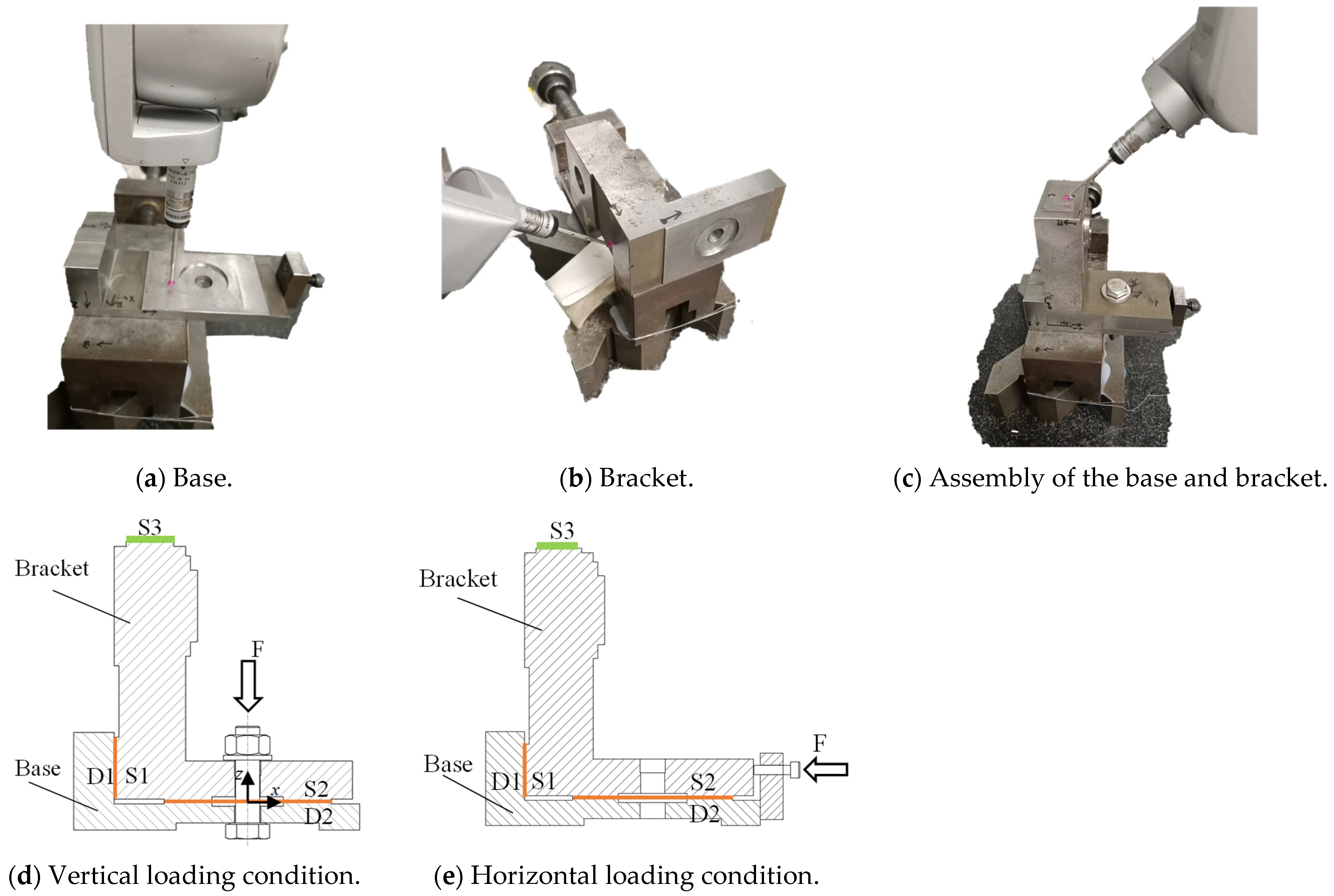
The apparatus primarily consists of a base and an L-shaped bracket (Figure 11). The experimental components were constructed from Grade 45 steel, a common material in mechanical structures. This material selection supports the validation of the model’s applicability to components made of other similarly rigid materials. The mating surfaces (Base: side D1 and horizontal plane D2; Bracket: side S1 and horizontal plane S2) were then milled according to the specifications given in Table 2.

4.2. Experimental Scheme

The experimental measurement process is illustrated in Figure 12a–c. First, prior to assembly, a coordinate measuring machine (CMM; model: Global 5.7.5, manufacturer: Hexagon Manufacturing Intelligence, Qingdao, China) with a measurement uncertainty of (1.7 + 3L/1000) μm was used to acquire surface point cloud data for the bracket’s side (S1), horizontal (S2), and top (S3) planes. A total of 12 rows with 25 points each were collected on the side surface of the bracket; 24 rows comprising 643 points were obtained on the horizontal surface; and 30 points were captured on the top surface. The number of points was determined by the sampling interval, which was set between 2 mm and 4 mm in this study. Measurements were performed using PC-DMIS 2018 software.
Subsequently, the side (D1) and horizontal (D2) planes of the base were measured. The measurement strategy for the base surfaces was consistent with that used for the bracket, with 300 points collected on the side surface and 643 points on the horizontal surface. All measurements were conducted following CMM calibration, with errors primarily dependent on the equipment’s inherent accuracy. The orientation of the measurement coordinates is shown in Figure 12d. For the base, the coordinate system origin was located at the geometric center of the horizontal surface, with the positive x-axis directed to the right and the positive Z-axis oriented vertically upward.
Following the part measurement phase, the components were assembled according to the procedure described later in this section. To determine the spatial pose of the assembled bracket, a global assembly coordinate system was established coincident with the base coordinate system. The pose of the bracket’s top surface (S3) was then measured within this assembly frame, consisting of 6 rows with 5 points each (30 points total). To ensure experimental repeatability, components from Table 2 were assembled in different combinations under two loading conditions: vertical (Figure 12d) and horizontal (Figure 12e). Three experimental trials were conducted for each loading condition using different component sets, resulting in a total of six experimental tests, as summarized in Table 3.
The assembly procedure involved: (1) The bracket was positioned on the base. Relying on gravity and rough alignment, the horizontal mating surfaces (D2–S2) were brought into initial contact, while the side surfaces (D1–S1) were approximately aligned and contact. (2) A bolt was inserted and hand-tightened until slight resistance was felt. Subsequently, a small initial torque was applied using a torque wrench, which was just sufficient to maintain part contact while still permitting fine adjustments. (3) Fine-tuning was performed by gently tapping the sides and ends of the bracket with a plastic hammer until the operator tactually and visually confirmed that both mating surface pairs were in full contact. (4) Finally, the bolt was tightened to the specified target torque using the torque wrench, locking the assembly in its final position. For the vertical loading condition, the final torque was 150 N·cm, while for the horizontal loading condition, it was 12 N·cm (within a range of 11.6–13 N·cm).
Subsequently, the proposed method is employed to predict the point cloud P′(xs′, ys′, zs′) representing the pose of the top surface S3. Finally, the measured values Pa(xs, ys, zs) of S3 are compared with the predicted values P′(xs′, ys′, zs′).

4.3. Analysis of 3D Surface Registration States

The 3D registration results under different loading conditions are presented in Section 4.3.1 and Section 4.3.2. Detailed quantitative data supporting these observations are provided in Appendix A (Table A1).
The predicted assembled pose of the target surface was calculated according to the following procedure: First, the spatial pose transformation matrix MP was constructed from the SDT parameters (determined in Section 2.3) using Equation (28). Subsequently, the point cloud P(x, y, z) was transformed into the predicted assembled point cloud P’ by applying the matrix operation defined in Equation (29), thereby obtaining the predicted pose.
M P = M t r a n s l a t i o n M z M y M x = 1 0 0 d x 3 D 0 1 0 d y 3 D 0 0 1 d z 3 D 0 0 0 1 cos γ 3 D sin γ 3 D 0 0 sin γ 3 D cos γ 3 D 0 0 0 0 1 0 0 0 0 1 cos β 3 D 0 sin β 3 D 0 0 1 0 0 sin β 3 D 0 cos β 3 D 0 0 0 0 1 1 0 0 0 0 cos α 3 D sin α 3 D 0 0 sin α 3 D cos α 3 D 0 0 0 0 1
P = M P P

4.3.1. Registration Under Vertical Applied External Force

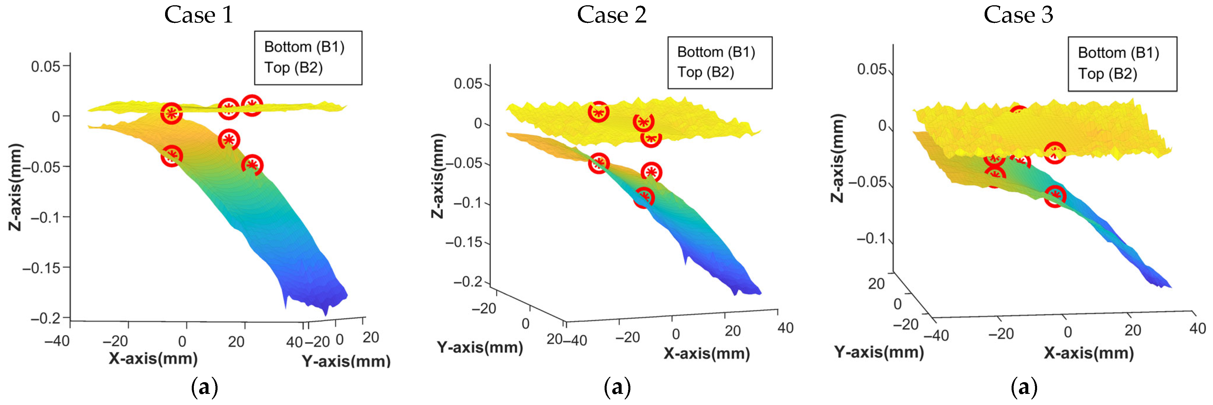
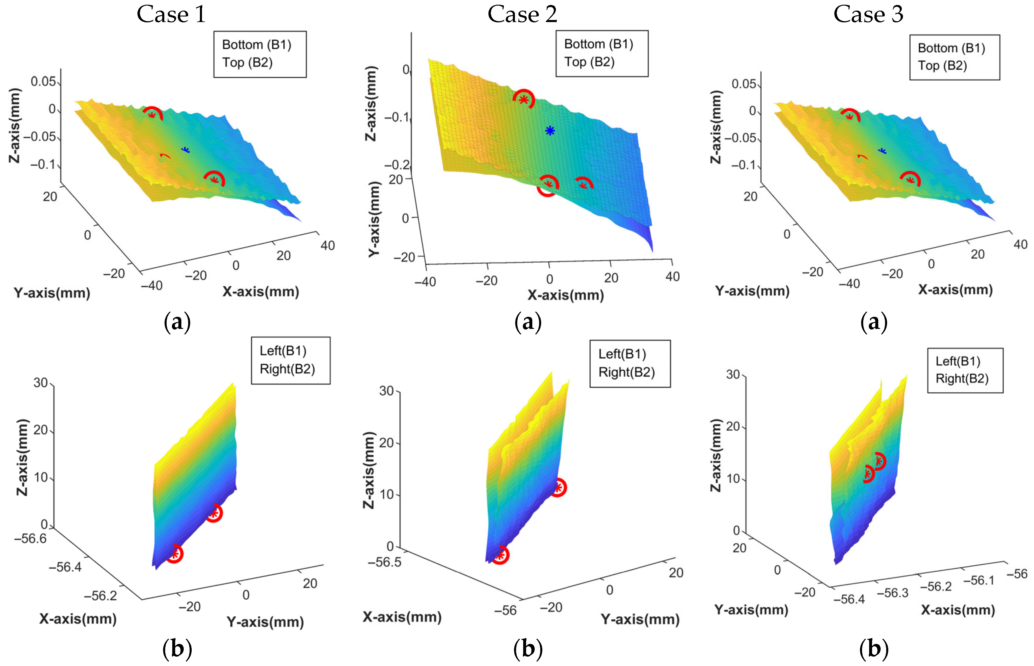
Figure 13 illustrates the initial state of three groups of 3D mating surfaces under a vertical applied external force (3D-Case 1-3), as well as the variations in geometric distribution errors on different part surfaces. In this scenario, the proposed method determined the horizontal surface to be the primary constraint, with the side surface as the secondary constraint. The red dots in Figure 13, such as 3D-Case 1(a) and 3D-Case 1(b), indicate the predicted contact points prior to registration, which are calculated from Equations (9) and (10).
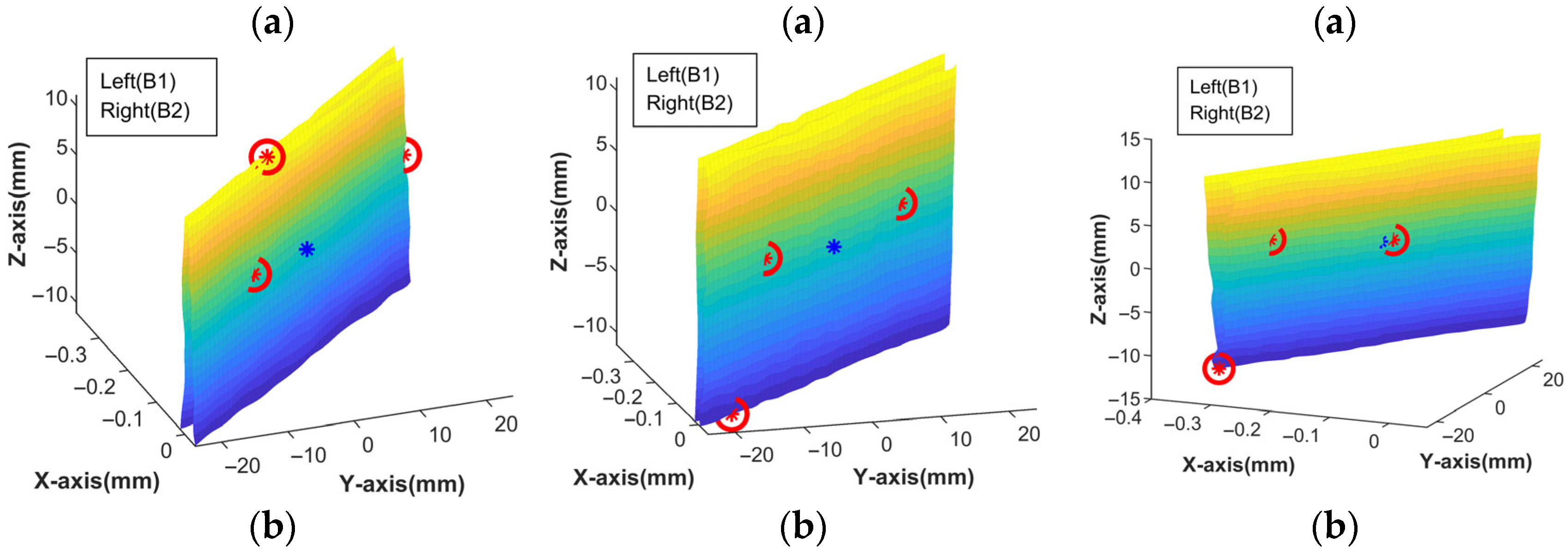
Corresponding to the initial states in Figure 13, Figure 14 illustrates the resultant pose of the mating surfaces and the distribution of contact points predicted by the proposed method. It is observed that the component settles into a stable pose where the horizontal surfaces, as expected, provide the primary constraint. Meanwhile, the contact points on the side surfaces adjust to compensate for geometric distribution errors, fulfilling a secondary constraining role. This result confirms that the proposed method can determine the contact points and predict the assembly state under vertical loading.

4.3.2. Registration Under Horizontal Applied External Force

The initial states for the horizontal applied external force (3D-Case 4-6) are shown in Figure 15. This figure shares the same geometric distribution errors as Figure 13 (see Table 3), but with a differing load condition. In this scenario, the proposed method re-prioritizes the constraints, designating the side surfaces as primary and the horizontal surfaces as secondary.
As shown in Figure 16, the final assembly state differs from that under the vertically applied external force. This validates that forces acting on surfaces with geometric distribution errors directly influence part contact state. In this case, the force also alters the constraint priority of the mating surface, wherein the side surfaces act as the primary constraint. The capability to predict stable assembly states, which accounts for both geometric distribution errors and applied external forces, provides a solution for assessing assembly poses.

4.4. Experimental Results

The relative errors between predicted and experimentally measured values of S3 were calculated using Equation (30), with results presented in Table 4.
RMSE = s = 1 k ( P a P ) 2 P a = s = 1 k ( x s x s ) 2 + ( y s y s ) 2 + ( z s z s ) 2 ( x s ) 2 + ( y s ) 2 + ( z s ) 2
In the equation, k represents the number of measurement points.

4.5. Results and Discussion

Figure 13 reveals the geometrical distribution errors, characterized by spatial undulations, present on the mating surfaces under specific machining conditions. As these error surfaces are reconstructed from measurement data, their morphology closely aligns with that of the actual workpiece [30], thereby establishing a foundation for the model. Following the stable assembly of the two pairs of mating surfaces, Figure 14 demonstrates that the spatial position of the contact points influences the final pose of the assembly. This stands in stark contrast to conventional tolerance-based methods, which can only predict a range of variations but fail to ascertain the actual contact point locations or the resulting registered state. This fundamental discrepancy arises because traditional methods operate on idealized tolerance zones, which lack the topographical detail to resolve specific contact behavior. In contrast, our model, by leveraging the actual geometrical distribution, bridges this gap by simulating the physical contact interactions that ultimately define the assembly pose.
Furthermore, achieving accurate predictions for the assembly of complex, multi-constrained components necessitates considering not only these geometrical distribution errors but also assembly process parameters, particularly applied external forces. Two distinct predictions for the final part pose and contact points are obtained from a comparison of Figure 14a and Figure 16a, which use the same experimental setup, under different loading conditions. A model that neglects the influence of applied external forces would be incapable of distinguishing between these states and would produce a single prediction. The divergence in predicted poses demonstrates that the applied force alters the sequence and conditions of contact establishment, thereby guiding the assembly into different stable configurations. Consequently, capturing this force-dependent behavior is essential for predictive accuracy.
In conclusion, the proposed multi-constraint coupling model, which integrates geometrical distribution errors and critical assembly parameters, transitions assembly prediction from a purely geometric domain into a physically grounded simulation. As validated by the experimental data in Table 4, this method provides a quantitative solution for predicting the state of complex assemblies. The method could be extended to complex non-planar assemblies. Such an extension would not change the model but would depend on the data acquisition, data pre-processing, and dimensionality reduction of data from curved surfaces.

5. Conclusions

In product assembly, geometric distribution errors from machined surfaces and the coupling of multiple mating surface constraints are critical factors affecting precision. To address this challenge, this paper proposes a method for predicting key assembly outcomes, including the final pose and contact points.
Based on measured data of mating surfaces, the method utilizes the NURBS method to characterize the geometric distribution errors of parts. Integrated with a priority-based theory for multi-surface assembly, a hierarchical surface registration model was developed. This model comprehensively accounts for the effects of geometric distribution errors, multi-constraint coupling, and applied external forces, thereby enabling it to predict the spatial poses of assembled components and provide a theoretical foundation for predicting product assembly accuracy.
Model validation was conducted through progressive case studies, from 2D to 3D. The 2D cases provided an intuitive analysis of the contact state between two mating surface pairs, determining contact point locations. Subsequently, six sets of assembly experiments were conducted. These experiments determined the contact point positions and the final poses of the mating surfaces for each assembly under two distinct loading conditions. The results demonstrated that the root mean square error (RMSE) between the predicted and measured values for the critical surface parameters was less than 2%.

Author Contributions

All authors contributed to the study’s conception and design. L.L. designed and conducted the experiments, analyzed the results, and wrote the article. X.J. proposed the basic idea of the article and contributed the materials and measuring instruments. C.L. modified the structure of the article. H.G. helped perform the analysis with constructive discussions. All authors have read and agreed to the published version of the manuscript.

Funding

The work was supported by the National Natural Science Foundation of China (grant number U22B2088).

Institutional Review Board Statement

Not applicable.

Informed Consent Statement

Not applicable.

Data Availability Statement

The original contributions presented in this study are included in the article. Further inquiries can be directed to the corresponding author.

Conflicts of Interest

The authors declare no conflicts of interest.

Appendix A

Table A1. Experimental Results and Analysis of the 3D Assembly.
Case
(3D-Case)
Mapping Matrix MContact Points of the
Assembly Coordinate System D1 and D2
SDT
Horizontal Mating Surfaces A1 and A2;
Side Surfaces B1 and B2
1 M = 1 0 0 0 . 0066 0 1 0 0 0 0 1 0 . 0844 0 0 0 1 A1(−3.9990, 15.9993, −0.0276) T 3 D = 0 . 1788 0 . 0002 0 0 . 0024 0 . 0477 0 . 0077
(−5.9988, −22.0010, −0.0394)
(4.0006, 15.9989, −0.0528)
B1(−56.4066, 9.9989, 4.0006)
(−56.2184, −14.0006, 4.0012)
A2(−4.1066, 16.0010, 0.0030)
(−6.1066, −21.9992, 0.0028)
(3.8933, 16.0009, 0.0066)
B2(−56.0979, 9.9989, 4.0007)
(−56.0931, −14.0007, 4.0013)
2 M = 1 0 0 0 . 0298 0 1 0 0 0 0 1 0 . 0750 0 0 0 1 A1(−3.9990, 15.9993, −0.0276)
(0.0009, −22.0015, −0.0535)
(12.0016, −14.0010, −0.0917)
T 3 D = 0 . 1820 0 . 0003 0 0 . 0030 0 . 0215 0 . 0077
B1(−56.1899, −18.0005, 4.0102)
(−56.5116, 23.9998, 4.0099)
A2(−4.1233, 15.9963, 0.0174)
(−0.1218, −22.0024, 0.0117)
(11.8787, −14.0026, 0.0048)
B2(−56.1308, −18.0005, 4.0102)
(−56.1484, 23.9998, 4.0099)
3 M = 1 0 0 0 . 0031 0 1 0 0 0 0 1 0 . 0829 0 0 0 1 A1(−7.9985, 16.0005, −0.0145)
(0.0016, −16.0001, −0.0262)
(−15.9982, −5.9998, −0.0167)
T 3 D = 0 . 1202 0 . 00005 0 0 . 0007 0 . 0117 0 . 0073
B1(−56.1897, 2.0002, 16.0107)
(−56.2479, −6.0002, 16.0103)
A2(−2.0607, 17.9965, 0.0141)
(−0.0599, −16.0028, 0.0125)
(−16.0603, −6.0033, 0.002)
B2(−56.0777, 2.0002, 16.0107)
(−56.0749, −6.0002, 16.0103)
4 M = 1 0 0 0 . 0366 0 1 0 0 0 0 1 0 . 0344 0 0 0 1 A1(−0.0839, −10.0002, 1.0230)
(−0.3464, 23.9989, 1.0236)
(−0.1286, −6.0009, 11.0485)
T 3 D = 0 . 1591 0 . 0001 0 0 . 0014 0 . 0373 0 . 0077
B1(40.1562, −24.0009, −15.0786)
(40.1563, 19.9992, −15.0731)
A2(0.0314, −10.0002, 1.023)
(0.0206, 23.9989, 1.0236)
(0.0061, −6.0009, 11.0485)
B2(40.0493, −23.9815, −14.987)
(40.0488, 20.0175, −14.9663)
5 M = 1 0 0 0 . 0202 0 1 0 0 0 0 1 0 . 0280 0 0 0 1 A1(−0.0711, −11.9999, 0.9542)
(−0.2694, 14.0002, 0.9539)
(−0.0348, −18.0005, −11.0463)
T 3 D = 0 . 1618 0 . 0003 0 0 . 0009 0 . 0131 0 . 0077
B1(34.1562, 13.9988, −15.0622)
(34.1561, −14.0012, −15.0731)
A2(0.0152, −11.9999, 0.9542)
(0.0051, 14.0002, 0.9539)
(0.0243, −18.0005, −11.0463)
B2(34.0328, 13.9977, −15.0402)
(34.0331, −14.003, −15.0446)
6 M = 1 0 0 0 . 0831 0 1 0 0 0 0 1 0 . 0233 0 0 0 1 A1(−0.286, −24.0002, −10.7048)
(−0.0978, 2.0002, 1.2955)
(−0.2324, −15.9998, 3.2949)
T 3 D = 0 . 1111 0 . 00004 0 0.0004 0 . 0009 0 . 0075
B1(40.0939, −5.9998, −14.7811)
(48.0936, 16.0005, −14.7789)
A2(0.0237, −24.0002, −10.7048)
(0.0145, 2.0002, 1.2955)
(0.0128, −15.9998, 3.2949)
B2(40.0318, −5.9876, −14.7164)
(48.0325, 16.0123, −14.6902)

References

  1. Guo, H.; Zhang, Z.; Xiao, M.; Liu, H.; Zhang, Q. Tolerance optimization method based on flatness error distribution. Int. J. Adv. Manuf. Tech. 2021, 113, 279. [Google Scholar] [CrossRef]
  2. Saren, Q.; Zhang, Z.; Xiong, J.; Chen, X.; Zhu, D.; Wu, W.; Jin, X.; Shang, K. An accuracy and performance-oriented accurate digital twin modeling method for precision microstructures. J. Intell. Manuf. 2024, 35, 2887–2911. [Google Scholar] [CrossRef]
  3. Jiang, Q.; Feng, H.; Wang, Y.; Fang, C. Batch circular form error characterization and evaluation. Precis. Eng. 2017, 47, 223–230. [Google Scholar] [CrossRef]
  4. Mantripragada, R.; Whitney, D.D.E. The Datum Flow Chain: A Systematic Approach to Assembly Design and Modeling. Res. Eng. Des. 1998, 10, 150–165. [Google Scholar] [CrossRef]
  5. Camelio, J.; Hu, S.J.; Ceglarek, D. Modeling Variation Propagation of Multi-Station Assembly Systems with Compliant Parts. J. Mech. Des. 2003, 125, 673–681. [Google Scholar] [CrossRef]
  6. Anselmetti, B.; Mejbri, H.; Mawussi, K. Coupling experimental design—Digital simulation of junctions for the development of complex tolerance chains. Comput. Ind. 2003, 50, 277–292. [Google Scholar] [CrossRef]
  7. Anselmetti, B. Generation of functional tolerancing based on positioning features. Comput. Aided Des. 2006, 38, 902–919. [Google Scholar] [CrossRef]
  8. Lyu, C.; Liu, Z.; Ai, Y.; Yu, Z. Assembly Joint Surface Error Modeling and Tolerance Optimization in the Case of Coupled Tolerance. J. Mech. Eng. 2015, 51, 108–118. [Google Scholar] [CrossRef]
  9. Ke, J.; Jianhua, L.; Ruxin, N.; Chongying, G. Variation Analysis and Assembly Success Rate Computation for Clearance Fit under Constraint of Location Priority. J. Mech. Eng. 2014, 50, 136. [Google Scholar] [CrossRef]
  10. Hu, M.; Lai, X.M.; Lin, Z.Q.; Cheng, G.L.; Gan, P.; Zhu, J.H.; Zhou, L.B. Variation Analysis for Multi-Flexible Autobody Assembly. J. Shanghai Jiaotong Univ. 2000, 34, 1365–1368. [Google Scholar] [CrossRef]
  11. Mansuy, M.; Giordano, M.; Hernandez, P. A Generic Method for the Worst Case and Statistical Tridimensional Tolerancing Analysis. Procedia CIRP 2013, 10, 276–282. [Google Scholar] [CrossRef]
  12. Ding, S.; Zheng, X.; Bao, J.; Zhang, J. An improved Jacobian-Torsor model for statistical variation solution in aero-engine rotors assembly. Proc. Inst. Mech. Eng. Part B J. Eng. Manuf. 2021, 235, 466–483. [Google Scholar] [CrossRef]
  13. Zeng, W.; Rao, Y.; Wang, P.; Yi, W. A solution of worst-case tolerance analysis for partial parallel chains based on the Unified Jacobian-Torsor model. Precis. Eng. 2017, 47, 276–291. [Google Scholar] [CrossRef]
  14. Sun, J.; Siyi, D.; Zhimin, L.; Fuyong, Y.; Xun, M. Point-based solution using Jacobian-Torsor theory into partial parallel chains for revolving components assembly. J. Manuf. Syst. 2018, 46, 46–58. [Google Scholar] [CrossRef]
  15. Ding, S.; Zheng, X. Variation Analysis Considering the Partial Parallel Connection in Aero-Engine Rotor Assembly. Energies 2022, 15, 4451. [Google Scholar] [CrossRef]
  16. Besl, P.; McKay, N.D. Method for Registration of 3-D Shapes. In Proceedings of the Sensor Fusion IV: Control Paradigms and Data Structures, Boston, MA, USA, 12–15 November 1991; pp. 586–606. [Google Scholar] [CrossRef]
  17. Hu, X.; Zhao, Q.; Yang, Y.; Wan, S.; Sun, Y.; Hong, J. Accuracy analysis for machine tool spindles considering full parallel connections and form errors based on skin model shapes. J. Comput. Des. Eng. 2023, 10, 1970–1987. [Google Scholar] [CrossRef]
  18. Shen, T.; Lu, C. An assembly accuracy analysis approach of mechanical assembly involving parallel and serial connections considering form defects and local surface deformations. Precis. Eng. 2024, 88, 44–64. [Google Scholar] [CrossRef]
  19. Sangnui, S.; Peters, F. The Impact of Surface Errors on the Location and Orientation of a Cylindrical Workpiece in a Fixture. J. Manuf. Sci. Eng. 2001, 123, 325–330. [Google Scholar] [CrossRef]
  20. Lee, N.K.S.; Yu, G.H.; Chen, J.Y.; Joneja, A. Effect of Mechanical Alignment System on Assembly Accuracy. J. Manuf. Sci. Eng. 2003, 125, 595–608. [Google Scholar] [CrossRef]
  21. Lee, N.K.S.; Chen, J.Y.; Joneja, A. Effects of surface roughness on multi-station mechanical alignment processes. J. Manuf. Sci. Eng. 2001, 123, 433–444. [Google Scholar] [CrossRef]
  22. Lee, N.K.S.; Yu, G.; Joneja, A.; Ceglarek, D. The modeling and analysis of a butting assembly in the presence of workpiece surface roughness and part dimensional error. Int. J. Adv. Manuf. Tech. 2006, 31, 528–538. [Google Scholar] [CrossRef]
  23. Pierce, R.S.; Rosen, D. A Method for Integrating Form Errors Into Geometric Tolerance Analysis. J. Mech. Des. 2008, 130, 467–478. [Google Scholar] [CrossRef]
  24. Shang, K.; Wu, T.; Jin, X.; Zhang, Z.; Li, C.; Liu, R.; Wang, M.; Dai, W.; Liu, J. Coaxiality prediction for aeroengines precision assembly based on geometric distribution error model and point cloud deep learning. J. Manuf. Syst. 2023, 71, 681–694. [Google Scholar] [CrossRef]
  25. Zhang, J.; Qiao, L. Research on computing position and orientation deviations caused by mating two non-ideal planes. Procedia CIRP 2018, 75, 309–313. [Google Scholar] [CrossRef]
  26. Schleich, B.; Wartzack, S. Novel approaches for the assembly simulation of rigid Skin Model Shapes in tolerance analysis. Comput. Aided Des. 2018, 101, 1–11. [Google Scholar] [CrossRef]
  27. Wang, J.W.J.; Duan, L.D.L. A Direct Calculating Method and Experiment of Absolute Orientation for Unmanned Aerial Vehicle Photograph. Appl. Mech. Mater. 2013, 353–356, 3468. [Google Scholar] [CrossRef]
  28. Samper, S.; Adragna, P.; Favreliere, H.; Pillet, M. Modeling of 2D and 3D Assemblies Taking into Account Form Errors of Plane Surfaces. J. Comput. Inf. Sci. Eng. 2009, 9, 41005. [Google Scholar] [CrossRef]
  29. Daniel, F.; Weill, R.; Bourdet, P. Computer Aided Tolerancing and Dimensioning in Process Planning. ClRP Ann. 1986, 3511, 381–386. [Google Scholar] [CrossRef]
  30. Zhang, Z.; Zhang, Z.; Jin, X.; Zhang, Q. A novel modelling method of geometric errors for precision assembly. Int. J. Adv. Manuf. Tech. 2018, 94, 1139–1160. [Google Scholar] [CrossRef]
  31. Liu, X.L.; Zhang, X.D.; Fang, F.Z.; Liu, S.G. Identification and compensation of main machining errors on surface form accuracy in ultra-precision diamond turning. Int. J. Mach. Tools Manuf. 2016, 105, 45–57. [Google Scholar] [CrossRef]
  32. Chen, H.; Jin, S.; Li, Z.; Lai, X. A solution of partial parallel connections for the unified Jacobian-Torsor model. Mech. Mach. Theory 2015, 91, 39–49. [Google Scholar] [CrossRef]
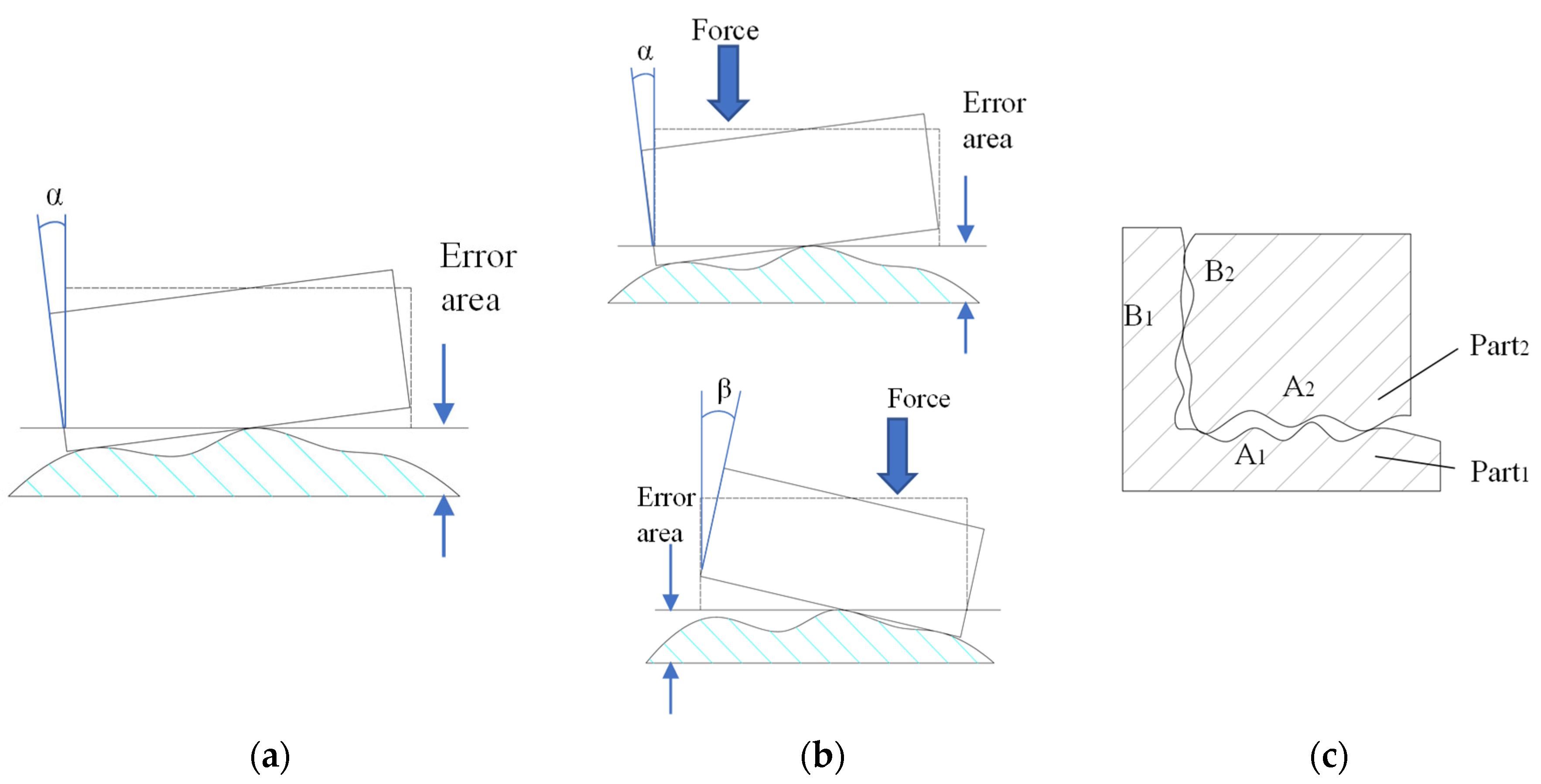
Figure 1. Key factors influencing the assembled pose in this study. The schematic illustrates the effects of (a) geometric distribution errors, (b) applied external force (under identical geometric distribution errors, left-side applied force induces leftward pose inclination while right-side applied force causes rightward inclination), and (c) multi-surface constraint coupling on the final assembled pose.
Machines 13 01009 g001
Figure 2. Registration method with coupled multi-constraints considering geometric distribution errors.
Machines 13 01009 g002
Figure 3. Schematic of the assembly state for two pairs of mating surfaces. (a) Two-dimensional assembly schematic. Under ideal conditions, the parts contact at their nominal positions. In the presence of geometric distribution errors, the mating surfaces contact at discrete points, resulting in angular deviation. (b) Three-dimensional assembly schematic, illustrating how geometric distribution errors on the two pairs of mating surfaces collectively determine their final assembly pose. Labels A1/A2 and B1/B2 denote the primary and secondary mating surface pairs, respectively. The arrow indicates the applied external force.
Machines 13 01009 g003
Figure 4. Projection diagram.
Machines 13 01009 g004
Figure 5. Assembly pose and contact state for the 2D case. (a) Contact state on the secondary mating surfaces (B1, B2). (b) Schematic of the component’s overall assembly pose resulting from the coupled constraints. (c) Contact state on the primary mating surfaces (A1, A2). The contact points on each surface pair are linked to the multi-constraint assembly pose. Solid red and blue lines in (a,c) depict the as-manufactured profiles of Mating Surfaces 1–4. The dashed blue line indicates the realized profile after translation, resulting from constraints on the horizontal surfaces, showing the shift of the contact point from its nominal position (a2D, b2D) to the realized position (Vx, Vy).
Machines 13 01009 g005
Figure 6. Assembly pose and contact state for the 3D case. (a) Contact state on the secondary mating surfaces (B1, B2). (b) Schematic of the component’s overall assembly pose resulting from the coupled constraints. The orange and red brackets highlight the regions corresponding to the secondary (a) and primary (c) mating surfaces, respectively. (c) Contact state on the primary mating surfaces (A1, A2). The contact points on each surface pair are linked to the multi-constraint assembly pose.
Machines 13 01009 g006
Figure 7. Examples of 2D registration under a vertical applied force. The three columns represent Case 1, Case 2, and Case 3, respectively. (a) illustrates horizontal mating surfaces and (b) shows vertical mating surfaces. The red circle highlights the location of the contact point.
Machines 13 01009 g007
Figure 8. Registration results for 2D mating surfaces under a vertical applied force. The three columns represent Case 1, Case 2, and Case 3, respectively. (a) illustrates horizontal mating surfaces and (b) shows vertical mating surfaces. The red circle highlights the location of the contact point.
Machines 13 01009 g008
Figure 9. Examples of 2D registration under a horizontal applied force. The three columns represent Case 4, Case 5, and Case 6, respectively. (a) demonstrating horizontal mating surfaces and (b) showing vertical mating surfaces. The red circle highlights the location of the contact point.
Machines 13 01009 g009aMachines 13 01009 g009b
Figure 10. Registration results for 2D mating surfaces under a horizontal applied force. The three columns represent Case 4, Case 5, and Case 6, respectively. (a) demonstrating horizontal mating surfaces and (b) shows vertical mating surfaces. The red circle highlights the location of the contact point.
Machines 13 01009 g010
Figure 11. Schematic diagram of the experimental apparatus.
Machines 13 01009 g011
Figure 12. Experimental device. The letter F denotes the applied external force.
Machines 13 01009 g012
Figure 13. Examples of 3D registration under a vertical applied force. The three columns represent Case 1, Case 2, and Case 3, respectively. (a) demonstrating horizontal mating surfaces and (b) shows side surfaces. Red dots represent the initial positions of the predicted contact points prior to registration. The color variation on the mating surfaces corresponds to their Z-coordinate, indicating different height.
Machines 13 01009 g013aMachines 13 01009 g013b
Figure 14. Registration results for 3D mating surfaces under a vertical applied force. The three columns represent Case 1, Case 2, and Case 3, respectively. (a) demonstrating horizontal mating surfaces and (b) shows side surfaces. Red dots represent the predicted contact points; the blue asterisk (*) denotes the application point of the external force. The color variation on the mating surfaces corresponds to their Z-coordinate, indicating different height.
Machines 13 01009 g014
Figure 15. Examples of 3D registration under a horizontal applied force. The three columns represent Case 4, Case 5, and Case 6, respectively. (a) demonstrating horizontal mating surfaces and (b) shows side surfaces. Red dots represent the initial positions of the predicted contact points prior to registration. The color variation on the mating surfaces corresponds to their Z-coordinate, indicating different height.
Machines 13 01009 g015
Figure 16. Registration results for 3D mating surfaces under a horizontal applied force. The three columns represent Case 4, Case 5, and Case 6, respectively. (a) demonstrating horizontal mating surfaces and (b) shows side surfaces. Red dots represent the predicted contact points; the blue asterisk (*) denotes the application point of the external force. The color variation on the mating surfaces corresponds to their Z-coordinate, indicating different height.
Machines 13 01009 g016aMachines 13 01009 g016b
Table 1. Registration state analysis of the 2D assembly.
Case
(2D-Case)
Mapping Matrix MContact Points of the Assembly Coordinate SystemSDT
Horizontal Mating Surfaces A1 and A2Vertical Mating Surfaces
B1 and B2
1 M = 1 0 0 2 . 0010 0 1 0 0 . 0008 0 0 1 0 0 0 0 1 A1(−0.1052, −0.0017)
(25.8950, −0.00058)
B1(−33.0016, 13.9946) T 2 D = 0 . 0008 0 0.0017 0 0 0 . 00004
A2(−0.1052, 0.00004)
(25.8950, 0.0012)
B2(−33.0002, 13.9955)
2 M = 1 0 0 4 . 0025 0 1 0 0 . 0034 0 0 1 0 0 0 0 1 A1(3.8969, −0.0019)
(−10.1033, −0.0043)
B1(−39.1795, 26.0174) T 2 D = 0 . 0032 0 0.0025 0 0 0 . 00017
A2(3.8969, 0.0016)
(−10.1033, 0)
B2(−39.1776, 26.0210)
3 M = 1 0 0 2 . 0019 0 1 0 0 . 0082 0 0 1 0 0 0 0 1 A1(19.8806, −0.0038)
(−10.1204, −0.0030)
B1(−39.1889, 8.0650) T 2 D = 0 . 0002 0 0.0033 0 0 0 . 00002
A2(19.8806, 0.0031)
(−10.1204, 0.00070)
B2(−39.1885, 8.0727)
4 M = 1 0 0 0 . 0034 0 1 0 0 . 0052 0 0 1 0 0 0 0 1 A1(43.0756, −14.9524)B1(0, 8.9904)
(−0.00184, −7.0136)
T 2 D = 0 . 0010 0 0.0039 0 0 0 . 00011
A2(43.0756, −14.9496)B2(0.00064, 9.0662)
(0.00002, −6.9341)
5 M = 1 0 0 0 . 0023 0 1 0 0 . 0467 0 0 1 0 0 0 0 1 A1(15.0889, −15.0755)B1(0.0006, 0.9407);
(0.00019, −7.0593);
T 2 D = 0 . 0007 0 0.0004 0 0 0 . 000056
A2(15.0889, −15.0770)B2(−0.00078, 0.9873);
(−0.00033, −7.0127);
6 M = 1 0 0 0 . 0048 0 1 0 0 . 0100 0 0 1 0 0 0 0 1 A1(57.0745, −14.0774)B1(−0.0019, 9.9882)
(−0.00024, −2.0125)
T 2 D = 0 . 00052 0 0.0080 0 0 0 . 00014
A2(57.0745, −14.0717)B2(0, 9.9919)
(0.0030, −2.0075)
Table 2. Part status.
No.PartMachining MethodMaterial
1Base 1Milling machine 1grade 45 steel
2Base 2Milling machine 2
3Bracket 1Milling machine 1
4Bracket 2Milling machine 2
Table 3. Assembly plan.
CaseContact SurfacesPair of Assembled SamplesForce
1D1–S1; D2–S2Base 1Bracket 1vertical applied force
2D1–S1; D2–S2Base 1Bracket 2
3D1–S1; D2–S2Base 2Bracket 2
4D1–S1; D2–S2Base 1Bracket 1horizontal applied force
5D1–S1; D2–S2Base 1Bracket 2
6D1–S1; D2–S2Base 2Bracket 2
Table 4. Relative errors between the predicted and measured values.
Case (3D-Case)1 (%)2 (%)3 (%)4 (%)5 (%)6 (%)
RMSE 1.61.41.51.21.31
The table demonstrates good agreement between predicted and measured values, with all relative errors remaining below 2%.
Disclaimer/Publisher’s Note: The statements, opinions and data contained in all publications are solely those of the individual author(s) and contributor(s) and not of MDPI and/or the editor(s). MDPI and/or the editor(s) disclaim responsibility for any injury to people or property resulting from any ideas, methods, instructions or products referred to in the content.