Article

Adaptive Control for Suspension System of In-Wheel Motor Vehicle with Magnetorheological Damper

1
Department of Mechanical Engineering, Purdue University, West Lafayette, IN 47907, USA
2
Department of Mechanical Engineering, The State University of New York, Korea (SUNY Korea), Incheon 21978, Republic of Korea
3
Department of Mechanical Engineering, Industrial University of Ho Chi Minh City (IUH), Ho Chi Minh City 70000, Vietnam
*
Author to whom correspondence should be addressed.
Machines 2024, 12(7), 433; https://doi.org/10.3390/machines12070433
Submission received: 13 May 2024 / Revised: 18 June 2024 / Accepted: 21 June 2024 / Published: 25 June 2024
(This article belongs to the Special Issue Adaptive Control Using Magnetorheological Technology)

Abstract

:
This study proposes two adaptive controllers and applies them to the vibration control of an in-wheel motor vehicle’s (electric vehicle) suspension system, in which a semi-active magnetorheological (MR) damper is installed as an actuator. As a suspension model, a nonlinear quarter car is used, providing greater practical feasibility than linear models. In the synthesis of the controller design, the values of the sprung mass, damping coefficient and suspension stiffness are treated as bounded uncertainties. To take into account the uncertainties, both direct and indirect adaptive sliding mode controllers are designed, in which the principal control parameters for the adaptation law are updated using the auto-tune method. To reflect the practical implementation of the proposed controller, only two accelerometers are used, and the rest of the state values are estimated using a Kalman observer. The designed controller is applied to a quarter car suspension model of an in-wheel motor vehicle featuring an MR damper, followed by a performance evaluation considering factors such as ride comfort and road holding. It is demonstrated in this comparative work that the proposed adaptive controllers show superior control performance to the conventional proportional–integral–derivative (PID) controller by reducing the vibration magnitude by 50% and 70% for the first and second modes, respectively. In addition, it is identified that the second mode (wheel mode) of the in-wheel motor vehicle is more sensitive than the first body mode depending on the mass ratio between the sprung and unsprung mass.

1. Introduction

Vehicle suspension is a crucial component in modern vehicles, connecting the vehicle body to its wheels to enhance the ride comfort by absorbing vibrations from the uneven road surface, encompassing bumps, potholes, and gravel. Additionally, the suspension system is vital in maintaining contact between the tires and the road surface, ensuring safe traction and handling functions. As vehicle manufacturing technologies advance, vehicles are becoming lighter to enhance their fuel efficiency. However, lighter vehicle bodies are more susceptible to vibration; hence, ensuring effective vibration isolation is becoming increasingly important. Consequently, vehicle suspension plays an increasingly important role. In general, vehicle suspension can be broadly categorized into three types: passive, active, and semi-active. Passive suspension is the most commonly used type, employing a highly viscous liquid passing through small holes, called orifices. As the liquid flows through these orifices, it dissipates vibration energy into thermal energy through viscous friction. Passive suspension can offer favorable ride comfort with inexpensive hydraulic dampers. However, it cannot offer robust and reliable performance under severe road profiles or road classes. Moreover, the road holding property between the tires and road is not satisfactory under off-road conditions, resulting in steering or handling problems. To overcome the disadvantages or limitations of passive dampers, research works on semi-active and active suspension systems have been carried out over the last three decades [1,2]. It is noted that certain passive dampers exhibit highly nonlinear damping profiles that vary according to the stroke displacement or velocity [3].
Active dampers offer the most superior vibration isolation performance among the three types. However, they require bulky systems for the sensors and actuations, making them expensive and less reliable. Semi-active suspension, while showing slightly lower performance compared to active suspension systems, effectively combines the advantages of both passive and active suspension systems. It requires a relatively simple feedback system, with less complex and lighter actuators, yet it still provides reliable and excellent vibration isolation performance, often including a fail-safe function. Moreover, due to their simplicity, semi-active suspension systems are less expensive than active suspension systems. Therefore, many recent studies have focused on the development of semi-active suspension systems [4,5,6]. One of the current trends in the development of semi-active suspension systems is to use smart materials or a magnetorheological fluid (MRF), whose properties are dependent upon the magnetic field intensity. Among several properties, the most notable controllable characteristic is the field-dependent yield stress. As a result, the damping force is controlled by the magnetic field, making it ideal for a semi-active suspension system [7]. MRFs consist of micron-sized ferromagnetic particles suspended in a carrier fluid, such as silicone oil. When exposed to a magnetic field, the fluid solidifies and behaves like a Bingham plastic fluid. Its inherent properties, such as its fast response time, reversible phase, resilience to external contamination, and ease of controlling the field-dependent yield stress, make it ideal for use in semi-active dampers for vibration control systems. These applications include vehicle suspensions, mounting systems, flexible structures, and civil engineering projects [8].
Before Tesla Motors embarked on the development of the Tesla Roadster in 2004 and subsequently commercialized electric vehicles [9,10,11,12], much of the research on vehicle suspension was focused on internal combustion engine vehicles. A range of control algorithms, from basic semi-active control algorithms to advanced nonlinear controllers, have been employed to enhance the vibration isolation performance, encompassing robust control and optimal control strategies [4,13,14]. Due to the limited installation space between the sprung mass and unsprung mass, researchers have also delved into geometric optimization to fully leverage the advantages of semi-active systems [15]. In striving to enhance the control performance beyond the perspective of control algorithms, researchers have investigated the impact of the actuator response time on vehicle suspension systems. This has led to the development of fast-response dampers aimed at improving the overall system performance [16,17]. As semi-active actuators using MRFs became increasingly available commercially, the focus shifted towards ensuring their reliability. Consequently, there has been widespread research into semi-active magnetorheological (MR) dampers that incorporate fail-safe functions as well as controllability [18].
The internal combustion engine vehicle relies on the combustion of fossil fuels in a series of mechanical strokes to generate power. In contrast, electric vehicles (EVs) and hybrid electric vehicles (HEVs) use electricity stored in batteries to power an electric motor through electromagnetic induction, providing direct rotary motion with fewer moving parts. The central motor drive system is a common configuration that leverages the efficiency and performance advantages of electric motors while maintaining some traditional automotive design elements, like driveshafts and differentials [19,20]. This system is well suited for a range of vehicle types, offering a good balance between efficiency and performance. However, this approach also results in an increased weight and higher maintenance costs [21]. To overcome these issues, an in-wheel motor (IWM) can be used to power the wheels directly, without mechanical transmission. By integrating the motor within the wheel rim, the speed and torque generated by the motor are directly delivered to the wheel. This design ensures that the motor’s output is effectively applied to the wheel’s movement. As a result, IWMs operate at lower speeds but provide higher torque compared to central motor drives. This approach brings several advantages, such as creating more space for passengers and batteries and enhancing the control flexibility through independent wheel management [22]. While IWMs can compensate for several of the aforementioned issues, this configuration still notably increases the unsprung mass. The heavier unsprung mass necessitates an increase in tire stiffness to withstand dynamic loading and dampen the vibration stemming from the resonance of the unsprung mass. Despite the notable differences in the suspension systems between internal combustion engine vehicles and in-wheel motor vehicles, there has been limited research on controllers specifically tailored to in-wheel motor vehicles. While some researchers have applied traditional semi-active control algorithms, such as sky hook, to in-wheel motor vehicles, few studies have considered the uncertainties or developed robust control algorithms, such as adaptive control strategies [23].
Consequently, the main technical contribution of this work is that it highlights the importance of robust control in various suspension systems. This is achieved by comparing a non-model-based controller with two model-based adaptive sliding mode controllers: the direct adaptive sliding mode controller (DASMC) and the indirect adaptive sliding mode controller (IASMC). Both controllers are adaptable to in-wheel motor vehicle suspension systems equipped with MR dampers. In other words, the goal is to enhance both the ride comfort and road holding by utilizing an adaptive controller, where the actuator is a semi-active MR damper. To achieve this, a quarter car model of an in-wheel vehicle is formulated, followed by the derivation of the governing equations for the model. It is assumed that the values of the sprung mass, damping coefficient, and suspension stiffness have uncertainties and are bounded. Then, the ASMCs are designed based on the mean values of the bounded uncertainties for each unknown parameter, and the convergence of the error of the designed controllers is proven. Control parameters such as the slope of the sliding line, convergence rate, and linear convergence rate are adjusted using a trial-and-error method, while the parameters for the adaptation law are updated using the auto-tune method. Due to practical sensor implementation limitations, only two accelerometers (one for the sprung mass and the other for the unsprung mass) are adopted, and the rest of the state values are estimated using a Kalman observer. In this process, the sampling frequency of the feedback system and the specifications of the accelerometers, such as the resolution, are considered to ensure accurate simulation results.
To demonstrate the adaptability of the designed adaptive controller, the same control parameters, which are tuned for the internal combustion engine, are applied once again to the in-wheel drive motor vehicle by replacing the model parameters only. The three control systems, namely two modal-based adaptive controllers and one non-modal based proportional–integral–derivative (PID) controller, are then evaluated and compared in the frequency domain. Efficiency is achieved since the ASMCs are designed based only on the mean value of each bounded uncertainty. It is also demonstrated that the influence of the ratio between the sprung and unsprung masses is significant regarding the vibration control response at the second (wheel) mode, but it does not affect the first mode (body mode). This result directly indicates the importance of the mass ratio in obtaining enhanced vibration control at both modes.

2. Suspension Modeling

2.1. Vehicle Model: Quarter Car

While the conventional quarter car model is well established and effective in presenting the most important characteristics of suspension systems, such as the resonance of the sprung and unsprung masses, it does have limitations due to the simplification of many geometric structures. In this work, in order to reflect the practical realization of the suspension system, a nonlinear quarter car model is developed, as shown in Figure 1. With the inclusion of the geometry of the double A-arm suspension, the stiffness and damping coefficients now exhibit nonlinearity, allowing the simulations to better describe the realistic performance of the suspension system. In addition, in this work, a semi-active actuator (magnetorheological (MR) damper) is installed as a shock observer since it always guarantees stability via its fail-safe design. The governing equations of the suspension system in Figure 1 are derived as follows.
m s x ¨ s = k s a b c o s θ s t r u t 2 x s x u c s a b c o s θ s t r u t 2 x ˙ s x ˙ u + F c o s θ s t r u t m s g m u x ¨ u = k s a b c o s θ s t r u t 2 x u x s c s a b c o s θ s t r u t 2 x ˙ u x ˙ s k t x u x r F c o s θ s t r u t m u g
where θ s t r u t = t a n 1 h t a n θ s 0 h t a n θ s 0 x s x s 0 x u x u 0 .
In the above, the sprung mass and unsprung mass are represented by m s and m u , respectively. The states for the sprung mass, unsprung mass, and road excitation are denoted by x s , x u , and x r , respectively, while x s 0 , x u 0 ,   and θ s 0 are the equilibrium points for the sprung mass, unsprung mass, and strut angle, respectively. Additionally, k s represents the suspension stiffness, c s represents the suspension damping, F represents the applied actuation force, k t represents the tire stiffness, and g represents gravitational acceleration. It is noted here that the negative sign of the gravitational term associated with the sprung and unsprung masses is because the dynamic model of Equation (1) has been derived at equilibrium points, and the reference frame is located at the equilibrium point. In other words, in order to maintain the model’s validity, the normal force between the tire and the road should not drop below zero. Otherwise, the model becomes invalid (the model may describe unusual situations, such as that in which the road is pulling the suspension downward). This model simplifies the representation of a quarter section of the vehicle. The sprung mass of an internal combustion engine vehicle comprises components such as the engine, transmission, differential gearbox, chassis, occupants, and payload, whereas the sprung mass of an in-wheel motor vehicle includes the battery pack, inverter, chassis, occupants, and payload. The unsprung mass of an internal combustion engine vehicle includes the wheel rim and brake rotor, while that of an in-wheel motor vehicle comprises the in-wheel hub motor stator, in-wheel hub motor rotor, brake rotor, and wheel rim. The model effectively captures both the sprung mass resonance and unsprung mass resonance for both internal combustion engine vehicles and in-wheel motor vehicles.
Unlike active suspension systems, semi-active systems are only capable of controlling reaction forces against compression and tension forces. Equation (2) imposes constraints on the applied force to describe the semi-active actuation, where F c denotes the computed control input and F denotes the actual applied force.
F = F c F c x ˙ s x ˙ u < 0 0             o t h e r w i s e        
The connection between the tire and the road is primarily due to gravitational forces. In order for the model to be valid, the normal force between the tire and the road must not drop below zero. Otherwise, the model becomes invalid. To enhance the validity of the model, a tire contact condition is imposed, as described in Equation (3). This restriction is crucial in accurately describing scenarios such as the crossing of bumps or potholes.
k t = k t i r e x r x u > 0 0             o t h e r w i s e            
The parameter values in dynamic models always exhibit a certain level of uncertainty due to factors such as measurement errors, environmental influences, model simplifications, unmodeled dynamics, and noise. In this research, it is assumed that the percentage of uncertainty, denoted by υ, is ± 15 % for the parameters of the sprung mass, damping coefficient, and suspension stiffness. The uncertainty range, from minimum to maximum, is denoted as described in Equation (4), where a bar over the parameter denotes its mean value. The true parameter values for each of these parameters are uniformly distributed between their minimum and maximum values. It is noted that the values for the tire stiffness and unsprung mass are known.
m i n m s = m s ¯ 1 υ 100 m a x m s = m s ¯ 1 + υ 100 m i n c s = c s ¯ 1 υ 100 m a x c s = c s ¯ 1 + υ 100 m i n k s = k s ¯ 1 υ 100 m a x k s = k s ¯ 1 + υ 100

2.2. Random Road

It is well known that the road profile can be described using stationary Gaussian random processes [24]. Random road profiles are commonly approximated using a power spectral density, Φ Ω , as described in Equation (5). This equation captures the characteristic decrease in power spectral density magnitude with a given wavenumber, Ω   r a d / m 2 π f r , where f r   r e v / m   is the road frequency for a unit distance ( 1   m ). Typically, the reference wavenumber Ω 0 is assigned a value of 1   r a d / m and the waviness, w r , is set to 2 [25].
Φ Ω = Φ Ω 0 Ω Ω 0 w r
ISO 8608 categorizes the roughness of random roads from class A (very good) to class E (very poor) [26]. These classifications can be described by the initial value of the one-sided power spectral density (PSD), denoted as Φ Ω 0 . The random road profile, x r s , can be expressed as the summation of multiple different sine components, as described in Equations (6) and (7), where A i and Ψ i are the amplitude and phase of the i -th sinewave component, respectively. Note that the phase delay follows a Gaussian distribution.
x r s = i = 1 n A i S i n Ω i s Ψ i
A i = 2 Φ Ω i Δ Ω
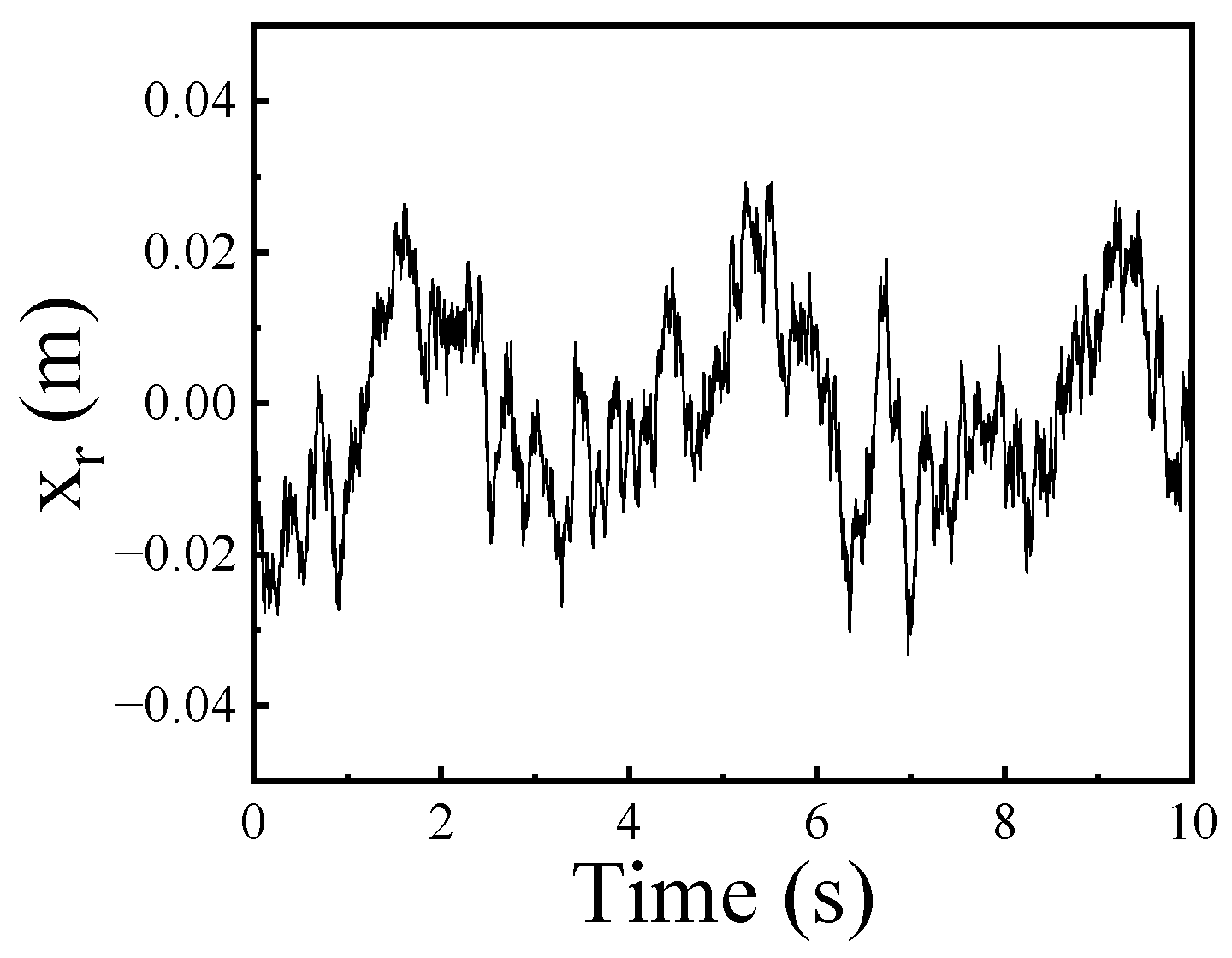
Moreover, the wavenumber, Ω   r a d / m , is defined from 0.0628   r a d / m   to 62.83   r a d / m , as represented in Equation (8). Figure 2 illustrates the road excitation applied to the quarter car model.
Δ Ω = 62.83 0.0628 n 1

3. Design of Adaptive Controller

In this work, three controllers—direct and indirect adaptive sliding mode controllers (DASME, IASME) and a proportional–integral–derivative (PID) controller—are applied to compare the control performance for both a conventional vehicle and an in-wheel motor vehicle, respectively. This comparison highlights the impact of a large unsprung mass on the vibration control, ride comfort, and road holding properties of two different vehicles.

Adaptive Sliding Mode Controller and PID Controller

It is known that sliding mode control can be applied to a wide range of dynamic systems, including nonlinear systems. This controller is well established and has been adapted for various applications, such as robust control and adaptive control [4]. To derive the control force, the tracking error, e R , and the sliding surface (line), σ R , are defined as in Equations (9) and (10).
e   x d x s
σ   λ e + e ˙
The adaptive sliding mode control force, F c R , is defined as in Equation (11).
F c = Z T θ ^ + k σ + η S a t σ ϕ
where Z R 1 × 3 is a known function consisting of the desired states and measured states, as described in Equation (12); θ ^ R 3 × 1 is the estimated parameter vector, as in Equations (13) and (14). k R and η R determine the error convergence rate. ϕ R is the error boundary layer. ϕ can also be time-varying, but it is defined as a constant value in this research for simplicity.
Z = x ¨ d + λ e ˙ x ˙ s x ˙ u x s x u T
θ = m s c s k s T
θ ^ = m s ^ c s ^ k s ^ T
Accordingly, the parameter estimation error vector, θ ~ , is defined as in Equation (15) and the adaptation law is defined as in Equation (16):
θ ~ θ ^ θ
θ ^ ˙ = Γ Z T σ
To prevent excessive parameter updates, additional constraints for the adaptation law are defined, as described in Equation (17), where θ m i n and θ m a x replace each vector element with its minimum and maximum values from the θ vector, respectively. Furthermore, the parameters are projected onto a valid parameter space to ensure that they remain within the uncertainty range.
θ ^ ˙ = Γ Z T σ θ m i n θ θ m a x θ ^ < θ m i n   , θ ^ ˙ > 0   θ ^ > θ m a x ,   θ ^ ˙ < 0 0                           o t h e r w i s e              
where the symmetric matric, Γ R 3 × 3 , is defined as in Equation (22) with the adaptive rate, γ R , and weighting matrix, W R 3 × 3 , as in Equations (23) and (24).
The adaptation rate matrix, Γ , plays a crucial role in the transient control performance. Typically, the parameter values are established through a time-consuming and laborious trial-and-error process. Moreover, the lack of analytical methods and/or criteria for the determination of the adaptation rate matrix can lead to misleading comparisons of the results. Hence, auto-tuning methods for the adaptation matrix have been employed based on the following assumptions: (i) the errors remain within predefined error boundary layers; (ii) Z Z d ,   w h e r e   Z d Z x s = x d ; and (iii) Z d varies slowly. In order to derive the auto-tuned adaptation rate matrix, Equation (16) is expanded into Equation (18).
θ ^ t θ ^ 0 = 0 t Γ Z T σ   d τ
Under the given assumptions, (ii, iii), Equation (18) is further approximated as Equation (19).
θ ^ t θ ^ 0 + Γ Z d T 0 t σ   d τ
Applying the designed control force, the error dynamics, defined by Equation (10), can be expressed as in Equation (20), considering assumption (i).
m s σ ˙ + k + η ϕ σ + Z T θ ^ = Z T θ  
σ ˙ + k e q m s σ + Z d T Γ T Z d m s 0 t σ   d τ = 1 m s Z T θ Z d T θ ^ 0
By differentiating Equation (21), the error dynamic equation can be interpreted as that of a second-order system. Consequently, the adaptive rate matrix is determined in a manner similar to the design of the response of a second-order system, as described in Equations (22)–(24).
Γ   γ W 2
W = d i a g m s ¯ c s ¯ k s ¯
γ = k e q 2 4 m a x m s ξ 2 s u p Z x s = x d W 2 Z x s = x d T ,   w h e r e   k e q k + η ϕ
It is crucial to note that the derived control force does not rely on the exact true parameter values of the system. Instead, it utilizes mean values encompassing possible variations in uncertain parameters.
Subsequently, the error convergence is proven as follows: a positive definite scalar Lyapunov candidate function, V R , is defined as in Equation (25).
V   1 2 m s σ 2 + 1 2 θ ~ T Γ 1 θ ~
Since the sprung mass, m s , is a positive scalar and Γ is positive definite (the inverse is also positive definite), V can be represented as another positive definite matrix as in Equation (26).
V = 1 2 σ θ ~ T m s 0 0 Γ 1 σ θ ~
Notice that V is lower-bounded by the minimum eigenvalue of the concatenated matrix. Given that the adaptive law is formulated as in Equation (16) and Γ is symmetric, the time derivative of the Lyapunov candidate function is described as in Equation (27).
      d d t V V ˙ =   m s σ σ ˙ + θ ^ ˙ T Γ 1 θ ~                                     =   Z θ ~ σ k σ 2 η σ S a t σ ϕ + θ ^ ˙ T Γ 1 θ ~                                     =   k σ 2 η σ S a t σ ϕ                                       k σ 2
Thus, V ˙ is negative definite function and it implies that V t V t 0   t > t 0 . Consequently, V t is bounded (therefore, so are σ and θ ~ ) [27]. V ˙ is a differentiable function; in other words, t   t 1   t ,   t 2 such that V ˙ t 2 V ˙ t = V ¨ t 1 t 2 t . It is important to note that V ¨ is also bounded, as described in Equation (28), because it is a function of σ and θ ~ , which are bounded.
V ¨ σ σ ˙ = 1 m s Z θ ~ σ k σ 2 η σ S a t σ ϕ
Then, ε > 0 ,   δ > 0 such that t 2 t < δ     V ˙ t 2 V ˙ t < ϵ ,   t . In other words, they are uniformly continuous. Since V is a differentiable function that has a finite limit as t   and V ˙ is uniformly continuous, V ˙ 0 as t by Barbalat’s Lemma [28]. This implies that σ 0 as t ; therefore, the error converges.
Additionally, an indirect adaptive sliding mode controller is designed to explore the differences between the direct and indirect adaptive control approaches. The direct adaptive sliding mode controller is designed solely with the aim of error convergence, as demonstrated in its proof (hence, it does not guarantee parameter convergence). Moreover, for the parameters to converge to their true values, the “persistent excitation” condition needs to be satisfied [29]. On the other hand, indirect adaptive control separates the parameter estimation process from the error convergence control. In this research, a recursive least squares algorithm with a forgetting factor and covariance resetting approach is employed for the parameter estimation process of the indirect adaptive sliding mode controller. The recursive least squares (RLS) method is particularly useful for real-time control, where measurement data are accumulated sequentially. This method updates the parameter vector based on newly measured data, aiming to minimize the overall squared error in each correction step. To estimate the parameters, the measured sprung mass acceleration is utilized as the true value and compared with the estimated acceleration data calculated based on the quarter car model, as in Equation (29).
x ¨ s = 1 m s c s a b c o s θ s 2 x ˙ s x ˙ u k s a b c o s θ s 2 x s x u + F c o s θ s m s g       = ϖ T ϑ g w h e r e       ϖ = F c o s θ s a b c o s θ s 2 x ˙ s x ˙ u a b c o s θ s 2 x s x u T ϑ = 1 / m s c s / m s k s / m s T
The cost function for RLS that needs to be minimized is defined as in Equation (30), where α is a forgetting factor.
J ϑ = i = 1 N t α N t i ϖ T ϑ ^ x ¨ s 2
Consequently, Equation (31) is derived by solving for ϑ ^ to minimize J ϑ .
ϑ ^ t = i = 1 N t α N t i ϖ i ϖ i T 1 i = 1 N t α N t i x ¨ s i ϖ i ,         Λ t   i = 1 N t α N t i ϖ i ϖ i T 1
By expanding Equation (31) and rearranging it into a recursive form, Equation (32) is derived.
ϑ ^ t = ϑ ^ t 1 + Λ t 1 ϖ t α + ϖ t T Λ t 1 ϖ t x ¨ s t ϖ t T ϑ ^ t 1 ,   Λ t = 1 α Λ t 1 Λ t 1 ϖ t ϖ t T Λ t 1 α + ϖ t T Λ t 1 ϖ t
The implementation of a sliding mode controller necessitates access to full state values. However, in practical scenarios, measuring all state values in real time poses challenges. Specifically, obtaining measurements for the displacement and velocity may not always be feasible in many cases. Therefore, many researchers and engineers resort to acceleration measurements, which are relatively well established. To derive the displacement and velocity from these measurements, integration serves as a straightforward method. However, due to the discrete nature of sensing and unavoidable noise, integrated results often exhibit drift. Therefore, observers are commonly utilized to estimate the required state values. In this study, a Kalman filter is devised to estimate the state values based on the measured accelerations. The Kalman filter, an adaptive filter, recursively corrects the estimated values by minimizing the weighted linear least square errors, leveraging both the dynamic model and measured state values. This approach is akin to the recursive least squares (RLS) method. However, the key distinction lies in the fact that the Kalman filter incorporates statistical properties into its estimation process, whereas RLS does not consider this information. Additionally, the dynamic model implemented within the Kalman filter enables the estimation of the model states, essentially functioning as an observer [30]. To implement the Kalman filter, an estimated state vector, x R 4 , is defined as in Equation (33).
x   x 1 x 2 x 3 x 4 T
where x 1 x ^ s , x 2 x ^ u , x 3 x ^ ˙ s , and x 4 x ^ ˙ u . Now, the vehicle dynamics is modeled as a linear autonomous system. Equation (34) represents the state-space model of the quarter car model.
x ˙ = A x + B F + G x r
where A = 0 0 1 0 0 0 0 1 k s a b c o s θ s t r u t 2 m s k s a b c o s θ s t r u t 2 m s c s a b c o s θ s t r u t 2 m s c s a b c o s θ s t r u t 2 m s k s a b c o s θ s t r u t 2 m u k s a b c o s θ s t r u t 2 + k t m u c s a b c o s θ s t r u t 2 m u c s a b c o s θ s t r u t 2 m u , B = 0 0 c o s θ s t r u t m s c o s θ s t r u t m u ,
G = 0 0 0 k t m u
To discretize the system, discretization matrices are defined as in Equation (35), where subscript “ t ” represents the matrix at time “ t ”:
A t I + A Δ t ,     B t B Δ t ,     G t G Δ t
Two accelerometers are installed to measure the states. One is attached to the sprung mass, and the other one is attached to the unsprung mass. The sensor output vector, y R 2 , is defined as in Equation (36).
y   x ˙ 3 x ˙ 4 T
Using the dynamic model, the predicted measured states can be expressed as shown in Equation (37).
y ^ = C ¯ x ^ + D ¯ F + H ¯ μ r w h e r e ,     C ¯ = k s ¯ a b c o s θ s 0 2 m s ¯ k s ¯ a b c o s θ s 0 2 m s ¯ c s ¯ a b c o s θ s 0 2 m s ¯ c s ¯ a b c o s θ s 0 2 m s ¯ k s ¯ a b c o s θ s 0 2 m u k s ¯ a b c o s θ s 0 2 + k t m u c s ¯ a b c o s θ s 0 2 m u c s ¯ a b c o s θ s 0 2 m u D ¯ = c o s θ s 0 m s ¯ c o s θ s 0 m u ,   H ¯ = 0 k t m u
Notice that the system parameter matrix is also unknown. Therefore, the parameter values in the matrix are replaced by the mean value of each parameter and then the modified matrices are denoted with a bar over the value.
It is assumed that the measurement always contains Gaussian noise, and there is also a certain level of process noise in the closed-loop system. The matrix “ R ” represent a measurement noise covariance matrix, while “ Q ” denotes the process noise covariance, and they are given as follows:
R = σ 11 2 0 0 σ 22 2
Q = σ r 2
These matrices are adjusted for the discrete system, as shown in Equations (40) and (41) [31].
R t = R / Δ t
Q t = Q Δ t
To estimate the states, the Kalman gain is defined as in Equation (42) and the states are predicted based on the measurement according to Equation (43).
K t = P t t 1 C T C P t t 1 C T + R t 1
x ^ t = x ^ t t 1 + K t y t y ^ t
Once the states are predicted, the error covariance matrix is updated at time “ t ” as described in Equation (44), and then a prediction is generated for time “ t + 1 ” based on the information acquired at time “ t ”, as in Equation (45).
P t = I K t C P t t 1
P t + 1 t = A t P t A t T + G t Q t G t T
This process, from Equation (38) to Equation (41), is repeated for each sampling instance.
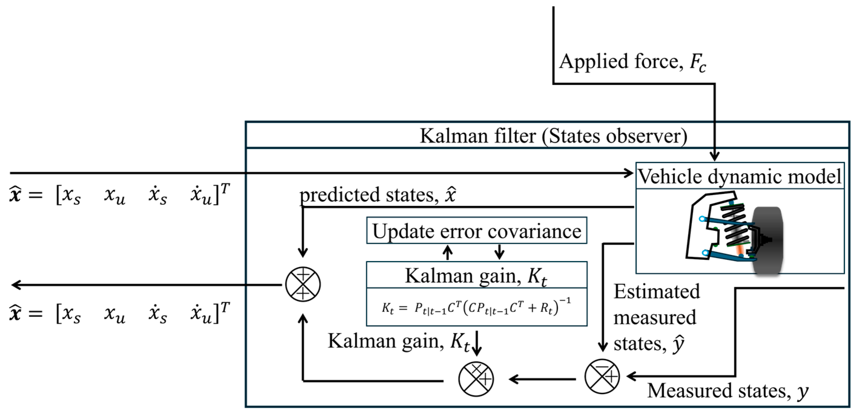
Figure 3 illustrates the integration of the adaptive sliding mode controllers and Kalman filter (observer). The objective of the closed-loop system is to isolate the vibration of the sprung mass, and thus the desired state is defined as the equilibrium point of the sprung mass. The error is calculated as the difference between the desired state and the estimated displacement of the sprung mass. This defined error, along with the estimated states and desired stated, is fed into both the controller and the adaptation law, resulting in the generation of the control input, u . It is noted that the response delay of the actuator has a critical influence on the control performance [3]. Therefore, the actuator delay is taken into account based on the assumption that the actuator exhibits a first-order system response delay. Vehicle states are measured using two accelerometers, one on the sprung mass and the other on the unsprung mass. Subsequently, the Kalman observer estimates the vehicle states based on the two measured acceleration values and the applied force. Figure 4 shows the details regarding how the direct and indirect adaptive sliding mode controllers are implemented. It is noteworthy that the adaptation law for the direct method considers the error dynamics, while the indirect method is independent of the computation of the control input. Figure 5 describes the details regarding how the Kalman observer is implemented. The applied force and estimated states are fed to the vehicle model to estimate the acceleration and other states. These estimated values are then compared with the actual measurements, followed by multiplication with the Kalman gain. This adjustment allows the estimated state values to be refined further. Finally, the key distinction among the closed-loop system and the PID controller lies in the controller part, where the control input, u, is replaced by the following equation.
u = k p e + k i e   d t + k d e ˙

4. Results and Discussion

The simulation is conducted with a sampling frequency of 2   k H z .   Commercially available accelerometers for noise, vibration, and harshness (NVH) are utilized in the simulation. Table 1 displays the specifications of the applied accelerometers. The actuator response time ranges from 1   m s for an ultra-fast MR damper to 20   m s   for a regular MR damper [4]. In this study, a commercially available MR damper with a response time of 20   m s is applied for the simulation. The actuator is modeled as a first-order system with a maximum controllable damping force of 1000   N . In-wheel motor vehicles tend to have a heavier unsprung mass due to the weight of the motor [32]. The plant parameters are defined as in Table 2. The simulations are conducted with the vehicle driving on an ISO 8608 Class C (average) road at a driving velocity of 75 k m / h to reflect the real environment.
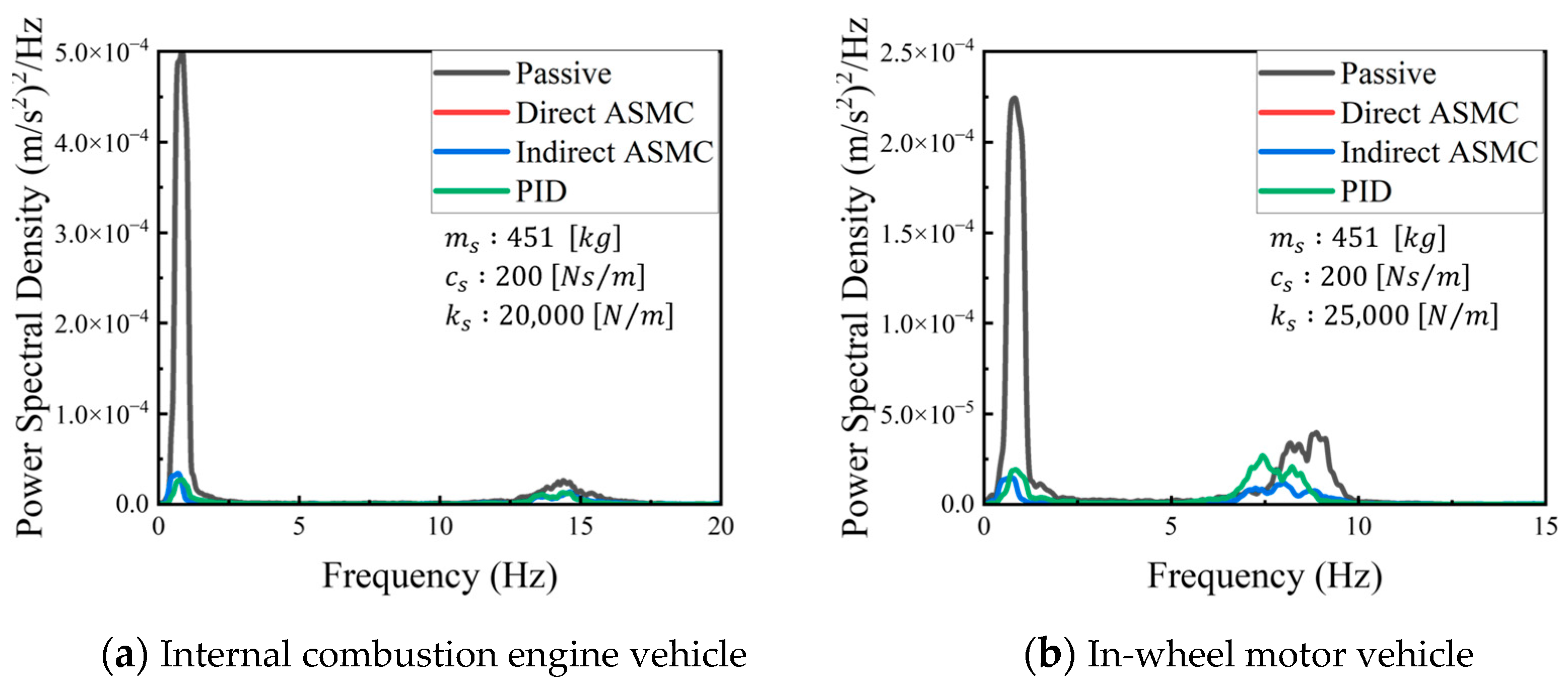
The controller gains for each controller are defined as depicted in Table 2. These gains are adjusted to achieve comparable control performance when the three controllers are applied to conventional vehicles without uncertainty, as illustrated in Figure 6a. It should be noted here that one of the goals of this work is to demonstrate the adaptability and robustness of the control algorithm and to emphasize the necessity of a control algorithm designed specifically for in-wheel drive motor vehicles. In this context, the PID gains are tuned to achieve similar vibration isolation performance to adaptive control algorithms when applied to a conventional internal combustion engine vehicle without uncertainty (as shown in Figure 6a). Subsequently, these controllers are applied to an in-wheel vehicle with uncertainty, illustrating how the performance varies and underscoring the importance of adaptive controllers.
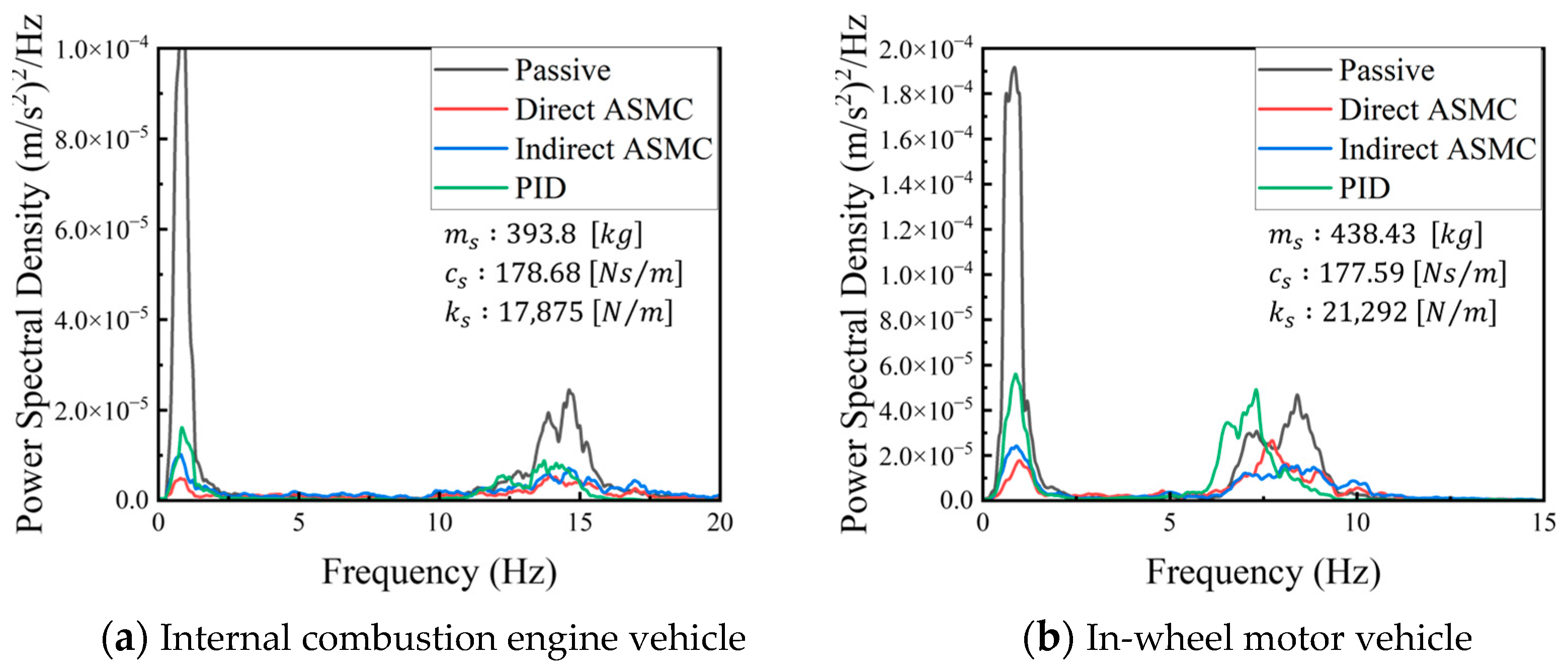
It is noted that the performance of both the indirect and direct adaptive sliding mode controllers is identical because their only difference, the adaptation law, is not implemented in the case without uncertainty. Subsequently, the robustness of each controller is investigated by applying the three controllers to suspension systems with uncertainty. The comparison of the vibration isolation performance for both types of vehicles equipped with passive dampers can be seen in Figure 6a,b. The first resonance peak, typically around 1 to 2 Hz, is closely linked to the ride comfort. Excessive vibration in this frequency range can cause discomfort among the occupants. Conversely, the second resonance peak, around 8 to 10 Hz, is related to the resonance of the unsprung mass and is critical for road holding. In-wheel motor vehicles, with their heavier unsprung mass and the resulting higher tire stiffness, face challenges in vibration control compared to combustion engine vehicles. It is important to note that passive dampers exhibit higher vibration levels for in-wheel motor vehicles compared to internal combustion engine vehicles due to the inherent system characteristics. Furthermore, the power spectral density of the acceleration shows notable differences, particularly in the resonance frequency of the unsprung mass. While the resonance frequency of the sprung mass remains around 1 to 2 Hz for both vehicle types, the resonance frequencies of the unsprung mass differ. Specifically, the unsprung mass resonance of in-wheel motor vehicles is located at 7 to 10 Hz, whereas that of conventional vehicles is located at 14 Hz. As depicted in Figure 6a, the three controllers effectively reduce the vehicle vibrations compared to the passive damper case, demonstrating significant vibration reductions for both the sprung mass resonance and unsprung mass resonance. However, Figure 6b suggests some performance differences for in-wheel motor vehicles, highlighting the importance of the control algorithm. In Figure 6b and Figure 7b, both controllers show noticeable vibration reductions for the sprung mass resonance in in-wheel motor vehicles. However, they exhibit less effective vibration reduction around the resonance frequency of the unsprung mass. Figure 7a also illustrates the difference in the control performance between the two adaptive sliding mode controllers: the direct and indirect adaptation methods. Although the indirect adaptation method guarantees parameter convergence, the direct adaptive sliding mode controller shows slightly superior results. This is because the direct method provides a greater control force against system uncertainties. To assess the robustness of the proposed adaptive controllers, Figure 7b presents the control performance for the in-wheel motor cases.
The adaptive sliding mode controller demonstrates consistent control results regardless of the parameter (or system) variations, whereas the PID controller’s performance notably varies with the parameter (or system) changes. To achieve optimal performance with the PID controller, the PID gains need to be adjusted for each different system (or parameter set). This includes situations wherein the number of passengers changes, a common occurrence in real-world scenarios. Therefore, the adaptive controller offers more reliable control performance when the system faces uncertainty with a limited actuator force. The adaptive sliding mode control algorithm comprises multiple parameters that influence the control performance: the sliding slope, λ ; the nonlinear convergence parameter, η ; and the linear convergence parameter, k . However, for simplicity, all three parameters are set to identical values. For example, a gain of 1 denotes a sliding line slope of 1, a convergence rate of 1, and a linear convergence rate of 1. Like many other controllers, the control performance of adaptive sliding mode controllers depends on the chosen gain setup. In Figure 6 and Figure 7, it is demonstrated that, in terms of the vehicle dynamics, the motion of the sprung mass (the body of the vehicle) is influenced by various factors, such as road irregularities, the suspension characteristics, and the driver inputs. This motion can be complex and may not always follow a smooth, continuous function. While the acceleration data may not be perfectly continuous, they still provide valuable information about the dynamic behavior of the vehicle, since the resonances of the displacement and acceleration share the same frequency (albeit with different magnitudes—for example, the magnitude of acceleration is also a function of the frequency in simple sinusoidal motion). By analyzing the frequency content of the acceleration signal, engineers can gain insights into the frequencies at which the vehicle exhibits significant motion or vibration, which can then be correlated with subjective evaluations of the ride comfort.
Figure 8a illustrates the variation in the control performance depending on the gain setup. The graph indicates that controlling the second resonance peak is more challenging than controlling the first resonance peak. This difficulty arises from the nature of semi-active suspension control, where controlling the sprung mass force relies on the inertia force of the unsprung mass. Therefore, the exerted control force for the isolation of the sprung mass inevitably disturbs the unsprung mass, causing it to resonate more. Figure 8a also demonstrates that the vibration isolation performance for both peaks improves as the gain values increase until they reach certain values, but excessively high gains can deteriorate the control performance. Thus, selecting the appropriate gain values is crucial, and this will be a focus of our future work. In Figure 8b, the influence of the mass ratio between the unsprung mass and the sprung mass, μ = m u / m s , on the control performance is described. Multiple cases with different unsprung and sprung mass ratios are explored, while the total sum of the unsprung mass and sprung mass is held constant at 550 kg (e.g., “ μ = 50 / 500 ” represents the case with 50 kg of unsprung mass and 500 kg of sprung mass). It is crucial to note that the unsprung resonance, represented by the second peak, is significantly affected by the variation in the mass ratio, while the sprung mass resonance, represented by the first peak, is scarcely affected by this variation. Furthermore, the control performance deteriorates with a heavier unsprung mass, while that of the sprung mass is scarcely affected. Hence, to achieve optimal control performance, it is essential to adjust the control gains primarily based on suppressing the sprung mass resonance. Additionally, tuning the mass ratio between the unsprung mass and the sprung mass is crucial in mitigating the second resonance, alongside the careful selection of the tire stiffness.

5. Conclusions

In this work, two adaptive sliding mode controllers (DASMC, IASMC) were designed and applied to the vibration control of the suspension system of an in-wheel motor vehicle, which had a much heavier unsprung mass than the suspension system of a traditional combustion engine vehicle. The controller was synthesized considering the parameters’ uncertainties, such as the sprung mass and suspension stiffness, to guarantee control robustness associated with ride comfort and the road holding properties. To ensure practical feasibility, only two accelerometers (one for the sprung mass and the other for the unsprung mass) were adopted, and the rest of the state values were estimated using a Kalman observer. In this process, the sampling frequency of the feedback system and the specifications of the accelerometers, such as the resolution, were considered to ensure accurate simulation results. Subsequently, the designed controller was applied to a quarter car suspension model, which represented the suspension systems of both the in-wheel motor vehicle and combustion engine vehicle, by choosing different parameters, especially focusing on the unsprung mass. The results achieved from the computer simulations based on a vehicle driving on an ISO 8608 Class C (average) road at 75 km/h are summarized as follows.
(1)
It has been shown that the power spectral density of the acceleration shows notable differences between combustion engine vehicles and in-wheel motor vehicles, particularly in the resonance frequency of the wheel mode. While the resonance frequency of the body mode remains around 1 to 2 Hz for both vehicle types, the resonance frequency of the unsprung mass is from 12 to 13 Hz for the combustion engine vehicle and from 7 to 10 Hz for the in-wheel motor vehicle. Therefore, the reduction of the second peak (wheel mode) is significant in the suspension systems of electric vehicles.
(2)
It has been identified that the proposed ASMCs can greatly reduce unwanted vibrations for the first and second resonant frequencies in the presence of parameter uncertainties. The vibration reduction (or power spectral density) was identified as 70% and 50% for the first mode and second mode, respectively, compared to the PID controller.
(3)
It has been demonstrated that with a higher gain of the ASMCs, better vibration control performance is achieved at both modes. However, the control evaluation with respect to the ratio of the unsprung mass over the sprung mass shows irregular vibration control performance at the second mode’s natural frequency. The second mode’s natural frequency and the peak value are changed at different mass ratios, in a non-deterministic manner. Therefore, controlling the second resonance peak is more challenging than controlling the first resonance peak. In other words, the control of road holding (steering stability) is more difficult than the control of the ride comfort in an in-wheel motor vehicle, even if a robust adaptive controller has been used.
It is finally remarked that the selection of the optimization ratio between the sprung and unsprung masses, the development of an adaptive controller integrated with an optimal controller where the states and control forces can be tuned by weighting matrices, and the design of a new type of suspension system whose configuration is significantly different from the conventional suspension system will be explored in the future to achieve enhanced vibration control performance at both resonance frequencies.

Author Contributions

Conceptualization, S.-B.C.; methodology, S.-B.C.; validation, D.-S.Y.; formal analysis, S.-B.C. and D.-S.Y.; investigation, D.-S.Y.; resources, D.-S.Y.; data curation, D.-S.Y.; writing, S.-B.C. and D.-S.Y.; original draft preparation, S.-B.C. and D.-S.Y.; review and editing, S.-B.C.; visualization, D.-S.Y.; supervision, S.-B.C. All authors have read and agreed to the published version of the manuscript.

Funding

This research received no external funding.

Data Availability Statement

The data are available upon request from the authors.

Conflicts of Interest

The authors declare no conflicts of interest.

References

  1. Nie, S.; Zhuang, Y.; Wang, Y.; Guo, K. Velocity & displacement-dependent damper: A novel passive shock absorber inspired by the semi-active control. Mech. Syst. Signal Process. 2018, 99, 730–746. [Google Scholar] [CrossRef]
  2. Williams, D.E.; Haddad, W.M. Active Suspension Control to Improve Vehicle Ride and Handling. Veh. Syst. Dyn. 1997, 28, 1–24. [Google Scholar] [CrossRef]
  3. Pazooki, A.; Goodarzi, A.; Khajepour, A.; Soltani, A.; Porlier, C. A novel approach for the design and analysis of nonlinear dampers for automotive suspensions. J. Vib. Control. 2018, 24, 3132–3147. [Google Scholar] [CrossRef]
  4. Yoon, D.-S.; Kim, G.-W.; Choi, S.-B. Response time of magnetorheological dampers to current inputs in a semi-active suspension system: Modeling, control and sensitivity analysis. Mech. Syst. Signal Process. 2020, 146, 106999. [Google Scholar] [CrossRef]
  5. Atindana, V.A.; Xu, X.; Kwaku, N.J.; Akayeti, A.; Jiang, X. A novel semi-active control of an integrated chassis and seat quasi-zero stiffness suspension system for off-road vehicles. J. Vib. Control. 2024, 10775463231224835. [Google Scholar] [CrossRef]
  6. Ata, W.G.; Salem, A.M. Semi-active control of tracked vehicle suspension incorporating magnetorheological dampers. Veh. Syst. Dyn. 2017, 55, 626–647. [Google Scholar] [CrossRef]
  7. Choi, S.B.; Han, Y.M. Magnetorheological Fluid Technology: Applications in Vehicle Systems; CRC Press: Boca Raton, FL, USA, 2012. [Google Scholar]
  8. Olabi, A.; Grunwald, A. Design and application of magneto-rheological fluid. Mater. Des. 2006, 28, 2658–2664. [Google Scholar] [CrossRef]
  9. Kosuru, V.S.R.; Kavasseri Venkitaraman, A. Trends and challenges in electric vehicle motor drivelines—A review. Int. J. Electr. Comput. Eng. Syst. 2023, 14, 485–495. [Google Scholar]
  10. Hecht, C.; Spreuer, K.G.; Figgener, J.; Sauer, D.U. Market Review and Technical Properties of Electric Vehicles in Germany. Vehicles 2022, 4, 903–916. [Google Scholar] [CrossRef]
  11. Pramuanjaroenkij, A.; Kakaç, S. The fuel cell electric vehicles: The highlight review. Int. J. Hydrogen Energy 2023, 48, 9401–9425. [Google Scholar] [CrossRef]
  12. Wellings, J.; Greenwood, D.; Coles, S.R. Understanding the Future Impacts of Electric Vehicles—An Analysis of Multiple Factors That Influence the Market. Vehicles 2021, 3, 851–871. [Google Scholar] [CrossRef]
  13. Mai, V.N.; Yoon, D.-S.; Choi, S.-B.; Kim, G.-W. Explicit model predictive control of semi-active suspension systems with magneto-rheological dampers subject to input constraints. J. Intell. Mater. Syst. Struct. 2020, 31, 1157–1170. [Google Scholar] [CrossRef]
  14. Fallah, A.Y.; Taghikhany, T. Robust semi-active control for uncertain structures and smart dampers. Smart Mater. Struct. 2014, 23, 095040. [Google Scholar] [CrossRef]
  15. Zambare, H.; Khoje, A.; Patil, S.; Razban, A. MR Damper Modeling Performance Comparison Including Hysteresis and Damper Optimization. IEEE Access 2021, 9, 24560–24569. [Google Scholar] [CrossRef]
  16. Strecker, Z.; Mazůrek, I.; Roupec, J.; Klapka, M. Influence of MR damper response time on semiactive suspension control efficiency. Meccanica 2015, 50, 1949–1959. [Google Scholar] [CrossRef]
  17. Guan, X.; Guo, P.; Ou, J. Study of the response time of MR dampers. In Proceedings of the Second International Conference on Smart Materials and Nanotechnology in Engineering, Weihai, China, 8–11 July 2009; SPIE: Bellingham, WA, USA, 2009; Volume 7493, pp. 243–251. [Google Scholar]
  18. Jeniš, F.; Kubík, M.; Macháček, O.; Šebesta, K.; Strecker, Z. Insight into the response time of fail-safe magne-torheo-logical damper. Smart Mater. Struct. 2020, 30, 017004. [Google Scholar] [CrossRef]
  19. Sanguesa, J.A.; Torres-Sanz, V.; Garrido, P.; Martinez, F.J.; Marquez-Barja, J.M. A review on electric vehicles: Tech-nologies and challenges. Smart Cities 2021, 4, 372–404. [Google Scholar] [CrossRef]
  20. Van Mierlo, J.; Berecibar, M.; El Baghdadi, M.; De Cauwer, C.; Messagie, M.; Coosemans, T.; Jacobs, V.A.; Hegazy, O. Beyond the State of the Art of Electric Vehicles: A Fact-Based Paper of the Current and Prospective Electric Vehicle Technologies. World Electr. Veh. J. 2021, 12, 20. [Google Scholar] [CrossRef]
  21. Yong, J.Y.; Ramachandaramurthy, V.K.; Tan, K.M.; Mithulananthan, N. A review on the state-of-the-art technologies of electric vehicle, its impacts and prospects. Renew. Sustain. Energy Rev. 2015, 49, 365–385. [Google Scholar] [CrossRef]
  22. Zhao, Y.; Zhang, Y.; Zhao, Y. Stability control system for four-in-wheel-motor drive electric vehicle. In Proceedings of the 2009 Sixth International Conference on Fuzzy Systems and Knowledge Discovery, Tianjin, China, 14–16 August 2009; IEEE: Piscataway, NJ, USA, 2009; Volume 4, pp. 171–175. [Google Scholar]
  23. Anaya-Martinez, M.; Lozoya-Santos, J.-D.; Félix-Herrán, L.; Tudon-Martinez, J.-C.; Ramirez-Mendoza, R.-A.; Morales-Menendez, R. Control of Automotive Semi-Active MR Suspensions for In-Wheel Electric Vehicles. Appl. Sci. 2020, 10, 4522. [Google Scholar] [CrossRef]
  24. Dodds, C.J.; Robson, J.D. The description of road surface roughness. J. Sound Vib. 1973, 31, 175–183. [Google Scholar] [CrossRef]
  25. Rill, G. Road Vehicle Dynamics: Fundamentals and Modeling; CRC Press: Boca Raton, FL, USA, 2011. [Google Scholar]
  26. Technical Committee ISO/TC, Mechanical Vibration, Shock. Subcommittee SC2 Measurement, Evaluation of Mechanical Vi-bration and Shock as Applied to Machines. In Mechanical Vibration—Road Surface Profiles—Reporting of Measured Data; International Organization for Standardization: Geneva, Switzerland, 1995; Volume 8608. [Google Scholar]
  27. Slotine, J.J.E. Applied Nonlinear Control. PRENTICE-HALL Google Sch. 1991, 2, 1123–1131. [Google Scholar]
  28. Khalil, H.K. Control of Nonlinear Systems; Prentice Hall: New York, NY, USA, 2002. [Google Scholar]
  29. Fei, J.; Batur, C. Adaptive sliding mode control with sliding mode observer for a microelectromechanical vibratory gyroscope. Proc. Inst. Mech. Eng. Part I J. Syst. Control Eng. 2008, 222, 839–849. [Google Scholar] [CrossRef]
  30. Lewis, F.L.; Xie, L.; Popa, D. Optimal and Robust Estimation: With an Introduction to Stochastic Control Theory; CRC Press: Boca Raton, FL, USA, 2017. [Google Scholar]
  31. Brown, R.G.; Hwang, P.Y. Introduction to Random Signals and Applied Kalman Filtering: With MATLAB Exercises and Solutions. 1997. Available online: https://ui.adsabs.harvard.edu/abs/1997itrs.book.....B/abstract (accessed on 20 June 2024).
  32. Kim, Y.-J.; Sohn, Y.; Chang, S.; Choi, S.-B.; Oh, J.-S. Vibration Control of Car Body and Wheel Motions for In-Wheel Motor Vehicles Using Road Type Classification. Actuators 2024, 13, 80. [Google Scholar] [CrossRef]
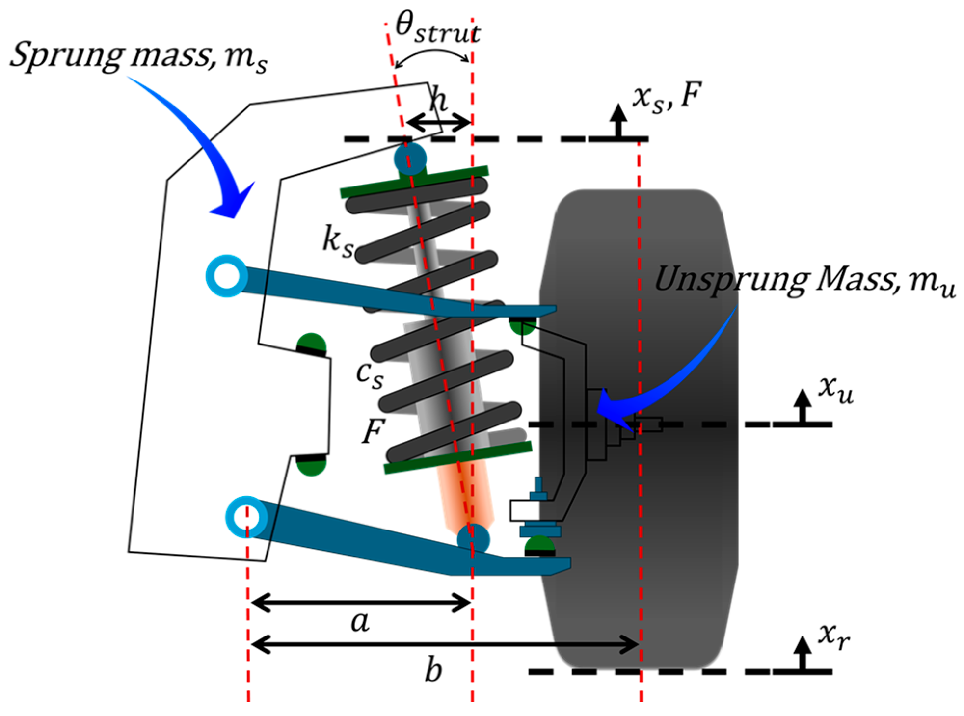
Figure 1. Quarter car model of the in-wheel motor vehicle.
Machines 12 00433 g001
Figure 2. ISO 8608 Class C random road excitation with a driving velocity of 75 k m / h .
Machines 12 00433 g002
Figure 3. Block diagram of proposed adaptive control system.
Machines 12 00433 g003
Figure 4. Block diagram of adaptive sliding mode controller: (a) direct adaptive control system, (b) indirect adaptive control system.
Machines 12 00433 g004
Figure 5. Block diagram of Kalman observer.
Machines 12 00433 g005
Figure 6. Without parameter uncertainties: (a) internal combustion engine vehicle, (b) in-wheel motor vehicle.
Machines 12 00433 g006
Figure 7. With parameter uncertainties: (a) internal combustion engine, (b) in-wheel motor vehicle.
Machines 12 00433 g007
Figure 8. Adaptive sliding mode controller performance: (a) with respect to gain choice, (b) with respect to unsprung mass and sprung mass ratio ( μ = m u / m s ).
Machines 12 00433 g008
Table 1. Accelerometer specifications.
ParameterValueUnit
Resolution2830 μ g
Measurable range ± 10 g
Noise level2000 (or 200) μ g r m s   ( or   μ g r m s / H z )
Table 2. Parameters’ symbols and values.
ParameterValueUnit
Percent uncertainty, υ ± 15 %
Average sprung mass, m s ¯ 451 k g
Average damping coefficient, c s ¯ 200 N s / m
Average suspension stiffness (conventional), k s ¯ 20,000 N / m
Average suspension stiffness (in-wheel motor), k s ¯ 25,000 N / m
Tire stiffness (conventional), k t 230,000 N / m
Tire stiffness (in-wheel motor), k t 300,190 N / m
Unsprung mass (conventional), m u 28.5 k g
Unsprung mass (in-wheel motor), m u 100.908 k g
Driving velocity75 k m / h
Strut fixture angle, θ s t r u t 27 ° ( d e g r e e )
Geometric parameters for quarter car model, a , b   a n d   h 0.19, 0.32, 0.16 m
Auto-tune rate (for adaptive control), ξ 0.707N/A
Adaptive sliding mode controller
(direct/indirect)
Sliding line slope, λ 1N/A
Convergence rate, η 1N/A
Linear convergence rate, k 1N/A
PID controllerProportional gain, k p 1000N/A
Integral gain, k i 100N/A
Derivative gain, k d 1000N/A
Disclaimer/Publisher’s Note: The statements, opinions and data contained in all publications are solely those of the individual author(s) and contributor(s) and not of MDPI and/or the editor(s). MDPI and/or the editor(s) disclaim responsibility for any injury to people or property resulting from any ideas, methods, instructions or products referred to in the content.