Abstract
Worms can be produced using special machines or standard lathes equipped with a whirling thread-cutting device. A blank is placed on the mandrel and tightened using the three-jawed chuck of the standard lathe. If the workpiece diameter is excessively large, passage through the driven pulley is not possible, and the workpiece cannot be supported. Therefore, a new tool holder for whirling devices is needed. During the whirling process, vibrations in the form of machine velocity amplitudes were measured. After whirling was complete, roughness values were calculated. Using numerical procedures of Wolfram Mathematica 10, vibration peaks were extracted, from which frequencies and maximum amplitudes were determined. The data were then inputted into Design Expert, and the rotational speed and amount of separated material were optimized. The results of the study showed that the quality of the processed surface did not improve with processing in two passes of the tool. The measured vibration amplitudes on the lathe carrier and thread whirling attachment increased with cutting speed at the same cutting depth, whereas the quality of the machined surface was best at the smallest and largest cutting depths.
1. Introduction
Threads of smaller dimensions can be made by turning, using a form tool over several passes. The production of large-dimension threads is problematic, given the large cutting surface and associated large cutting forces. In such cases, thread-cutting proceeds on standard lathes equipped with whirling thread-cutting devices that are mounted in place of the tool holder or on special whirling–cutting machine tools. Whirling technology is an efficient method for screw and worm production compared to classical methods and ensures good thread surface quality in a single pass. A blank is clamped in the lathe chuck and rotated very slowly, usually in the same direction as the cutting ring. One to four cutting tools fixed to the whirling ring rotate at high speed and are inclined around the horizontal axis at the lead angle appropriate for the thread-pitch diameter. Multiple cutting tools reduce the chip load and, therefore, the cutting forces; however, this requires more precise adjustment of the tool so that each cutting blade processes equal amounts of material.
The chip thickness increases from zero to a maximum value as the vibrations and cutting forces rise. The maximum workpiece diameter depends on both the hole size of the driven pulley and the inner-bearing diameter of the whirling attachment. During whirling, the workpiece passes through the entire length of the whirling attachment.
If the workpiece diameter is excessively large, passage through a cutting ring with a driven pulley is not possible. Thus, the tool holder used for machining must be adjusted to prevent undercutting. This removes the support but is possible in specific instances when the workpiece is not too long. It is essential to be familiar with the theory of whirling and the characteristics of the lathe and whirling attachment.
Several researchers have explored designs appropriate for worm cutting, the relevant kinematics, tool profiling, and the effects of cutting parameters. Cretu and Coteata [1] explored the effects of cutting and tool geometric parameters on the precision of worm gears manufactured via whirling thread-cutting. They reported that the thickness of a manufactured tooth depended on the precision with which the cutting depth was set, which was, in turn, affected by the precision of the lathe carrier positioning in the transverse direction. The whirling device required precise positioning using a comparator device prior to trial cutting, as well as careful definition of the tooth thickness.
Cretu [2,3], of the same group, designed whirling thread-cutting devices appropriate for ordinary lathes and showed that the quality of machined surfaces depended on both the cutting speed and feed rate. In 2017 [4], the same author systematically analyzed worm-screw manufacturing methods for whirling devices, exploring the characteristics of the machined material, the screw and tool design parameters, the features of whirling thread devices, and the shaft precision required for machining.
Merticaru et al. [5] modeled a whirling process based on geometrical and kinematical parameters that reduced surface irregularities and enhanced the precision of machined surfaces. They found that only a few parameters of the worm threading process significantly influenced the precision and microgeometry of the generated surfaces.
A whirling process modeled and simulated based on the equivalent cutting volume was presented in [6]. The model revealed that the tool-edge geometry affected the cutting forces.
Soshi et al. [7] explored the utility of whirling tools fabricated from cubic boron nitride and polycrystalline diamond (alternatives to carbide) mounted on direct motor-driven whirling units.
Lexiang et al. [8] developed a cutting-force model that facilitated the selection of cutting parameters that minimized the specific cutting energy. In turn, this enhanced manufacturing sustainability.
The vibrations of a cutter-workpiece system were analyzed in [9] in an effort to identify the characteristics of airfoil blade whirling that facilitated dynamic performance. A theoretical model was developed that considered the dynamic parameters of the workpiece and the geometric immersion of the whirling cutter to predict stability.
The processing method presented in [10] used a modified whirling device to overcome the dimensional restrictions of the screw. The standard tool holder was replaced by a novel holder with a larger cutting-circle diameter, and the roughness values of the machined pieces were measured.
Engineers commonly measure vibration in an effort to reduce vibration for improved machining and machine performance [11]. Velocity and acceleration sensors are often used to measure and monitor vibrations. Overviews of the measurement process and the analysis requirements for transport noise and vibration have been proposed [12,13]. For example, the root mean square (RMS) values can be used to calculate the vibration amplitude [14,15].
In [16], several methods were applied to calculate the maximum frequency of a spectrum. The results were mutually compared to determine the most accurate testing method for vibration-dominant frequency determination. In engineering practice, it is often necessary to determine several so-called dominant frequencies or local maxima. An algorithm for computerized multi-peak detection as a part of an intelligent fault detection system for rotary machines was also developed.
This article is a continuation of our research [10] on two-pass machining of highly machinable materials, with the aim of ensuring the best possible surface quality.
2. Whirling on a Universal Lathe
Whirling, the most productive method of manufacturing the worm, can be performed on ordinary lathes (using whirling thread-cutting devices that are mounted in place of the tool holder device) or special whirling–cutting machine tools. The high costs of the special machine tools lead to thread-cutting processes on ordinary lathes. The blank rotates relatively slowly, and it is eccentrically encircled by the tools, which rotate with a high revolution. The blank and the cutting tools rotate either in the same direction as the feeding movement (i.e., up-cutting manufacturing) or in the opposite direction (i.e., down-cutting manufacturing) when the spinning senses of the tool and the blank are conflicting. In the case of up-cutting manufacturing used in the present experiment, the chip thickness increases from the value of zero to the maximum value. This increase has a negative effect on the tool face of the cutting tool because it generates accelerated wear of this face. Thus, the cutting tool must be sharpened after each screw has been machined. Whirling machining also generates a short, thin chip that is easy to remove from the cutting area. The whirling thread-cutting methods, which utilize an inner point of contact, are most frequently utilized due to their advantages of high cutting flank precision, very small errors with respect to the ideal profile, good blade cooling, and the ability to achieve small roughness values.
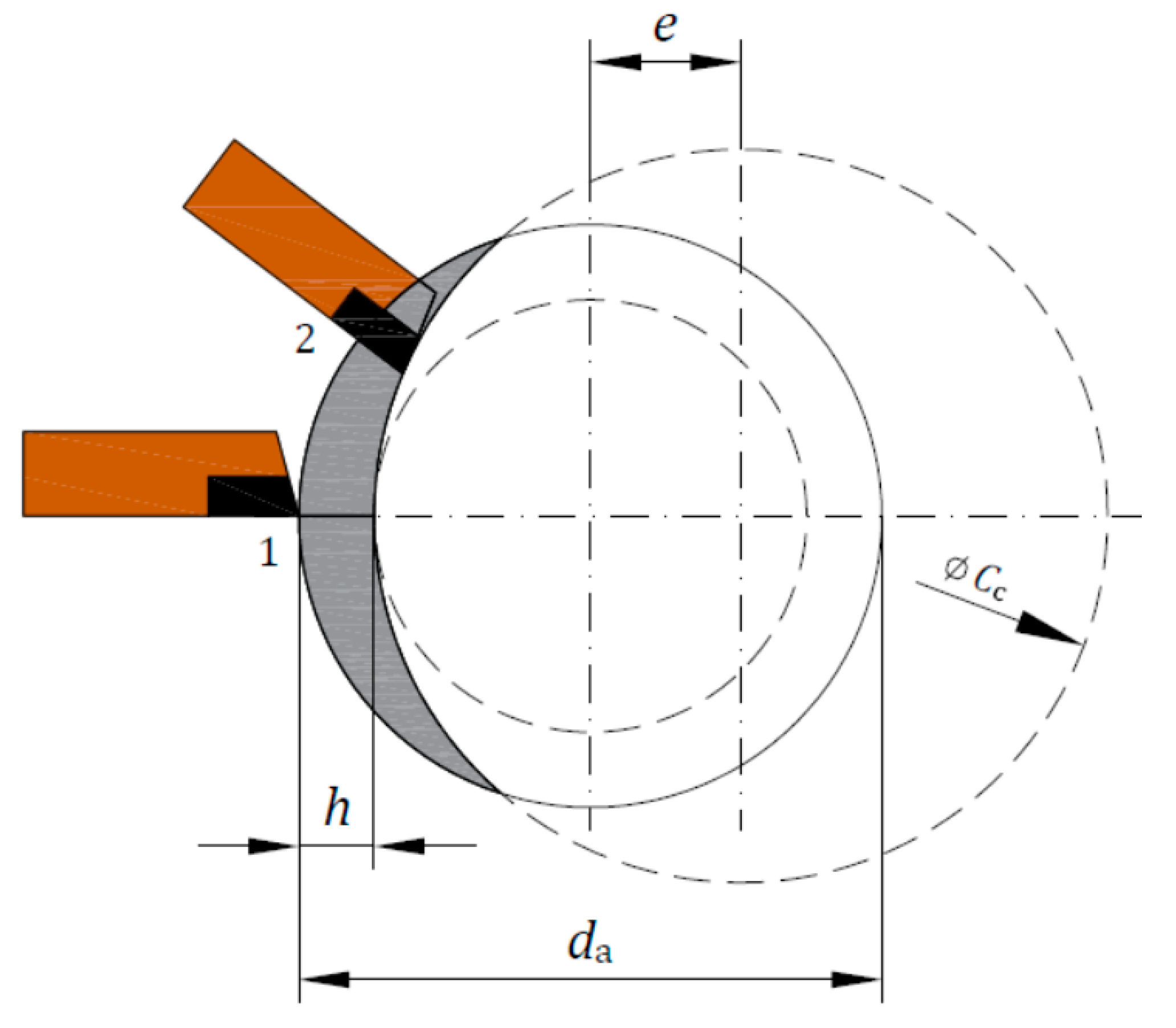
In our previous study [10], a screw for a small dry extruder used to process soybeans was made utilizing a universal lathe with a whirling attachment, and the surface quality was measured. The cutting tool was a carbide-tipped insert mounted on a specially designed cutting head of the whirling attachment. The charge on the cutting head, the rotational speeds of the tool and the workpiece, and the feed rate and cutting depth were adjusted by the required screw dimensions. As Figure 1 shows, the tool first touches the workpiece (position 1) and then moves toward the center by a distance equal to the thread height h (position 2).

Figure 1.
Geometrical position of the whirling tool.
To avoid interference between the workpiece and the inner part of the (hollow) driven pulley, the diameter of the cutting circle ϕCc must be larger than the workpiece diameter da by a factor of 1.4–1.6. If this factor is not correct, undercutting that yields an irregular screw profile will result. In the machining in this study, a cutting head with a cutting circle diameter of 1.9 da was used. The standard tool holder ring was replaced by a novel tool holder (a cutting head) that was threaded directly to the driven pulley (Figure 2).
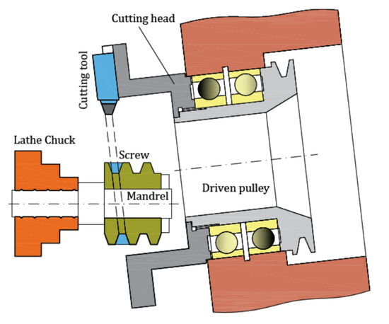
Figure 2.
Inclination of the tool head.
Thread whirling is a discontinuous process. It is important that the tool holder is rigid enough to pick up vibrations resulting from splintering. The cutting circle diameter is usually as low as possible for splintering to take place on a large circle arc, thus reducing the vibrations. To achieve a sufficiently high cutting speed and avoid interference between the cutting tool and the lathe chuck, a slightly larger cutting circle diameter was used.
It is also important that the spinning axe of the whirling cutting tool be parallel to the spinning axe of the blank. To achieve this arrangement, a dial gauge was used to adjust the height of the cutting tool ring.
The whirling attachment was inclined around the horizontal axis, and the tool rings around the vertical axis at angles equal to the screw lead angle. This reduced the number of passages through the driven pulley and also the risk of interference between the workpiece and the inner part of the pulley (Figure 2).
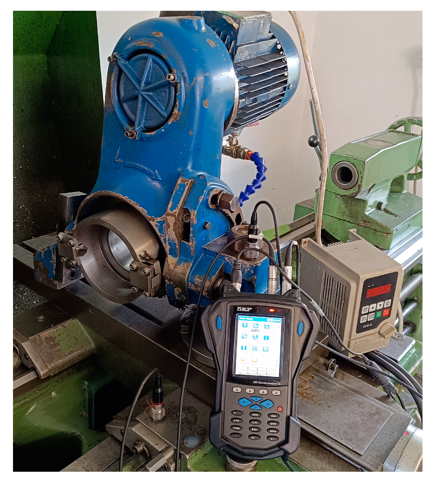
The main cutting motion of the whirling device was performed by a 1.1-kW electric motor that transmitted the rotating movement at the whirling thread-cutting device using a SPA-type V-shaped belt. Stretching of the belt was carried out via the egg-shaped holes through which the electric motor was fixed on the case of the whirling attachment. The V-belt pulley of the electric motor on the thread whirling attachment had a diameter of 94 mm. The driven pulley, mounted on the inner side of radial roller bearings along with the tool-cutting ring, had a diameter of 140 mm. Four cutting speeds were used for machining, and a frequency converter was utilized. Each blank was placed on the mandrel and tightened using the three-jawed chuck of a Böehringer lathe (Figure 3).
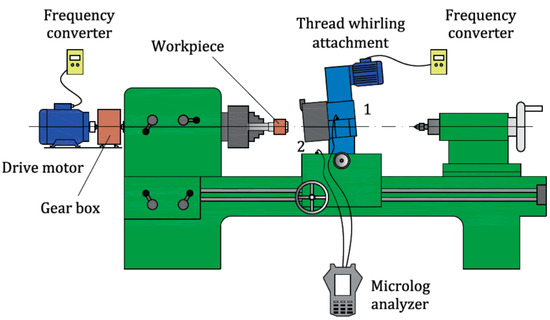
Figure 3.
Universal lathe with various accessories.
3. Experiment Setup
The thread-whirling attachment was fastened to the lathe carrier on the front side via four hexagon-socked head screws placed in the groves, which secured the compound rest to the cross slide of the lathe machine. On the back side, for fastening, two non-standard-shaped screws were placed in the groves of the cross slide. This enabled sufficiently rigid clamping of the thread whirling attachment and, thus, stable processing.
The accuracy of the transversal carrier of the lathe was 0.1 mm, which influenced the accuracy of position settling in the radial direction of the cutting tool in the whirling device. The speed of the main lathe spindle could be varied from 11.2 to 2240 rpm. Using a frequency converter, the lowest speed (11.2 rpm) was reduced by 90% (to 1.12 rpm). Further reduction was not possible due to torque loss and the cessation of main spindle rotation. The cutting tool and blank exhibited the same direction of rotation as in down-milling.
A gearbox with a 1:15 gear ratio (Figure 3) was used to reduce the workpiece rotation from 1.12 to 0.075 rpm. The main lathe motor was removed, and the lathe main spindle was operated with the aid of another drive motor using a frequency converter connected to the gearbox with simple coupling. The material removal rate was thus lowered, as was the feed rate per tool.
The cutting head rpm n2 is given by
where n1 is the rpm of the electric motor, d1 is the diameter of the driving pulley, and d2 is the diameter of the driven pulley.
The cutting speed is therefore:
where Cc is the diameter of the cutting circle.
Four cutting speeds were used by changing the rpm of the electric motor that powered the whirling attachment (Table 1).

Table 1.
Whirling cutting device parameters.
The dimensions of the screw are listed in Table 2.

Table 2.
Screw geometry.
Rather than 16MnCr5 material, 11SMn30 material was used for processing (Table 3). The latter is marked by good machinability on machine tools and by easy fragmentation of chips; thus, its machined surface was expected to be of better quality. Due to their high sulfur and phosphorus content, free-cutting steels not destined for heat treatment generally are not recommended for welding. The chemical composition of the 11SMn30 material was as follows: C max 0.14, Si max 0.05, Mn 0.9–1.3, P max 0.11, and S 0.27–0.33.

Table 3.
Mechanical properties of steel 11SMn30.
Processing was performed without any support due to the risk of interference between the driven pulley and the revolving center. The cutting tool was cooled during machining with a bonderite L-MR 72 coolant trough hollow in the driven pulley of the whirling attachment. The temperature of the tool remained low during machining; the amount of energy directed into the workpiece was also small. The generated heat was removed from the cutting area, primarily with chips and partially with coolant, because the workpiece temperature remained low during the course of machining. This allowed for the use of higher cutting speeds without the danger of exceeding the temperature resistance of the cutting tool or overheating the workpiece.
Cuts were made at a certain cutting speed to a depth of 8 mm over two passes at three cutting depths. In the first pass, the screw was processed to depths of 6, 7.2, and 7.8 mm; in the second pass, processing continued to yield the final screw dimensions (Table 4).

Table 4.
Cutting parameters.
Before the initiation of machining, vibrations were measured on the whirling attachment and the lathe carriage (Figure 3). Vibrations also were measured after the cutting tool fully entered the material, approximately 15 mm from the screw’s beginning. The vibration was reduced when machining was performed against the feed rate because the main component of the cutting force opposed the feed rate movement and assumed control of movements from the main shaft of the lathe.
To allow comparisons, two more screws were made in one pass at the lowest cutting speed (screws 13 and 14). The main shaft speed is a parameter directly related to the longitudinal feed rate of the lathe sleeve and was a constant value for the machining of all 14 screws. The productivity of machining in this case was relatively low; however, the main goal was to achieve the best possible surface quality.
The cutting tool was a carbide insert brazed on the body, which was prismatic in shape (16 mm × 16 mm) and ground into the corresponding shape (Figure 4).
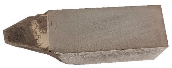
Figure 4.
Cutting tool.
The tool profile had the same profile as the hollow profile of the screw. The blade was fastened to the cutting ring with a special holder using a grove and four socked bolts (Figure 5). This allowed for easy dismantling of the tool for sharpening after the completion of screw machining.

Figure 5.
Thread whirling attachment and Microlog gx CMXA 75 analyzer.
Two tools were used for machining; when one tool was processing material, the other was sharpening. The determination of the cutting tool holder radial runout was accomplished using a dial gauge with a value of 0.05 mm. The maximum value of blank tightening on the mandrel of the three-yaw chuck was 0.03 mm.
The cutting tool was sharpened on a universal diamond grinder (granulation 100) after each tool pass. Twelve screws were fabricated using different cutting parameters, and two screws required one tool pass.
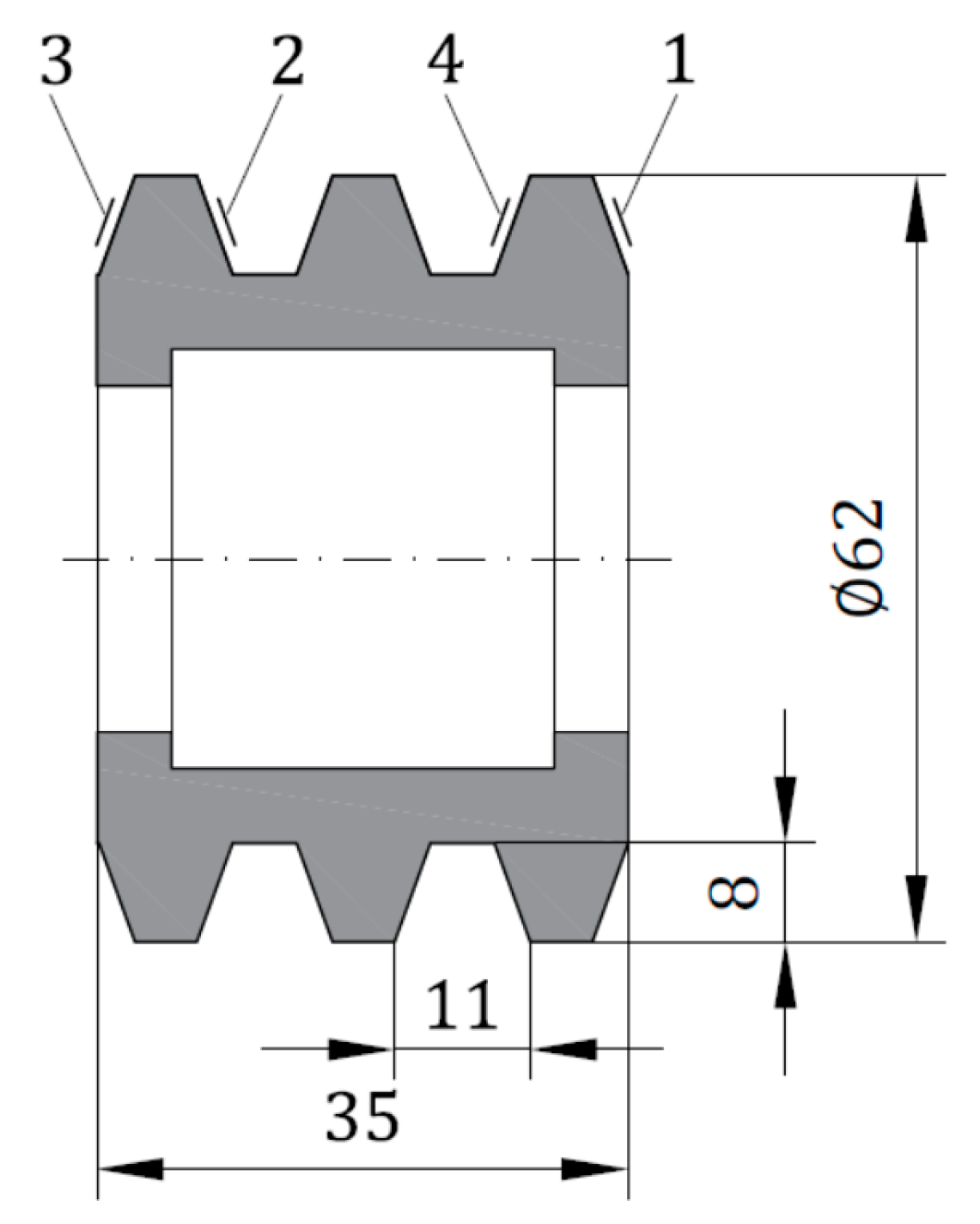
Processing quality was measured at four points (Figure 6), at the beginning and end of the screw.
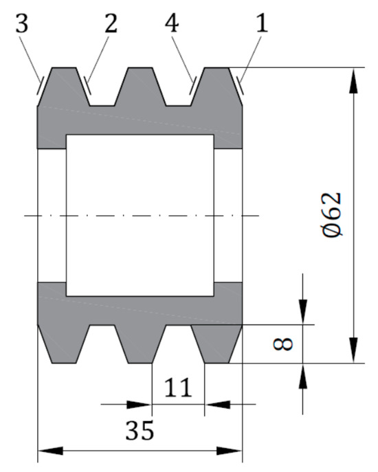
Figure 6.
Dimensions of the extruder screw and the measuring points.
Points 1 and 4 are further from, and 2 and 3 are closer to, the chuck of the lathe.
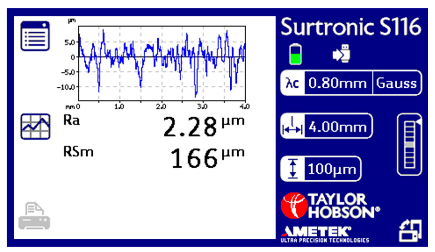
Roughness was measured using a Surtronic S-116 device (Taylor Hobson) at a screw profile length of 4 mm. The instrument can measure roughness in any orientation within 25 mm of the evaluation length. In addition to roughness data, it is possible to measure waviness parameters, parameters on the raw profile, and parameters obtained by double filtering. The instrument resolution and reading accuracy are 0.01 μm and 2%, respectively. Before the measurement, the instrument was calibrated using a reference specimen type 112/534 with 6.0 μm roughness. An example of the measurement is shown in Figure 7. A Gaussian filter was used for the measurement.

Figure 7.
Graphical representation of the roughness on the instrument.
The arithmetical mean height (Ra) and the mean width of the profile elements (Rsm) were also measured. To ensure the right position (height) between the measuring device and the screw surface, a special device that allowed the measurement of all screws in the same place was constructed, depending on the keyway of the screw.
During machining, CMSS 2200 vibration acceleration sensors were placed in two locations, as shown in Figure 3, and the data were logged by an SKF Microlog gx CMXA 75 analyzer. The sensors are designed for exceptionally low noise levels for low frequencies in the temperature range of −50 °C to 120 °C, with a sensitivity of 100 mV/g and precision of ±5%.
Initially, the maximum amplitude was extracted from each vibration profile as proposed in the literature [16]. After further consideration, the RMS value was chosen as a better representation of the total energy of the vibration profile.
The RMS value of a set of vibration amplitudes is the square root of the arithmetic mean of the squares of the values of amplitudes, also known as the quadratic mean of the amplitude.
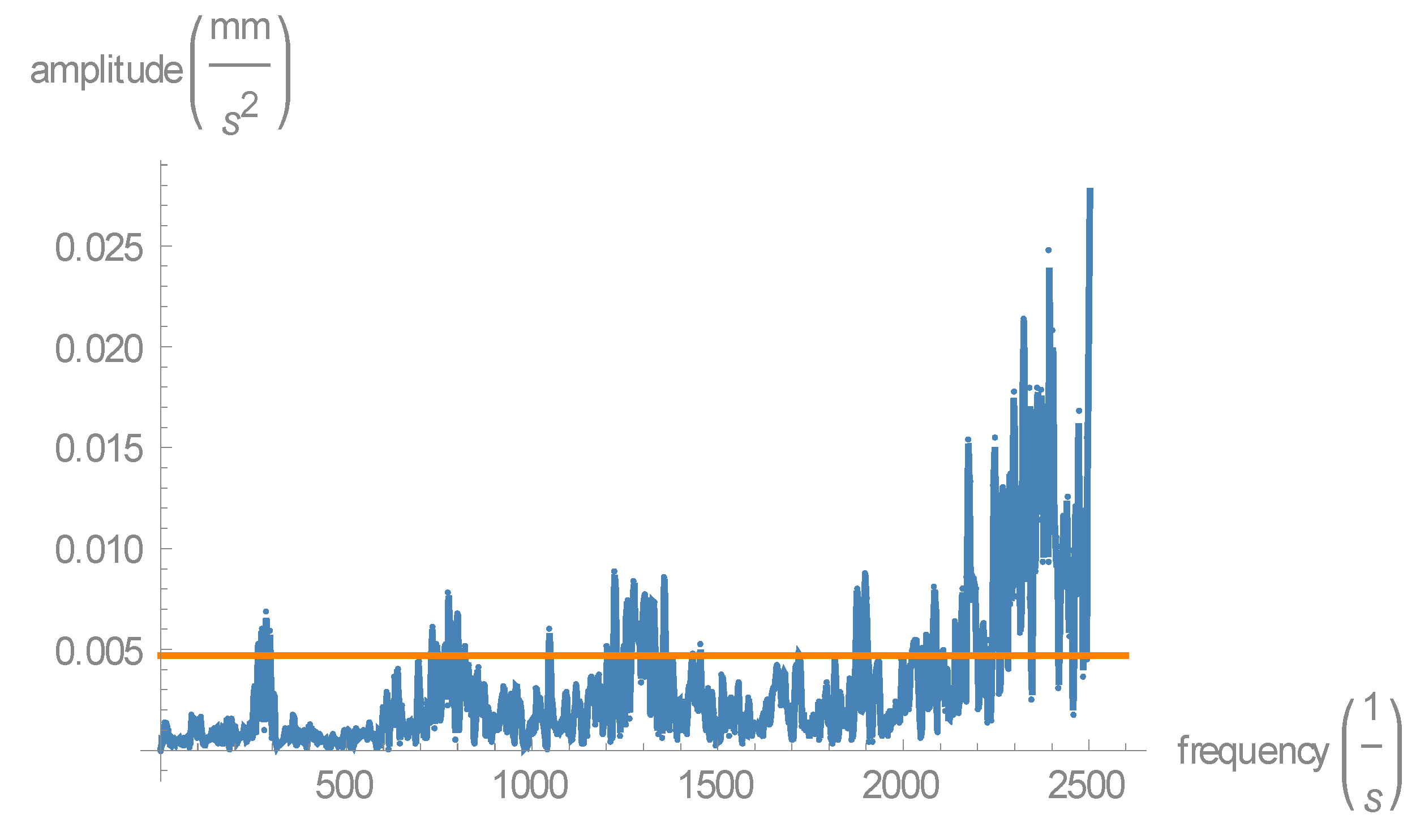
The blue lines in Figure 8 represent the amplitude at each frequency of vibration as a multiplier of g, gravitational acceleration, and the orange line is the RMS value for this dataset. This figure is a graphical representation of one set of data from which the RMS value was calculated. This type of data set was obtained for each set of input parameters from which the RMS value was extracted.
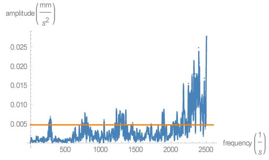
Figure 8.
Root mean square value of one set of vibration measurement data.
4. Results and Discussion
The roughness measurements are shown in Table 5. The lowest surface roughness parameter Ra was reached at points 2 and 3 (Figure 6), as expected, considering that these points are closer to the lathe chuck. Considering the cutting parameters, the lowest average surface roughness parameter, Ra, was reached at a cutting speed of 322.73 m/min and a depth of cut of 0.2 mm, although the vibration amplitudes (Table 6) were not the lowest values.

Table 5.
Surface quality.

Table 6.
Root mean square values of the vibration amplitudes.
The accuracy of the worm and the nut steering of the lathe on which the thread whirling attachment is mounted influence the accuracy of the worm thread surface, primarily with respect to the screw pitch. In this study, the primary goal was the achievement of better surface quality; deviations in screw pitch and helix profile error were not determined. Notably, this information is unimportant for screw functionality; the small length of the screw also ensured that this error was negligible.
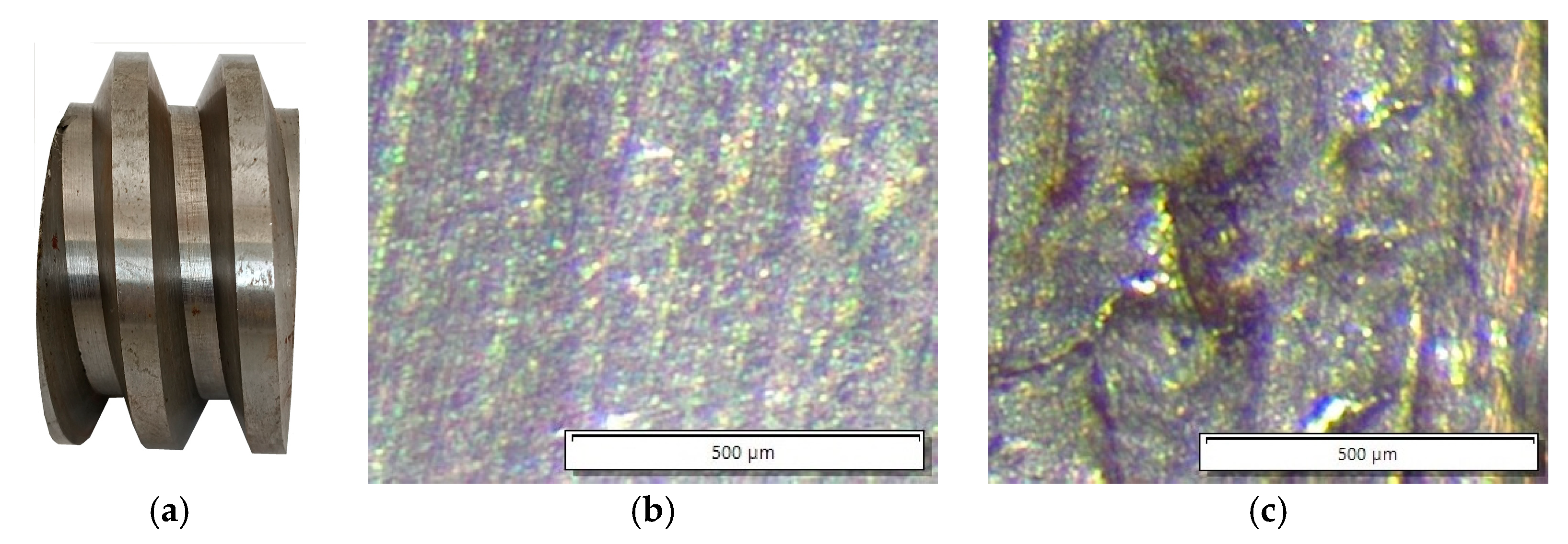
The machined surface was observed using a stereo microscope Olympus SZX 10, with two apochromatic objective lenses (Figure 9b). The surface of the screw made by whirling had a much lower roughness compared with the screw made by turning (Figure 9c).

Figure 9.
Comparison of surface quality of (a) a machined screw, (b) the surface of a screw made by whirling, and (c) the surface of a screw made by turning.
Deviation of the lateral cutting face angle depends on the correct shape of all cutting edges of the cutting tool, as well as the correct disposal of the whirling device on the lathe carriage. When sharpening the cutting tool, the inclination angles of the body of the sharpening device must be very accurate. At the time of grinding, the cutting tool was clamped in a two-axis machine vice; thus, the correct shape of the cutting edges of the tool depended on the accuracy of the division scale on the machine vice.
The results of RMS amplitudes for each dataset were calculated from the measured amplitudes stored in the Microlog device and are listed in Table 6.
Wolfram Mathematica was used to analyze the experimental data.
The first part of the numerical analysis resulted in a series of RMS data in the algorithm VIBRACIJE
VIBRACIJE
vibracije[naslov_, broj_, opcija_, pod_] :=
Module[
{ naslovstr = naslov, dataXYraw, \[CapitalDelta]f, dataaX, dataaY1,
ii, duzina, tabmx, rjesenjaaa, rjesenjaaaa, rjesenjaaaaa, plot0,
plot1, plot2, fff, pozmaksf, maksimumf, maksimumf1, prikaz, rms,
iii, op = opcija, podd = pod, dataaYY1, dataaYY2, plot3, frms,
prikaz1},
dataXYraw = Import[naslovstr, "Data"][[1]][[61 ;; 861, 1 ;; 3]];
\[CapitalDelta]f = 3.125;
dataaX = dataXYraw[[All, 1]];
dataaYY1 = dataXYraw[[All, 2]];
dataaYY2 = dataXYraw[[All, 3]];
dataaY1 = Which[podd == 1, dataaYY1, podd == 2, dataaYY2];
ii = Range[Dimensions[dataaX]] // Flatten;
duzina = Dimensions[dataaX][[1]];
iii = Table[i/i, {i, 1, Dimensions[dataaX][[1]], 1}];
tabmx = Table[{dataaX[[i]], dataaY1[[i]]}, {i, duzina}];
fff = Interpolation[tabmx, InterpolationOrder -> 1];
pozmaksf[n_] :=
Position[dataaY1, RankedMax[dataaY1, n]][[1]][[1]] - 1;
maksimumf[n_] := {pozmaksf[n], \[CapitalDelta]f*pozmaksf[n],
RankedMax[dataaY1, n]};
maksimumf1[n_] := {\[CapitalDelta]f*pozmaksf[n],
RankedMax[dataaY1, n]};
rjesenjaaa = Table[maksimumf[i], {i, 1, broj}];
rjesenjaaaa = Table[maksimumf1[i], {i, 1, broj}];
rjesenjaaaaa = SortBy[rjesenjaaaa, First];
rms = RootMeanSquare[dataaY1];
frms[x_] = rms;
plot0 =
Plot[fff[x], {x, 1, \[CapitalDelta]f*duzina}, PlotRange -> All,
AxesOrigin -> {0, 0},
AxesLabel -> {frequency [s^-1], amplitude [mm/s^2]}];
plot1 = ListPlot[tabmx, PlotRange -> All, AxesOrigin -> {0, 0}];
plot2 =
ListPlot[rjesenjaaaaa, Filling -> Axis, PlotStyle -> Red,
AxesOrigin -> {0, 0}];
plot3 = Plot [frms[x], {x, 0, 2600}, PlotStyle -> Orange];
prikaz = Show[plot0, plot1, plot2];
prikaz1 = Show[plot0, plot1, plot3];
Which[op == 1, iii, op == 2, Print[prikaz], op == 3, rms, op == 4,
rjesenjaaaaa, op == 5, Print[prikaz1]]
]
From a series of RMS data matrices, rezultati and arezultati, appropriate for further analysis, were constructed as shown in the algorithm REZULTATI.
REZULTATI
RMSrez = Table[i/i, {i, 1, Dimensions[nazivi][[1]], 1}];
Do[RMSrez[[i]] = vibracije[nazivi[[i]], 1, 3, 1], {i, n}];
RMSrez = Table[vibracije[nazivi[[i]], 1, 3, 1], {i, n}]
rezultati =
Table[{pojasnjvc[[i]], pojasnjA1[[i]], RMSrez[[i]]}, {i, 1, n}]
RMSrez1 = Table[vibracije[nazivi[[i]], 1, 3, 2], {i, n}]
arezultati =
Table[{pojasnjvc[[i]], pojasnjA1[[i]], RMSrez1[[i]]}, {i, 1, n}]
To determine the functions of response surfaces or a data model, Mathematica 10 is equipped with a Fit function. Fit is also used for linear regression and least squares fit analyses. Fit is typically applied to fit combinations of functions to data, including polynomials and exponentials. As a particularly simple way to model measurement data, the Fit function minimizes the sum of squares:
Fit[data,{f1,…,fn},{x,y,…}] finds a fit a1 f1 +…+ an fn to a list of data for functions f1,…,fn of variables {x,y,…} [17]. The following algorithm (ISPIS) uses the Fit function to find the models.
ISPIS
lpr = ListPlot3D[rezultati]
Fit[rezultati, {1, x, y, x^2, x y, y^2}, {x, y}]
model1 = Fit[rezultati, { 1, x, y, x y, x^2, y^2}, {x, y}]
Show[lpr, Graphics3D[{Red, PointSize[0.02], Map[Point, rezultati]}]]
Show[Plot3D[model1, {x, 230, 400}, {y, 0, 30},
PlotStyle -> Opacity[.5], PlotRange -> {0, 0.02},
AxesLabel -> {vc, A2, RMSY1}],
Graphics3D[{Red, PointSize[0.02], Map[Point, rezultati]}]]
pr1 = ListPlot3D[arezultati]
model12 = Fit[arezultati, {1, x, y, x^2, x y, y^2, x^3, y^3}, {x, y}]
Show[pr1, Graphics3D[{Red, PointSize[0.02], Map[Point, arezultati]}]]
Show[Plot3D[model12, {x, 230, 370}, {y, 0, 30},
PlotStyle -> Opacity[.5], PlotRange -> {0, 0.005},
AxesLabel -> {vc, A2, RMSY2}],
Graphics3D[{Red, PointSize[0.02], Map[Point, arezultati]}]]
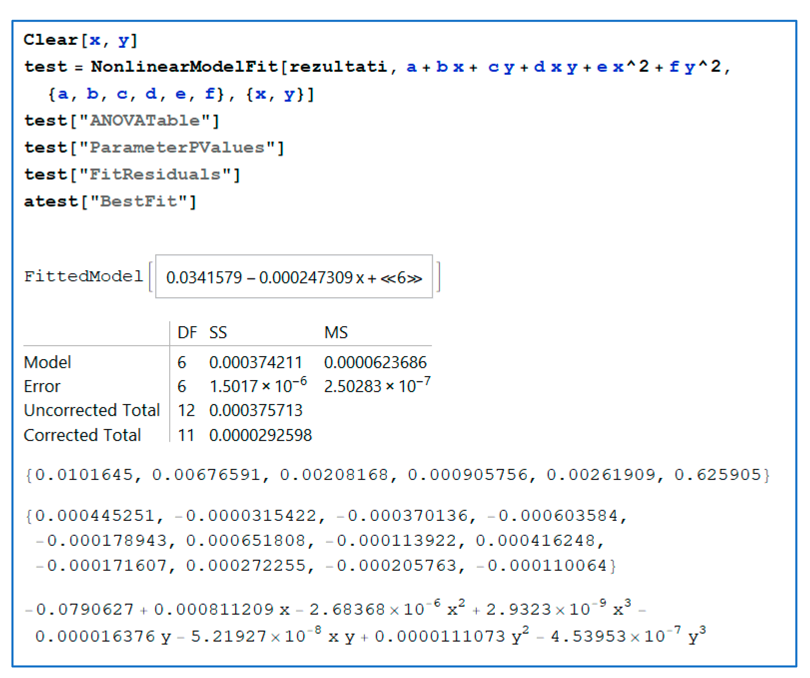
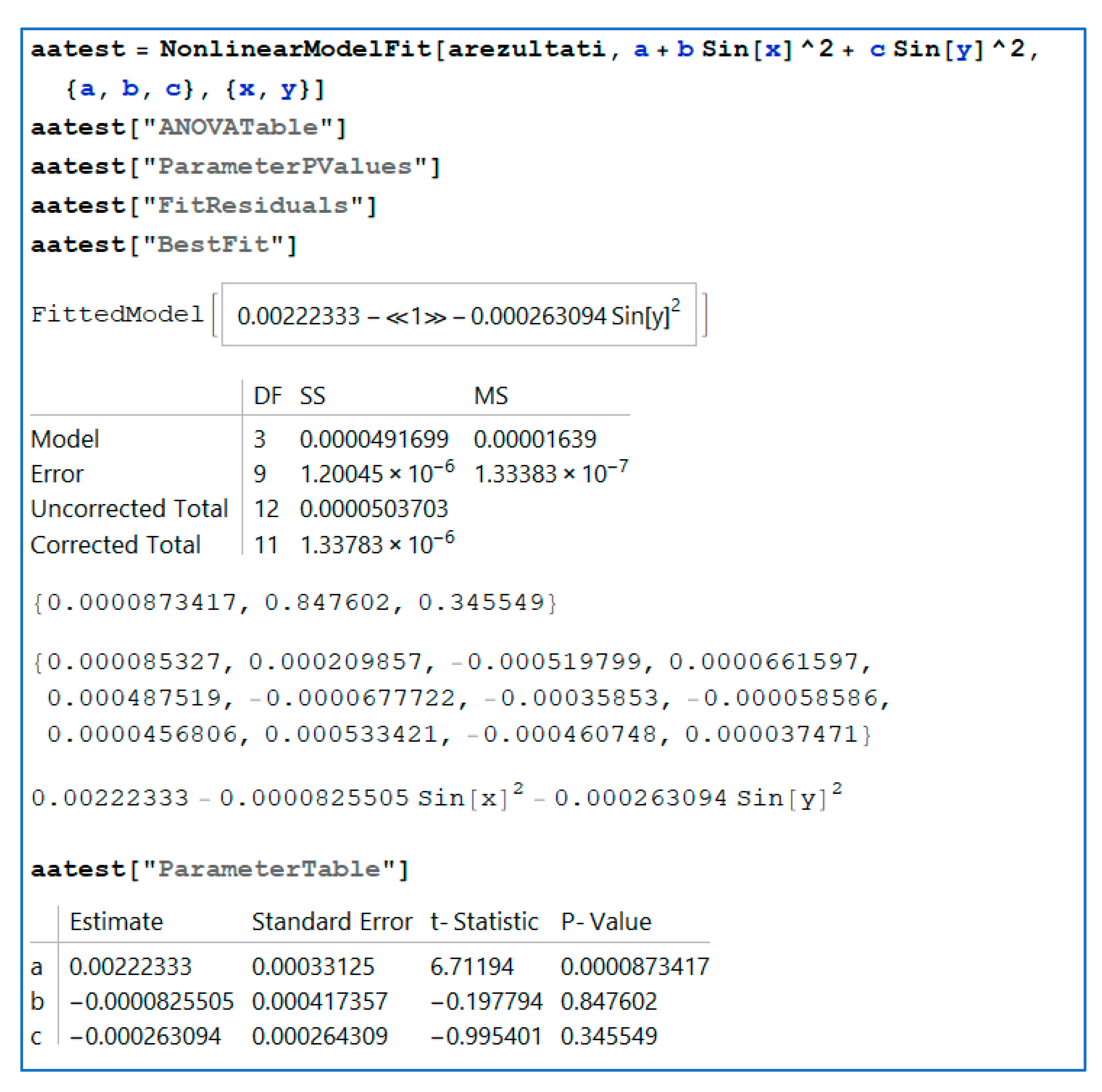
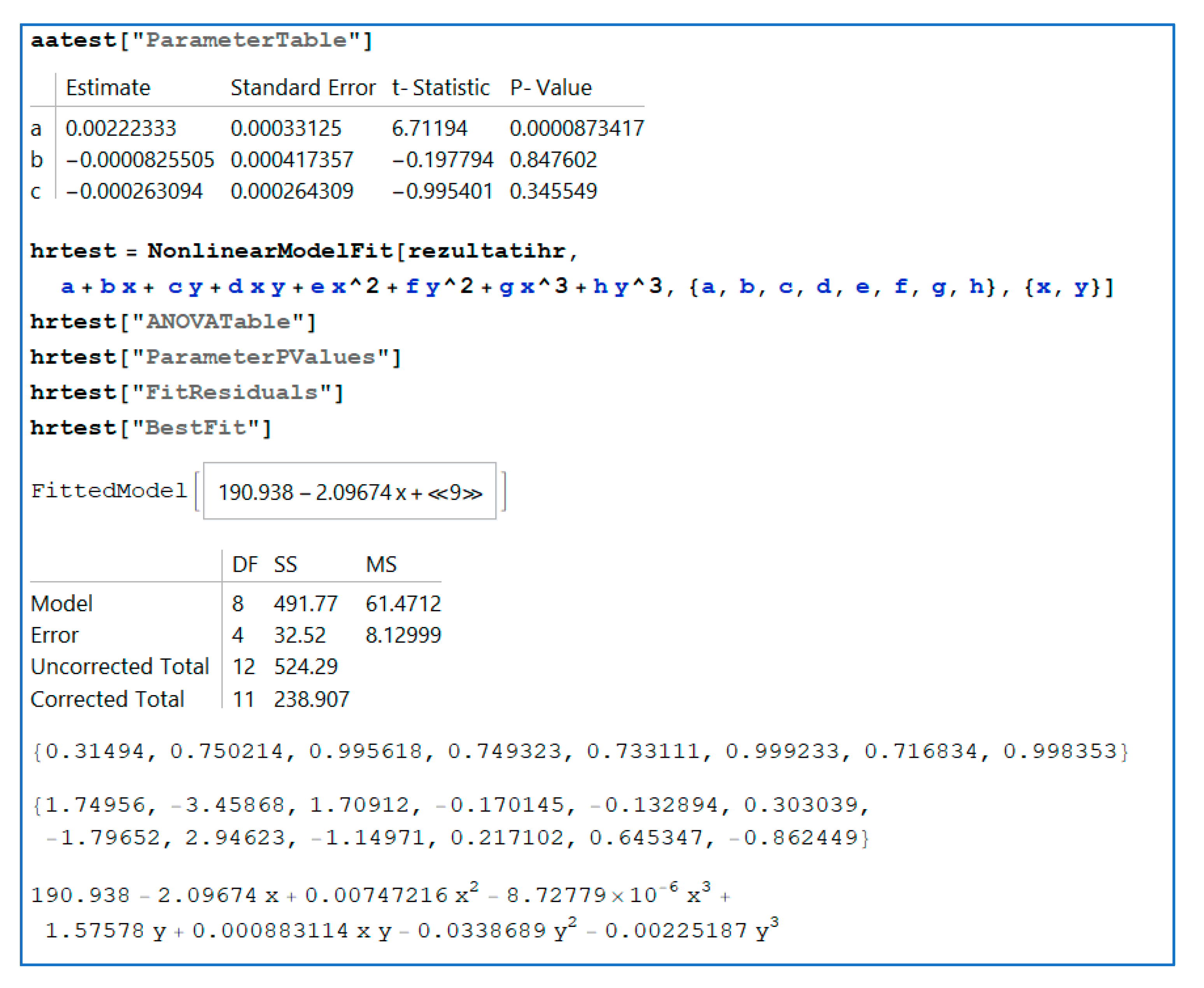
Figure 10, Figure 11 and Figure 12 show the code for the analysis of variance (ANOVA) test for each data set or matrix. Matrix rezultati stores the analyzed vibration data from sensor 1, matrix arezultati stores the analyzed data from vibration sensor 2, and matrix rezultatihr stores data from the surface roughness analysis. With the appropriate function (NonlinearModelFit), ANOVA was performed; the ANOVA table, parameter p values, and residuals were extracted for each prepared set of data.
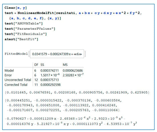
Figure 10.
Results from an analysis of variance (ANOVA) test on RMS data from the first vibration sensor.
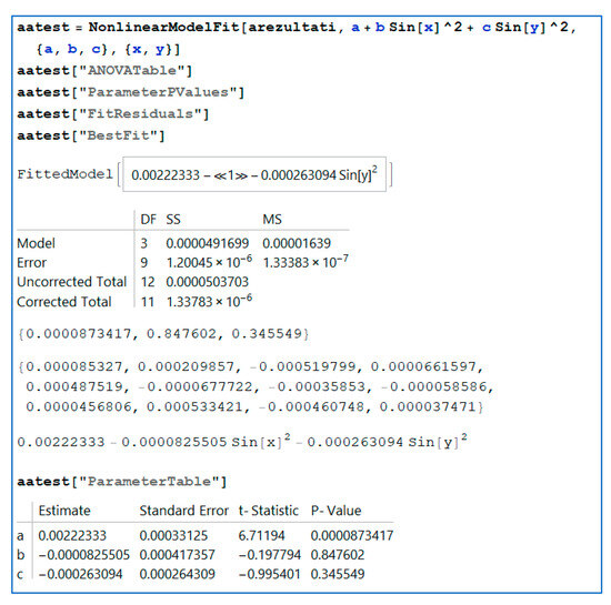
Figure 11.
Results from the ANOVA test on RMS data from the second vibration sensor.
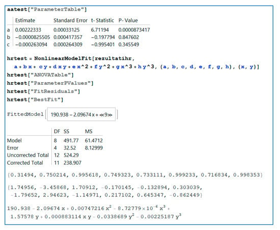
Figure 12.
Results from the ANOVA test on roughness data after the first model proposition.
Figure 11 and Figure 12 show fitted models and the ANOVA results. The ANOVA tests revealed good statistical significance in the first and second sets of vibration data, whereas models of surface roughness indicated that the model was insignificant. However, for this experiment, we proceeded with obtaining the fit function. Further measurements are planned to improve model significance. In particular, the surface roughness will be measured for more levels of input parameters to determine whether the increased number of input parameters would influence the resulting model and increase the level of significance; otherwise, it would prove that the machining parameters do not impact the surface roughness of the workpiece. Additional data transformation may also improve model significance; this will be explored in future research efforts.
Using the data-fitting function of Wolfram Mathematica 10.2 on the data obtained from each acceleration amplitude sensor, the following mathematical models were obtained.
z1(x,y) = 0.03415785900453084 − 0.0002473091590497814x + 4.942675518276936 × 10−7x2
+ 0.0008515342411291489y − 0.000002748337562519144xy
− 0.000001962503643581894y2
z2(x,y) = 0.00222333 − 0.0000825505 Sin[x]^2 − 0.000263094 Sin[y]^2
+ 0.0008515342411291489y − 0.000002748337562519144xy
− 0.000001962503643581894y2
z2(x,y) = 0.00222333 − 0.0000825505 Sin[x]^2 − 0.000263094 Sin[y]^2
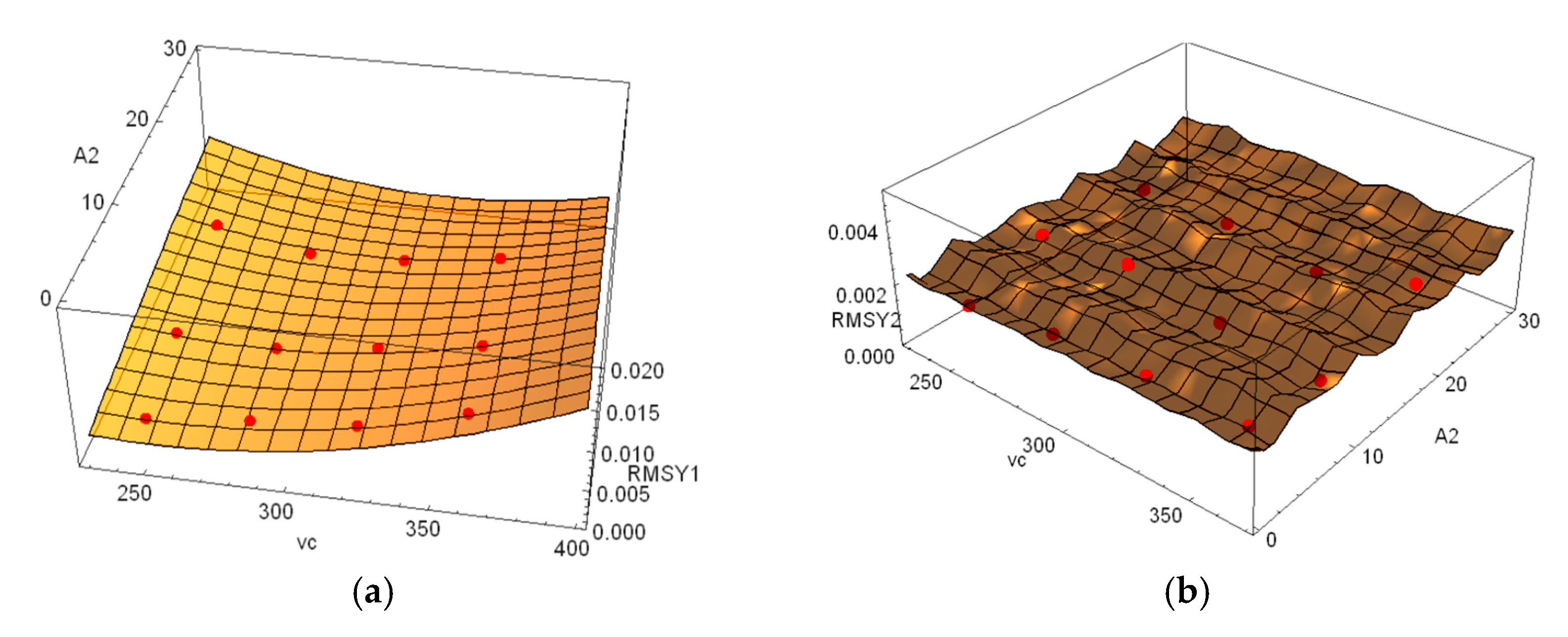
The response surfaces, and measurement points used to derive vibration measurement data for each sensor are shown in Figure 13. The obtained surfaces and three-dimensional graphs show how the machining parameters impact vibration amplitude levels.

Figure 13.
Response surfaces and measurement points used to derive vibration data. (a) Response surface—data sensor 1, (b) Response surface—data sensor 2.
In a similar manner, the Ra value for surface roughness was determined; the response surface is shown in Figure 14. For simplicity, physical units on the following graphs are omitted and can be identified using Table 6.
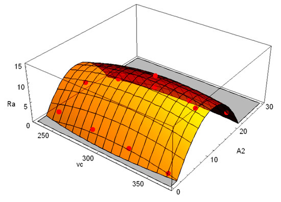
Figure 14.
Response surfaces and measurement points used to derive surface roughness data.
The current model z2 has a form that significantly differs from the response surface of sensor 1. Further measurements are planned to obtain more accurate results for the real model.
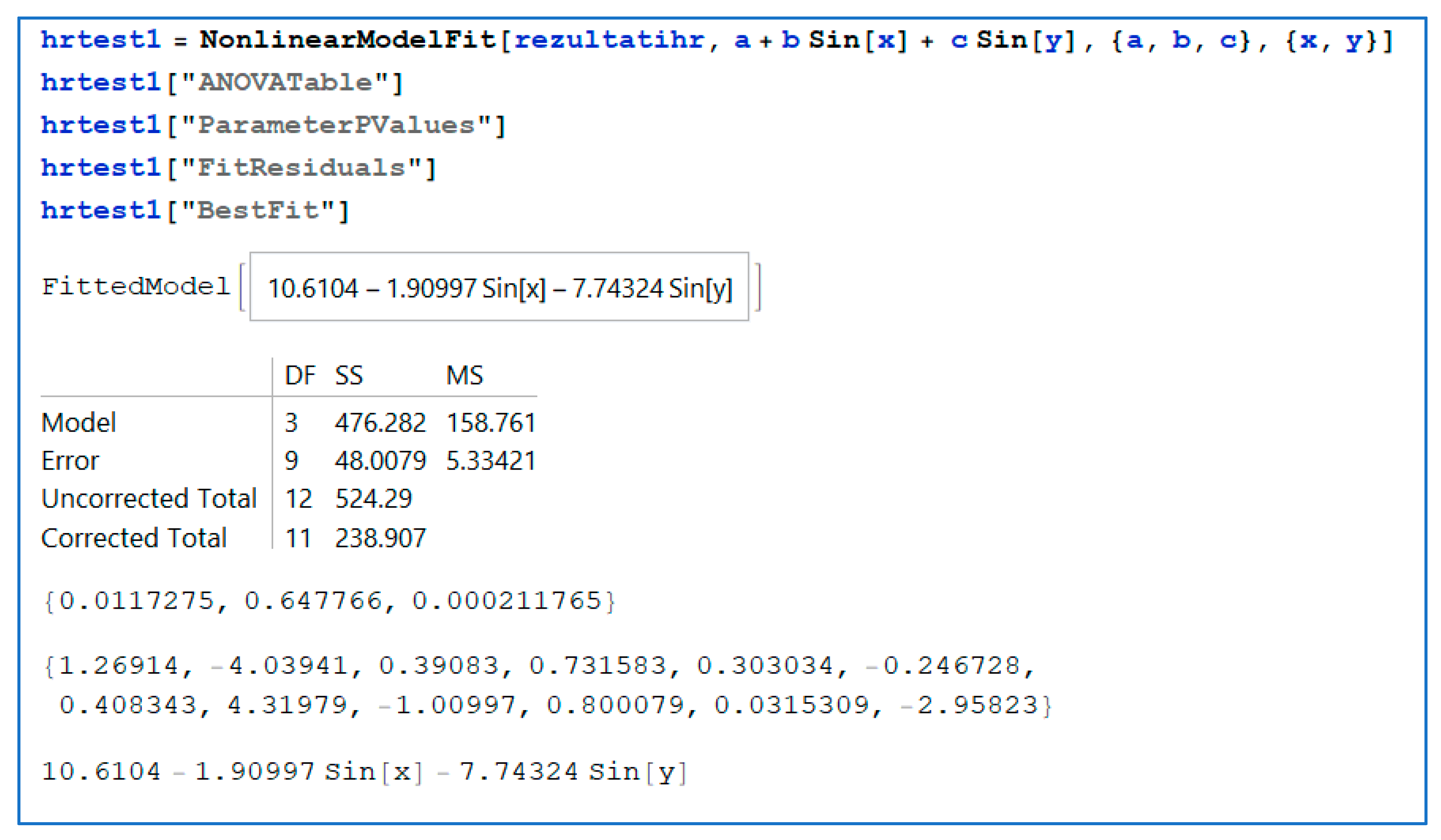
The Wolfram Mathematica 10.2 function was also used to establish the response surface model from roughness measurement data. The impact of machining parameters on surface roughness is shown in Figure 14. Although upon modification of the prediction model, the ANOVA showed an improvement in model significance (Figure 15), the sinusoidal model may not provide the best representation of the data. Additional tests with more input variable levels might improve model significance or help to entirely dismiss the chosen model.
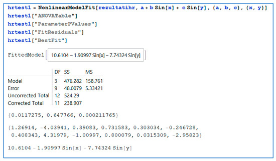
Figure 15.
ANOVA of the reformulated surface roughness model.
The model obtained using the surface roughness data is as follows:
Z3(x,y) = 190.938 − 2.09674 x + 0.00747216 x2 − 8.72779 × 10−6 x3 +
1.57578 y + 0.000883114 xy − 0.0338689 y2 − 0.00225187 y3
1.57578 y + 0.000883114 xy − 0.0338689 y2 − 0.00225187 y3
The response surfaces of the vibration data and surface roughness data were compared. Based on the chosen models, it is apparent that the lowest roughness and vibration values of the surface cross-sections are those that occur at higher cutting speeds and larger A2 values.
5. Conclusions
Screws were produced for a small dry extruder used for soybean processing, employing a universal lathe with a whirling attachment featuring a specially designed cutting head. In total, 14 screws were made, 12 in two passes. Vibrations of the whirling attachment and lathe apron influenced the vibrations and surface qualities of the processed screws; these were measured at four points. Compared to previous studies, a more easily machinable material is now used, and the cutting tool is more precisely positioned. The clearance between the workpiece and the mandrel was reduced to a maximum of 30 μm.
When the cutting speed was lowest, and the cutting depth was highest during the second pass, the measured surface roughness data showed that the quality of the machined surface was optimal. In general, the machined surface quality was enhanced at the highest cutting speed and the lowest cutting depth; the vibrations were minimal. A higher cutting speed also reduced the overall amplitude and vibration energy but was limited by the required tool durability.
The differences in the qualities of the machined surfaces were large, but the arithmetic means ranged from N8 to N9. The surface roughness values differed between the left- and right-screw flanks, but the surface quality was lower after machining commenced because the tool then cut material distant from the lathe chuck, and tool entry into the material caused vibration.
The surface quality of screws machined in two passes was approximately 13% better than that of screws produced previously, but screws produced in one pass exhibited a 34% improvement in surface quality.
The results showed that two-pass machining was not profitable. The final surface quality was poor, tool durability was low, and the production time was long. It is essential to use a highly machinable material and to machine at a cutting speed that is optimized in terms of the major diameter and thread height of the screw.
The overall scientific contribution of this article is the measurement of output data for known input parameters and the determination of the optimal machining parameters. Currently, small production companies in Croatia use conventional machines. Designing special tools and making adjustments to conventional tools can prolong machine life without reducing product quality. This experiment can help product planners choose machining parameters to achieve better workpiece accuracy and improved surface quality.
Author Contributions
Conceptualization, Z.B. and K.P.; methodology, Z.B. and M.H.; software, K.P. and T.T.; validation, Z.B., K.P., M.H. and T.T.; formal analysis, K.P. and T.T.; investigation, Z.B. and K.P.; resources, Z.B., K.P., M.H. and T.T.; data curation, Z.B. and K.P.; writing—original draft preparation, Z.B. and K.P.; writing—review and editing, Z.B., K.P., M.H. and T.T.; visualization, Z.B. and K.P.; supervision, Z.B. and K.P.; funding acquisition, Z.B., K.P., M.H. and T.T. All authors have read and agreed to the published version of the manuscript.
Funding
This research received no external funding.
Data Availability Statement
The data presented in this study are available on request from the corresponding author.
Conflicts of Interest
The authors declare no conflicts of interest.
References
- Creţu, G.; Coteaţă, M. Contributions on the Influence of the Cutting Parameters and Constructive Geometrical Parameters of the Tool on the Precision of the Worm Gears Manufactured Using Whirling Thread Cutting. Appl. Mech. Mater. 2013, 371, 54–58. [Google Scholar] [CrossRef]
- Creţu, G. Contributions on Design and Accomplishing of the Whirling Thread Cutting Devices that could be Adapted for Ordinary Lathes. Adv. Mat. Res. 2013, 837, 67–70. [Google Scholar] [CrossRef]
- Creţu, G. Researches in Cutting Parameters Influence on the Surface Quality in Worms Manufacturing with Whirling Thread Cutting. Adv. Mat. Res. 2014, 1036, 394–398. [Google Scholar] [CrossRef]
- Cretu, G. Contributions to systemic analysis for worm screw production using thread whirling devices. IOP Conf. Ser. Mater. Sci. Eng. 2017, 227, 012032. [Google Scholar] [CrossRef]
- Merticaru, V.; Mihalache, A.; Nagîţ, G.; Dodun, O.; Slătineanu, L. Some Aspects about the Significant Parameters of the Thread Whirling Process. Appl. Mech. Mater. 2016, 834, 96–101. [Google Scholar] [CrossRef]
- Song, S.; Zuo, D. Modelling and simulation of whirling process based on equivalent cutting volume. Simul. Model Pr. Theory 2014, 42, 98–106. [Google Scholar] [CrossRef]
- Soshi, M.; Rigolone, F.; Sheffield, J.; Yamazaki, K. Development of a directly-driven thread whirling unit with advanced tool materials for mass-production of implantable medical parts. CIRP Ann. 2018, 67, 117–120. [Google Scholar] [CrossRef]
- Wang, L.; He, Y.; Li, Y.; Wang, Y.; Liu, C.; Liu, X.; Wang, Y. Modeling and analysis of specific cutting energy of whirling milling process based on cutting parameters. Procedia CIRP 2019, 80, 56–61. [Google Scholar] [CrossRef]
- Han, L.; Liu, R.; Liu, X.; Feng, J. Theoretical modeling and chatter prediction for the whirling process of airfoil blades with consideration of asymmetric FRF and material removal. Int. J. Adv. Manuf. Technol. 2020, 106, 2613–2628. [Google Scholar] [CrossRef]
- Botak, Z.; Pisačić, K.; Horvat, M.; Ficko, M. Manufacture of soybean extruder screws using a lathe with a whirling attachment. Int. J. Mach. Mach. Mater. 2022, 24, 350. [Google Scholar] [CrossRef]
- Igba, J.; Alemzadeh, K.; Durugbo, C.; Eiriksson, E.T. Analysing RMS and peak values of vibration signals for condition monitoring of wind turbine gearboxes. Renew Energy 2016, 91, 90–106. [Google Scholar] [CrossRef]
- Khan, D.; Burdzik, R. Measurement and analysis of transport noise and vibration: A review of techniques, case studies, and future directions. Measurement 2023, 220, 113354. [Google Scholar] [CrossRef]
- Twardowski, P.; Czyżycki, J.; Felusiak-Czyryca, A.; Tabaszewski, M.; Wiciak-Pikuła, M. Monitoring and forecasting of tool wear based on measurements of vibration accelerations during cast iron milling. J. Manuf. Process. 2023, 95, 342–350. [Google Scholar] [CrossRef]
- Malmborg, J.; Flodén, O.; Persson, P.; Persson, K. Numerical study on train-induced vibrations: A comparison of timber and concrete buildings. Structures 2024, 62, 106215. [Google Scholar] [CrossRef]
- Norén-Cosgriff, K.; Ellingsen, S.; Resvoll, R.; Hov, S. The new museum of the Viking Age—Assessment of vibration from groundworks to avoid damage to artefacts. Appl. Acoust. 2022, 196, 108862. [Google Scholar] [CrossRef]
- Pisačić, K.; Botak, Z.; Horvat, M. An Overview and Efficiency Analysis of Dominant Frequencies Estimation Methods with the Application of DIRECT Global Minimization Method. Teh. Vjesn.—Tech. Gaz. 2020, 27, 1685–1693. [Google Scholar] [CrossRef]
- Wolfram Research. Fit, Wolfram Language Function. 1988. Available online: https://reference.wolfram.com/language/ref/Fit.html (accessed on 8 May 2024).
Disclaimer/Publisher’s Note: The statements, opinions and data contained in all publications are solely those of the individual author(s) and contributor(s) and not of MDPI and/or the editor(s). MDPI and/or the editor(s) disclaim responsibility for any injury to people or property resulting from any ideas, methods, instructions or products referred to in the content. |
© 2024 by the authors. Licensee MDPI, Basel, Switzerland. This article is an open access article distributed under the terms and conditions of the Creative Commons Attribution (CC BY) license (https://creativecommons.org/licenses/by/4.0/).

