Abstract
Since tool wear accumulates in the cutting process, the condition of the cutting tool shows a degradation trend, which ultimately affects the surface quality. Tool wear monitoring and prediction are of significant importance in intelligent manufacturing. The cutting signal shows short-term randomness due to non-uniform materials in the workpiece, making it difficult to accurately monitor tool condition by relying on instantaneous signals. To reduce the impact of transient fluctuations, this paper proposes a novel network based on deep learning to monitor and predict tool wear. Firstly, a CNN model based on residual connection was designed to extract deep features from multi-sensor signals. After that, a temporal model based on an encoder and decoder was built for short-term monitoring and long-term prediction. It captured the instantaneous features and long-term trend features by mining the temporal dependence of the signals. In addition, an encoder and decoder-based temporal model is proposed for smoothing correction to improve the estimation accuracy of the temporal model. To validate the performance of the proposed model, the PHM dataset was used for wear monitoring and prediction and compared with other deep learning models. In addition, CFRP milling experiments were conducted to verify the stability and generalization of the model under different machining conditions. The experimental results show that the model outperformed other deep learning models in terms of MAE, MAPE, and RMSE.
1. Introduction
Traditional manufacturing is undergoing a transformation towards intelligent manufacturing with the development of information technology, demanding intelligent and automated upgrades in machining [1]. In the machining process, tool wear is inevitable, which directly affects the tool surface integrity and machining accuracy, and may even damage the machine tool [2,3,4]. Relevant studies have shown that 10–40% of machine tool downtime is caused by abnormal tool conditions [5] and the service life of tools is only 50–80% of the recommended service life [6]. Therefore, tool condition monitoring (TCM) offers advantages in cutting costs and enhancing production efficiency and product quality, and holds significance for smart manufacturing.
Two methods are commonly applied in TCM, namely, direct and indirect methods. For the direct method, the tool wear is directly measured with an optical microscope or a CCD camera based on computer vision methods [7]. In the indirect method, models of TCM are established based on signals collected by sensors, such as cutting force [8], vibration [9], acoustic emission [10], and spindle power [11]. Compared with direct methods that require machine tools to be shut down for measuring, indirect methods allow in situ estimates of tool condition based on sensor data. Consequently, indirect methods are considered to be more suitable for in situ tool condition monitoring.
Many models have been proposed for indirect TCM, including physical models, data-driven models, and hybrid models. Most physical models consider only the dominant factors related to tool wear, which have the advantages of low complexity and physical interpretability, but require expert domain knowledge to construct [12]. Hybrid models combine physical knowledge with data-driven models, easing the lack of sample data and improving its generalization ability [13,14]. However, the applied physical knowledge mainly relies on prior information about tool wear and lacks deep embedding of tool wear mechanisms. In addition, these methods require large-scale tool wear labels for model training, which make it difficult to meet the needs of online prediction. Data-driven models use accurate mapping between features and wear to solve tool condition monitoring problem. Liao et al. [15] proposed a method based on acoustic emission signals using wavelet packet decomposition to extract energy features; a support vector machine (SVM) model was established for TCM. Li et al. [16] proposed a time varying and condition adaptive hidden Markov model for capturing tool wear time dependence. Chen et al. [17] proposed an artificial neural network-based in-process tool wear prediction (ANN-ITWP) model, estimating the tool wear values by cutting parameters and average peak force in the y direction. Cheng et al. [18] used a support vector regression (SVR) model to estimate tool flank wear, with a grid search algorithm (GS), a genetic algorithm (GA), and particle swarm optimization used for parameter optimization. The prediction accuracy of the proposed method was 97.32% and 96.72% under GA-SVR and GS-SVR prediction models, respectively. The abovementioned machine learning models have achieved considerable success in TCM. However, they require a lot of feature engineering work in feature extraction and screening [19,20].
Deep learning has a strong ability to extract features automatically compared with traditional machine learning methods, with no necessity to perform feature engineering. Therefore, many deep learning models have been proposed for TCM in recent studies. CNN can extract spatial relationship from the feature map through the combination of convolution layers and pooling layers. Xu et al. [21] proposed a multi-scale feature fusion implemented by the developed parallel convolutional neural networks. The channel attention mechanism combined with the residual connection was developed to enhance the performance of the model. Duan et al. [22] enlarged samples and applied a three-layer wavelet package decomposition. A multi-frequency-band feature extraction structure based on a deep convolution neural network structure was introduced to predict tool wear conditions. Yong et al. [23] proposed a one-dimensional convolutional neural network (1D-CNN) and deep generalized canonical correlation analysis (DGCCA). In particular, 1D-CNN was used to extract features from 1D raw data, whereas DGCCA with attention mechanism was used to fuse the feature output from each 1D-CNN. Shah et al. [24] extracted image quality parameters from scalograms constructed from Morlet wavelets, and built several LSTM models for tool wear prediction. Wu et al. [25] applied a feature extraction method based on singular value decomposition (SVD) and used a BiLSTM model to predict tool wear. Zhang et al. [26] used 1D-CNN to automatically extract features, and then used BLSTM model to mine time-dependency of features and monitor tool wear. Xu et al. [27] proposed an integrated model based on deep learning and multi-sensory feature fusion; the proposed parallel convolutional neural network (PCNN) achieved multi-sensory feature fusion. The prediction results were generated by a fully connected neural network.
Existing deep learning models studies mostly focus on tool condition monitoring, with less attention on tool wear prediction. The significance of tool wear prediction lies in achieving early warning of tool condition and reducing the probability of outliers. In this paper, a novel method for tool wear monitoring and prediction is proposed based on a residual convolutional network and seq-to-seq structure. The contributions of this work are as follows:
- (1)
- A deep convolutional network based on a residual structure is proposed to achieve multi-scale feature fusion of multi-source information and alleviate the problems of gradient disappearance and performance degradation. In addition, the introduction of BN and dropout layers improves the generalization ability of the model and avoids overfitting.
- (2)
- An encoder–decoder network for short-term monitoring and long-term prediction was built based on the attention mechanism. It can capture the time dependence of depth features, as well as the instantaneous features and long-term trends of time series features.
- (3)
- The encoder and decoder-based temporal model can be used for in-process smoothing to reduce local fluctuations in wear values, which improves monitoring and prediction accuracy compared to traditional smoothing methods.
The rest of paper is organized as follows. Section 2 introduces the theoretical background of CNN and temporal model. In Section 3, the proposed model for tool condition monitoring and prediction are introduced. Then, the experiment is presented and the results are discussed in Section 4. Finally, conclusions are drawn in Section 5.
2. Theoretical Framework
2.1. Residual Convolutional Network
2.1.1. Convolutional Neural Network
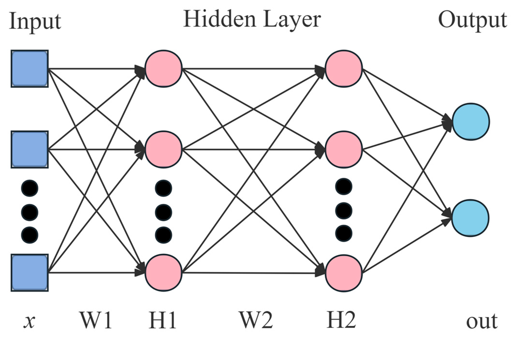
A CNN is a type of feedforward network, which is among the representative models of deep learning [28]. Widely employed in image recognition, video classification and more [29], CNNs show a powerful capability of representation learning, allowing them to perform feature extraction and reduce spatial dimensionality of feature maps through convolution and pooling. As shown in Figure 1, the structure of a CNN includes an input layer, a convolutional layer, a pooling layer, activation function, and a fully connected layer.

Figure 1.
The architecture of a convolutional neural network.
Convolutional layers contain kernels that can extract features from input data, with each kernel having a set of weight and bias that can be learned. Parameters of the model are optimized through learning, aiming to learn feature representation of the inputs. A convolutional layer can be expressed as follows:
where is the (l − 1)th feature map of the input, is the lth feature map, is the kernel of the lth layer, M represents the size of input, is bias of the lth layer, and f represents the activation function.
A pooling layer is used to decrease the dimensions of feature maps and minimize the number of parameters, reducing the required computations and alleviating the issue of overfitting. Pooling methods include maximum pooling and average pooling. The former is used in this paper, which can be expressed as follows:
where is the input feature map of the lth layer and S represents the pooling window size.
After convolutional and pooling layers, fully connected layers are adopted to apply a linear transformation to the input vector, and a nonlinear transformation is then performed through an activation function to obtain the output. The output layer can be expressed as follows:
where w is the weight between the lth and l – 1th layer, x is the output value of the ith neuron in the l – 1th layer, b is the bias of the jth neuron in the lth layer, and represents the activation function.
2.1.2. Residual Structure
A residual neural network (ResNet) is a deep learning model proposed by He et al. [30] to alleviate the gradient vanishing and network degradation when the layers increase. A ResNet applies residual joins to map features to layer inputs and merges them with outputs by addition, as shown in Figure 2.
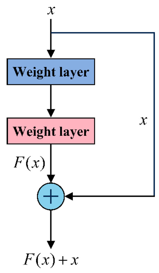
Figure 2.
The architecture of a residual network block.
The input is x, and the residual is defined as F(x), which is the difference between features Y(x) learned from convolution layers and input. The residual F(x) is learned during training with expectation of convergence to 0, resulting in an identity mapping Y(x) = x. Residual connection not only retains the advantages of a shallow network, but also alleviates network degradation and enables building of deeper networks. The residual connection can be represented as follows:
2.2. Temporal Model
2.2.1. Gated Recurrent Unit
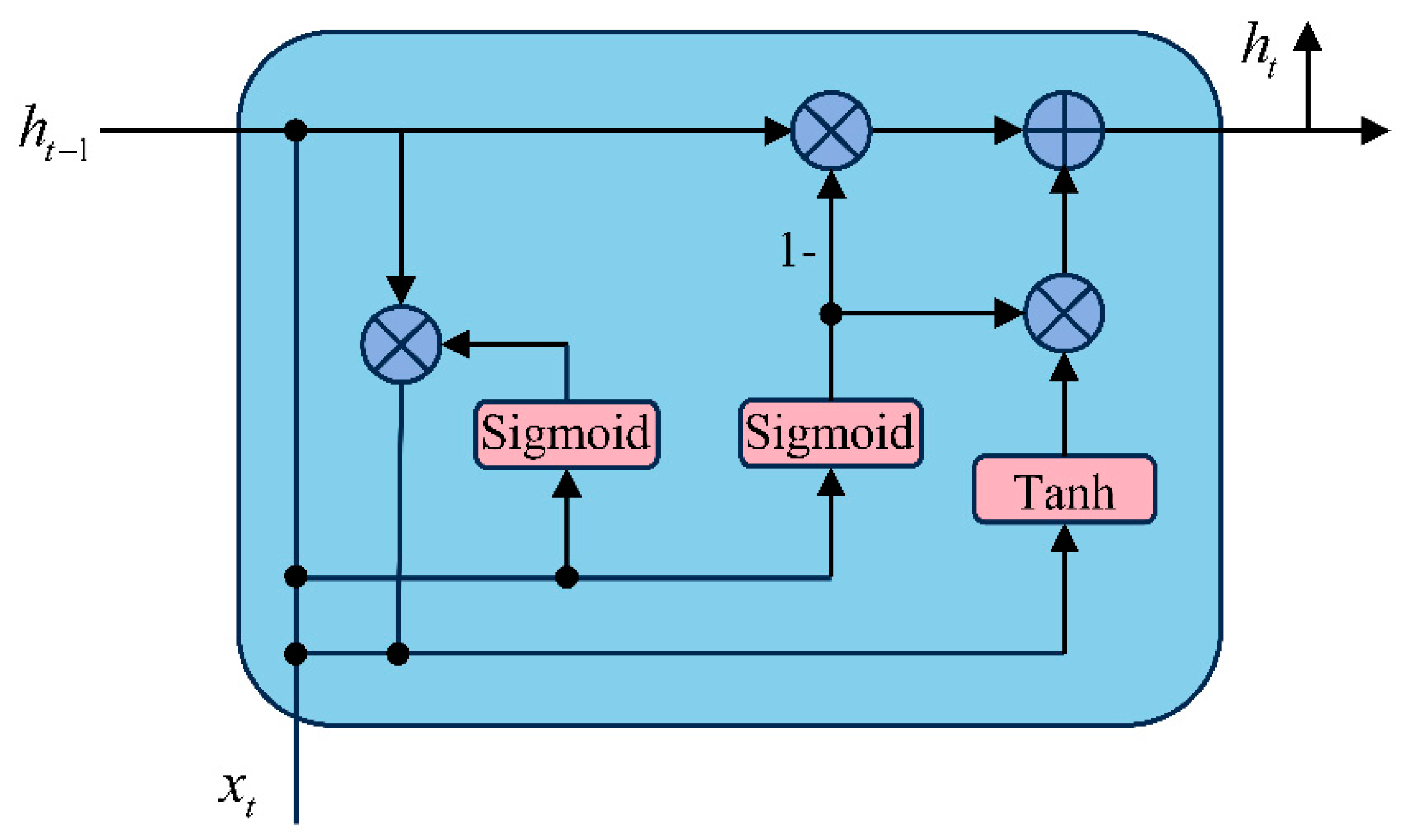
A gate recurrent unit (GRU) is an improved version of a recurrent neural network (RNN) [31], with a gating mechanism introduced to modulate the flow of information, as shown in Figure 3. Compared with the original RNN, the superiority of a GRU lies in two gate control units: a reset gate and an update gate. Its expression is as follows:
where is the input of the t-th moment, is the hidden state of the t – 1th moment. The update gate determines how much historical information needs to be retained for the current state, controlling information that flows into memory. The reset gate decides how much of the previous state to forget, controlling the information that flows out of memory. With the gating mechanism, a GRU handles long-term time-dependency more effectively than the original RNN, which alleviates the problem of vanishing gradient.
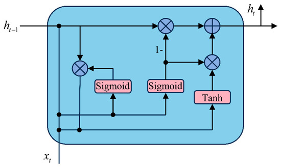
Figure 3.
The architecture of a GRU unit.
2.2.2. Encoder–Decoder
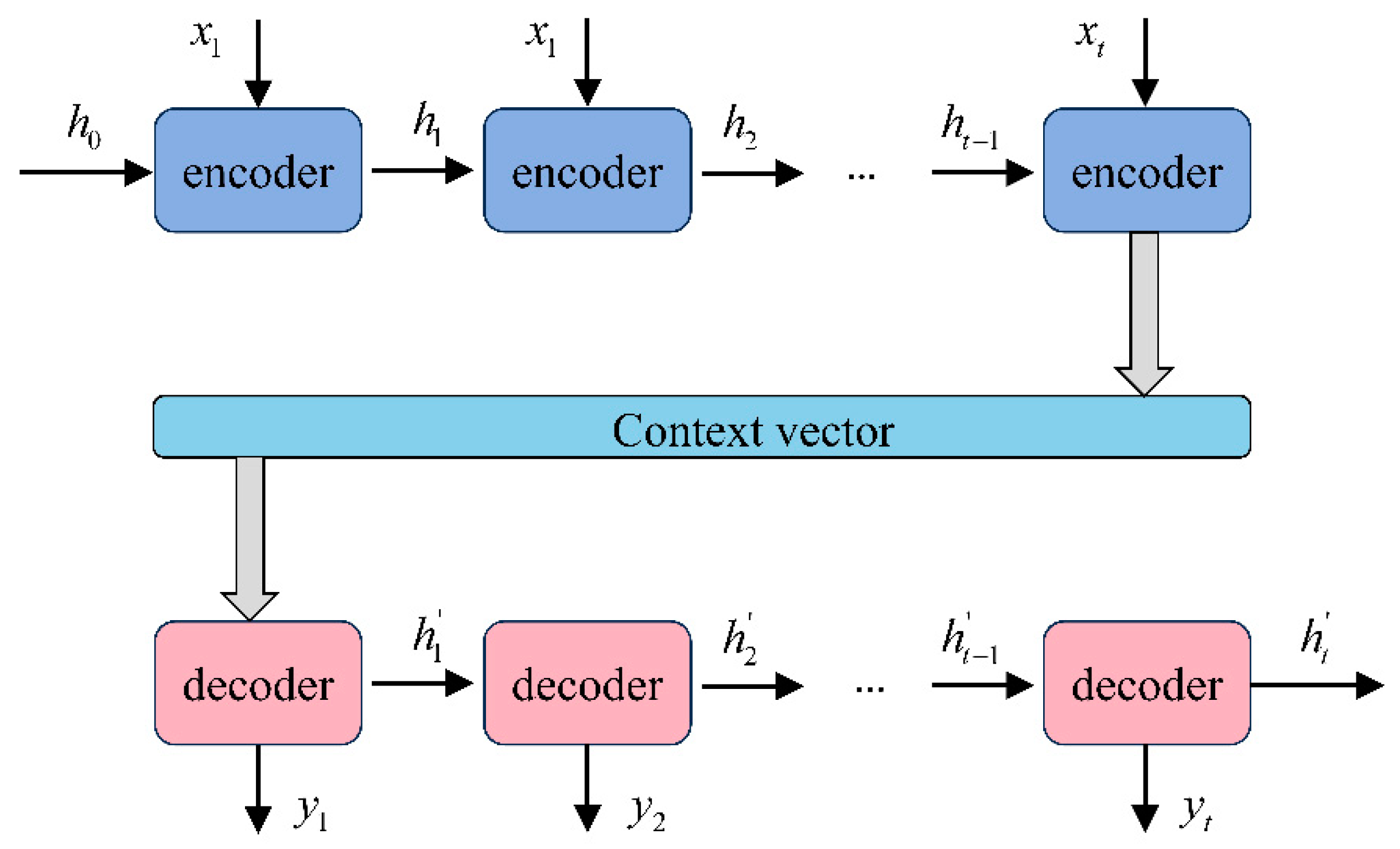
A sequence-to-sequence model is a deep learning technique widely applied in machine translation and speech recognition [32]. It is an encoder- and decoder-based model that maps an input sequence to an output sequence. The model consists of two main components: an encoder and a decoder, as shown in Figure 4. The encoder and decoder are typically implemented by a RNN or improved versions such as LSTM and GRU.
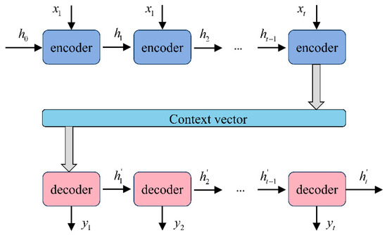
Figure 4.
The structure of an encoder and a decoder.
The encoder is used to summarize information from input sequences and convert inputs to vectors of fixed length. The inputs of the encoder can be vectors or a sequence of words with variable length. A hidden state vector is generated by the encoder, which represents the context of the input sequence. The final hidden state of the encoder, namely the semantic vector, is then passed to the decoder as an input.
The decoder, used in conjunction with the encoder, works similarly to the encoder. It takes the semantic vector generated by the encoder and current hidden states as inputs. At each time step, the input vectors are fed into decoder and the next hidden state is output until the end of the output sequence.
2.2.3. Encoder–Decoder with Attention
An attention mechanism is an artificial intelligence technique that enables networks to focus on a subset of features by learning the weight and improving the performance of networks in processing sequence data [33].
There exist limitations, though encoders and decoders have been widely used for sequence processing tasks. Encoders and decoders are associated with a semantic vector, which is expected to represent the information of the entire sequence. Since they have a limited memory capacity and inability to preserve early historical information, semantic vectors cannot reflect the whole sequence, reducing the accuracy of decoder outputs.
To address these issues, the encoder and decoder modules introduce an attention mechanism. At each moment, the attention layer generates a semantic vector based on the information of the input sequence. Each intermediate vector contains different degrees of long-term and short-term information, the degree of which depend on the amount of weight given by the attention mechanism. The decoder generates an output vector based on the semantic vector. The attention mechanism is less dependent on the whole sequence, which improves the generalization ability and interpretability of the network. The attention mechanism of the encoder–decoder model can be expressed as follows:
where is the ith hidden layer of the encoder, and is the (j − 1)th hidden layer of the decoder. is Euclidean distance between and . is the weight of the ith hidden layer of the encoder, and is the semantic vector.
3. Methodology
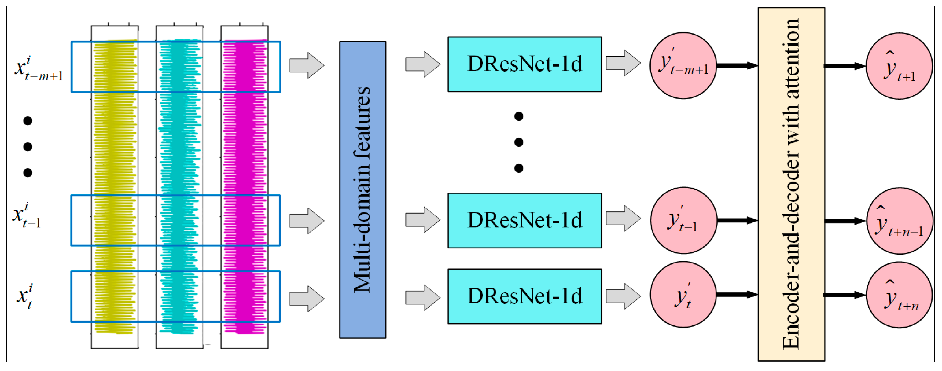
In this paper, a hybrid model based on 1D-CNN and Resnet (DResnet-1d) is proposed for tool condition monitoring, on the basis of which tool condition prediction is carried out by a time-series model to achieve early warning of tool condition, as shown in Figure 5. The sensor signals collected during machining and the corresponding tool wear values are put into the proposed model. Model training determines the optimal parameters of the proposed model. The initial estimates are transferred to a multi-step predictive time-series model. Through smoothing corrections, tool wear monitoring and prediction can be achieved.
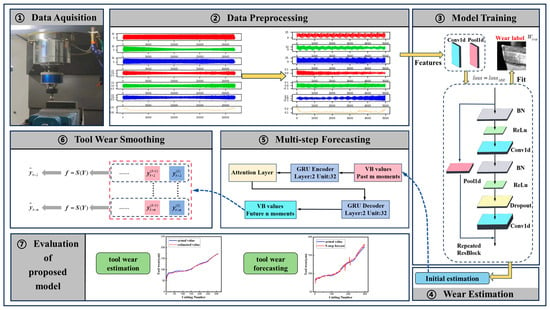
Figure 5.
The tool condition monitoring and predicting system.
3.1. Deep Feature Extraction for Tool Wear
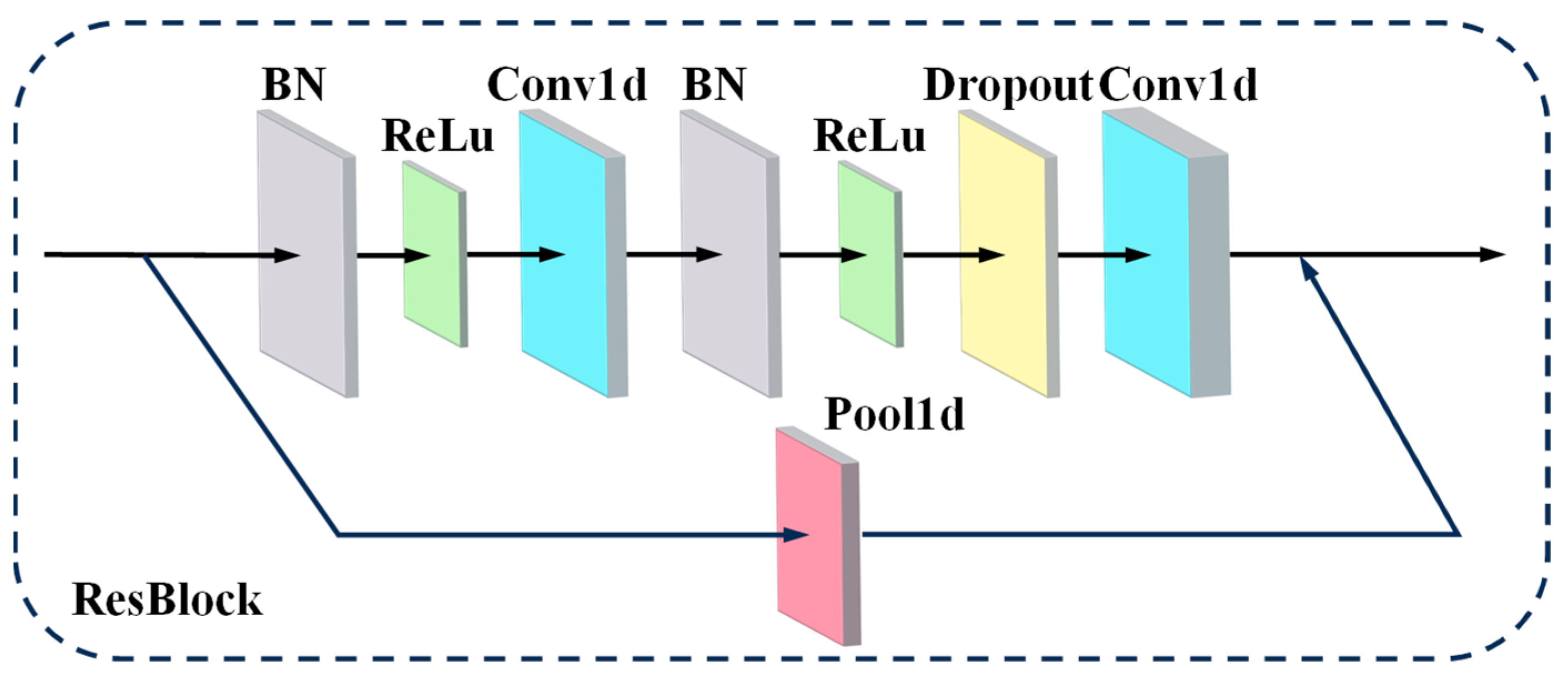
A deep network is supposed to have an excellent capability of feature extraction by assembling elementary features in shallow layers into advanced features in deep layers. For this paper, a DResNet-1d model was established to estimate tool wear values, as shown in Figure 6. The convolutional unit at the beginning was used to fuse multi-sensor data and transform the number of channels of the feature map. ResBlock represents a residual block, the structure of which refers to the pre-activation residual block [34] shown in Figure 7. Conv is the convolution layer, BN represents the BatchNorm layer, dropout represents the dropout layer, and the activation function is ReLU. The number of convolution kernels in the residual block is 64 and 128, with strides of 1 and 2, and the kernel size is 3. In this paper, the ResBlock was set to repeat 20 times to form a deep network. FC is the full connection layer, which is used to nonlinearly map the features into tool wear values.

Figure 6.
DResNet-1d model.

Figure 7.
The structure of ResBlock.
The inputs and outputs of the model can be represented as Equation (7). The input of the model is , where n is the number of sensor signal channels, to is the signal collected by sensor, D represents the model, and the output is the tool wear estimation.
3.2. Multi-Step Prediction Model for Tool Wear
Tool wear is a continuous process, and there exists a temporal correlation between adjacent tool wear values. Considering the ability of a RNN to capture time dependency, an encoder- and decoder-based temporal model was established to achieve long-term and short-term predictions with historical information.
The encoder- and decoder-based temporal model, which is shown in Figure 8a, adopts a GRU based encoder–decoder structure and applies the attention mechanism. The inputs of the encoder are the tool wear values of past moments, and the semantic vector is output by the encoder. The attention layer assigns a weight to the semantic vector at each respective moment, which is fed into the decoder as the initial hidden state, and then tool wear prediction of future moments is output, as shown in Figure 8b.
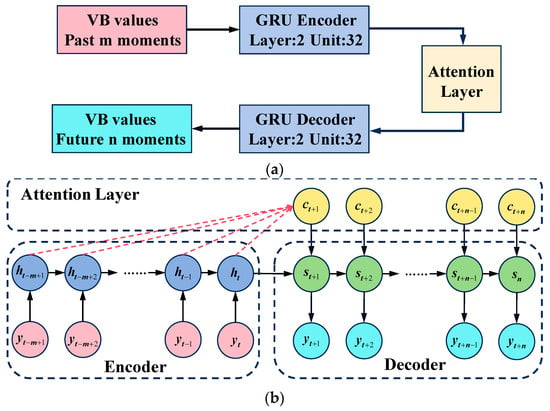
Figure 8.
Multi-step prediction model. (a) The structure of an encoder- and decoder-based temporal model. (b) Inputs and outputs of the temporal model.
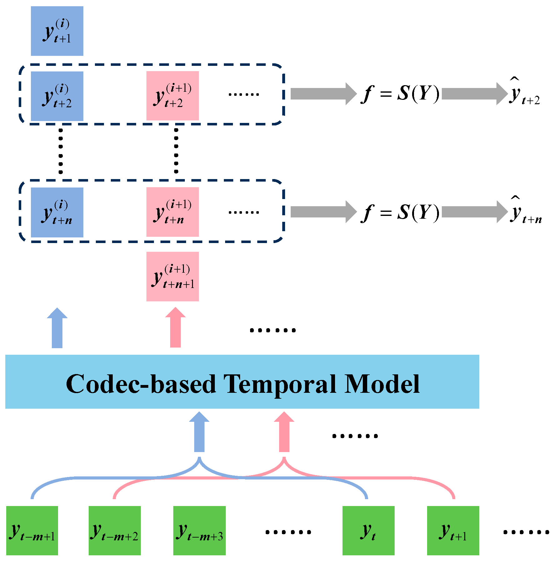
The integrated model for multi-step prediction of tool wear is used to construct an intrinsic link between multi-domain features of multi-channel signals and multi-step wear values. The continuous historical wear values obtained in the monitoring model are used as inputs to the time-series model and the information in the historical wear values is extracted by attention for the prediction of short-term and long-term wear values. The whole process can be expressed as Equation (8). The monitoring model reads the multichannel features to obtain the historical wear values , G represents the monitoring model, and the temporal model takes the tool wear values of past m consecutive moments as inputs of the encoder, denoted as , and F represents the temporal model. The outputs of the decoder are the tool wear predictions of the next n moments, denoted as . The process is shown as Figure 9.
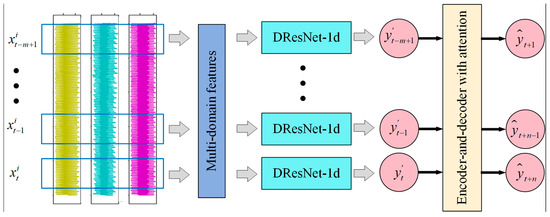
Figure 9.
Comprehensive multi-step model for tool wear prediction.
3.3. Smoothing of Estimation
The DResNet-1d model achieves multi-sensor signal fusion that reduces the impact of signal fluctuations on tool wear estimation. However, there is a lack of temporal correlation between the estimation of adjacent moments, which results in inevitable outliers. To address these shortcomings and inspired by the temporal model, smoothing correction was applied in this paper to reduce the probability of outliers and improve the accuracy of the estimation, as shown in Figure 10.
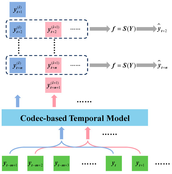
Figure 10.
The smoothing process.
The smoothing correction model adopted in this section follows the aforementioned encoder- and decoder-based temporal model. The historical tool wear values are fed into the model and a short-term prediction is output. Multiple predicted tool wear values exist at each moment, which can be denoted as . The statistical characteristic of available predicted tool wear values at each moment is selected to perform smoothing correction. The smoothing correction can be expressed as follows:
where S represents the function used to calculate statistical features.
4. Experiment
4.1. Description of Dataset
The PHM2010 dataset was used for model verification. The milling experiment was conducted on the Roders Tech RFM760 high-speed CNC milling machine (Roders, Soltau, German). A 6 mm three-flute carbide milling cutter was used in the experiment, and the workpiece material was stainless steel (HRC52, USA). The cutting speed of the workpiece was 196 m/min, and the feed speed in the X-axis direction was set to 1550 mm/min. The cutting depth in the Y-axis direction and Z-axis direction were respectively set to 0.125 mm and 0.2 mm. The tool cut from the upper edge to the lower edge of the workpiece surface in a serrated manner. During the milling process, the cutting length of each tool was about 0.1125 m × 315 = 35.44 m. To obtain tool wear data, the experiment platform was equipped with three types of sensors to measure cutting force, vibration, and acoustic emission signals during machining process. A Kistler three-component dynamometer was installed between workpiece and milling machine to measure the cutting force signals in the X, Y, and Z directions. Further, three Kistler acceleration sensors were installed on the workpiece to measure vibration signals in the three directions, and a Kistler acoustic emission sensor was used to measure the ultra-high frequency stress wave pulse signal released during material deformation. The data obtained from the sensors were processed by a Kistler 5019A multichannel charge amplifier. All measured signals were collected using a data acquisition card (NI DAQ PCI 1200, Texas, USA) at a frequency of 50 kHz. The experiment platform is displayed in Figure 11a. Finally, a total of seven channels of signals were collected, namely the X-direction force (N), Y-direction force (N), Z-direction force (N), X-direction vibration (g), Y-direction vibration, (g), Z-direction vibration (g), and acoustic emission signal (V). In addition, the actual wear of the milling cutter was measured using a LEICA MZ12 microscope (German) after each cutting.
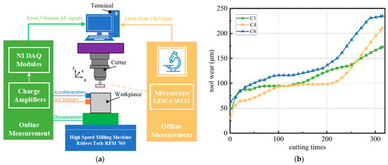
Figure 11.
PHM2010 dataset. (a) Experimental platform and (b) tool wear of C1, C4, and C6.
A total of six datasets corresponding to the wear data of six identical tools were collected under the same conditions as in the milling experiment, recorded as C1, C2, C3, C4, C5, C6, and the number of the cutting time in each dataset was 315. In these datasets, only C1, C4, and C6 measured actual tool wear values after each cutting, as shown in Figure 11b. This paper focuses on a supervised learning model. The C1, C4, and C6 data were used for validation experiments.
4.2. Data Preprocessing
As the cutting number increases, tool wear will intensify, which results in increases in the cutting force and changes in the amplitude of vibration. In addition, acoustic emission signals can reflect the elastic energy of workpiece deformation during processing [35]. Consequently, all seven channels of signals were selected from the PHM2010 dataset for model verification in this paper. Due to the complexity of the machining process and the interference of the experiment environment, the collected signals were inevitably mixed with invalid values, outliers, and noise, which reduced the signal quality. Therefore, the original signals could not be directly fed into the model. To improve the effectiveness of the signal, data preprocessing was applied to the signals before model verification.
The start and end of each cutting process corresponded to the process of tool feeding and retracting. During the tool feeding and retracting, the milling cutter did not come into normal contact with the workpiece, so the signals measured by the sensors may have experienced temporarily invalid data. To eliminate this invalid data, 5% of the data at the start and end part of signals was removed in this paper. This method is simple and had little impact on the data, but effectively removed invalid values from the data.
Three acceleration sensors were used to collect vibration signals in X, Y, and Z directions since the vibration signals came directly from the cutting area with high sensitivity and a short response time. However, due to the interference in the experiment environment and the accuracy of the sensors, there inevitably existed a large amount of noise. Therefore, it was necessary to perform denoising on the collected vibration signals. In signal preprocessing, noise is usually considered Gaussian noise. In this paper, a wavelet threshold denoising method was used for signal denoising [36].
The sampling frequency of the original signal was 50 kHz, resulting in the length of the signal generated in each cutting being up to about 200,000. Additionally, the data collected in each cut were not of uniform length. In order to reduce computational complexity and storage space usage, this paper adopted the segmented aggregation approximation (PAA) method to compress the time series data to a length of 5000. This reduced the data volume, and unified the data length.
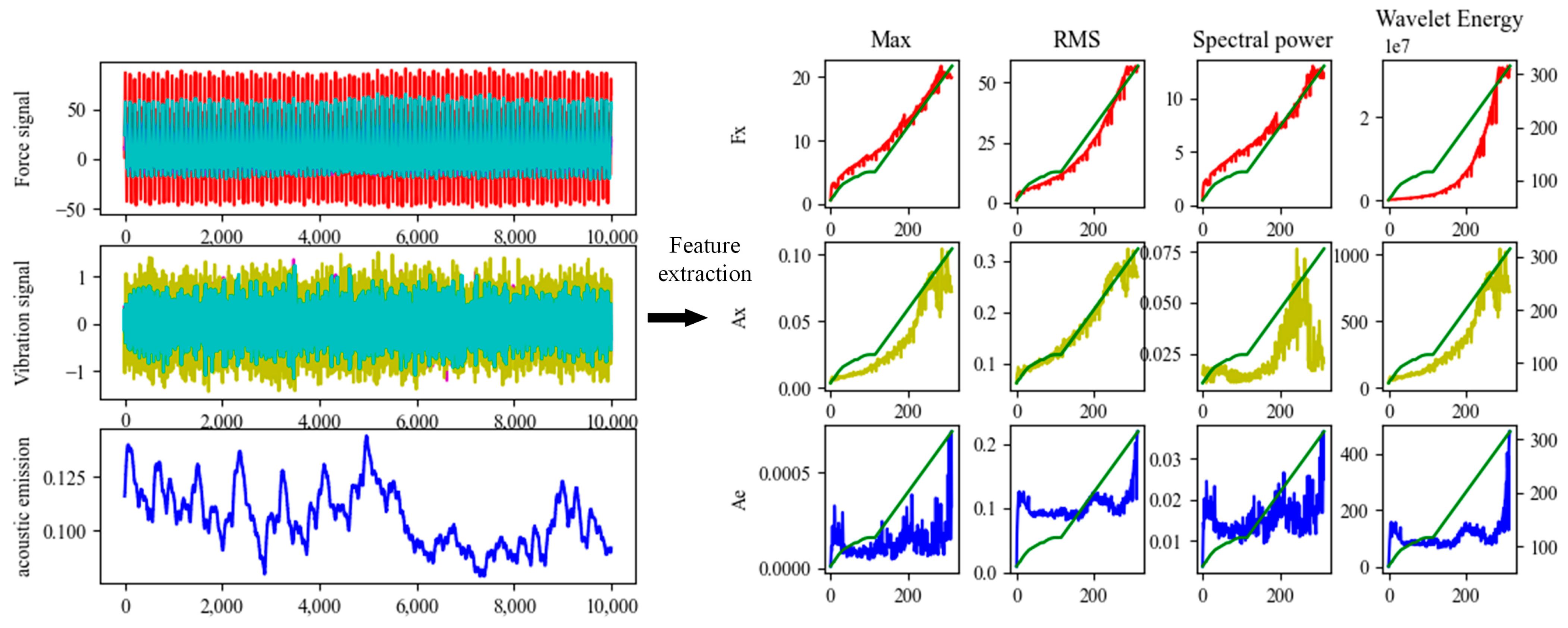
Feature selection is a data preprocessing technique to reduce the dimensions of the inputs of the prediction model. The reduction of input features reduces the complexity of the deep learning model, thus reducing the time for model training and testing and to avoid having too few features in the training samples, resulting in insufficient fitting of the prediction model. As shown in Figure 12, the force signals in three directions, vibration signals in three directions, and acoustic emission signals are shown in different colors in the left side of the figure. 12 features were extracted from them and compared with the correlation of tool wear. and compared with the correlation of tool wear. After correlation analysis, 10 features were selected, as shown in Table 1.

Figure 12.
Feature extraction for seven signal channels.

Table 1.
List of extracted features.
4.3. Model Training
The datasets C1, C4, and C6 were processed according to the chosen preprocessing method and then randomly divided into training, testing, and validation sets. The model was trained using the training set, while the testing and validation sets were used to evaluate the model’s performance. Table 2 provides a detailed description of the experimental datasets.

Table 2.
Settings of training and testing sets.
The proposed model was trained on an RTX1060 GPU (NVDIA, Santa Clara, CA, USA) with 6 GB memory. The optimizer was set as Adam, the training epochs were set as 600 with batch size 20, and the initial learning rate was set as 0.001. The mean squared error was used as the loss function and the Adam optimizer was selected to update the model parameters. To avoid overfitting, this study applied L2 regularization during the training process to improve the generalization ability of model. The loss function with regularization was as follows:
where and are the predicted and the true wear at the t moment, respectively, represents the weight of the regularization term .
5. Results and Discussion
5.1. Evaluation Metrics
To evaluate the performance of the model, the mean absolute error (MAE), root mean square error (RMSE) and mean absolute percentage error (MAPE) were employed for evaluation. MAE describes the proximity between the estimation and actual tool wear values, while RMSE magnifies actual errors to provide a clearer picture of predictive accuracy. The expressions are as follows:
5.2. Performance of the DResNet-1d Model for Tool Condition Monitoring
To assess the effectiveness and superiority of the DResNet-1d model, some common models were used to make a comparison using the same datasets. All models are listed as follows:
SVR: traditional machine learning model based on support vector regression;
1D-CNN: deep learning model based on one-dimensional convolutional neural network;
BiLSTM: a variant of RNN, with two LSTMs in opposite directions;
BiGRU: a variant of parameter simplification of a LSTM network, with two GRUs in opposite directions.
To make the comparison between the five models more fairly, the main parameters were consistent, and a series of unified settings was adopted. For example, the optimizer was Adam, the dropout rate was 0.5, and the loss function was MSE.
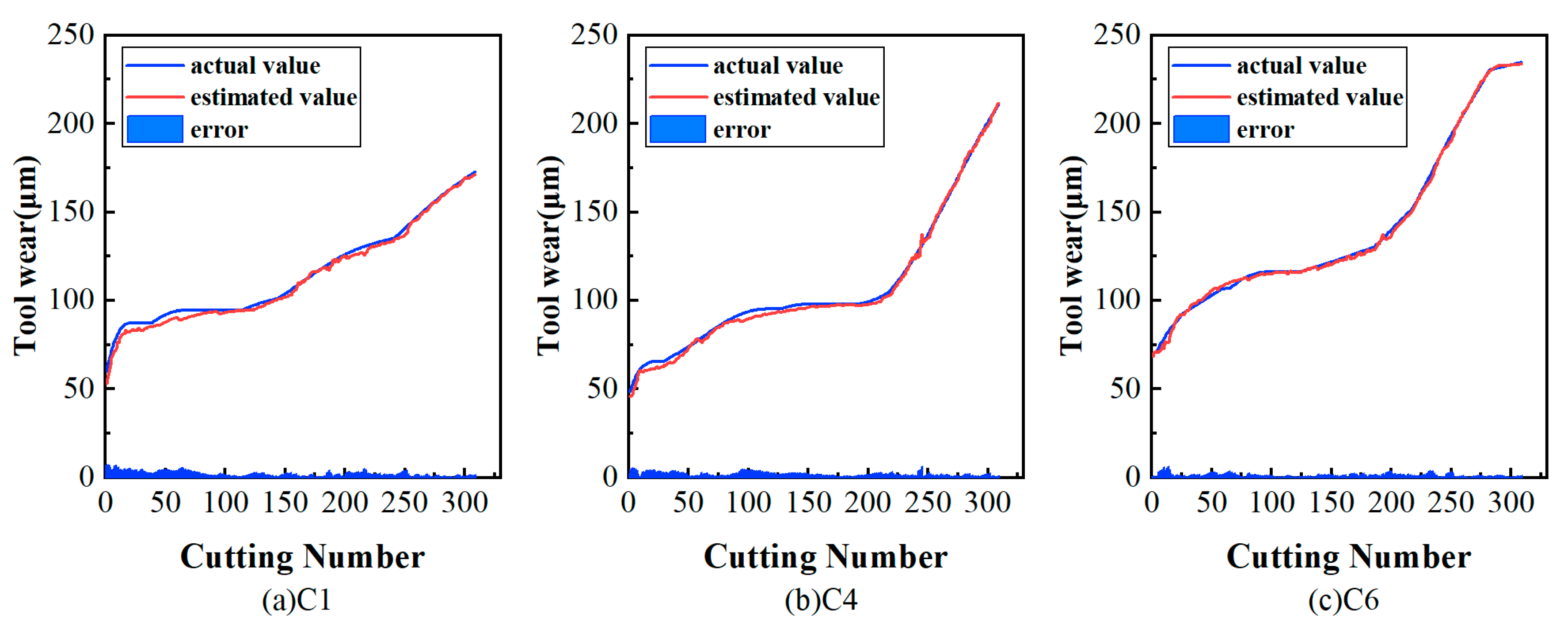
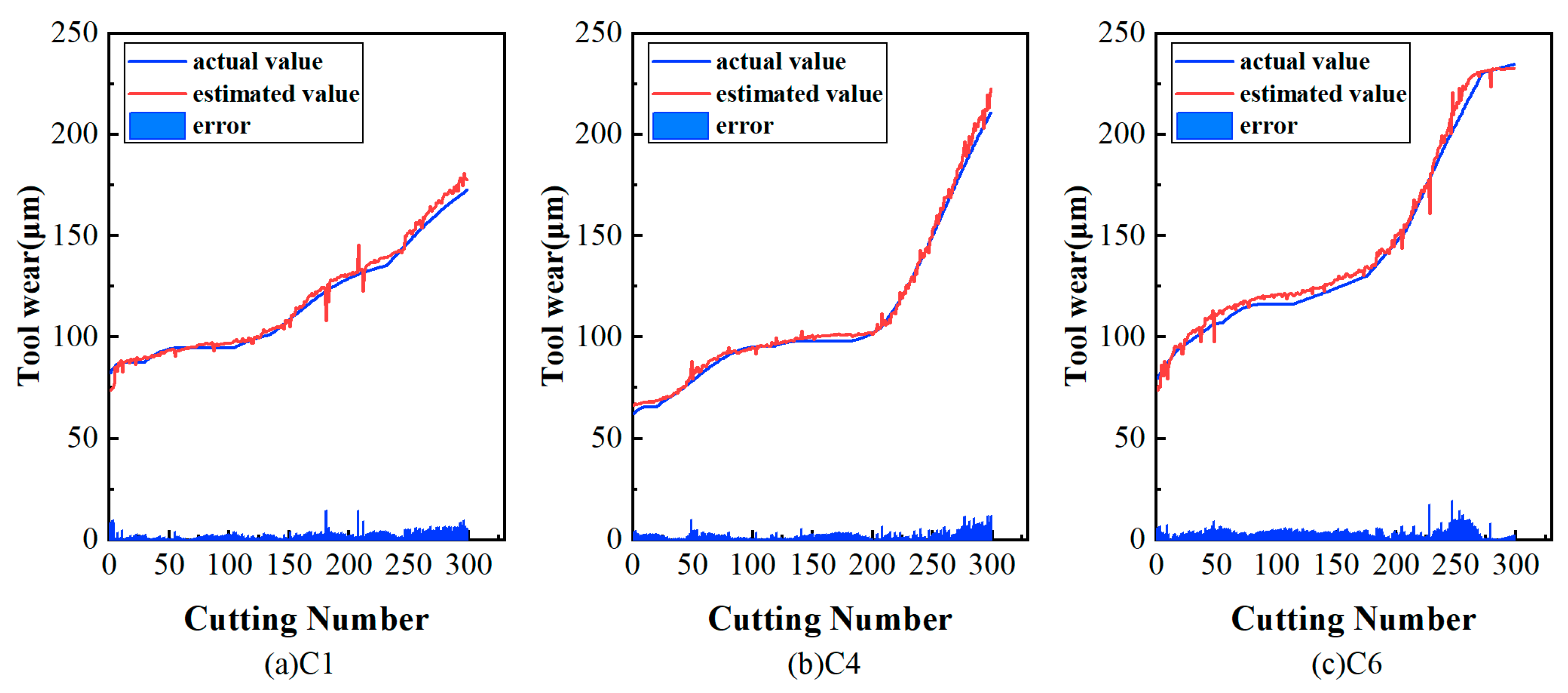
The validation results of C1 are presented in Figure 13. The evaluation metrics for each model are listed in Table 3. Comparing the validation results of models, deep learning models outperformed traditional machine learning models. Within the realm of deep learning methods, the mean RMSE and MAE values of the DResNet-1d model were 3.09 and 2.28, respectively, which stand out in comparison to the results of other models. This indicates the incorporation of residual connections in the CNN mitigates issues such as gradient vanishing and network degradation. This allows for the efficient extraction of specific features and simplification of spatial information within the signal and exhibits remarkable feature extraction capabilities and abstract learning abilities.
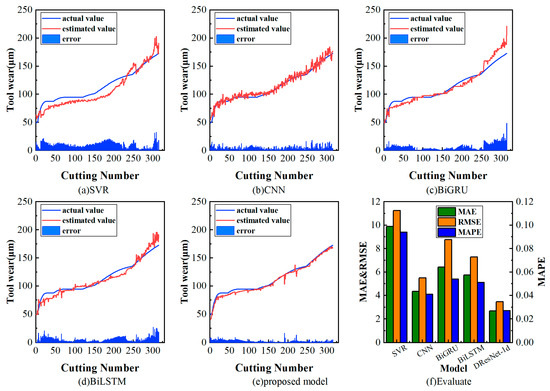
Figure 13.
Tool wear estimation results for the PHM dataset.

Table 3.
Performance of different models for the PHM dataset.
5.3. Effectiveness of Smoothing Correction for Tool Condition Monitoring
It can be observed from the results of the monitoring that there were inevitably local fluctuations and outliers in the wear curve of each model, which affected the total accuracy. To improve the accuracy of estimation results, it is possible to improve the structure of the model, or to correct the estimation to reduce local fluctuations in the curve.
Some traditional algorithms have been used for time-series smoothing, such as moving average models, and autoregressive differential moving average models. Considering the latency and performance of the model, triple exponential smoothing can be chosen [37].
The encoder- and decoder-based temporal model was used to perform smoothing correction on the estimation. The comparison of evaluation results after correction using the temporal model and the triple exponential smoothing algorithms are shown in Figure 14, and the MAE and RMSE are listed in Table 4.
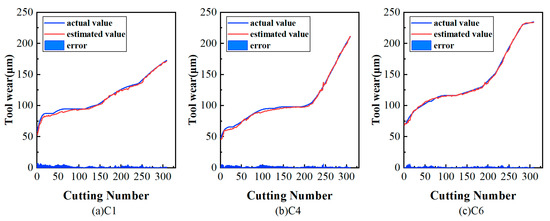
Figure 14.
Results of temporal model smoothing for the PHM dataset.

Table 4.
Performance of smoothing algorithm for the PHM dataset.
The experimental results demonstrated that both methods showed a good performance, reducing local fluctuations in adjacent time step ranges while retaining the trend of the wear curve, making the estimated tool wear values more stable. In contrast, although the triple exponential smoothing method was relatively simple, its overall smoothing effect was inferior to that of the encoder- and decoder-based temporal model.
5.4. Performance of Tool Wear Prediction Model on Multi-Step Prediction
Similar to the smoothing process, the tool wear prediction model took as inputs multiple consecutive historical tool wear values estimated by the DResNet-1d model and computed predicted future tool wear values. It established a mapping relationship between historical tool wear information and future tool wear values. For this paper, short-term and long-term predictions were performed and tool wear values were predicted for each dataset at 5, 10, and 15 moments in the future, respectively. The results of the five-step prediction are shown in Figure 15. To validate the performance of the proposed model, the results were obtained by comparing them with those of standard deep learning models (CNN and GRU) and advanced deep learning models (Transformer and SMAML). All the results are shown in Table 5.
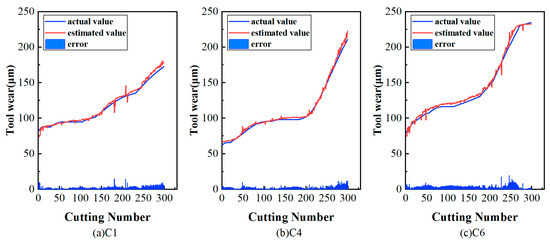
Figure 15.
Five-step prediction results of the proposed method for the PHM dataset.

Table 5.
The prediction results of 5 steps, 10 steps, and 15 steps for the PHM dataset.
From the analysis of the experimental results listed in Table 5, the results of the proposed prediction model outperformed the basic deep learning model and the advanced deep learning model on multi-step prediction, which proved that the model can learn the short-term features and long-term trends of time information. Meanwhile, the RMSE and MAE of 5, 10, and 15 steps showed an increasing trend, indicating a higher accuracy in the short-term prediction compared to the long-term prediction.
5.5. Validation of Generalization Capability of the Tool Wear Prediction Model
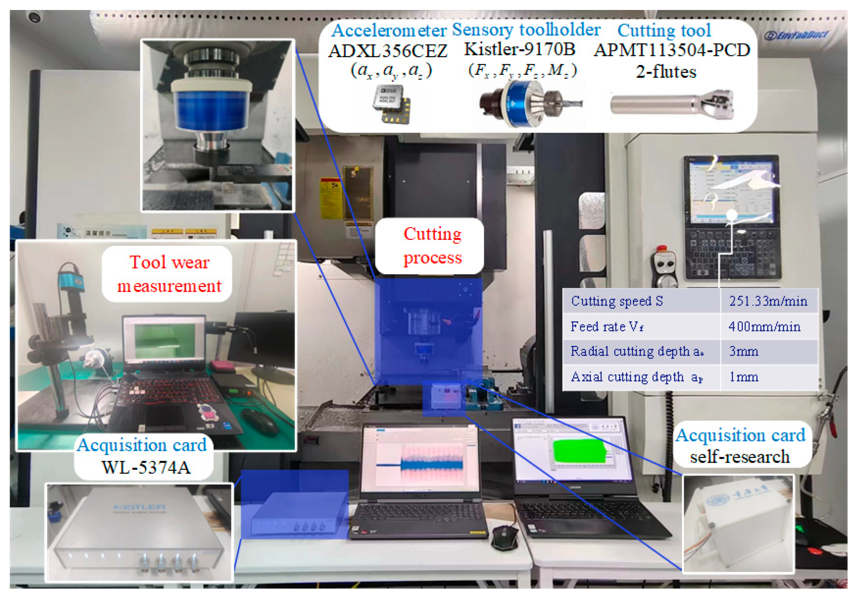
The proposed tool wear prediction method was applied to the machining of carbon fiber-reinforced polymer (CFRP) to test its generalization in a real machining environment. Side milling experiments were conducted on a three-axis vertical machining center (VMC855) in a dry cutting environment. The workpiece material was CFRP, the size was 450 mm × 40 mm × 11 mm, and the milling cutter was equipped with one APMT1135 PCD insert with a cutting diameter of 20 mm ( specific process parameters are shown in Table 6).

Table 6.
CFRP milling test parameters.
As shown in Figure 16, the force acquisition system collected the three-axis cutting force signals Fx, Fy, Fz, and the Z-axis bending moment Mz, respectively. It consisted of a wireless rotary dynamometer (Kistler-9170B), a wireless transmission module, and display software (PTS App Type Z22059-900). The sampling frequency was 2.5 kHz. The acceleration acquisition system consisted of a wireless rotation dynamometer (Kistler-9170B) and a wireless transmission module with a sampling frequency of 2.5 kHz. The acceleration acquisition system consisted of a self-developed ADXL356CEZ three-way capacitive acceleration sensor, a wireless acquisition board, and visualization software (self-developed) from Chongqing University. The accelerometer was attached to the surface of the workpiece with adhesive and the sampling frequency was 10 kHz.
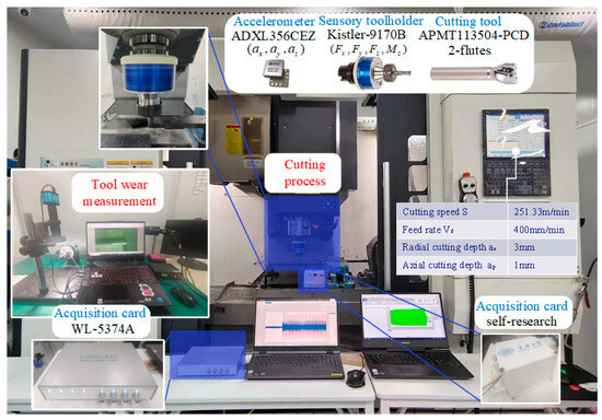
Figure 16.
The CFRP milling experiments setup.
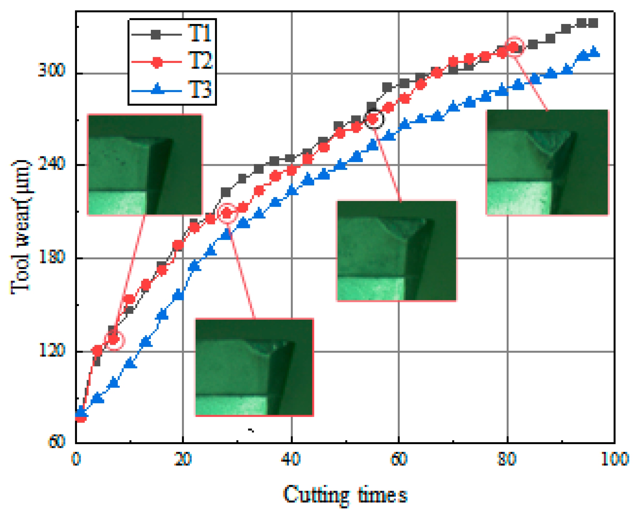
Three single-tooth tools were used for multiple milling experiments of CFRP components. Taking a wear value of 300 um as the criterion for tool failure, each tool was milled approximately 80–100 times. Three datasets consisting of cutting signals and wear values were obtained, i.e., T1, T2, and T3. In order to minimize the measurement errors, a digital microscope (MV-HM2000GM) was used to collect the tool wear images after each cutting experiment without disassembling the inserts, and the corresponding tool wear values were measured. The tool life for one set of experiments is shown in Figure 17, where the width of the flank wear increased significantly with the number of cuts.

Figure 17.
Tool wear of T1, T2, and T3.
Multi-domain feature extraction was performed on signals from six channels (cutting force and cutting vibration in three vertical directions). Figure 18 illustrates the signal features under three sets of experiments and differentiates the different features with colors. Then, ten features described in Table 1 were selected from each experiment.

Figure 18.
Multi-domain sensor signal feature extraction results for tools T1, T2, and T3.
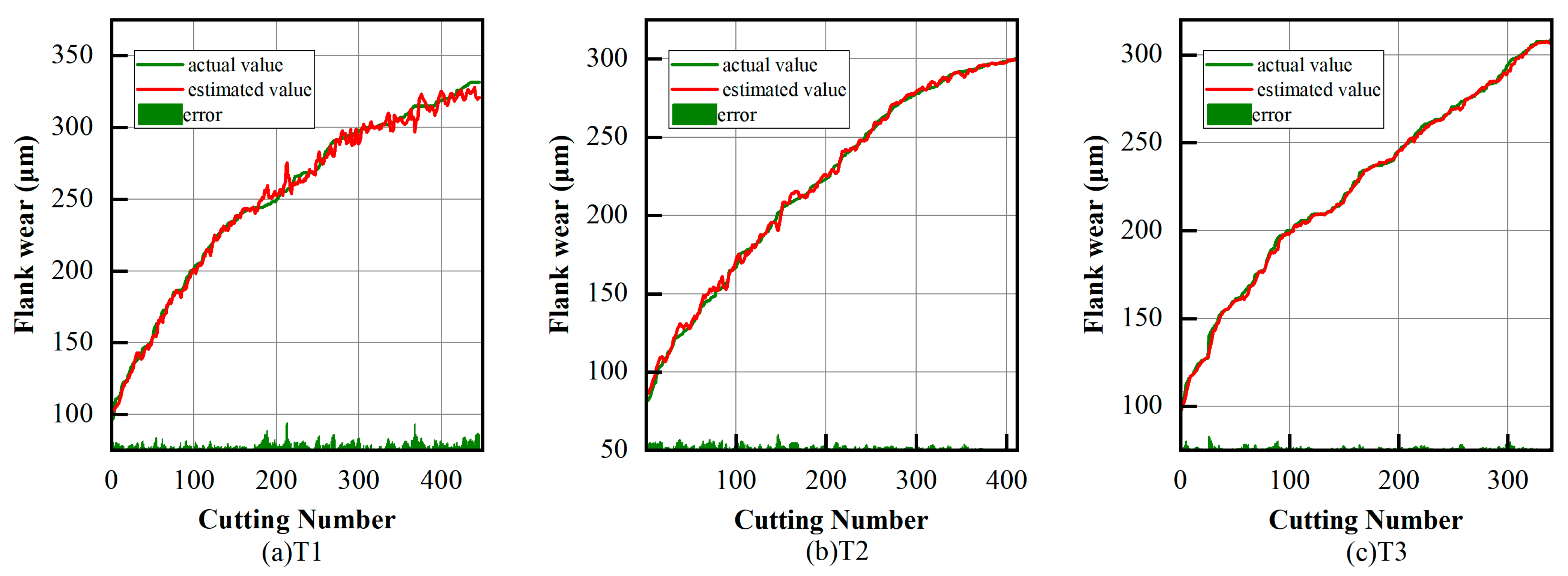
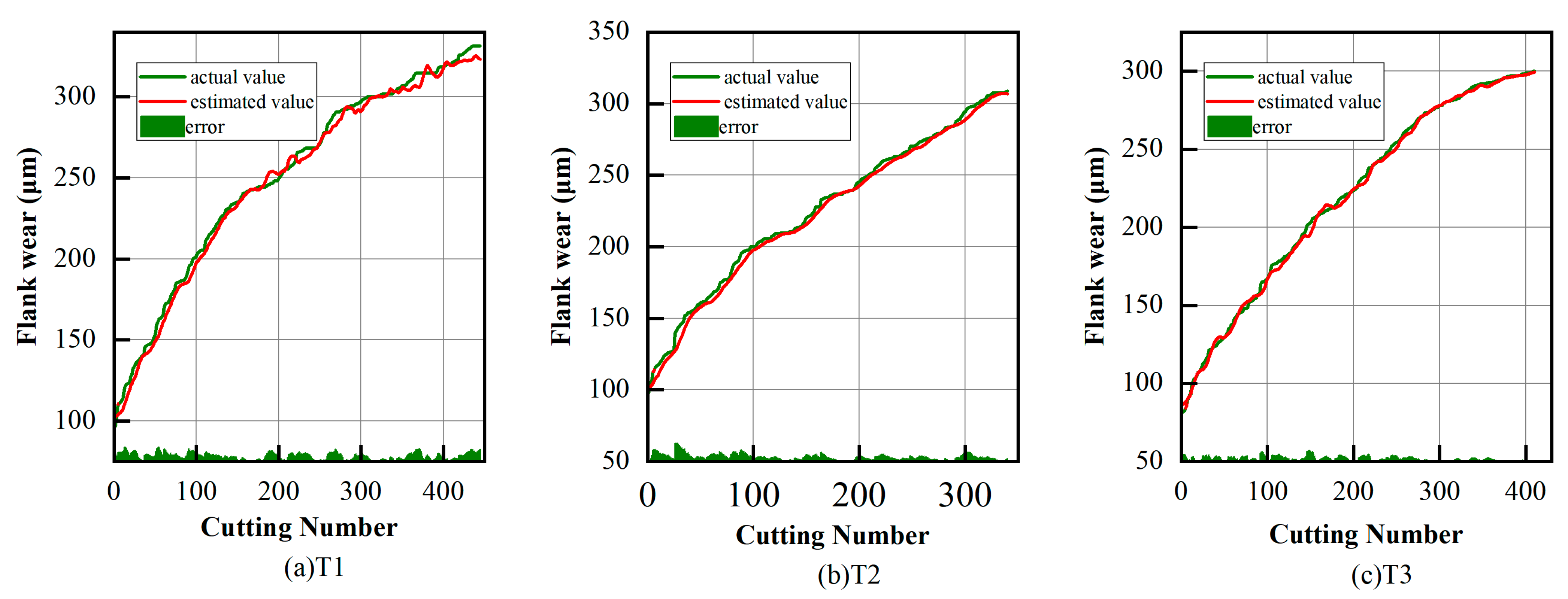
The extracted features were input into the monitoring and prediction model to verify model accuracy. Figure 19 and Figure 20 show the predicted results of flank wear in the three tool experiments. Specific results are shown in Table 7 and Table 8. The prediction results show that the proposed model was able to accurately realize tool wear monitoring and prediction during milling of CFRP workpieces, proving the generalization ability of the model to learn other machining conditions.
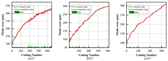
Figure 19.
Tool wear estimation results.
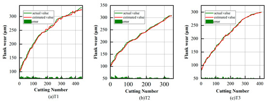
Figure 20.
Five-step prediction results of proposed method.

Table 7.
Performance of proposed models on tool wear estimation.

Table 8.
The prediction results of 5 steps, 10 steps, and 15 steps.
6. Conclusions
In this research, an integrated system that can be used for online tool wear monitoring and prediction was designed, and its effectiveness was verified with a publicly available dataset and experiments. The conclusions are summarized as follows:
- (1)
- A DResNet-1d model based on 1d residual structure was proposed to extract deep features of multi-source information in which gradient vanishing and model degradation are alleviated. BN layers and dropout are used in the model to improve the generalization ability of the model and avoid overfitting. The model showed superiority in various indicators.
- (2)
- An encoder- and decoder-based temporal model was proposed to capture time dependency, and an attention mechanism was introduced to improve the generalization capacity of the model. To reduce the local fluctuation and outliers, the encoder and decoder-based temporal model was used to perform smoothing correction. The average RMSE of tool wear estimation was significantly reduced to 2.1 after correcting.
- (3)
- To give early warning of tool conditions, the temporal model was used to predict tool wear values in future moments. In our experiments, the next 5, 10, and 15 steps of tool wear values were predicted, showing a good performance. This proved that the model can learn the short-term features and long-term trends of temporal information.
Author Contributions
Conceptualization, Z.L. and X.L.; methodology, Z.L.; software, X.L.; validation, X.L., Z.Y. and H.L.; formal analysis, T.H.; investigation, H.L.; resources, D.L.; data curation, Z.Y.; writing—original draft preparation, Z.L.; writing—review and editing, X.L.; visualization, Z.L.; supervision, K.G.; project administration, D.L.; funding acquisition, D.L. All authors have read and agreed to the published version of the manuscript.
Funding
This research was funded in part by the National Key Research and Development Program of China (2022YFB3206700), in part by the Open fund for the National Key Laboratory of Intelligent Manufacturing Equipment and Technology (Grant No. IMETKF2024004).
Data Availability Statement
Experimental data were obtained from the Prognostics and Health Management Society 2010 PHM Society Conference Data Challenge. The resource can be found in the corresponding reference.
Conflicts of Interest
Author Zhichao You was employed by the company The Leading Optics (Shanghai) Company, Ltd. The remaining authors declare that the research was conducted in the absence of any commercial or financial relationships that could be construed as a potential conflict of interest.
References
- Wang, J.; Xu, C.; Zhang, J.; Zhong, R. Big data analytics for intelligent manufacturing systems: A review. J. Manuf. Syst. 2022, 62, 738–752. [Google Scholar] [CrossRef]
- Liao, X.; Zhou, G.; Zhang, Z.; Lu, J.; Ma, J. Tool wear state recognition based on GWO–SVM with feature selection of genetic algorithm. Int. J. Adv. Manuf. Technol. 2019, 104, 1051–1063. [Google Scholar] [CrossRef]
- Aghazadeh, F.; Tahan, A.; Thomas, M. Tool condition monitoring using spectral subtraction and convolutional neural networks in milling process. Int. J. Adv. Manuf. Technol. 2018, 98, 3217–3227. [Google Scholar] [CrossRef]
- Li, H.N.; Xie, K.G.; Wu, B.; Zhu, W.Q. Generation of textured diamond abrasive tools by continuous-wave CO2 laser: Laser parameter effects and optimisation. J. Mater. Process. Technol. 2020, 275, 116279. [Google Scholar] [CrossRef]
- Liu, C.; Li, Y.; Hua, J.; Lu, N.; Mou, W. Real-time cutting tool state recognition approach based on machining features in NC machining process of complex structural parts. Int. J. Adv. Manuf. Technol. 2018, 97, 229–241. [Google Scholar] [CrossRef]
- Kong, D.; Chen, Y.; Li, N. Gaussian process regression for tool wear prediction. Mech. Syst. Signal Process. 2018, 104, 556–574. [Google Scholar] [CrossRef]
- You, Z.; Gao, H.; Li, S.; Guo, L.; Liu, Y.; Li, J. Multiple Activation Functions and Data Augmentation-Based Lightweight Network for In Situ Tool Condition Monitoring. IEEE Trans. Ind. Electron. 2022, 69, 13656–13664. [Google Scholar] [CrossRef]
- You, Z.; Meng, Y.; Li, D.; Zhang, Z.; Ren, M.; Zhang, X.; Zhu, L. Adaptive detection of tool-workpiece contact for nanoscale tool setting based on multi-scale decomposition of force signal. Mech. Syst. Signal Process. 2024, 208, 111000. [Google Scholar] [CrossRef]
- Bouhalais, M.L.; Nouioua, M. The analysis of tool vibration signals by spectral kurtosis and ICEEMDAN modes energy for insert wear monitoring in turning operation. Int. J. Adv. Manuf. Technol. 2021, 115, 2989–3001. [Google Scholar] [CrossRef]
- Yen, C.L.; Lu, M.C.; Chen, J.L. Applying the self-organization feature map (SOM) algorithm to AE-based tool wear monitoring in micro-cutting. Mech. Syst. Signal Process. 2013, 34, 353–366. [Google Scholar] [CrossRef]
- da Silva, R.H.L.; da Silva, M.B.; Hassui, A. A probabilistic neural network applied in monitoring tool wear in the end milling operation via acoustic emission and cutting power signals. Mach. Sci. Technol. 2016, 20, 386–405. [Google Scholar] [CrossRef]
- Sun, M.; Guo, K.; Zhang, D.; Yang, B.; Sun, J.; Li, D.; Huang, T. A novel exponential model for tool remaining useful life prediction. J. Manuf. Syst. 2024, 73, 223–240. [Google Scholar] [CrossRef]
- Wang, J.; Li, Y.; Zhao, R.; Gao, R.X. Physics guided neural network for machining tool wear prediction. J. Manuf. Syst. 2020, 57, 298–310. [Google Scholar] [CrossRef]
- Li, Y.; Wang, J.; Huang, Z.; Gao, R.X. Physics-informed meta learning for machining tool wear prediction. J. Manuf. Syst. 2022, 62, 17–27. [Google Scholar] [CrossRef]
- Liao, Z.R.; Li, S.M.; Lu, Y.; Gao, D. Tool wear Identification in turning titanium alloy based on SVM. In Materials Science Forum; Trans Tech Publications Ltd.: Bäch SZ, Switzerland, 2014; pp. 446–450. [Google Scholar]
- Li, W.; Liu, T. Time varying and condition adaptive hidden Markov model for tool wear state estimation and remaining useful life prediction in micro-milling. Mech. Syst. Signal Process. 2019, 131, 689–702. [Google Scholar] [CrossRef]
- Chen, J.C.; Chen, J.C. An artificial-neural-networks-based in-process tool wear prediction system in milling operations. Int. J. Adv. Manuf. Technol. 2005, 25, 427–434. [Google Scholar] [CrossRef]
- Cheng, M.; Jiao, L.; Shi, X.; Wang, X.; Yan, P.; Li, Y. An intelligent prediction model of the tool wear based on machine learning in turning high strength steel. Proc. Inst. Mech. Eng. Part B J. Eng. Manuf. 2020, 234, 1580–1597. [Google Scholar] [CrossRef]
- Wang, J.; Wang, P.; Gao, R.X. Enhanced particle filter for tool wear prediction. J. Manuf. Syst. 2015, 36, 35–45. [Google Scholar] [CrossRef]
- Han, S.; Mannan, N.; Stein, D.C.; Pattipati, K.R.; Bollas, G.M. Classification and regression models of audio and vibration signals for machine state monitoring in precision machining systems. J. Manuf. Syst. 2021, 61, 45–53. [Google Scholar] [CrossRef]
- Xu, X.; Wang, J.; Zhong, B.; Ming, W.; Chen, M. Deep learning-based tool wear prediction and its application for machining process using multi-scale feature fusion and channel attention mechanism. Measurement 2021, 177, 109254. [Google Scholar] [CrossRef]
- Duan, J.; Duan, J.; Zhou, H.; Zhan, X.; Li, T.; Shi, T. Multi-frequency-band deep CNN model for tool wear prediction. Meas. Sci. Technol. 2021, 32, 065009. [Google Scholar] [CrossRef]
- Yin, Y.; Wang, S.; Zhou, J. Multisensor-based tool wear diagnosis using 1D-CNN and DGCCA. Appl. Intell. 2023, 53, 4448–4461. [Google Scholar] [CrossRef]
- Shah, M.; Vakharia, V.; Chaudhari, R.; Vora, J.; Pimenov, D.Y.; Giasin, K. Tool wear prediction in face milling of stainless steel using singular generative adversarial network and LSTM deep learning models. Int. J. Adv. Manuf. Technol. 2022, 121, 723–736. [Google Scholar] [CrossRef]
- Wu, X.; Li, J.; Jin, Y.; Zheng, S. Modeling and analysis of tool wear prediction based on SVD and BiLSTM. Int. J. Adv. Manuf. Technol. 2020, 106, 4391–4399. [Google Scholar] [CrossRef]
- Zhang, N.; Chen, E.; Wu, Y.; Guo, B.; Jiang, Z.; Wu, F. A novel hybrid model integrating residual structure and bi-directional long short-term memory network for tool wear monitoring. Int. J. Adv. Manuf. Technol. 2022, 120, 6707–6722. [Google Scholar] [CrossRef]
- Xu, X.; Tao, Z.; Ming, W.; An, Q.; Chen, M. Intelligent monitoring and diagnostics using a novel integrated model based on deep learning and multi-sensor feature fusion. Measurement 2020, 165, 108086. [Google Scholar] [CrossRef]
- Gu, J.; Wang, Z.; Kuen, J.; Ma, L.; Shahroudy, A.; Shuai, B.; Liu, T.; Wang, X.; Wang, G.; Cai, J.; et al. Recent advances in convolutional neural networks. Pattern Recognit. 2018, 77, 354–377. [Google Scholar] [CrossRef]
- Krizhevsky, A.; Sutskever, I.; Hinton, G.E. Imagenet classification with deep convolutional neural networks. Adv. Neural Inf. Process. Syst. 2017, 60, 84–90. [Google Scholar] [CrossRef]
- He, K.; Zhang, X.; Ren, S.; Sun, J. Deep residual learning for image recognition. In Proceedings of the IEEE Conference on Computer Vision and Pattern Recognition, Las Vegas, NV, USA, 27–30 June 2016; pp. 770–778. [Google Scholar]
- Chung, J.; Gulcehre, C.; Cho, K.; Bengio, Y. Empirical evaluation of gated recurrent neural networks on sequence modeling. arXiv 2014, arXiv:1412.3555. [Google Scholar]
- Sutskever, I.; Vinyals, O.; Le, Q.V. Sequence to sequence learning with neural networks. Adv. Neural Inf. Process. Syst. 2014, 27. [Google Scholar]
- Vaswani, A.; Shazeer, N.; Parmar, N.; Uszkoreit, J.; Jones, L.; Gomez, A.N.; Kaiser, Ł.; Polosukhin, I. Attention is all you need. Adv. Neural Inf. Process. Syst. 2017, 30. [Google Scholar]
- He, K.; Zhang, X.; Ren, S.; Sun, J. Identity mappings in deep residual networks. In Proceedings of the Computer Vision–ECCV 2016: 14th European Conference, Amsterdam, The Netherlands, 11–14 October 2016; Part IV 14. pp. 630–645. [Google Scholar]
- Chen, Y.; Jin, Y.; Jiri, G. Predicting tool wear with multi-sensor data using deep belief networks. Int. J. Adv. Manuf. Technol. 2018, 99, 1917–1926. [Google Scholar] [CrossRef]
- Li, Y.; Xie, Q.; Huang, H.; Chen, Q. Research on a tool wear monitoring algorithm based on residual dense network. Symmetry 2019, 11, 809. [Google Scholar] [CrossRef]
- Liu, X.; Liu, S.; Li, X.; Zhang, B.; Yue, C.; Liang, S.Y. Intelligent tool wear monitoring based on parallel residual and stacked bidirectional long short-term memory network. J. Manuf. Syst. 2021, 60, 608–619. [Google Scholar] [CrossRef]
- Wu, N.; Green, B.; Ben, X.; O’Banion, S. Deep transformer models for time series forecasting: The influenza prevalence case. arXiv 2020, arXiv:2001.08317. [Google Scholar]
- Wang, G.; Zhang, F. A sequence-to-sequence model with attention and monotonicity loss for tool wear monitoring and prediction. IEEE Trans. Instrum. Meas. 2021, 70, 3525611. [Google Scholar] [CrossRef]
Disclaimer/Publisher’s Note: The statements, opinions and data contained in all publications are solely those of the individual author(s) and contributor(s) and not of MDPI and/or the editor(s). MDPI and/or the editor(s) disclaim responsibility for any injury to people or property resulting from any ideas, methods, instructions or products referred to in the content. |
© 2024 by the authors. Licensee MDPI, Basel, Switzerland. This article is an open access article distributed under the terms and conditions of the Creative Commons Attribution (CC BY) license (https://creativecommons.org/licenses/by/4.0/).

