
Predicting Machine Failures from Multivariate Time Series: An Industrial Case Study


Abstract
1. Introduction
- We compare three ML methods (logistic regression, random forest, and Support Vector Machine) and three DL methods (LSTM, ConvLSTM, and Transformer) on three novel industrial datasets with multiple telemetry data.
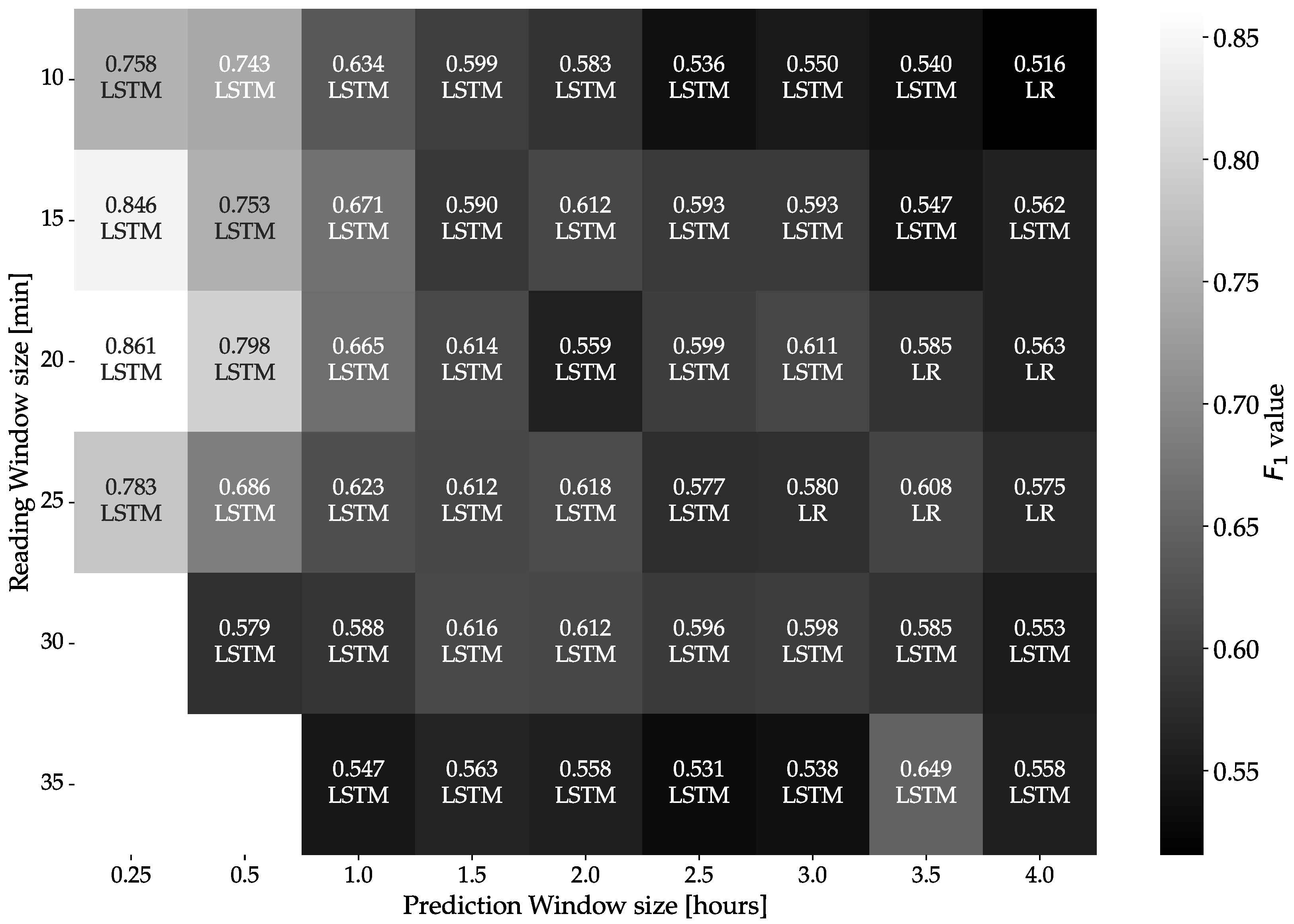
- We study the effect of varying the size of both the reading window and the prediction window in the context of failure prediction and discuss the consequences of these choices on the performances.
- We define and evaluate the diversity of patterns preceding faults and the datasets’ complexities, showing that DL approaches outperform ML approaches significantly only for complex datasets with more diverse patterns.
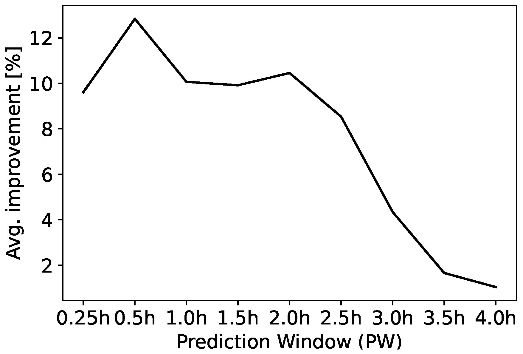
- We show that all methods lose predictive power when the horizon enlarges because the temporal correlation between the input and the predicted event tends to vanish.
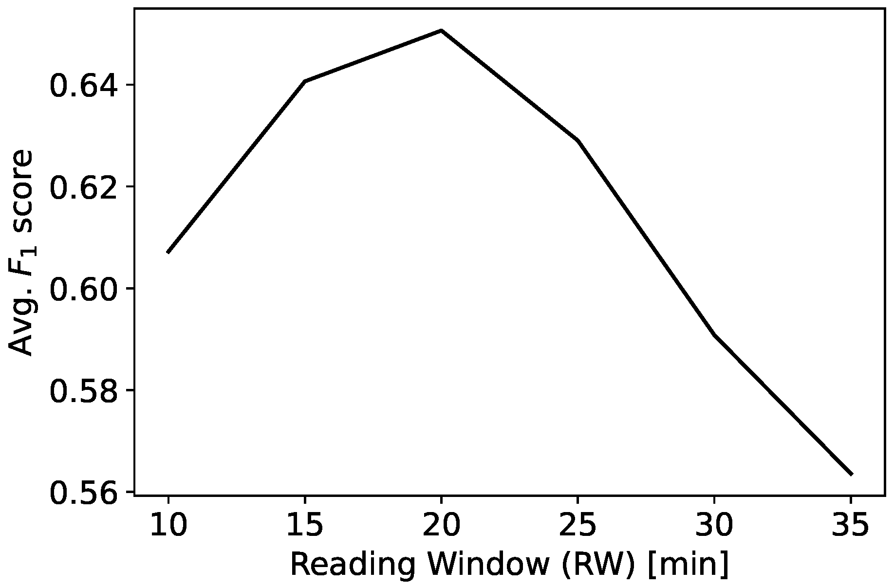
- We highlight that when patterns are diverse, the amount of historical data becomes influential. However, augmenting the amount of input is not beneficial in general.
- We publish the datasets and the compared algorithms (available at https://github.com/nicolopinci/polimi_failure_prediction (accessed on 19 May 2024)). The published datasets are among the few publicly accessible by researchers in the domain of fault prediction for industrial machines [27].
2. Related Work
3. Materials and Methods
3.1. Datasets
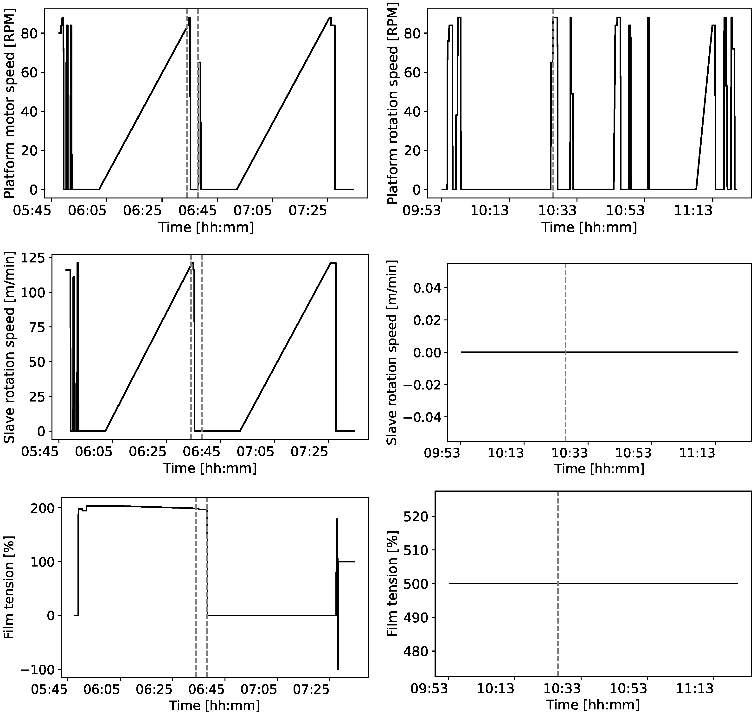
3.1.1. Wrapping Machine
- Loading the products on a pallet at the centre of the rotating platform.
- Tying the film’s trailing end to the pallet’s base.
- Starting the wrapping cycle, executed according to previously set parameters.
- Manually cutting the film (through the cutter or with an external tool) and making it adhere to the wrapped products.
- Removing the wrapped objects.
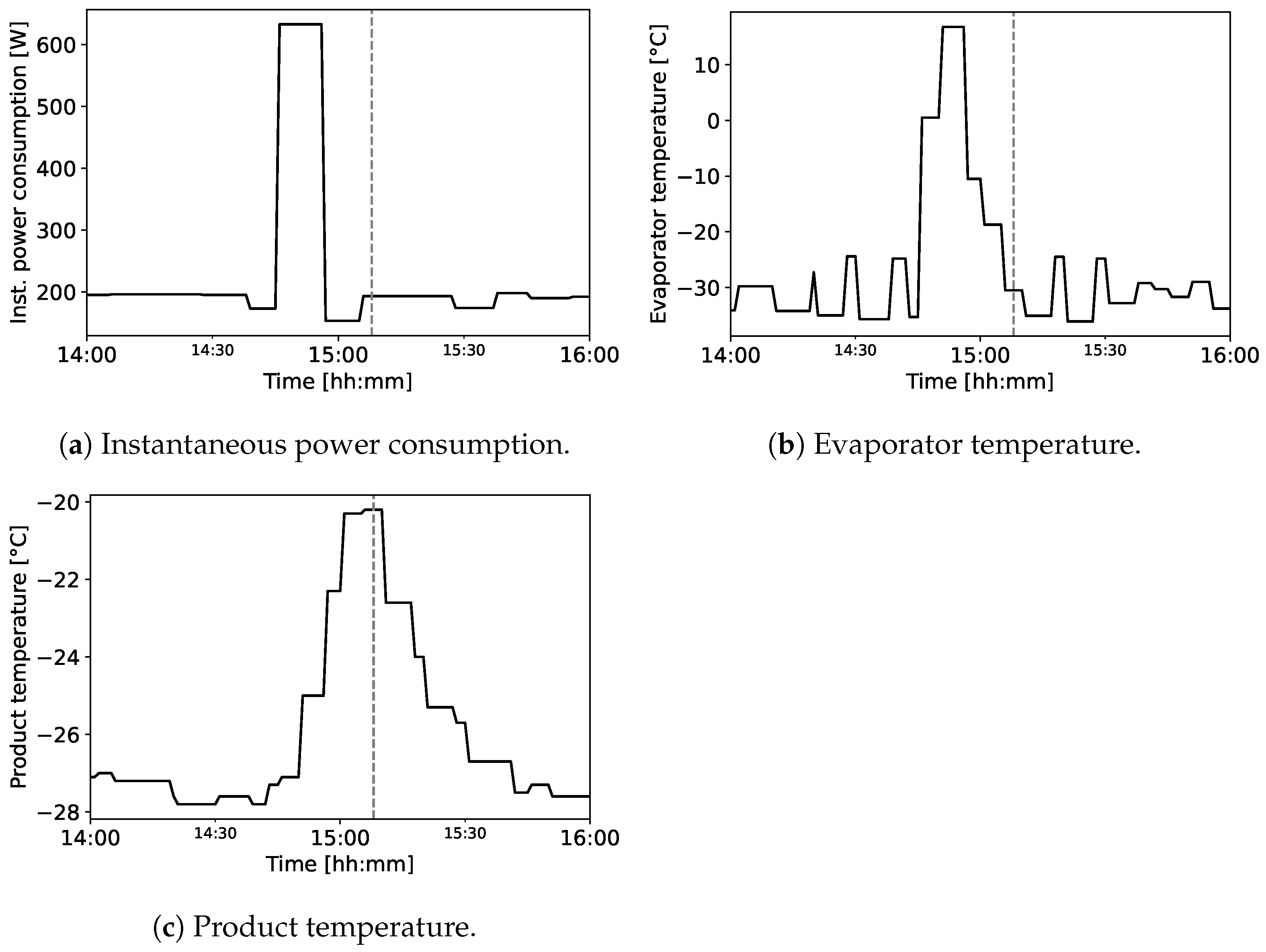
3.1.2. Blood Refrigerator
- Compression: The cycle begins with the compressor drawing in low-pressure, low-temperature refrigerant gas. The compressor then compresses the gas, which raises its pressure and temperature.
- Condensation: The high-pressure, high-temperature gas exits the compressor and enters the condenser coils. As the gas flows through these coils, it releases heat, cools down, and condenses into a high-pressure liquid.
- Expansion: This high-pressure liquid then flows through the capillary tube or expansion valve. As it does, its pressure drops, causing a significant drop in temperature. The refrigerant exits this stage as a low-pressure, cool liquid.
- Evaporation: The low-pressure, cool liquid refrigerant enters the evaporator coils inside the refrigerator. Here, it absorbs heat from the interior, causing it to evaporate and turn back into a low-pressure gas. This process cools the interior of the refrigerator.
- Return to Compressor: The low-pressure gas then returns to the compressor and the cycle starts over.
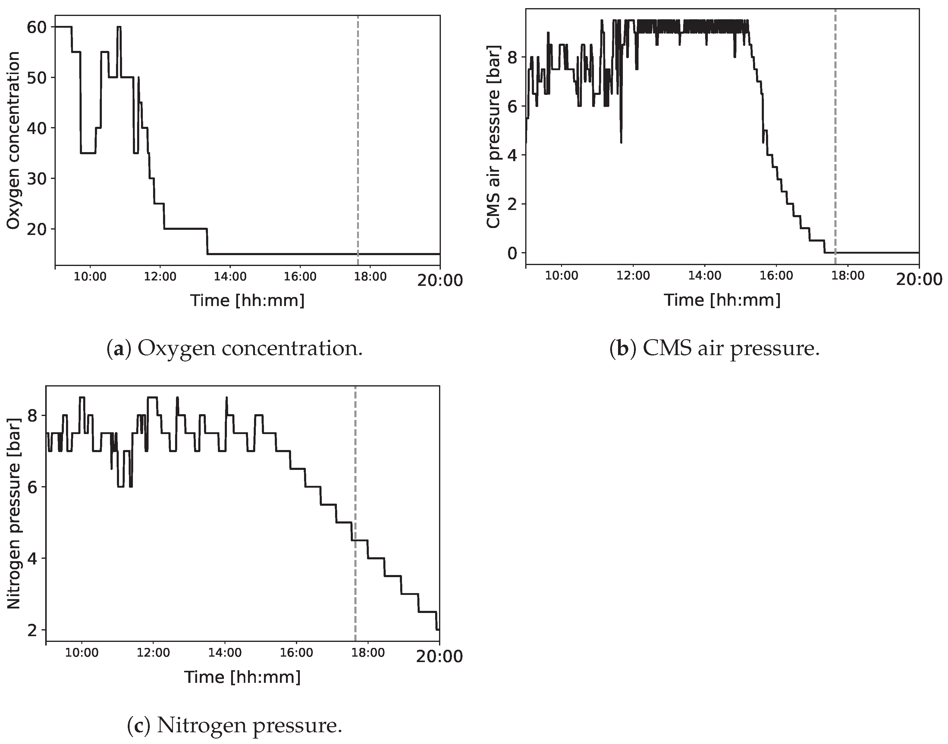
3.1.3. Nitrogen Generator
- The air compressor compresses the air to a high pressure and supplies it to the machine.
- In the towers, the CMS adsorbs smaller gas molecules, such as oxygen, while allowing larger nitrogen molecules to pass through the sieve and go into the vessels.
- The buffer tank receives the nitrogen gas from the vessels through the valves.
- The valves reduce the pressure in the current working tower to release the residual gasses, whereas in the other towers, the pressure is increased to restart the process.
3.2. Data Processing
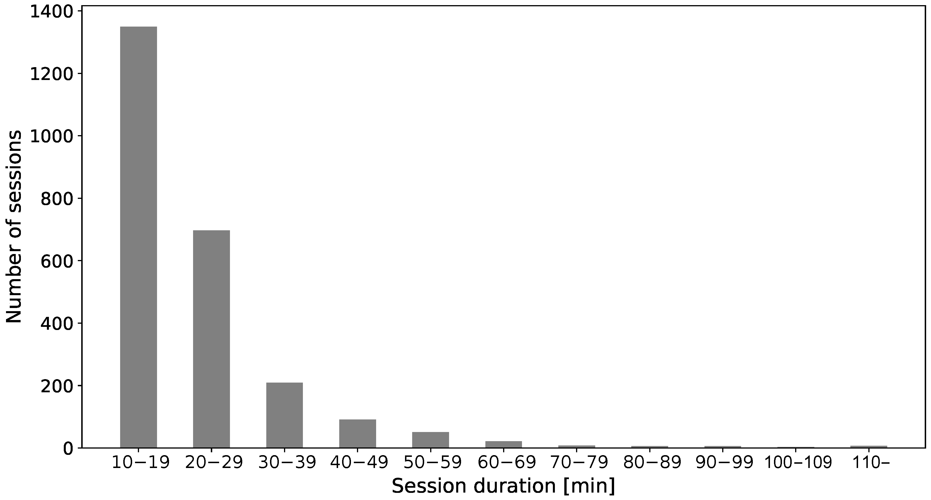
3.2.1. Wrapping Machine
| Algorithm 1 Computation of session boundaries |
| Require: , the dataset containing, for each timestamp, an array with the values of the movement variables, structured as a hash map with the timestamp as the key and the movement variables array as the value Ensure: , a map that associates a session number to each timestamp and −1 to out-of-session timestamps 1: 2: false 3: 4: 5: for do 6: 7: if then 8: 9: 10: if then 11: 12: true 13: 14: else 15: if true then 16: 17: if min then 18: 19: false 20: end if 21: end if 22: end if 23: else 24: 25: end if 26: end for |
3.2.2. Blood Refrigerator
3.2.3. Nitrogen Generator
3.3. Definition of the Reading and Prediction Windows
3.4. Class Unbalance
3.5. Algorithms and Hyperparameter Tuning
3.6. Training and Evaluation
- For each k-fold split, the data are divided into a train set , comprising the folds with , and a test set , corresponding to .
- For each and , RUS is applied to balance the classes, obtaining 10 RUS instances for the test set and 10 RUS instances for the train set.
- For each , the six presented algorithms , with their hyperparameters , are trained on the train folds and evaluated on the RUS instance on the test fold, obtaining macro scores on the test set, denoted as .
- For each algorithm and hyperparameter setting, the mean of the results is computed as .
- Then, the maximum macro score for each algorithm is computed as .
- Finally, the best macro score is computed as , and the best algorithm as .
4. Results
4.1. Wrapping Machine
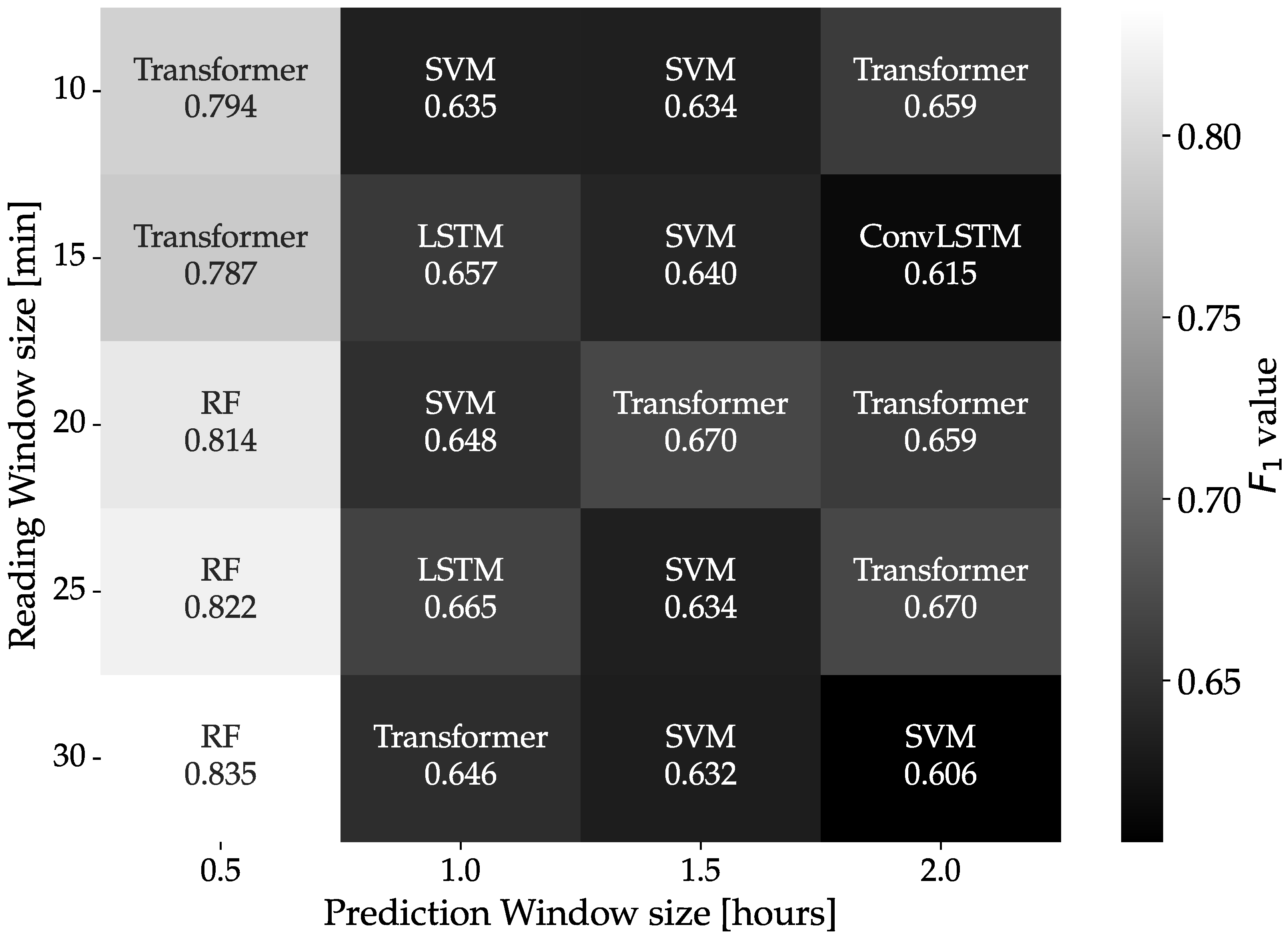
4.2. Blood Refrigerator
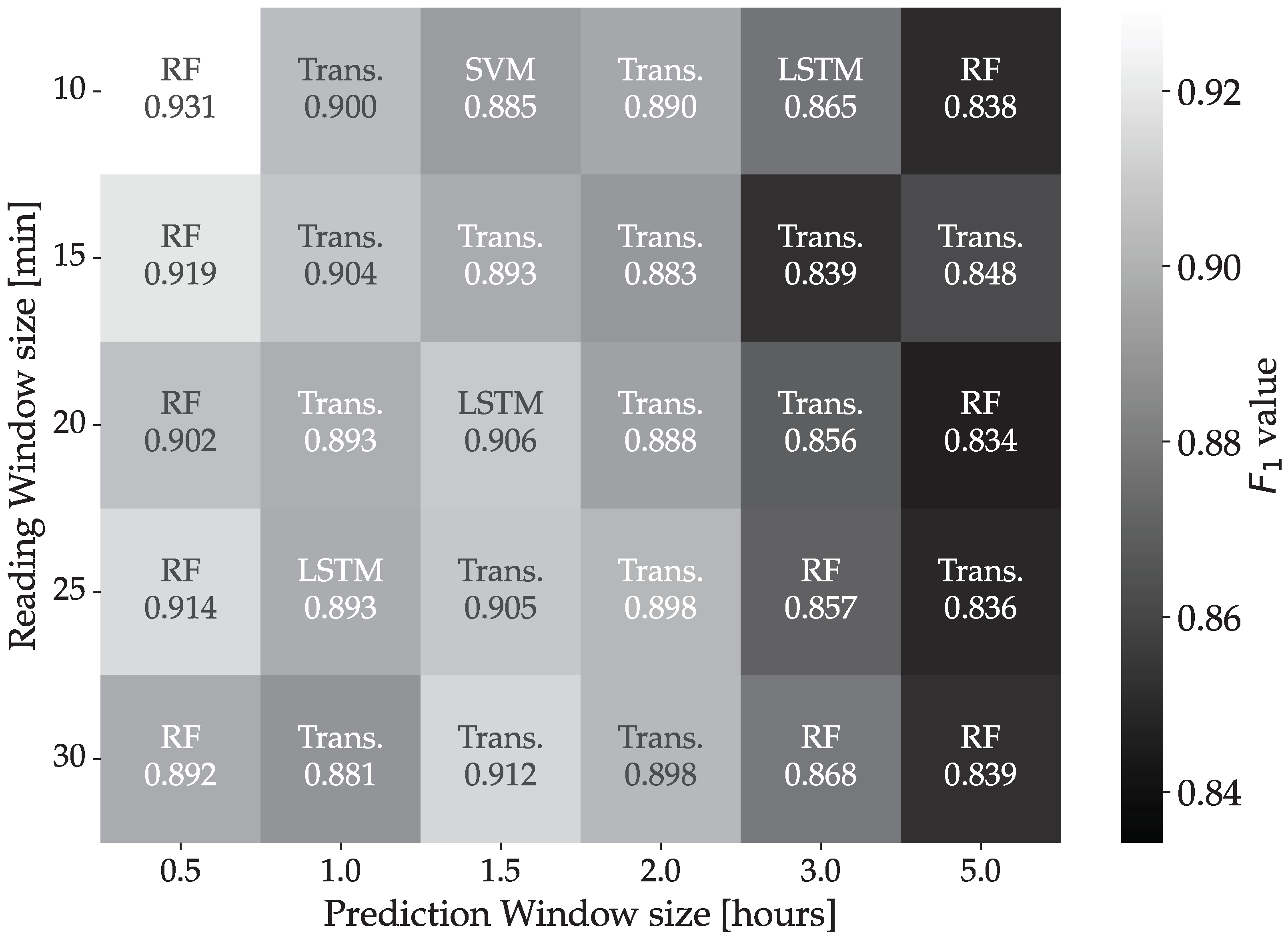
4.3. Nitrogen Generator
4.4. Execution Time
5. Conclusions
Author Contributions
Funding
Data Availability Statement
Conflicts of Interest
References
- Bousdekis, A.; Apostolou, D.; Mentzas, G. Predictive Maintenance in the 4th Industrial Revolution: Benefits, Business Opportunities, and Managerial Implications. IEEE Eng. Manag. Rev. 2020, 48, 57–62. [Google Scholar] [CrossRef]
- Zonta, T.; da Costa, C.A.; da Rosa Righi, R.; de Lima, M.J.; da Trindade, E.S.; Li, G.P. Predictive maintenance in the Industry 4.0: A systematic literature review. Comput. Ind. Eng. 2020, 150, 106889. [Google Scholar] [CrossRef]
- Dalzochio, J.; Kunst, R.; Pignaton, E.; Binotto, A.; Sanyal, S.; Favilla, J.; Barbosa, J. Machine learning and reasoning for predictive maintenance in Industry 4.0: Current status and challenges. Comput. Ind. 2020, 123, 103298. [Google Scholar] [CrossRef]
- Sheut, C.; Krajewski, L.J. A decision model for corrective maintenance management. Int. J. Prod. Res. 1994, 32, 1365–1382. [Google Scholar] [CrossRef]
- Wang, Y.; Deng, C.; Wu, J.; Wang, Y.; Xiong, Y. A corrective maintenance scheme for engineering equipment. Eng. Fail. Anal. 2014, 36, 269–283. [Google Scholar] [CrossRef]
- Meller, R.D.; Kim, D.S. The impact of preventive maintenance on system cost and buffer size. Eur. J. Oper. Res. 1996, 95, 577–591. [Google Scholar] [CrossRef]
- Wu, S.; Zuo, M. Linear and Nonlinear Preventive Maintenance Models. IEEE Trans. Reliab. 2010, 59, 242–249. [Google Scholar] [CrossRef]
- Liang, H.; Song, L.; Wang, J.; Guo, L.; Li, X.; Liang, J. Robust unsupervised anomaly detection via multi-time scale DCGANs with forgetting mechanism for industrial multivariate time series. Neurocomputing 2021, 423, 444–462. [Google Scholar] [CrossRef]
- Tian, Z.; Zhuo, M.; Liu, L.; Chen, J.; Zhou, S. Anomaly detection using spatial and temporal information in multivariate time series. Sci. Rep. 2023, 13, 4400. [Google Scholar] [CrossRef]
- Salfner, F.; Lenk, M.; Malek, M. A survey of online failure prediction methods. ACM Comput. Surv. 2010, 42, 1–42. [Google Scholar] [CrossRef]
- García, F.P.; Pedregal, D.J.; Roberts, C. Time series methods applied to failure prediction and detection. Reliab. Eng. Syst. Saf. 2010, 95, 698–703. [Google Scholar] [CrossRef]
- Leukel, J.; González, J.; Riekert, M. Machine learning-based failure prediction in industrial maintenance: Improving performance by sliding window selection. Int. J. Qual. Reliab. Manag. 2022, 40, 1449–1462. [Google Scholar] [CrossRef]
- Box, G.; Jenkins, G.M. Time Series Analysis: Forecasting and Control; Wiley: Hoboken, NJ, USA, 2016. [Google Scholar]
- Łuczak, D.; Brock, S.; Siembab, K. Cloud Based Fault Diagnosis by Convolutional Neural Network as Time–Frequency RGB Image Recognition of Industrial Machine Vibration with Internet of Things Connectivity. Sensors 2023, 23, 3755. [Google Scholar] [CrossRef] [PubMed]
- Pertselakis, M.; Lampathaki, F.; Petrali, P. Predictive Maintenance in a Digital Factory Shop-Floor: Data Mining on Historical and Operational Data Coming from Manufacturers’ Information Systems. In Lecture Notes in Business Information Processing; Springer International Publishing: Berlin/Heidelberg, Germany, 2019; pp. 120–131. [Google Scholar] [CrossRef]
- Khorsheed, R.M.; Beyca, O.F. An integrated machine learning: Utility theory framework for real-time predictive maintenance in pumping systems. Proc. Inst. Mech. Eng. Part B J. Eng. Manuf. 2020, 235, 887–901. [Google Scholar] [CrossRef]
- Proto, S.; Ventura, F.; Apiletti, D.; Cerquitelli, T.; Baralis, E.; Macii, E.; Macii, A. PREMISES, a Scalable Data-Driven Service to Predict Alarms in Slowly-Degrading Multi-Cycle Industrial Processes. In Proceedings of the 2019 IEEE International Congress on Big Data (BigDataCongress), Milan, Italy, 8–13 July 2019. [Google Scholar] [CrossRef]
- Kaparthi, S.; Bumblauskas, D. Designing predictive maintenance systems using decision tree-based machine learning techniques. Int. J. Qual. Reliab. Manag. 2020, 37, 659–686. [Google Scholar] [CrossRef]
- Alves, F.; Badikyan, H.; Moreira, H.A.; Azevedo, J.; Moreira, P.M.; Romero, L.; Leitao, P. Deployment of a Smart and Predictive Maintenance System in an Industrial Case Study. In Proceedings of the 2020 IEEE 29th International Symposium on Industrial Electronics (ISIE), Delft, The Netherlands, 17–19 June 2020. [Google Scholar] [CrossRef]
- Dix, M.; Chouhan, A.; Sinha, M.; Singh, A.; Bhattarai, S.; Narkhede, S.; Prabhune, A. An AI-based Alarm Prediction in Industrial Process Control Systems. In Proceedings of the 2022 IEEE International Conference on Big Data and Smart Computing (BigComp), Daegu, Republic of Korea, 17–20 January 2022. [Google Scholar] [CrossRef]
- Colone, L.; Dimitrov, N.; Straub, D. Predictive repair scheduling of wind turbine drive-train components based on machine learning. Wind Energy 2019, 22, 17–19. [Google Scholar] [CrossRef]
- Leahy, K.; Gallagher, C.; O’Donovan, P.; Bruton, K.; O’Sullivan, D. A Robust Prescriptive Framework and Performance Metric for Diagnosing and Predicting Wind Turbine Faults Based on SCADA and Alarms Data with Case Study. Energies 2018, 11, 1738. [Google Scholar] [CrossRef]
- Bonnevay, S.; Cugliari, J.; Granger, V. Predictive Maintenance from Event Logs Using Wavelet-Based Features: An Industrial Application. In Advances in Intelligent Systems and Computing; Springer International Publishing: Berlin/Heidelberg, Germany, 2019; pp. 132–141. [Google Scholar] [CrossRef]
- Barraza, J.F.; Bräuning, L.G.; Perez, R.B.; Morais, C.B.; Martins, M.R.; Droguett, E.L. Deep learning health state prognostics of physical assets in the Oil and Gas industry. Proc. Inst. Mech. Eng. Part O: J. Risk Reliab. 2020, 236, 598–616. [Google Scholar] [CrossRef]
- Kusiak, A.; Verma, A. A Data-Mining Approach to Monitoring Wind Turbines. IEEE Trans. Sustain. Energy 2012, 3, 150–157. [Google Scholar] [CrossRef]
- Li, H.; Parikh, D.; He, Q.; Qian, B.; Li, Z.; Fang, D.; Hampapur, A. Improving rail network velocity: A machine learning approach to predictive maintenance. Transp. Res. Part C Emerg. Technol. 2014, 45, 17–26. [Google Scholar] [CrossRef]
- Forbicini, F.; Pinciroli Vago, N.O.; Fraternali, P. Time Series Analysis in Compressor-Based Machines: A Survey. arXiv 2024, arXiv:2402.17802. [Google Scholar] [CrossRef]
- Laptev, N.; Amizadeh, S.; Flint, I. Generic and Scalable Framework for Automated Time-series Anomaly Detection. In Proceedings of the 21th ACM SIGKDD International Conference on Knowledge Discovery and Data Mining, Sydney, Australia, 10–13 August 2015. [Google Scholar] [CrossRef]
- Ren, H.; Xu, B.; Wang, Y.; Yi, C.; Huang, C.; Kou, X.; Xing, T.; Yang, M.; Tong, J.; Zhang, Q. Time-Series Anomaly Detection Service at Microsoft. In Proceedings of the 25th ACM SIGKDD International Conference on Knowledge Discovery & Data Mining, Sydney, Australia, 10–13 August 2015. [Google Scholar] [CrossRef]
- Chen, K.; Pashami, S.; Fan, Y.; Nowaczyk, S. Predicting Air Compressor Failures Using Long Short Term Memory Networks. In Progress in Artificial Intelligence; Springer International Publishing: Berlin/Heidelberg, Germany, 2019; pp. 596–609. [Google Scholar] [CrossRef]
- Leukel, J.; González, J.; Riekert, M. Adoption of machine learning technology for failure prediction in industrial maintenance: A systematic review. J. Manuf. Syst. 2021, 61, 87–96. [Google Scholar] [CrossRef]
- Zangrando, N.; Fraternali, P.; Petri, M.; Pinciroli Vago, N.O.; González, S.L.H. Anomaly detection in quasi-periodic energy consumption data series: A comparison of algorithms. Energy Inform. 2022, 5, 62. [Google Scholar] [CrossRef]
- Carrera, D.; Manganini, F.; Boracchi, G.; Lanzarone, E. Defect Detection in SEM Images of Nanofibrous Materials. IEEE Trans. Ind. Inform. 2017, 13, 551–561. [Google Scholar] [CrossRef]
- Si, W.; Yang, Q.; Wu, X. Material Degradation Modeling and Failure Prediction Using Microstructure Images. Technometrics 2018, 61, 246–258. [Google Scholar] [CrossRef]
- Bionda, A.; Frittoli, L.; Boracchi, G. Deep Autoencoders for Anomaly Detection in Textured Images Using CW-SSIM. In Image Analysis and Processing – ICIAP 2022; Springer International Publishing: Berlin/Heidelberg, Germany, 2022; pp. 669–680. [Google Scholar] [CrossRef]
- Xue, Z.; Dong, X.; Ma, S.; Dong, W. A Survey on Failure Prediction of Large-Scale Server Clusters. In Proceedings of the Eighth ACIS International Conference on Software Engineering, Artificial Intelligence, Networking, and Parallel/Distributed Computing (SNPD 2007), Qingdao, China, 30 July–1 August 2007. [Google Scholar] [CrossRef]
- Ramezani, S.B.; Killen, B.; Cummins, L.; Rahimi, S.; Amirlatifi, A.; Seale, M. A Survey of HMM-based Algorithms in Machinery Fault Prediction. In Proceedings of the 2021 IEEE Symposium Series on Computational Intelligence (SSCI), Orlando, FL, USA, 5–7 December 2021. [Google Scholar] [CrossRef]
- Yoon, A.S.; Lee, T.; Lim, Y.; Jung, D.; Kang, P.; Kim, D.; Park, K.; Choi, Y. Semi-supervised Learning with Deep Generative Models for Asset Failure Prediction. arXiv 2017, arXiv:1709.00845. [Google Scholar] [CrossRef]
- Zhao, M.; Furuhata, R.; Agung, M.; Takizawa, H.; Soma, T. Failure Prediction in Datacenters Using Unsupervised Multimodal Anomaly Detection. In Proceedings of the 2020 IEEE International Conference on Big Data (Big Data), Atlanta, GA, USA, 10–13 December 2020. [Google Scholar] [CrossRef]
- Nowaczyk, S.; Prytz, R.; Rögnvaldsson, T.; Byttner, S. Towards a machine learning algorithm for predicting truck compressor failures using logged vehicle data. In Proceedings of the 12th Scandinavian Conference on Artificial Intelligence, Aalborg, Denmark, 20–22 November 2013; IOS Press: Amsterdam, The Netherlands, 2013; pp. 205–214. [Google Scholar]
- Prytz, R.; Nowaczyk, S.; Rögnvaldsson, T.; Byttner, S. Predicting the need for vehicle compressor repairs using maintenance records and logged vehicle data. Eng. Appl. Artif. Intell. 2015, 41, 139–150. [Google Scholar] [CrossRef]
- Canizo, M.; Onieva, E.; Conde, A.; Charramendieta, S.; Trujillo, S. Real-time predictive maintenance for wind turbines using Big Data frameworks. In Proceedings of the 2017 IEEE International Conference on Prognostics and Health Management (ICPHM), Dallas, TX, USA, 19–21 June 2017. [Google Scholar] [CrossRef]
- Xiang, S.; Huang, D.; Li, X. A Generalized Predictive Framework for Data Driven Prognostics and Diagnostics using Machine Logs. In Proceedings of the TENCON 2018 - 2018 IEEE Region 10 Conference, Jeju, Republic of Korea, 28–31 October 2018. [Google Scholar] [CrossRef]
- Mishra, K.; Manjhi, S.K. Failure Prediction Model for Predictive Maintenance. In Proceedings of the 2018 IEEE International Conference on Cloud Computing in Emerging Markets (CCEM), Bangalore, India, 23–24 November 2018. [Google Scholar] [CrossRef]
- Kulkarni, K.; Devi, U.; Sirighee, A.; Hazra, J.; Rao, P. Predictive Maintenance for Supermarket Refrigeration Systems Using Only Case Temperature Data. In Proceedings of the 2018 Annual American Control Conference (ACC), Milwaukee, WI, USA, 27–29 June 2018. [Google Scholar] [CrossRef]
- Susto, G.A.; Schirru, A.; Pampuri, S.; McLoone, S.; Beghi, A. Machine Learning for Predictive Maintenance: A Multiple Classifier Approach. IEEE Trans. Ind. Inform. 2015, 11, 812–820. [Google Scholar] [CrossRef]
- Hamaide, V.; Glineur, F. Predictive Maintenance of a Rotating Condenser Inside a Synchrocyclotron. In Proceedings of the 28th Belgian Dutch Conference on Machine Learning (Benelearn 2019), Brussels, Belgium, 6–8 November 2019. [Google Scholar]
- Orrù, P.F.; Zoccheddu, A.; Sassu, L.; Mattia, C.; Cozza, R.; Arena, S. Machine Learning Approach Using MLP and SVM Algorithms for the Fault Prediction of a Centrifugal Pump in the Oil and Gas Industry. Sustainability 2020, 12, 4776. [Google Scholar] [CrossRef]
- Yu, Y.; Si, X.; Hu, C.; Zhang, J. A Review of Recurrent Neural Networks: LSTM Cells and Network Architectures. Neural Comput. 2019, 31, 1235–1270. [Google Scholar] [CrossRef]
- Fagerström, J.; Bång, M.; Wilhelms, D.; Chew, M.S. LiSep LSTM: A Machine Learning Algorithm for Early Detection of Septic Shock. Sci. Rep. 2019, 9, 15132. [Google Scholar] [CrossRef]
- Aung, N.N.; Pang, J.; Chua, M.C.H.; Tan, H.X. A novel bidirectional LSTM deep learning approach for COVID-19 forecasting. Sci. Rep. 2023, 13. [Google Scholar] [CrossRef] [PubMed]
- Jin, L.; Wenbo, H.; You, J.; Lei, W.; Fei, J. A ConvLSTM-Based Approach to Wind Turbine Gearbox Condition Prediction. In Proceedings of the 7th PURPLE MOUNTAIN FORUM on Smart Grid Protection and Control (PMF2022); Springer Nature Singapore: Singapore, 2023; pp. 529–545. [Google Scholar] [CrossRef]
- Alos, A.; Dahrouj, Z. Using MLSTM and Multioutput Convolutional LSTM Algorithms for Detecting Anomalous Patterns in Streamed Data of Unmanned Aerial Vehicles. IEEE Aerosp. Electron. Syst. Mag. 2022, 37, 6–15. [Google Scholar] [CrossRef]
- Shi, X.; Chen, Z.; Wang, H.; Yeung, D.Y.; Wong, W.K.; WOO, W.C. Convolutional LSTM Network: A Machine Learning Approach for Precipitation Nowcasting. In Proceedings of the Advances in Neural Information Processing Systems; Cortes, C., Lawrence, N., Lee, D., Sugiyama, M., Garnett, R., Eds.; Curran Associates, Inc.: Scotland, UK, 2015; Volume 28. [Google Scholar]
- Szarek, D.; Jabłoński, I.; Zimroz, R.; Wyłomańska, A. Non-Gaussian feature distribution forecasting based on ConvLSTM neural network and its application to robust machine condition prognosis. Expert Syst. Appl. 2023, 230, 120588. [Google Scholar] [CrossRef]
- Wu, X.; Geng, J.; Liu, M.; Song, Z.; Song, H. Prediction of Node Importance of Power System Based on ConvLSTM. Energies 2022, 15, 3678. [Google Scholar] [CrossRef]
- Tuli, S.; Casale, G.; Jennings, N.R. TranAD: Deep Transformer Networks for Anomaly Detection in Multivariate Time Series Data. arXiv 2022, arXiv:2201.07284. [Google Scholar] [CrossRef]
- Huang, S.; Liu, Y.; Fung, C.; He, R.; Zhao, Y.; Yang, H.; Luan, Z. HitAnomaly: Hierarchical Transformers for Anomaly Detection in System Log. IEEE Trans. Netw. Serv. Manag. 2020, 17, 2064–2076. [Google Scholar] [CrossRef]
- Jin, Y.; Hou, L.; Chen, Y. A Time Series Transformer based method for the rotating machinery fault diagnosis. Neurocomputing 2022, 494, 379–395. [Google Scholar] [CrossRef]
- Wu, B.; Cai, W.; Cheng, F.; Chen, H. Simultaneous-fault diagnosis considering time series with a deep learning transformer architecture for air handling units. Energy Build. 2022, 257, 111608. [Google Scholar] [CrossRef]
- Gao, P.; Guan, L.; Hao, J.; Chen, Q.; Yang, Y.; Qu, Z.; Jin, M. Fault Prediction in Electric Power Communication Network Based on Improved DenseNet. In Proceedings of the 2023 IEEE International Symposium on Broadband Multimedia Systems and Broadcasting (BMSB), Beijing, China, 14–16 June 2023. [Google Scholar] [CrossRef]
- Tang, L.; Lv, H.; Yang, F.; Yu, L. Complexity testing techniques for time series data: A comprehensive literature review. Chaos Solitons Fractals 2015, 81, 117–135. [Google Scholar] [CrossRef]
- Inouye, T.; Shinosaki, K.; Sakamoto, H.; Toi, S.; Ukai, S.; Iyama, A.; Katsuda, Y.; Hirano, M. Quantification of EEG irregularity by use of the entropy of the power spectrum. Electroencephalogr. Clin. Neurophysiol. 1991, 79, 204–210. [Google Scholar] [CrossRef]
- Saxena, S.; Odono, V.; Uba, J.; Nelson, J.M.; Lewis, W.L.; Shulman, I.A. The Risk of Bacterial Growth in Units of Blood that Have Warmed to More Than 10 °C. Am. J. Clin. Pathol. 1990, 94, 80–83. [Google Scholar] [CrossRef] [PubMed]
- Blaine, K.P.; Cortés-Puch, I.; Sun, J.; Wang, D.; Solomon, S.B.; Feng, J.; Gladwin, M.T.; Kim-Shapiro, D.B.; Basu, S.; Perlegas, A.; et al. Impact of different standard red blood cell storage temperatures on human and canine RBC hemolysis and chromium survival. Transfusion 2018, 59, 347–358. [Google Scholar] [CrossRef]
- Aalaei, S.; Amini, S.; Keramati, M.R.; Shahraki, H.; Abu-Hanna, A.; Eslami, S. Blood bag temperature monitoring system. In e-Health–For Continuity of Care; IOS Press: Amsterdam, The Netherlands, 2014; pp. 730–734. [Google Scholar]
- Tanco, M.L.; Tanaka, D.P. Recent Advances on Carbon Molecular Sieve Membranes (CMSMs) and Reactors. Processes 2016, 4, 29. [Google Scholar] [CrossRef]
- Chandola, V.; Banerjee, A.; Kumar, V. Anomaly detection. ACM Comput. Surv. 2009, 41, 1–58. [Google Scholar] [CrossRef]
- Prusa, J.; Khoshgoftaar, T.M.; Dittman, D.J.; Napolitano, A. Using Random Undersampling to Alleviate Class Imbalance on Tweet Sentiment Data. In Proceedings of the 2015 IEEE International Conference on Information Reuse and Integration, San Francisco, CA, USA, 13–15 August 2015. [Google Scholar] [CrossRef]
- Zuech, R.; Hancock, J.; Khoshgoftaar, T.M. Detecting web attacks using random undersampling and ensemble learners. J. Big Data 2021, 8, 75. [Google Scholar] [CrossRef]
- Braga, F.C.; Roman, N.T.; Falceta-Gonçalves, D. The Effects of Under and Over Sampling in Exoplanet Transit Identification with Low Signal-to-Noise Ratio Data. In Lecture Notes in Computer Science; Springer International Publishing: Berlin/Heidelberg, Germany, 2022; pp. 107–121. [Google Scholar] [CrossRef]
- Hosenie, Z.; Lyon, R.; Stappers, B.; Mootoovaloo, A.; McBride, V. Imbalance learning for variable star classification. Mon. Not. R. Astron. Soc. 2020, 493, 6050–6059. [Google Scholar] [CrossRef]
- Cui, X.; Li, Z.; Hu, Y. Similar seismic moment release process for shallow and deep earthquakes. Nat. Geosci. 2023, 16, 454–460. [Google Scholar] [CrossRef]
- Pereira, P.J.; Pereira, A.; Cortez, P.; Pilastri, A. A Comparison of Machine Learning Methods for Extremely Unbalanced Industrial Quality Data. In Lecture Notes in Computer Science; Springer International Publishing: Berlin/Heidelberg, Germany, 2021; pp. 561–572. [Google Scholar] [CrossRef]
- Saripuddin, M.; Suliman, A.; Syarmila Sameon, S.; Jorgensen, B.N. Random Undersampling on Imbalance Time Series Data for Anomaly Detection. In Proceedings of the 2021 The 4th International Conference on Machine Learning and Machine Intelligence (MLMI’21), Hangzhou, China, 17–19 September 2021. [Google Scholar] [CrossRef]
- Vuttipittayamongkol, P.; Arreeras, T. Data-driven Industrial Machine Failure Detection in Imbalanced Environments. In Proceedings of the 2022 IEEE International Conference on Industrial Engineering and Engineering Management (IEEM), Kuala Lumpur, Malaysia, 7–10 December 2022. [Google Scholar] [CrossRef]
- Stefanski, L.A.; Carroll, R.J.; Ruppert, D. Optimally hounded score functions for generalized linear models with applications to logistic regression. Biometrika 1986, 73, 413–424. [Google Scholar] [CrossRef]
- Breiman, L. Random Forests. Mach. Learn. 2001, 45, 5–32. [Google Scholar] [CrossRef]
- Sánchez A, V.D. Advanced support vector machines and kernel methods. Neurocomputing 2003, 55, 5–20. [Google Scholar] [CrossRef]
- Siami-Namini, S.; Tavakoli, N.; Namin, A.S. The Performance of LSTM and BiLSTM in Forecasting Time Series. In Proceedings of the 2019 IEEE International Conference on Big Data (Big Data), Los Angeles, CA, USA, 9–12 December 2019. [Google Scholar] [CrossRef]
- Zeng, A.; Chen, M.; Zhang, L.; Xu, Q. Are Transformers Effective for Time Series Forecasting? Proc. AAAI Conf. Artif. Intell. 2023, 37, 11121–11128. [Google Scholar] [CrossRef]
- Bénédict, G.; Koops, V.; Odijk, D.; de Rijke, M. sigmoidF1: A Smooth F1 Score Surrogate Loss for Multilabel Classification. arXiv 2021, arXiv:2108.10566. [Google Scholar] [CrossRef]
- Abduljabbar, R.L.; Dia, H.; Tsai, P.W. Unidirectional and Bidirectional LSTM Models for Short-Term Traffic Prediction. J. Adv. Transp. 2021, 2021, 5589075. [Google Scholar] [CrossRef]
- Tang, Z.; Wu, B.; Wu, W.; Ma, D. Fault Detection via 2.5D Transformer U-Net with Seismic Data Pre-Processing. Remote Sens. 2023, 15, 1039. [Google Scholar] [CrossRef]
- Zargoush, M.; Sameh, A.; Javadi, M.; Shabani, S.; Ghazalbash, S.; Perri, D. The impact of recency and adequacy of historical information on sepsis predictions using machine learning. Sci. Rep. 2021, 11, 20869. [Google Scholar] [CrossRef]
- Nguyen, Q.H.; Ly, H.B.; Ho, L.S.; Al-Ansari, N.; Le, H.V.; Tran, V.Q.; Prakash, I.; Pham, B.T. Influence of Data Splitting on Performance of Machine Learning Models in Prediction of Shear Strength of Soil. Math. Probl. Eng. 2021, 2021, 4832864. [Google Scholar] [CrossRef]
- Siami-Namini, S.; Tavakoli, N.; Namin, A.S. A Comparison of ARIMA and LSTM in Forecasting Time Series. In Proceedings of the 2018 17th IEEE International Conference on Machine Learning and Applications (ICMLA), Orlando, FL, USA, 17–20 December 2018. [Google Scholar] [CrossRef]
- Rahimzad, M.; Nia, A.M.; Zolfonoon, H.; Soltani, J.; Mehr, A.D.; Kwon, H.H. Performance Comparison of an LSTM-based Deep Learning Model versus Conventional Machine Learning Algorithms for Streamflow Forecasting. Water Resour. Manag. 2021, 35, 4167–4187. [Google Scholar] [CrossRef]
- Malakar, S.; Goswami, S.; Ganguli, B.; Chakrabarti, A.; Roy, S.S.; Boopathi, K.; Rangaraj, A.G. Designing a long short-term network for short-term forecasting of global horizontal irradiance. SN Appl. Sci. 2021, 3, 477. [Google Scholar] [CrossRef]
- Allam, A.; Nagy, M.; Thoma, G.; Krauthammer, M. Neural networks versus Logistic regression for 30 days all-cause readmission prediction. Sci. Rep. 2019, 9, 9277. [Google Scholar] [CrossRef] [PubMed]
- Han, D.; Chan, L.; Zhu, N. Flood forecasting using support vector machines. J. Hydroinformatics 2007, 9, 267–276. [Google Scholar] [CrossRef]
- Sherly, S.I.; Mathivanan, G. An efficient honey badger based Faster region CNN for chronc heart Failure prediction. Biomed. Signal Process. Control 2023, 79, 104165. [Google Scholar] [CrossRef]
- Lee, W.J.; Sutherland, J.W. Time to Failure Prediction of Rotating Machinery using Dynamic Feature Extraction and Gaussian Process Regression. Int. J. Adv. Manuf. Technol. 2023, 130, 2939–2955. [Google Scholar] [CrossRef]
- Wahid, A.; Breslin, J.G.; Intizar, M.A. Prediction of Machine Failure in Industry 4.0: A Hybrid CNN-LSTM Framework. Appl. Sci. 2022, 12, 4221. [Google Scholar] [CrossRef]
- Hu, M.; He, Y.; Lin, X.; Lu, Z.; Jiang, Z.; Ma, B. Digital twin model of gas turbine and its application in warning of performance fault. Chin. J. Aeronaut. 2023, 36, 449–470. [Google Scholar] [CrossRef]
- Liu, Z.; Chen, W.; Zhang, C.; Yang, C.; Chu, H. Data Super-Network Fault Prediction Model and Maintenance Strategy for Mechanical Product Based on Digital Twin. IEEE Access 2019, 7, 177284–177296. [Google Scholar] [CrossRef]
- Wang, L.; Liu, Y.; Yin, H.; Sun, W. Fault diagnosis and predictive maintenance for hydraulic system based on digital twin model. AIP Adv. 2022, 12, 065213. [Google Scholar] [CrossRef]
- Hosamo, H.H.; Nielsen, H.K.; Kraniotis, D.; Svennevig, P.R.; Svidt, K. Digital Twin framework for automated fault source detection and prediction for comfort performance evaluation of existing non-residential Norwegian buildings. Energy Build. 2023, 281, 112732. [Google Scholar] [CrossRef]
- Guo, T.; Lin, T.; Antulov-Fantulin, N. Exploring interpretable LSTM neural networks over multi-variable data. In Proceedings of the 36th International Conference on Machine Learning (PMLR), Beach, CA, USA, 9–15 June 2019; Chaudhuri, K., Salakhutdinov, R., Eds.; 2019; Volume 97, pp. 2494–2504. [Google Scholar]


| Variable Name | Minimum | Maximum | Unit | Movement |
|---|---|---|---|---|
| Platform motor frequency | 0 | 5200 | Hz | √ |
| Current speed cart | 0 | 100 | % | √ |
| Platform motor speed | 0 | 100 | % | √ |
| Lifting motor speed | 0 | 88 | RPM (Revolutions per Minute) | √ |
| Platform rotation speed | 0 | 184 | RPM | √ |
| Slave rotation speed | 0 | 184 | m/min | √ |
| Lifting speed rotation | 0 | 73 | m/min | √ |
| Flag roping | 0 | 31 | m | |
| Platform position | 0 | 359 | ° | |
| Temperature hoist drive | 0 | 55 | °C | |
| Temperature platform drive | 0 | 61 | °C | |
| Temperature slave drive | 0 | 55 | °C | |
| Total film tension | −100 | 9900 | % |
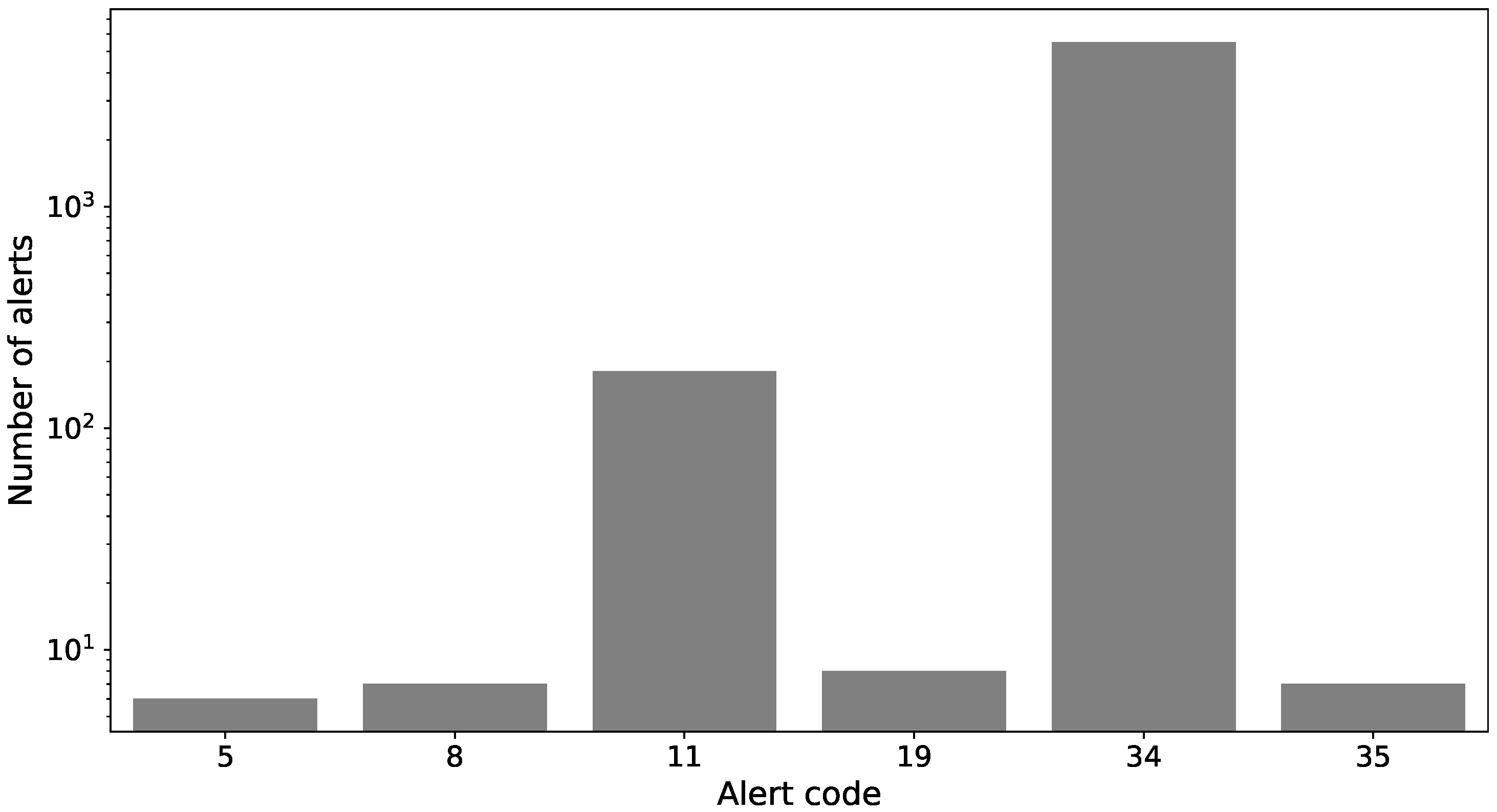
| Alert | Description |
|---|---|
| 5 | Loose carriage belt alarm |
| 8 | Film end alarm |
| 11 | Platform motor inverter protection |
| 19 | Carriage motor inverter protection |
| 34 | Machine in emergency conditions |
| 35 | Table phonic wheel sensor fault |
| Variable Name | Minimum | Maximum | Unit |
|---|---|---|---|
| Product temperature Base | −30.8 | 5.7 | °C |
| Evaporator temperature base | −37.8 | 18.2 | °C |
| Condenser temperature base | 15.8 | 36.7 | °C |
| Power supply | 134.0 | 146.0 | V |
| Instant power consumption | 0.0 | 661.0 | W |
| Signal | −113.0 | 85.0 | dBm |
| Door alert | 0 | 1 | |
| Door close | 0 | 1 | |
| Door open | 0 | 1 | |
| Machine cooling | 0 | 1 | |
| Machine defrost | 0 | 1 | |
| Machine pause | 0 | 1 |
| Name of the Alarm | Description | Number of Data Points |
|---|---|---|
| alarm 1 | High-Temperature Compartment | 2 |
| alarm 5 | High Product Temperature | 188 |
| Variable Name | Minimum | Maximum | Unit |
|---|---|---|---|
| CMS air pressure | 0.0 | 9.5 | bar |
| Oxygen base concentration | 5.0 | 500.0 | |
| Nitrogen pressure | 0.0 | 9.0 | bar |
| Oxygen over threshold | 0 | 1 |
| Name of the Alarm | Description | Number of Data Points |
|---|---|---|
| CMS pressurization fail | Pressurization of nitrogen sieve failed | 54 |
| Reading Window (RW) | Algorithm | Prediction Window (PW) | ||||||||
|---|---|---|---|---|---|---|---|---|---|---|
| 0.25 h | 0.5 h | 1.0 h | 1.5 h | 2.0 h | 2.5 h | 3.0 h | 3.5 h | 4.0 h | ||
| 10 min | ConvLSTM | 0.684 | 0.691 | 0.577 | 0.554 | 0.533 | 0.517 | 0.524 | 0.506 | 0.483 |
| LR | 0.604 | 0.598 | 0.549 | 0.518 | 0.503 | 0.498 | 0.532 | 0.514 | 0.516 | |
| LSTM | 0.758 | 0.743 | 0.634 | 0.599 | 0.583 | 0.536 | 0.550 | 0.540 | 0.512 | |
| RF | 0.577 | 0.571 | 0.429 | 0.417 | 0.402 | 0.388 | 0.382 | 0.381 | 0.391 | |
| SVM | 0.697 | 0.654 | 0.590 | 0.543 | 0.521 | 0.517 | 0.520 | 0.485 | 0.476 | |
| Transformer | 0.714 | 0.646 | 0.585 | 0.584 | 0.540 | 0.486 | 0.498 | 0.482 | 0.452 | |
| 15 min | ConvLSTM | 0.787 | 0.683 | 0.554 | 0.530 | 0.547 | 0.532 | 0.558 | 0.514 | 0.498 |
| LR | 0.742 | 0.548 | 0.516 | 0.530 | 0.513 | 0.483 | 0.526 | 0.539 | 0.540 | |
| LSTM | 0.846 | 0.753 | 0.671 | 0.590 | 0.612 | 0.593 | 0.593 | 0.547 | 0.562 | |
| RF | 0.565 | 0.391 | 0.410 | 0.363 | 0.361 | 0.376 | 0.365 | 0.349 | 0.367 | |
| SVM | 0.753 | 0.659 | 0.532 | 0.524 | 0.513 | 0.518 | 0.505 | 0.471 | 0.477 | |
| Transformer | 0.818 | 0.677 | 0.613 | 0.567 | 0.563 | 0.506 | 0.513 | 0.503 | 0.477 | |
| 20 min | ConvLSTM | 0.807 | 0.699 | 0.567 | 0.559 | 0.531 | 0.546 | 0.551 | 0.537 | 0.489 |
| LR | 0.789 | 0.696 | 0.587 | 0.554 | 0.517 | 0.518 | 0.555 | 0.585 | 0.563 | |
| LSTM | 0.861 | 0.798 | 0.665 | 0.614 | 0.559 | 0.599 | 0.611 | 0.557 | 0.557 | |
| RF | 0.538 | 0.448 | 0.404 | 0.393 | 0.381 | 0.389 | 0.379 | 0.417 | 0.384 | |
| SVM | 0.783 | 0.568 | 0.499 | 0.468 | 0.486 | 0.485 | 0.481 | 0.443 | 0.468 | |
| Transformer | 0.799 | 0.649 | 0.584 | 0.559 | 0.543 | 0.513 | 0.516 | 0.478 | 0.438 | |
| 25 min | ConvLSTM | 0.744 | 0.635 | 0.527 | 0.541 | 0.512 | 0.557 | 0.523 | 0.561 | 0.524 |
| LR | 0.735 | 0.620 | 0.552 | 0.531 | 0.519 | 0.530 | 0.580 | 0.608 | 0.575 | |
| LSTM | 0.783 | 0.686 | 0.623 | 0.612 | 0.618 | 0.577 | 0.579 | 0.568 | 0.538 | |
| RF | 0.641 | 0.433 | 0.395 | 0.379 | 0.401 | 0.433 | 0.410 | 0.401 | 0.378 | |
| SVM | 0.613 | 0.512 | 0.436 | 0.411 | 0.416 | 0.436 | 0.482 | 0.413 | 0.435 | |
| Transformer | 0.772 | 0.660 | 0.517 | 0.529 | 0.504 | 0.493 | 0.492 | 0.449 | 0.450 | |
| 30 min | ConvLSTM | 0.426 | 0.490 | 0.464 | 0.437 | 0.470 | 0.569 | 0.569 | 0.528 | |
| LR | 0.456 | 0.510 | 0.474 | 0.471 | 0.495 | 0.542 | 0.574 | 0.532 | ||
| LSTM | 0.579 | 0.588 | 0.616 | 0.612 | 0.596 | 0.598 | 0.585 | 0.553 | ||
| RF | 0.367 | 0.360 | 0.353 | 0.353 | 0.352 | 0.349 | 0.353 | 0.347 | ||
| SVM | 0.332 | 0.348 | 0.339 | 0.338 | 0.343 | 0.438 | 0.406 | 0.405 | ||
| Transformer | 0.473 | 0.505 | 0.489 | 0.474 | 0.464 | 0.443 | 0.475 | 0.443 | ||
| 35 min | ConvLSTM | 0.396 | 0.405 | 0.409 | 0.419 | 0.461 | 0.597 | 0.492 | ||
| LR | 0.410 | 0.393 | 0.393 | 0.395 | 0.473 | 0.526 | 0.492 | |||
| LSTM | 0.547 | 0.563 | 0.558 | 0.531 | 0.538 | 0.649 | 0.558 | |||
| RF | 0.333 | 0.333 | 0.333 | 0.333 | 0.332 | 0.351 | 0.343 | |||
| SVM | 0.328 | 0.328 | 0.328 | 0.329 | 0.375 | 0.428 | 0.338 | |||
| Transformer | 0.516 | 0.471 | 0.490 | 0.464 | 0.433 | 0.492 | 0.464 | |||
| Reading Window (RW) | Prediction Window (PW) | ||||||||
|---|---|---|---|---|---|---|---|---|---|
| 0.25 h | 0.5 h | 1.0 h | 1.5 h | 2.0 h | 2.5 h | 3.0 h | 3.5 h | 4.0 h | |
| 10 min | BCE | BCE | BCE | BCE | BCE | BCE | BCE | ||
| 15 min | BCE | BCE | BCE | BCE | BCE | BCE | |||
| 20 min | BCE | BCE | BCE | BCE | BCE | ||||
| 25 min | BCE | BCE | BCE | ||||||
| 30 min | |||||||||
| 35 min | |||||||||
| Reading Window (RW) | Algorithm | Prediction Window (PW) | |||
|---|---|---|---|---|---|
| 0.5 h | 1.0 h | 1.5 h | 2.0 h | ||
| 10 min | ConvLSTM | 0.750 | 0.612 | 0.634 | 0.575 |
| LR | 0.729 | 0.602 | 0.610 | 0.602 | |
| LSTM | 0.735 | 0.615 | 0.633 | 0.633 | |
| RF | 0.765 | 0.568 | 0.524 | 0.546 | |
| SVM | 0.748 | 0.635 | 0.634 | 0.612 | |
| Transformer | 0.794 | 0.621 | 0.558 | 0.659 | |
| 15 min | ConvLSTM | 0.727 | 0.615 | 0.633 | 0.615 |
| LR | 0.727 | 0.599 | 0.608 | 0.608 | |
| LSTM | 0.782 | 0.657 | 0.599 | 0.563 | |
| RF | 0.773 | 0.624 | 0.569 | 0.548 | |
| SVM | 0.742 | 0.650 | 0.640 | 0.609 | |
| Transformer | 0.787 | 0.551 | 0.556 | 0.603 | |
| 20 min | ConvLSTM | 0.680 | 0.624 | 0.617 | 0.576 |
| LR | 0.712 | 0.605 | 0.598 | 0.608 | |
| LSTM | 0.760 | 0.643 | 0.607 | 0.568 | |
| RF | 0.814 | 0.619 | 0.574 | 0.550 | |
| SVM | 0.744 | 0.648 | 0.636 | 0.614 | |
| Transformer | 0.795 | 0.633 | 0.670 | 0.659 | |
| 25 min | ConvLSTM | 0.725 | 0.634 | 0.627 | 0.542 |
| LR | 0.721 | 0.605 | 0.599 | 0.599 | |
| LSTM | 0.779 | 0.665 | 0.520 | 0.489 | |
| RF | 0.822 | 0.599 | 0.578 | 0.586 | |
| SVM | 0.738 | 0.651 | 0.634 | 0.613 | |
| Transformer | 0.758 | 0.658 | 0.607 | 0.670 | |
| 30 min | ConvLSTM | 0.730 | 0.544 | 0.601 | 0.588 |
| LR | 0.724 | 0.598 | 0.603 | 0.587 | |
| LSTM | 0.804 | 0.633 | 0.577 | 0.477 | |
| RF | 0.835 | 0.606 | 0.571 | 0.555 | |
| SVM | 0.742 | 0.635 | 0.632 | 0.606 | |
| Transformer | 0.728 | 0.646 | 0.613 | 0.519 | |
| Reading Window (RW) | Algorithm | Prediction Window (PW) | |||||
|---|---|---|---|---|---|---|---|
| 0.5 h | 1.0 h | 1.5 h | 2.0 h | 3.0 h | 5.0 h | ||
| 10 min | ConvLSTM | 0.875 | 0.900 | 0.873 | 0.879 | 0.810 | 0.792 |
| LR | 0.812 | 0.824 | 0.841 | 0.835 | 0.660 | 0.674 | |
| LSTM | 0.874 | 0.872 | 0.869 | 0.856 | 0.865 | 0.806 | |
| RF | 0.931 | 0.885 | 0.883 | 0.883 | 0.844 | 0.838 | |
| SVM | 0.903 | 0.882 | 0.885 | 0.871 | 0.807 | 0.771 | |
| Transformer | 0.874 | 0.879 | 0.871 | 0.890 | 0.828 | 0.811 | |
| 15 min | ConvLSTM | 0.830 | 0.904 | 0.798 | 0.868 | 0.830 | 0.848 |
| LR | 0.837 | 0.837 | 0.840 | 0.828 | 0.663 | 0.676 | |
| LSTM | 0.818 | 0.892 | 0.887 | 0.879 | 0.830 | 0.807 | |
| RF | 0.919 | 0.892 | 0.876 | 0.878 | 0.834 | 0.838 | |
| SVM | 0.894 | 0.879 | 0.875 | 0.874 | 0.810 | 0.784 | |
| Transformer | 0.892 | 0.888 | 0.893 | 0.883 | 0.839 | 0.821 | |
| 20 min | ConvLSTM | 0.888 | 0.893 | 0.882 | 0.876 | 0.856 | 0.812 |
| LR | 0.832 | 0.837 | 0.841 | 0.826 | 0.670 | 0.678 | |
| LSTM | 0.834 | 0.885 | 0.906 | 0.878 | 0.813 | 0.814 | |
| RF | 0.902 | 0.890 | 0.873 | 0.882 | 0.843 | 0.834 | |
| SVM | 0.882 | 0.877 | 0.873 | 0.881 | 0.815 | 0.795 | |
| Transformer | 0.896 | 0.891 | 0.896 | 0.888 | 0.813 | 0.825 | |
| 25 min | ConvLSTM | 0.842 | 0.872 | 0.887 | 0.890 | 0.809 | 0.823 |
| LR | 0.845 | 0.838 | 0.854 | 0.827 | 0.675 | 0.680 | |
| LSTM | 0.814 | 0.893 | 0.888 | 0.879 | 0.832 | 0.811 | |
| RF | 0.914 | 0.883 | 0.873 | 0.880 | 0.857 | 0.836 | |
| SVM | 0.872 | 0.882 | 0.873 | 0.887 | 0.829 | 0.803 | |
| Transformer | 0.877 | 0.861 | 0.905 | 0.898 | 0.838 | 0.836 | |
| 30 min | ConvLSTM | 0.752 | 0.881 | 0.887 | 0.882 | 0.850 | 0.796 |
| LR | 0.863 | 0.848 | 0.864 | 0.825 | 0.691 | 0.687 | |
| LSTM | 0.848 | 0.865 | 0.910 | 0.885 | 0.852 | 0.812 | |
| RF | 0.892 | 0.880 | 0.873 | 0.871 | 0.868 | 0.839 | |
| SVM | 0.863 | 0.878 | 0.879 | 0.889 | 0.837 | 0.817 | |
| Transformer | 0.868 | 0.879 | 0.912 | 0.898 | 0.821 | 0.820 | |
| Wrapping Machine | Blood Refrigerator | Nitrogen Generator | |
|---|---|---|---|
| RF | 1.40 | 0.65 | 0.04 |
| SVM | 2.10 | 0.72 | 0.15 |
| LR | 1.90 | 0.68 | 0.10 |
| LSTM | 20.00 | 4.00 | 4.80 |
| ConvLSTM | 46.00 | 1.50 | 1.93 |
| Transformer | 19.00 | 1.70 | 3.85 |
Disclaimer/Publisher’s Note: The statements, opinions and data contained in all publications are solely those of the individual author(s) and contributor(s) and not of MDPI and/or the editor(s). MDPI and/or the editor(s) disclaim responsibility for any injury to people or property resulting from any ideas, methods, instructions or products referred to in the content. |
© 2024 by the authors. Licensee MDPI, Basel, Switzerland. This article is an open access article distributed under the terms and conditions of the Creative Commons Attribution (CC BY) license (https://creativecommons.org/licenses/by/4.0/).
Share and Cite
Pinciroli Vago, N.O.; Forbicini, F.; Fraternali, P. Predicting Machine Failures from Multivariate Time Series: An Industrial Case Study. Machines 2024, 12, 357. https://doi.org/10.3390/machines12060357
Pinciroli Vago NO, Forbicini F, Fraternali P. Predicting Machine Failures from Multivariate Time Series: An Industrial Case Study. Machines. 2024; 12(6):357. https://doi.org/10.3390/machines12060357
Chicago/Turabian StylePinciroli Vago, Nicolò Oreste, Francesca Forbicini, and Piero Fraternali. 2024. "Predicting Machine Failures from Multivariate Time Series: An Industrial Case Study" Machines 12, no. 6: 357. https://doi.org/10.3390/machines12060357
APA StylePinciroli Vago, N. O., Forbicini, F., & Fraternali, P. (2024). Predicting Machine Failures from Multivariate Time Series: An Industrial Case Study. Machines, 12(6), 357. https://doi.org/10.3390/machines12060357