Erosion Analysis and Optimal Design of Sand Resistant Pipe Fittings

Abstract

Erosion of solid particles in a pipe elbow containing a 90° angle is investigated by simulation methods. In the process of shale gas exploitation, the impact of solid particles carried by fluid on the inner surface wall of pipes, as well as the turbulent flow, cause the erosion of pipes, which brings about heavy economic losses for the oil and gas industry. In the impact erosion of the inner surface wall of the pipe, the worst erosion occurs at the elbow. In this study, the erosion of a pipe elbow which has been widely used in actual production is analyzed, and the influence of the fluid velocity, the solid particle size, and the wall roughness on the erosion is investigated. Additionally, the simulation results of the erosion with the rebound and freeze boundary conditions are compared, indicating that setting the freeze boundary condition could significantly improve the computational efficiency by 74% with the acceptable accuracy. In order to reduce the impact erosion in the pipe elbow containing a 90° angle, an optimal design is proposed that can reduce the maximum erosion rate by 52.4%. These results complement the research of elbow erosion and provide ideas for the optimization problem of a pipe elbow containing a 90° angle.

1. Introduction

As an economical and efficient fluid transport system, the pipeline system is widely used in water conservancy, as well as construction, ocean, aerospace and many other fields. The erosion problem of pipes is becoming more and more serious; therefore researchers have conducted a lot of related research into mitigating the damage to a pipe by erosion [1,2,3,4]. At present, the total length of built pipelines has reached 3.5 million kilometers, and thus it is particularly critical to ensure the reliable operation and safe transportation of the pipeline system [5]. In the process of shale gas exploitation, the impact of fracturing water carrying solid particles on the inner surface wall of the pipe causes pipe erosion, which brings huge economic losses to the oil and gas industry every year. The erosion that occurs in the pipe is mainly concentrated in the elbow section, where solid particles cross the flow line and impact the elbow at high velocity [6].

With the development of CFD, researchers have proposed a variety of numerical analysis and calculation methods for pipe erosion based on different pipe models [7,8]. For example, Wang et al. investigated the unsteady slurry erosion process in the 90° elbow via the LES Eulerian–Lagrangian methodology [9]. Wang et al. investigated the slurry erosion processes of horizontal elbows numerically by the Eulerian–Lagrangian method, coupled with the particle rebound and erosion model [10]. Yang et al. carried out erosion wear experiments of fracturing pipelines under varying conditions and proposed erosion wear prediction models based on sufficient experimental data by using different machine learning algorithms [11]. Zhang et al. proposed a novel numerical procedure to analyzing solid particle erosion caused by slurry [12]. Zhang et al. developed a general numerical method to analyze solid particle erosion in a gas–liquid mixed pipeline [13]. Based on the existing energy-minimization multiscale model for turbulent flow in pipes, an improved version was proposed in which not only a new radial velocity distribution was introduced, but also the quantification of total dissipation over the cross-section of pipe was improved for the dominant mechanism of fully turbulent flow in pipe [14]. Yao et al. optimized the problem of particle penetration in the CFD–DEM method considering the influence of power-law fluid in the algorithm [15], etc.

When the erosion analysis of the pipe is finished, we need to optimize the design to reduce the wear of the pipe generated by the erosion. Wang et al. proposed an orthogonal experimental design based on the optimization method for the nozzle geometry of an underwater abrasive water jet [16]. A 90° elbow equipped with guide vanes was developed with the intent of reducing elbow erosion [17]. There are many optimization designs at the elbow [6,18,19,20] and straight sections of the pipe [21,22,23,24], including the addition of a vortex chamber in the elbow section [18], the blocking tee replacement [19], the bionic erosion resistance wall [20], and the spiral structure in the straight section of the pipe [21]. The orientation of the flow pipe [25,26] and the design of the new erosion experimental device [27,28,29] are also studied. Additionally, the detection of pipe elbow erosion levels has been combined with the percussion method and deep learning [30]. Compared with other pipeline erosion studies [31], the biggest difference in this study is that the elbow section contains the 90° angle. Although most of the current research is on ordinary elbows, elbows containing 90° angles are also widely used in engineering.

In this paper, the influence of the fluid velocity, the solid particle size, and the wall roughness on the erosion of the pipe elbow are investigated numerically. To increase the computational efficiency, the rebound and freeze boundary conditions are considered and analyzed. Compared with the results of the rebound boundary condition, it should be considered that the freeze boundary can largely shorten the computational cost with acceptable accuracy; thus, the rebound boundary condition can be replaced by the freeze one, greatly improving the development of erosion research. Compared with the previous works, an improved design of the pipe elbow wherein a quarter circular ring-cylinder is added on the inside of the elbow is proposed. The maximum erosion rate of the improved elbow can be reduced by 52.4%. Those findings provide a systematic guidance for the erosion analysis and novel designs of sand resistant pipe fittings.

2. Erosion Analysis

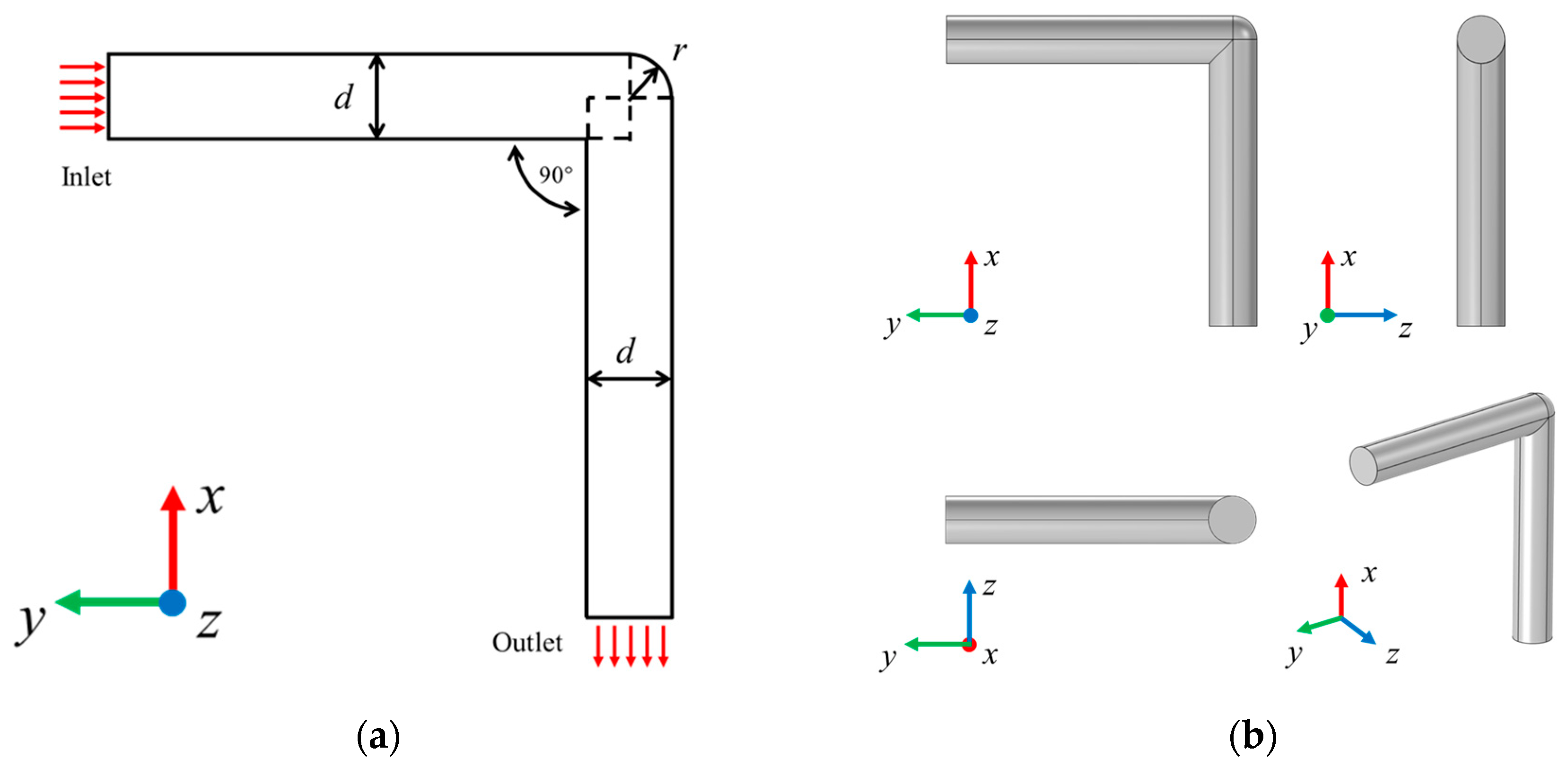
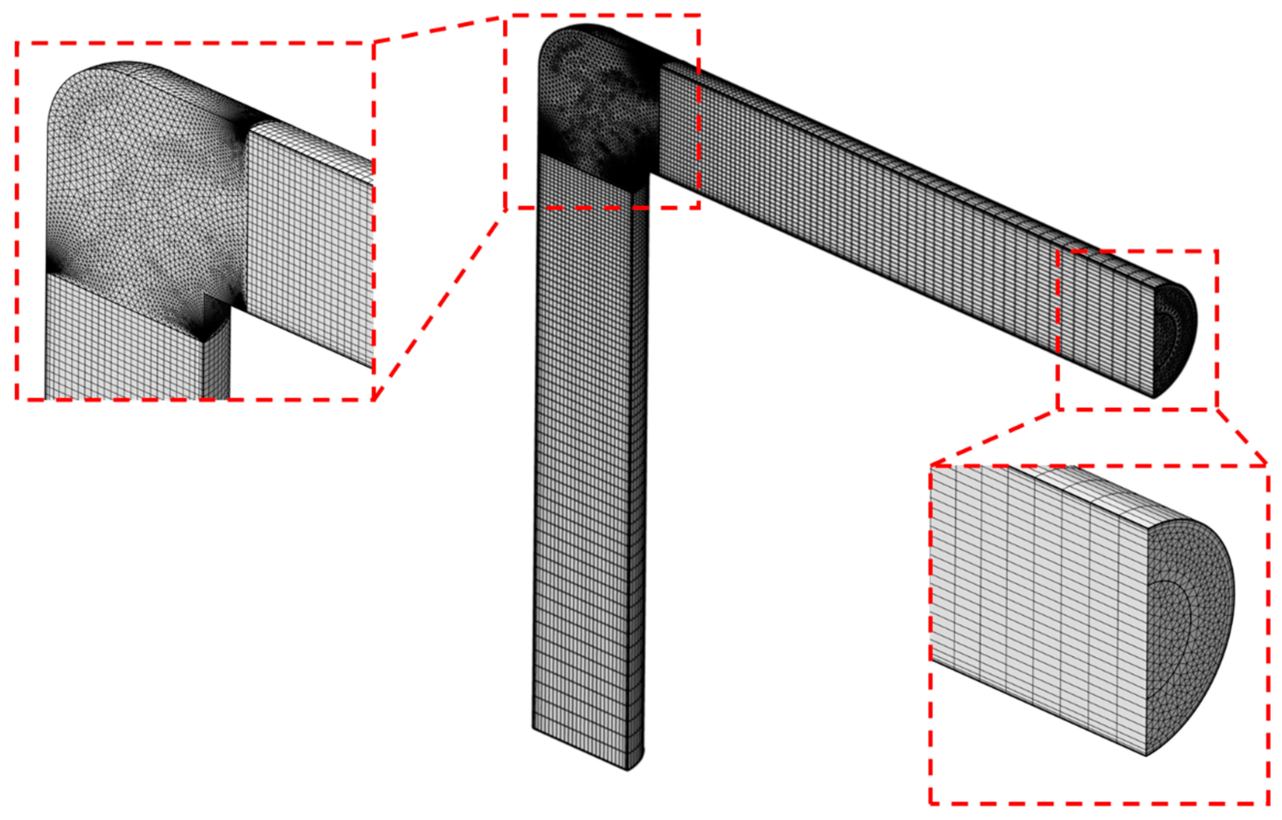
2.1. Geometric Construction

The pipe elbow in this study is shown in Figure 1, consisting of the external contour and core. A 3D model is established in Figure 2. wherein two cylinders with the same inner diameter d = 65 mm are connected by the elbow, and the angle of the inner part of the elbow core is 90°, while the outer part is an arc with a radius r equal to the cylinder radius. The four views of the 3D model are shown in Figure 2b. In this study, the commercial software COMSOL Multiphysics 6.2 is adopted for the numerical calculations involving the Turbulent Flow k-ω and Particle Tracing for Fluid Flow physics.

For fluid flow with a high Reynolds number (Re = ρVd/μ = 983 × 8 × 0.065/0.001, which is approximately equal to 5 × 10⁵ and much larger than 2300), which is the actual case in most practical engineering applications, a turbulence model with wall functions should be employed. The k-ω turbulence model is employed in fluid calculation, and thus the fluid is carried out in a steady state. Since this study focuses on the erosion of sand resistant pipe fittings in the process of oil and gas exploitation, the fluid is considered to be incompressible in computation. The fully developed flow fluid with an average speed is assumed at the inlet. The static pressure on the surface of outlet is set as 0. The fluid is fully discharged through the outlet without the generated backflow. The outside surface of the whole flow fluid model could be regarded as a wall, and the static and no-slip boundary condition should be adopted. According to the collaborative practical engineering project with the Beijing Petroleum Machinery Company (Beijing, China), the pipe is lined with ceramic materials, and the roughness is comprehensively set as 0.8, while the roughness height is set as 3.2 μm. The fluid of this study is liquid water. In this study, the discrete phase particles are conceived as spherical sand particles with a density of 2200 kg/m³, and the average diameter of the particles is set as 0.45 mm, while the mass flow rate is set as 0.1 kg/s. Fluids and solid particles are placed separately in pipe and coupled together by drag forces during the simulation. Thus, the sand mass flow rate is individually set, and it does not depend on the velocity change in the fluid. Additionally, 5000 particles are released with the fluid flow from the surface of the inlet each analysis step. The velocity of fluid flow will be stated separately before each analysis, and the movement time of solid particles in the pipe is 0.36 s. The velocity and pressure fields are solved by using linear function. In the equations for momentum, the nonlinear convective terms are discretized using a spatially second-order accurate upwind scheme. The transient solver for particles is set as GMRES. In this study, there is no coupling particle with the gas flow, as we only released solid particles in the fluid. To ensure the accuracy and efficiency, the 3D symmetric mode is adopted. The inlet and outlet boundary parts are meshed by the free triangle element, as shown in Figure 3, while five boundary layers are set near the wall for the inlet and outlet section. To describe the corrosive behavior of the elbow precisely, the mesh is divided by a gradient scanning mode. The closer the mesh is to the elbow, the denser the mesh division is.

Since the 90° vertical corner at the elbow section cannot be meshed by sweep method, free tetrahedral meshes are used to construct the pre-divided elbow area. The flow in our study is steady, thus it can be simulated in a symmetrical way. There are four different size grid schemes in

Table 1. Grid-independence.

Maximum Mesh Size (mm)	Number of Mesh	Pressure (Pa)
7	139,131	66,400
4	203,756	64,300
2.77	317,450	62,700
2.4	410,279	61,500

. The difference of the calculation results for the maximum mesh size 2.77 mm, and 2.4 mm is less than 2%. Considering the efficiency and accuracy, the scheme of 2.77 mm is adopted for calculation. In total, 317,450 grids are divided, with the size of mesh ranging from 0.181 mm to 2.77 mm, and the average quality of the mesh is 0.7 in skewness.

2.2. Numerical Model

The discrete phase model is based on the Euler–Lagrange method. In this model, the particle group is regarded as a discrete phase, described by a Lagrange coordinate system, and the fluid phase is regarded as a continuous medium, described by the Eulerian coordinate system. A discrete phase composed of particles is distributed in the continuous phase, and the corresponding mathematical method is the Euler–Lagrange method. In this model, the interaction between particle groups and the fluid medium is considered as well as the interaction between particle groups themselves. In the discrete phase model, the collision process of particles is simulated by the transfer of heat, mass and momentum between particle groups. The differential equation for particle force in the Lagrange coordinate system is solved by integrating the discrete phase particles, and the velocity field and concentration distribution of particles are obtained to determine the motion trajectory. The coupling between the continuous phase and discrete phase can be calculated by bidirectional fluid–solid coupling or unidirectional fluid–solid coupling.

In unidirectional fluid–solid coupling calculations, the transport equation under the Euler coordinate system is first solved for the continuous phase. Then, the force of the fluid on particles is coupled to the subsequent continuous phase calculation as an additional term when solving the trajectory of the discrete phase. The process of energy gain and loss in the discrete phase movement is tracked at the same time. This means that in two-phase flow calculations, the continuous phase can affect the motion of discrete phase particles; however, the discrete phase particles do not affect the flow field of the surrounding continuous phase. The influence of a discrete relative continuous phase is considered in the bidirectional fluid–solid coupling calculation, and the governing equations of fluid motion and particle motion are solved by alternating coupling until convergence. The effect of fluid on sand particles is mainly through drag force and turbulent pulsation, while the effects of sand particles on fluid are mainly to reduce the momentum and turbulent kinetic energy of fluid.

RANS k-ω turbulence model is adopted for the turbulence analysis. The continuity equations are given as

$$\nabla \cdot \left({\mathsf{\rho }}_u\overrightarrow{u}\right)\overrightarrow{u}=\nabla \cdot \left[-p\overrightarrow{I}+\overrightarrow{K}\right]+\overrightarrow{F}$$

(1)

$$\nabla \cdot \left({\mathsf{\rho }}_u\overrightarrow{u}\right)=0$$

(2)

Here, p is the pressure, u the superficial velocity of the fluid, ρ_u is the fluid density, $\overrightarrow{I}$ is the unit tensor, $\overrightarrow{F}$ is body force, and the momentum equation $\overrightarrow{K}$ can be denoted as

$$\overrightarrow{K}=\left(\mathsf{\mu }+{\mathsf{\mu }}_T\right)\left(\nabla \overrightarrow{u}+{\left(\nabla \overrightarrow{u}\right)}^T\right)$$

(3)

where μ is the kinetic viscosity, and μ_T is the turbulent kinetic viscosity.

At last, the following turbulent flow equations are used

$$\nabla \cdot \left({\mathsf{\rho }}_u\overrightarrow{u}\right)k=\nabla \cdot \left[\left(\mathsf{\mu }+{\mathsf{\rho }}_u\frac{k}{\mathsf{\omega }}{\sigma }_k\right)\nabla \cdot k\right]+{\mathsf{\rho }}_u\frac{k}{\mathsf{\omega }}\left[\nabla \overrightarrow{u}:\left(\nabla \overrightarrow{u}+{\left(\nabla \overrightarrow{u}\right)}^T\right)\right]-{\mathsf{\beta }}_0{\mathsf{\rho }}_u\mathsf{\omega }k$$

(4)

$$\nabla \cdot \left({\mathsf{\rho }}_u\overrightarrow{u}\right)\mathsf{\omega }=\nabla \cdot \left[\left(\mathsf{\mu }+{\mathsf{\rho }}_u\frac{k}{\mathsf{\omega }}{\sigma }_{\mathsf{\omega }}\right)\nabla \mathsf{\omega }\right]+\mathsf{\alpha }{\mathsf{\rho }}_u\left[\nabla \overrightarrow{u}:\left(\nabla \overrightarrow{u}+{\left(\nabla \overrightarrow{u}\right)}^T\right)\right]-{\mathsf{\rho }}_u{\mathsf{\beta }}_0{\mathsf{\omega }}^2$$

(5)

where k is the turbulent kinetic energy; ω is the dissipation rate; α is the incident angle; ${\mathsf{\sigma }}_k$, ${\mathsf{\sigma }}_{\mathsf{\omega }}$, and ${\mathsf{\beta }}_0$ are the damping functions.

The erosion process of solid particles on the pipe wall is quite complex. A large number of scholars have proposed several erosion models [32] through theoretical or experimental research. For most of the ductile materials, erosion changes with impact angle and velocity, and thus the Finnie erosion model [33,34] is used for the calculation of the erosion rate. For convenience, some assumptions are taken into account. The displaced volume is assumed to be the volume removed by the idealized particle, and the particles are rigid and do not fracture without initial rotation, while rotations of the particles are quite small during the cutting process. The Finnie erosion model is shown as

$$E_M={\displaystyle \sum _j\frac{c_i\mathsf{\rho }{m}_p{f}_{rel}{v}_j^2}{14H_V}}{\cos }^2\mathsf{\alpha },\tan \mathsf{\alpha }>\frac{P}{2},$$

(6)

$$E_M={\displaystyle \sum _j\frac{2c_i\mathsf{\rho }{m}_p{f}_{rel}{v}_j^2}{14H_{V}P}}\left[\sin \left(2\mathsf{\alpha }\right)-\frac{2}{P}{\sin }^2\mathsf{\alpha }\right],\tan \mathsf{\alpha }\le \frac{P}{2},$$

(7)

where E_M is the erosion rate, c_i is the truncated particle fraction, H_V is the surface hardness, ρ is the surface mass density, m_p is the sand mass flow rate, f_rel is the release frequency of particles, v_j is the relative velocity of sand, the erosion model is established by considering the low and high incidence angles. Here,

$$P=K/\left(1+m_P{r}_P^2/I_P\right)$$

(8)

where I_P is the particle moment of inertia, K is the ratio of normal and tangential forces, r_P is the radius of the particle. Thus, the erosion rates can be obtained by solving the above equations. Some parameters for erosion calculation are shown in

Table 2. Parameters of erosion simulation model.

Truncated Particle Fraction ci	Normal and Tangential Force Ratio K	Surface Hardness HV (GPa)	Surface Mass Density ρ (kg/m3)	Particle Radius rP (mm)	Sand Mass Flow Rate mp (kg/s)
0.1	2	1.2	3900	0.225	0.1

.

Since a sand particle will repeatedly collide with the pipe wall, the energy transfer and loss generated by the wall during the collision make the rebound velocity smaller than the impact collision velocity, it is necessary to establish a collision-rebound model between the sand particle and the wall. The energy loss of solid sand particles is usually measured by the ratio of the velocity components before and after collision, and the recovery coefficient is used to describe this effect. Stochastic recovery coefficients proposed by Grant and Tabakoff [35] are used in the erosion simulation in this study, and the normal and tangential recovery coefficients can be calculated as

$${\mathsf{\epsilon }}_N=0.993-1.76\mathsf{\alpha }+1.56{\mathsf{\alpha }}^2-0.49{\mathsf{\alpha }}^3$$

(9)

$${\mathsf{\epsilon }}_T=0.988-1.66\mathsf{\alpha }+2.11{\mathsf{\alpha }}^2-0.67{\mathsf{\alpha }}^3$$

(10)

The numerical model should be validated before further analysis. Considering that the study with a high Reynolds number is more consistent with engineering practice and our numerical model, the erosion results of pipe bends considering fluid-induced stress [4,36] are adopted here to be reproduced by the Turbulent Flow k-ω and Particle Tracing for Fluid Flow physics in this work. The comparison of the erosion results is shown in Figure 4, and our numerical results have a good agreement with those in Ref. [4], which indicates that the numerical model is considered to be reasonable and feasible for simulation.

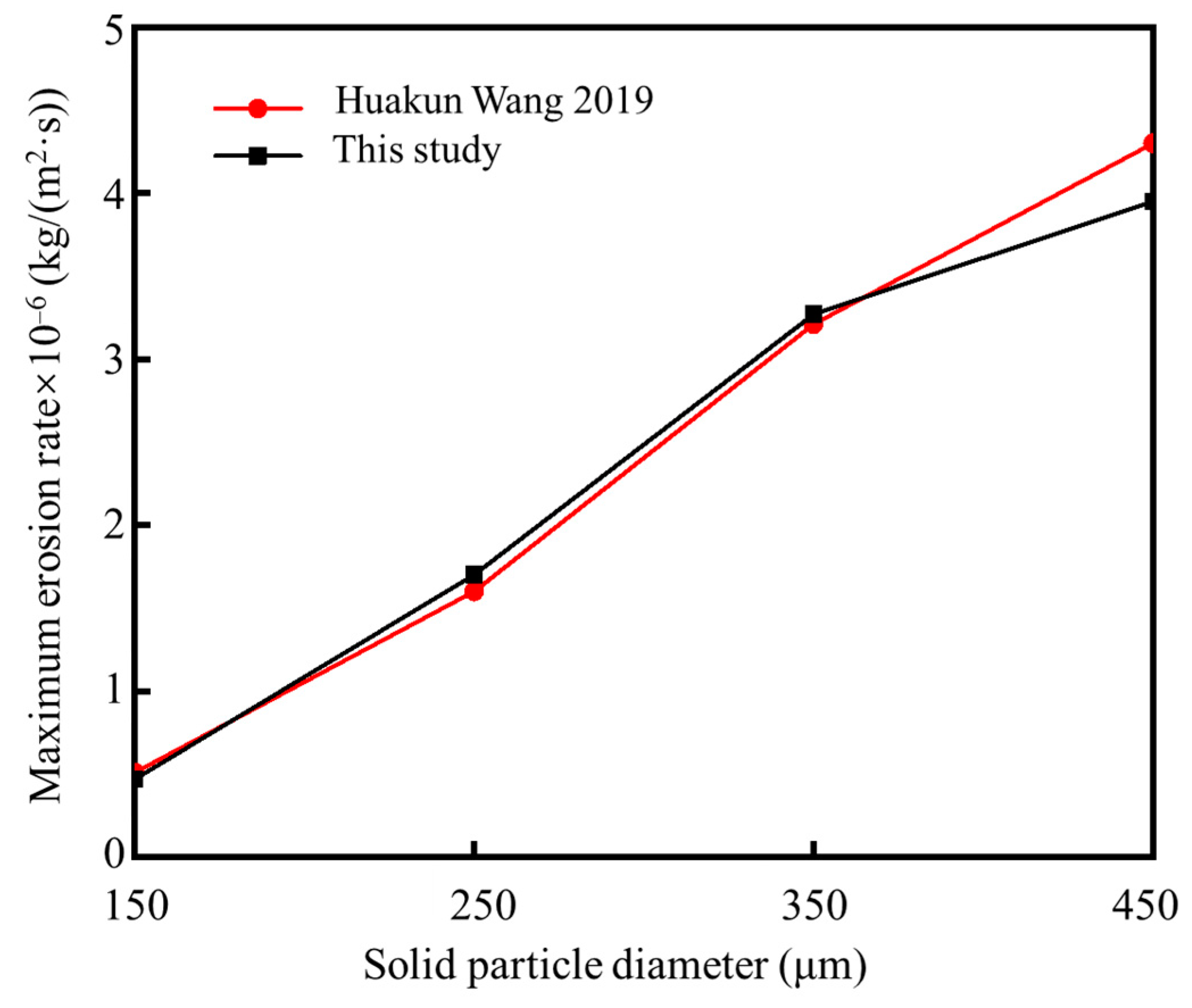
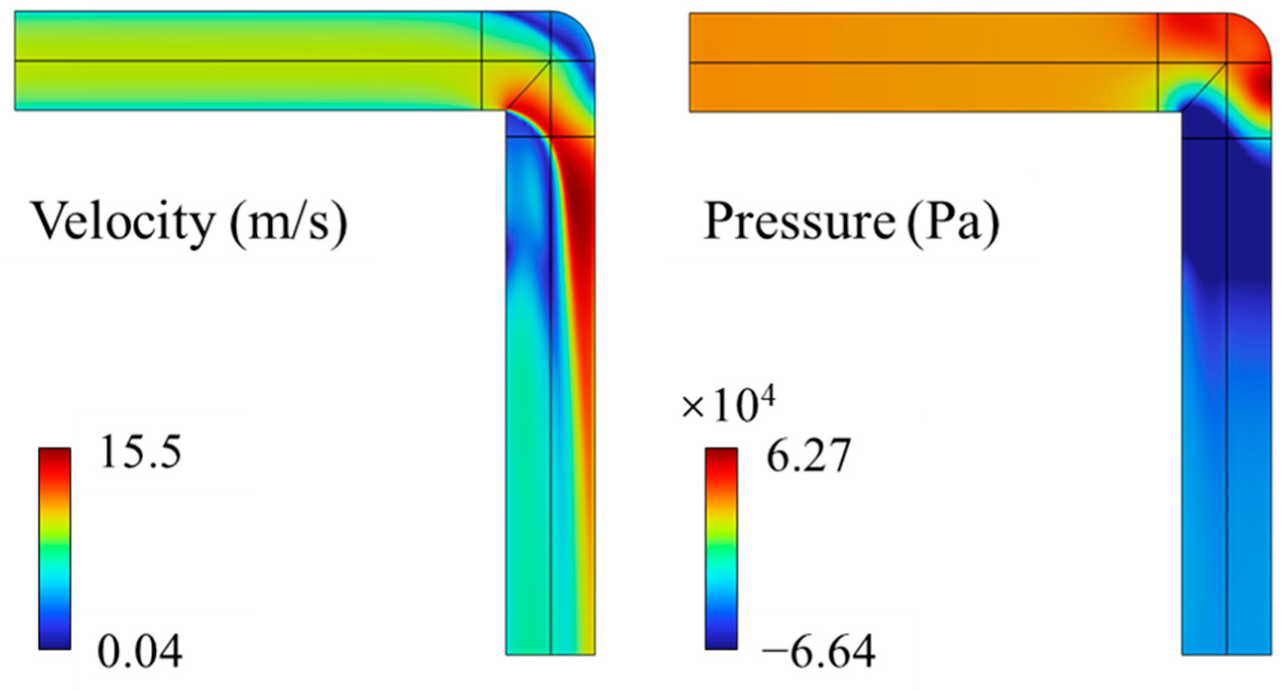
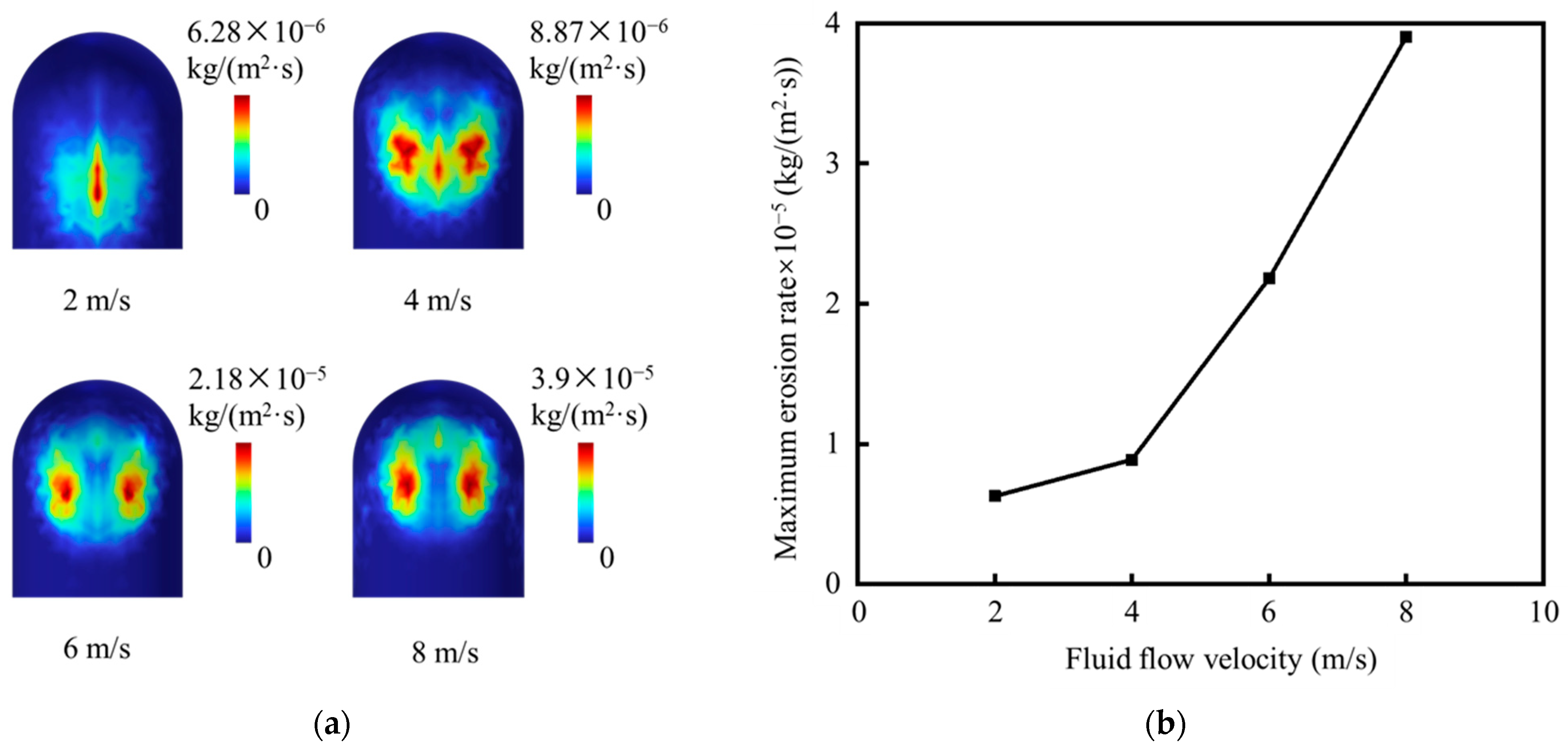
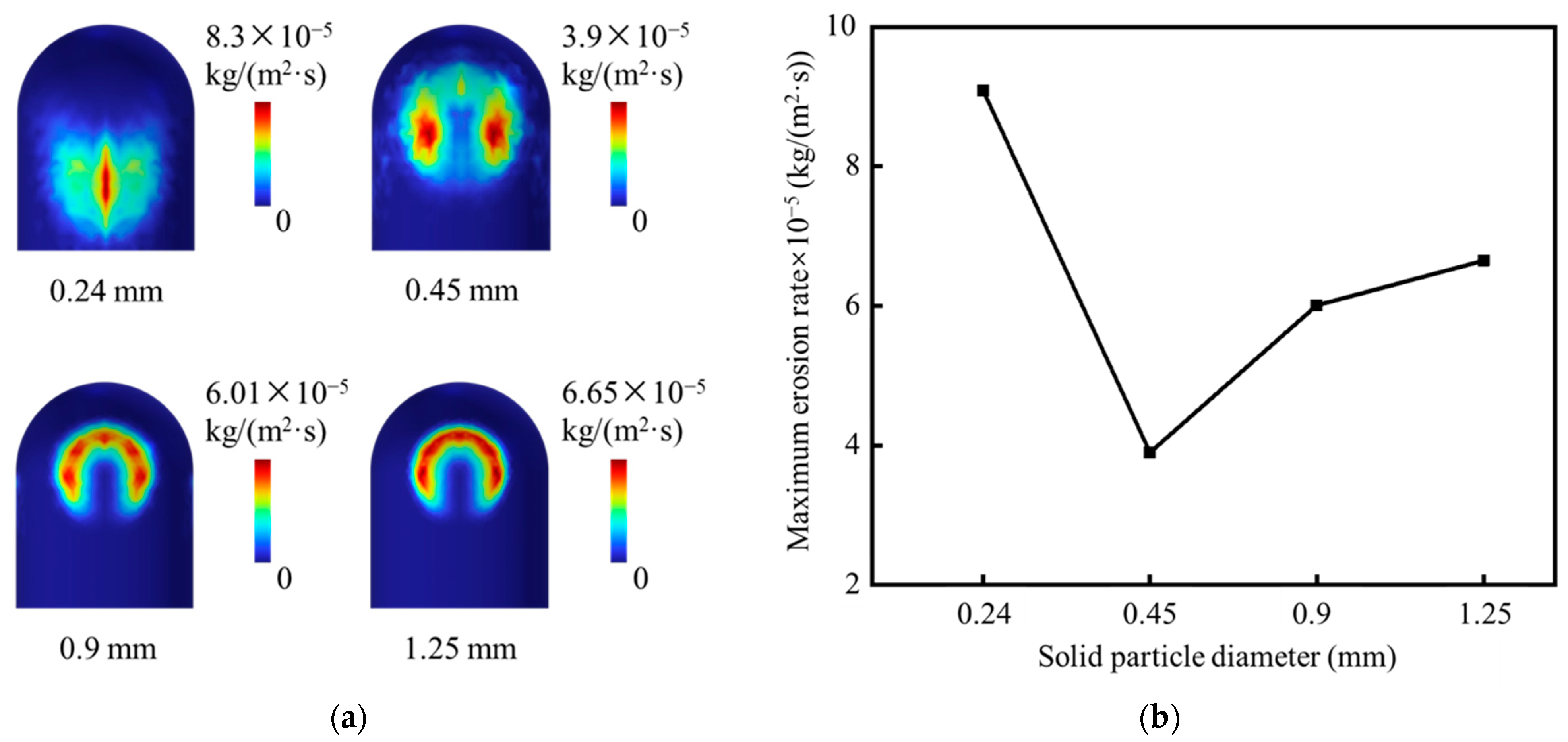
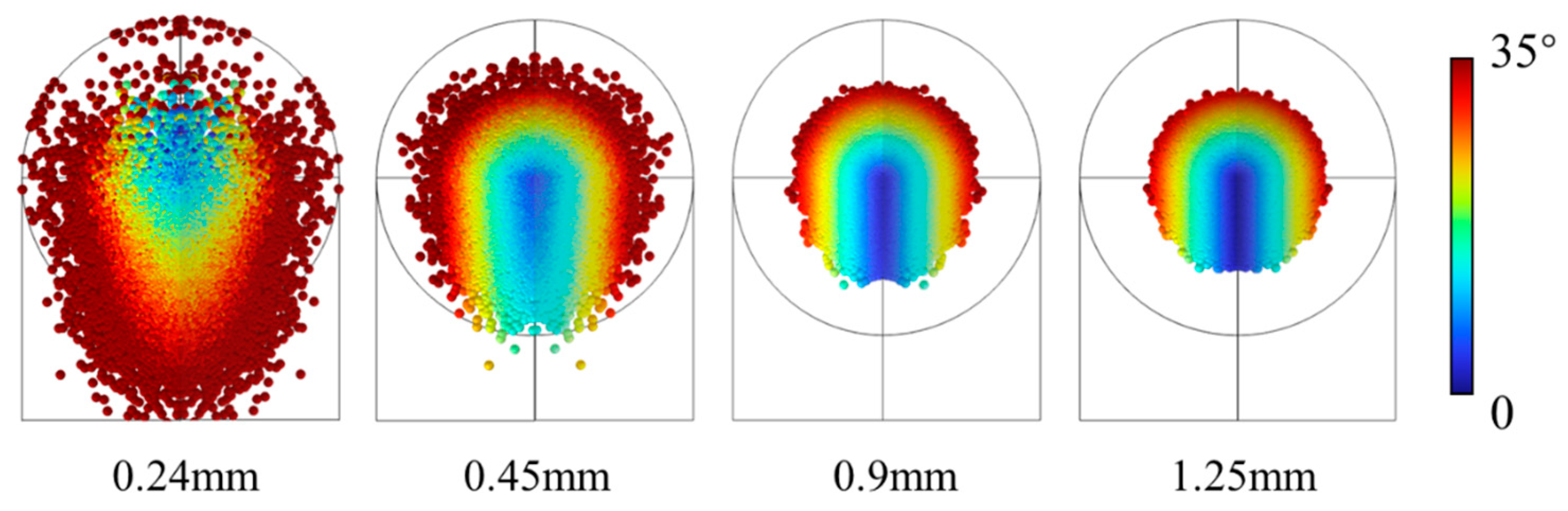
2.3. Results and Analysis

During shale gas extraction, the solid particles enter the pipe only when the valve is switched, which is not a long-term situation, and therefore, the risk in pipe security to hold the pressure is not considered in this study. The distributions of velocity and pressure at the symmetrical section of the pipeline are shown in Figure 5. It can be seen that the flow velocity of the fluid in the pipe gradually decreases from the wall to the center and from the inlet to the outlet. At the junction between the elbow and the outlet section, the inner flow velocity decreases rapidly, while the outer flow velocity increases rapidly, and the fluid flow velocity at the end of the outlet section becomes stable. In the pipe, the fluid flow begins to turn at the elbow, and a small vortex chamber is formed in the upper right corner of the elbow section. Due to the 90° corner, the fluid is collected when it comes through the elbow section, forming a high-speed zone. The velocity of the fluid in the inner part of the outlet section decreases because only a small fraction of the fluid passes through here.

It can be seen that the pressure in the pipe generally maintains a large pressure in the inlet section. The pressure inside the pipe increases to the maximum on the outside of the elbow and decreases to the minimum on the inside of the elbow. The fluid pressure in the pipe forms a negative pressure zone at the junction of the elbow and the outlet section. Based on the analysis of distributions of velocity and pressure, it is concluded that the maximum velocity and the maximum pressure in the pipe are both outside of the elbow. Since the maximum erosion of solid particles on the pipe wall should be in the same location, improving the elbow section is a feasible scheme to reduce the erosion of the pipeline. The influence factors of fluid and solid particles on pipe erosion vary, and so erosion analysis of three influence parameters is carried out, based on a fluid flow velocity of 8 m/s, a solid particle diameter of 0.45 mm, and a wall roughness of 0.8, which are derived from the practical engineering. Unless otherwise stated, three influence parameters are fixed as above in the following results.

For four different fluid flow velocities, the erosion rates of fluid and solid particles on the pipe wall are shown in Figure 6a, where the positions of the erosions on the pipe wall are colored. It is obvious in Figure 6 that the maximum erosion rate increases with the increase in fluid flow velocities. The analysis shows that when the fluid flow velocity is less than 4 m/s, some solid particles begin to collide with the pipe wall before entering the elbow section. In other words, due to the low velocity, some solid particles are removed from the influence of the fluid drag force in the inlet section, and thus part of solid particles do not enter elbow section. However, when the fluid flow velocity is over 4 m/s, all the solid particles are driven by the fluid drag force into the elbow section to produce erosion. At this time, the erosion rate depends on the fluid flow velocity.

Furthermore, the maximum erosive position and the entire erosive region move upward with the increase in fluid flow velocity shown in Figure 6a. Since the velocity of the solid particles is provided by the drag force of the fluid, the velocity and direction of the solid particles motion in the fluid are hysteresis relative to the fluid. At the elbow, the flow direction of the fluid changes by the 90° corner immediately, but the solid particles still move with the initial direction. At the same time, the movement direction of the solid particles also changes with the fluid flow. This change becomes more difficult when the movement velocity of the solid particles is higher. As a result, the position of erosion is constantly moving up.

For different solid particle diameters, the erosion rates of fluid and solid particles on the pipe wall are shown in Figure 7, where the positions of erosions on the pipe wall are colored. The maximum erosion rates are the largest and least when the diameters of the solid particles are 0.24 mm and 0.45 mm, respectively. The maximum erosion rate increases when the solid particles diameter is over 0.45 mm. The reason is that the erosion of solid particles on the pipe wall is mainly caused by the cutting force, the tangential force of the solid particles hitting the wall. When the diameter of the solid particles is 0.24 mm, the solid particles are affected by the drag force of the fluid and converge to the maximum erosion position. At the same time, solid particles follow the changing fluid flow direction in the elbow section rapidly, which produces a large cutting force on the pipe wall at a large acute incidence angle. A large number of solid particles are continuously cut here, showing a large erosion rate. With the increase in particle sizes, the acute incidence angle of solid particles at the elbow decreases continuously due to its inertia, and the fluid is no longer able to gather the solid particles well, and thus the erosion position is dispersed on both sides of the pipe wall, as well as the cutting force received at the same position. Therefore, the maximum erosion rate decreases with the increase in particle diameter when over 0.45 mm.

To figure out this phenomenon, the incidence angles and impact locations where the solid particles impact the elbow are shown in Figure 8. The incidence angles vary continuously from 0 to 35° outwards from the central position in Figure 8. The cutting force of the particle on the pipe also increases with the increase in the incidence angle. The research indicates that the large incidence angle areas have a good agreement with the maximum erosion rates.

For different wall roughness conditions, the erosion rates of fluid and solid particles on the pipe wall are shown in Figure 9a, where the positions of erosions on the pipe wall are colored. Both the erosion positions and erosion rates have no significantly change with the various wall roughness; therefore, the wall roughness has little influence on erosions.

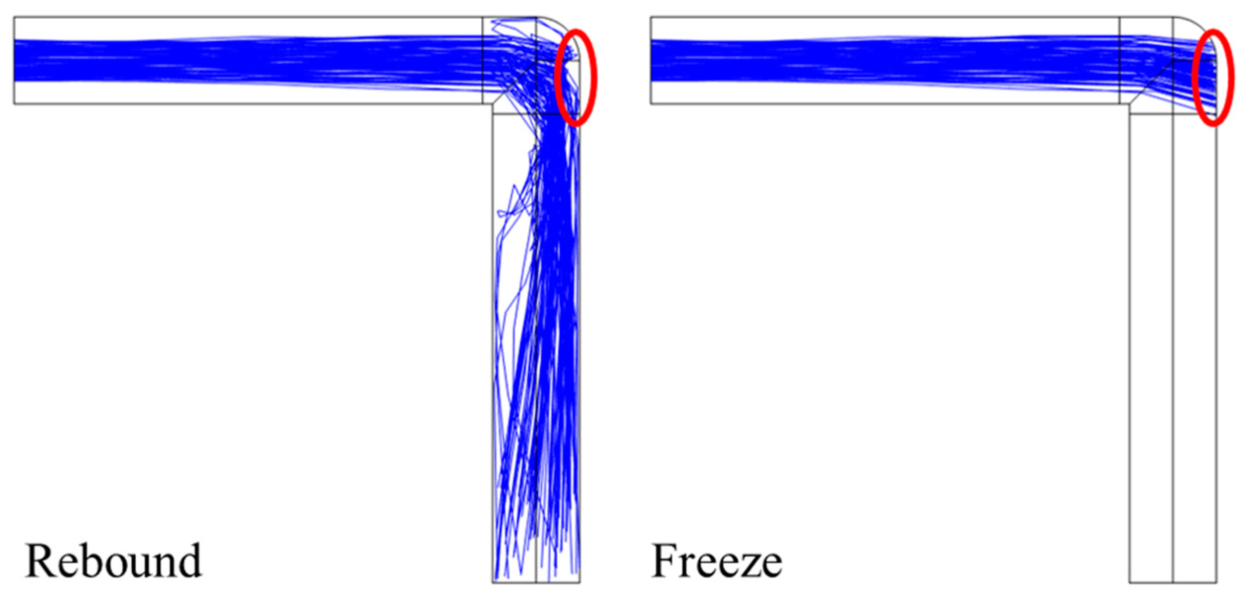
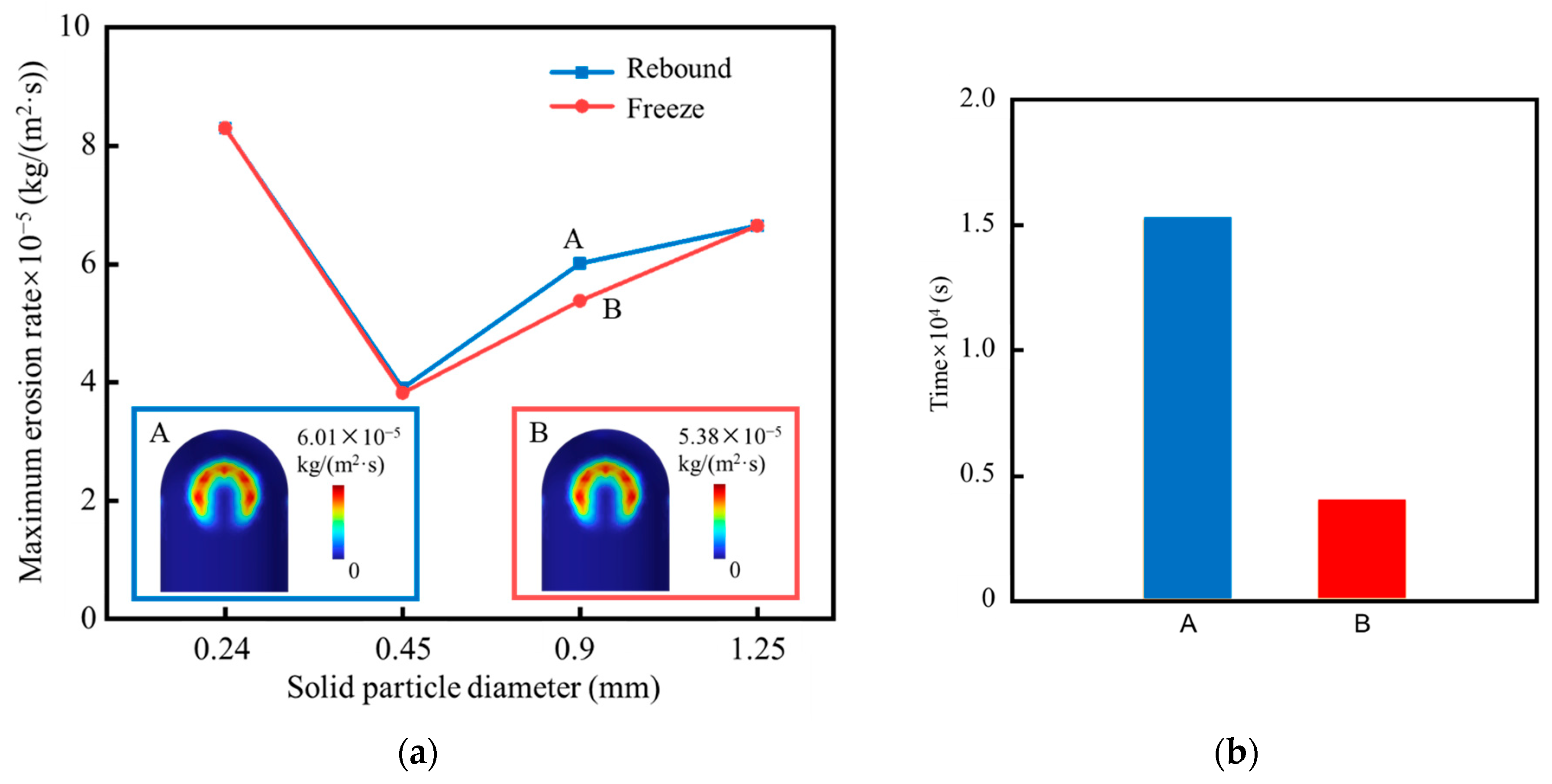
3. Comparation of Rebound and Freeze Boundary Conditions

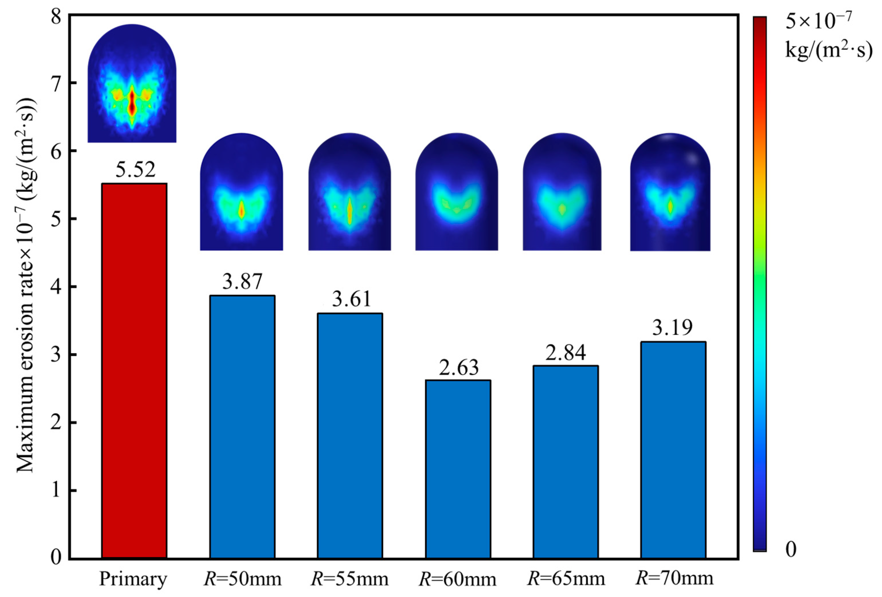
Computational efficiency is crucial in erosion analysis. In this section, the freeze boundary condition is introduced to improve the computational efficiency. Generally, the rebound boundary condition considers that solid particles collide with the wall repeatedly in the pipeline, and there should be energy loss with each collision. In the whole process of erosion, solid particles in the pipe impact the wall after several collisions, and thus the rebound boundary condition is adopted in most erosion studies. Nevertheless, when the boundary condition is considered as freeze, the positions of solid particles do not change after hitting the wall of the pipe. When the distribution of instantaneous energy and velocity between charged particles and the wall need to be analyzed, the freeze boundary condition will be adopted. Here, we take the analysis of different solid particle diameters as an example to compare rebound and freeze. Figure 10 presents the comparison of the particle trajectory considering the rebound and freeze boundary conditions. It can be seen that the positions of particles contacting the pipe are consistent when two boundary conditions are considered, marked by the red ellipses in Figure 10, which are the positions of maximum erosion. Therefore, considering that the maximum erosion rate of solid particles on pipe walls mainly occurs at the first collision in this work, it is suggested that the freeze boundary condition can be adopted instead of the rebound one.

The erosion results considering the rebound and freeze boundary conditions are shown in Figure 11. There is no significant difference between the two erosion results that both of the erosion location and maximum erosion rate are almost unchanged, which indicates that the variation trend of the maximum erosion rate is basically the same. Only for the particle diameter being 0.9 mm, the deviation is maximum as shown in Figure 11a, whereas this deviation of the erosion rate for the rebound and freeze boundary conditions is insignificant and acceptable. More importantly, compared with the rebound boundary condition, the computational cost considering the freeze boundary condition can be reduced 74% shown in Figure 11b. In a word, the rebound boundary condition can be replaced by the freeze one with much higher efficiency and acceptable accuracy.

4. Optimal Design

At present, there is little research on the elbow containing the 90° angle, which does exist in the practical engineering. Other researchers’ optimized designs for elbows can reduce erosion well, such as adding vortex chamber [13], using plugged tee [14], using spiral pipe [16], etc. This optimal design for elbows with the 90° angle is simpler and more effective. Based on the above erosion analysis, the improved pipe wall design scheme is shown in Figure 12. Here, a transition is introduced at the 90° bending position of the right-angled pipe. The transition part is a quarter circular ring cylinder, and the cross section of transition part is circular, which should overlap with the inlet of the pipe. The radius R of the center line of the circular ring cylinder is set as the optimal tunable parameter shown in Figure 12. The solid black line in Figure 12a is the complete outline of the pipe.

This design actually extends the space at the turning point, reducing the speed of the sand-bearing fluid, then decreases the collision speed between the solid particles and the pipe wall. Furthermore, the right angle of the original structure is eliminated by chamfering, which significantly reduces the incidence angle of solid particles in the collision area on the tube wall.

To verify that the optimal design is more resistant to erosion than the initial one, numerical simulations are carried out with the parameters used in general engineering practice, as listed in

Table 3. Parameters of optimal design pipe models.

Truncated Particle Fraction ci	Normal and Tangential Force Ratio K	Surface Hardness HV (GPa)	Surface Mass Density ρ (kg/m3)	Grain Density ρP (kg/m3)	Fluid Velocity u (m/s)
0.1	2	1.96	7860	2850	16.5

[37].

The initial and optimal design pipe models with various radius are simulated and analyzed, as shown in Figure 13. In comparison of the maximum erosion rates for different optimal design pipe models, it can be seen that the optimal design scheme can effectively reduce the maximum erosion rate, among which the maximum erosion rate can be reduced when the ring radius is 60 mm, and the erosion rate can be reduced by 52.4%. The relevant experimental verification will be continuously improved in the further study.

5. Conclusions

Erosion analysis and optimization design of sand resistant pipe fittings are carried out. The influence of the fluid velocity, the solid particle size and the wall roughness on the erosion are investigated. The rebound and freeze boundary conditions are analyzed and compared to increase the computational efficiency. The optimal design that can reduce the maximum erosion rate is proposed. From this study, the following conclusions can be drawn:

(1) The pipe maximum erosion appears in the transition position of the elbow and outlet section. With the increase in the fluid flow velocity in the pipe, the maximum erosion rate increases. The erosion distribution on the pipe wall mainly depends on the incidence acute angle when the solid particles collide with the pipe wall. The wall roughness of the pipe almost has no effects on the erosion.

(2) In the pipe erosion simulation, the rebound boundary condition is replaced by the freeze one to calculate the maximum erosion rate. Considering the freeze boundary condition can reduce the computational cost by 70% with enough accuracy.

(3) For the sand resistance pipe, the optimal design of the quarter circular ring cylinder is proposed, which can effectively reduce the erosion in the pipe. The maximum erosion rate in particular can be reduced by 52.4% when the ring radius is 60 mm.

The present studies and results have potential engineering applications for the erosion sand resistant pipe fittings, such as the erosion problem of a pipeline by sand-carrying drainage during shale gas exploitation.

References

1. Fetzer, R.; Weisenburger, A.; Mueller, G. Turbulent flow of liquid lead alloy in oxygen-controlled corrosion erosion test facility. AIP Adv. 2021, 11, 075303. [Google Scholar] [CrossRef]
2. Ma, S.; Li, X.; Wang, H.; Ma, J.; Du, M.; Li, F.; Ren, J. Experimental and simulation study on anti-erosion properties of ductile materials. AIP Adv. 2022, 12, 025224. [Google Scholar] [CrossRef]
3. Zhou, W.; Yin, Y.; Sun, Z.; Ma, P.; Shi, X. Numerical simulation of particle erosion in the internal flow field of solid rocket motor nozzle using Rocstar. AIP Adv. 2022, 12, 025224. [Google Scholar] [CrossRef]
4. Wang, H.; Yu, Y.; Yu, J.; Xu, W.; Li, X.; Yu, S. Numerical simulation of the erosion of pipe bends considering fluid-induced stress and surface scar evolution. Wear 2019, 440–441, 203043. [Google Scholar] [CrossRef]
5. Wu, T.; Chen, Y.; Deng, Z.; Shen, L.; Xie, Z.; Liu, Y.; Zhu, S.; Liu, C.; Li, Y. Oil pipeline leakage monitoring developments in China. J. Pipeline Sci. Eng. 2023, 3, 100129. [Google Scholar] [CrossRef]
6. Edwards, J.K.; McLaury, B.S.; Shirazi, S.A. Modeling Solid Particle Erosion in Elbows and Plugged Tees. J. Energy Resour. Technol. 2001, 123, 277–284. [Google Scholar] [CrossRef]
7. Yu, H.; Liu, H.; Zhang, S.; Zhang, J.; Han, Z. Research progress on coping strategies for the fluid-solid erosion wear of pipelines. Powder Technol. 2023, 422, 118457. [Google Scholar] [CrossRef]
8. Li, S.; Zhang, B.; Yang, L.; Zhang, J.; Wang, Y.; Kang, W. Study on Wear Properties of the Graphite-Sealing Surfaces in a Triple Eccentric Butterfly Valve Based on EDEM-Fluent Coupling. Machines 2023, 11, 463. [Google Scholar] [CrossRef]
9. Wang, Q.; Ba, X.; Huang, Q.; Wang, N.; Wen, Y.; Zhang, Z.; Sun, X.; Yang, L.; Zhang, J. Modeling erosion process in elbows of petroleum pipelines using large eddy simulation. J. Petrol. Sci. Eng. 2022, 211, 110216. [Google Scholar] [CrossRef]
10. Wang, Y.; Wang, X.; Shang, P.; Xu, Z.; Huang, Q. A numerical study of the slurry erosion in 90° horizontal elbows. J. Pipeline Sci. Eng. 2023, 100149, in press. [Google Scholar] [CrossRef]
11. Yang, S.; Zhang, L.; Fan, J.; Sun, B. Experimental study on erosion behavior of fracturing pipeline involving tensile stress and erosion prediction using random forest regression. J. Nat. Gas Sci. Eng. 2021, 87, 103760. [Google Scholar] [CrossRef]
12. Zhang, R.; Sun, L.; Li, Y.; Yin, J. Numerical analysis of solid particle erosion caused by slurry in dredging pipelines based on a particle separation method. Powder Technol. 2023, 428, 118826. [Google Scholar] [CrossRef]
13. Zhang, R.; Xu, K.; Liu, Y.; Liu, H. A general numerical method for solid particle erosion in gas–liquid two-phase flow pipelines. Ocean Eng. 2023, 267, 113305. [Google Scholar] [CrossRef]
14. Zhang, L.; Huang, W.L.; Chen, J. An improved EMMS model for turbulent flow in pipe and its solution. Particuology 2023, 76, 1–12. [Google Scholar] [CrossRef]
15. Yao, L.; Liu, Y.; Xiao, Z.; Chen, Y. An algorithm combining sedimentation experiments for pipe erosion investigation. Energy 2023, 270, 126891. [Google Scholar] [CrossRef]
16. Wang, X.; Wu, Y.; Jia, P.; Liu, H.; Yun, F.; Li, Z.; Wang, L. Orthogonal Experimental Design Based Nozzle Geometry Optimization for the Underwater Abrasive Water Jet. Machines 2022, 10, 1243. [Google Scholar] [CrossRef]
17. Li, A.; Wang, Z.; Zhu, L.; Wang, Z.; Shi, J.; Yang, W. Design optimization of guide vane for mitigating elbow erosion using computational fluid dynamics and response surface methodology. Particuology 2022, 63, 83–94. [Google Scholar] [CrossRef]
18. Duarte, C.A.R.; de Souza, F.J.; dos Santos, V.F. Mitigating elbow erosion with a vortex chamber. Powder Technol. 2016, 288, 6–25. [Google Scholar] [CrossRef]
19. Farokhipour, A.; Mansoori, Z.; Rasteh, A.; Rasoulian, M.A.; Saffar-Avval, M.; Ahmadi, G. Study of erosion prediction of turbulent gas-solid flow in plugged tees via CFD-DEM. Powder Technol. 2019, 352, 136–150. [Google Scholar] [CrossRef]
20. Yu, H.; Shao, L.; Zhang, S.; Zhang, J.; Han, Z. A new erosive wear resistance strategy for curved surfaces based on combined bionics. Tribol. Int. 2023, 180, 108226. [Google Scholar] [CrossRef]
21. Duarte, C.A.R.; de Souza, F.J. Innovative pipe wall design to mitigate elbow erosion: A CFD analysis. Wear 2017, 380–381, 176–190. [Google Scholar] [CrossRef]
22. Kannojiya, V.; Kumar, S. Assessment of Optimum Slurry Pipe Design for Minimum Erosion. Sci. Iran. 2019, 27, 2409–2418. [Google Scholar] [CrossRef]
23. Liu, E.-B.; Huang, S.; Tian, D.-C.; Shi, L.-M.; Peng, S.-B.; Zheng, H. Experimental and numerical simulation study on the erosion behavior of the elbow of gathering pipeline in shale gas field. Pet. Sci. 2023, in press. [Google Scholar] [CrossRef]
24. Zolfagharnasab, M.H.; Salimi, M.; Zolfagharnasab, H.; Alimoradi, H.; Shams, M.; Aghanajafi, C. A novel numerical investigation of erosion wear over various 90-degree elbow duct sections. Powder Technol. 2021, 380, 1–17. [Google Scholar] [CrossRef]
25. Khan, R.; Mourad, A.H.I.; Seikh, A.H.; Petru, J.; H.Ya, H. Erosion impact on mild steel elbow pipeline for different orientations under liquid-gas-sand annular flow. Eng. Fail. Anal. 2023, 153, 107565. [Google Scholar] [CrossRef]
26. Wang, S.; Shi, J.; Han, X.; Zhu, L.; Bi, J.; Wang, J.; Wang, S.; Ma, Z.; Wang, Z. Effect of pipe orientation on erosion of π-shaped pipelines. Powder Technol. 2022, 408, 117769. [Google Scholar] [CrossRef]
27. Karthik, S.; Amarendra, H.J.; Rokhade, K.K.; Prathap, M.S. Experimental and numerical approach to predict slurry erosion in jet erosion test rig. Int. J. Refract. Met. Hard Mater. 2022, 105, 105807. [Google Scholar] [CrossRef]
28. Jia, W.; Zhang, Y.; Li, C.; Luo, P.; Song, X.; Wang, Y.; Hu, X. Experimental and numerical simulation of erosion-corrosion of 90° steel elbow in shale gas pipeline. J. Nat. Gas Sci. Eng. 2021, 89, 103871. [Google Scholar] [CrossRef]
29. Xu, L.; Wu, F.; Ren, H.; Zhou, W.; Yan, Y. Experimental and numerical investigation on erosion of circular and elliptical immersed tubes in fluidized bed. Powder Technol. 2022, 409, 117820. [Google Scholar] [CrossRef]
30. Chen, J.; Cao, L.; Song, G. Detection of the pipeline elbow erosion by percussion and deep learning. Mech. Syst. Sig. Process. 2023, 200, 110546. [Google Scholar] [CrossRef]
31. Hong, B.; Li, Y.; Li, Y.; Gong, J.; Yu, Y.; Huang, A.; Li, X. Numerical simulation of solid particle erosion in the gas-liquid flow of key pipe fittings in shale gas fields. Case Stud. Therm. Eng. 2023, 42, 102742. [Google Scholar] [CrossRef]
32. Parsi, M.; Najmi, K.; Najafifard, F.; Hassani, S.; McLaury, B.S.; Shirazi, S.A. A comprehensive review of solid particle erosion modeling for oil and gas wells and pipelines applications. J. Nat. Gas Sci. Eng. 2014, 21, 850–873. [Google Scholar] [CrossRef]
33. Finnie, I. Some observations on the erosion of ductile metals. Wear 1972, 19, 81–90. [Google Scholar] [CrossRef]
34. Finnie, I. Erosion of surfaces by solid particles. Wear 1960, 3, 87–103. [Google Scholar] [CrossRef]
35. Grant, G.; Tabakoff, W. Erosion Prediction in Turbomachinery Resulting from Environmental Solid Particles. J. Aircr. 1975, 12, 471–478. [Google Scholar] [CrossRef]
36. Zeng, L.; Zhang, G.A.; Guo, X.P. Erosion–corrosion at different locations of X65 carbon steel elbow. Corros. Sci. 2014, 85, 318–330. [Google Scholar] [CrossRef]
37. Homicz, G.F. Computational Fluid Dynamics simulations of pipe elbow flow. SAND2004-3467. 2004; pp. 3–28. Available online: https://www.osti.gov/servlets/purl/919140 (accessed on 1 August 2004).
Figure 1. The illustration of pipe elbow consisting of the external contour and core.
Machines 12 00177 g001
Figure 2. (a) 2D schematic diagram of the fluid flow in the pipe; (b) Front, left, top and isometric views of 3D model.
Machines 12 00177 g002
Figure 3. Mesh division of the inlet, elbow, and outlet sections.
Machines 12 00177 g003
Figure 4. Comparison of the erosion results of pipe bends considering fluid-induced stress [4] with RANS k-ω turbulence model.
Machines 12 00177 g004
Figure 5. Distributions of velocity and pressure of the symmetrical section of the pipe.
Machines 12 00177 g005
Figure 6. (a) Erosion rates of the pipeline for different fluid flow velocities. (b) Maximum erosion rates of the pipe wall varying with the fluid flow velocities.
Machines 12 00177 g006
Figure 7. (a) Erosion rates of the pipe for different solid particle diameters; (b) Maximum erosion rates of the pipe wall varying with the solid particle diameters.
Machines 12 00177 g007
Figure 8. Distributions of incident angles that the solid particles impact the elbow.
Machines 12 00177 g008
Figure 9. (a) Erosion rate of the pipe for different wall roughness; (b) Maximum erosion rates of pipe wall varying with wall roughness.
Machines 12 00177 g009
Figure 10. Comparison of the particle trajectory considering the rebound and freeze boundary conditions.
Machines 12 00177 g010
Figure 11. (a) Comparison of maximum erosion rates under two boundary conditions; (b) Computational cost under two boundary conditions.
Machines 12 00177 g011
Figure 12. (a) Schematic diagram of optimal quarter circular ring cylinder, the radius of the center line of the circular ring cylinder is denoted as R; (b) Front, left, top, and isometric views of 3D optimal model.
Machines 12 00177 g012
Figure 13. Comparison of maximum erosion rates for different optimal design pipe models with the initial design.
Machines 12 00177 g013