
Field-Weakening Strategy with Modulated Predictive Current Control Applied to Six-Phase Induction Machines

 ,
,  ,
,  ,
,  ,
,  ,
,  , and
, and
Abstract
1. Introduction
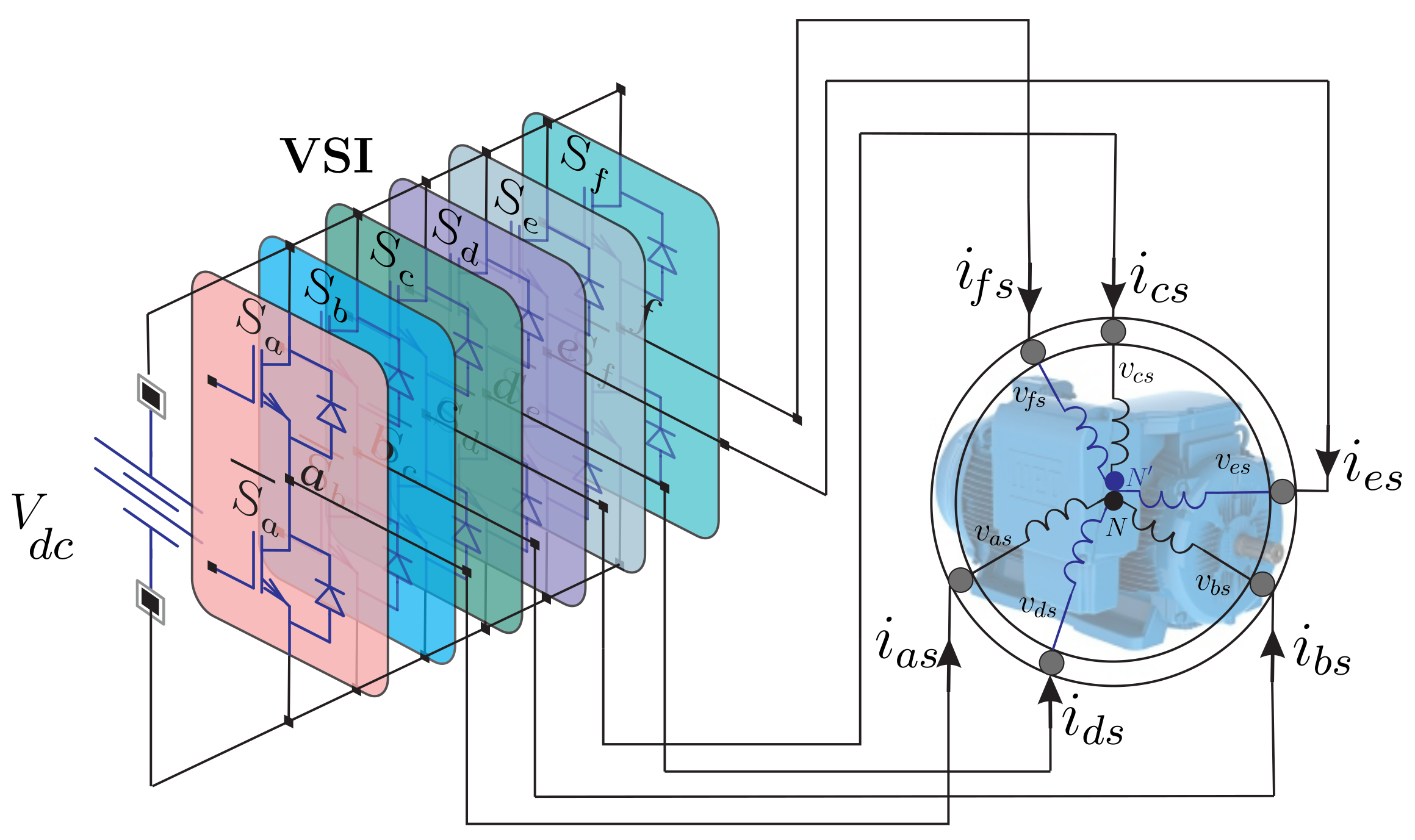
2. SPIM State-Space Model
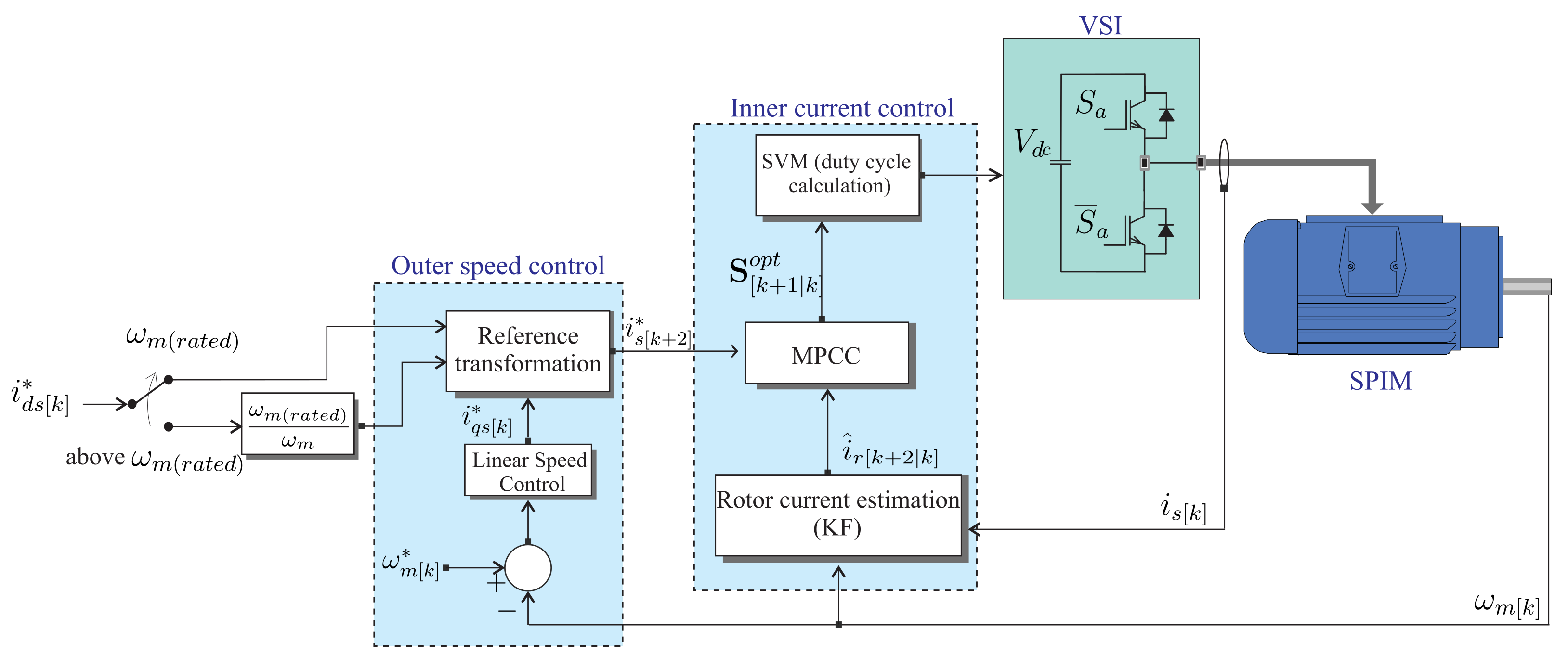
3. Proposed Control Applied to the SPIM
3.1. Rotor Speed Control
3.2. PCC Based on FCS-MPC
3.3. Rotor Current Observers
3.4. Cost Function
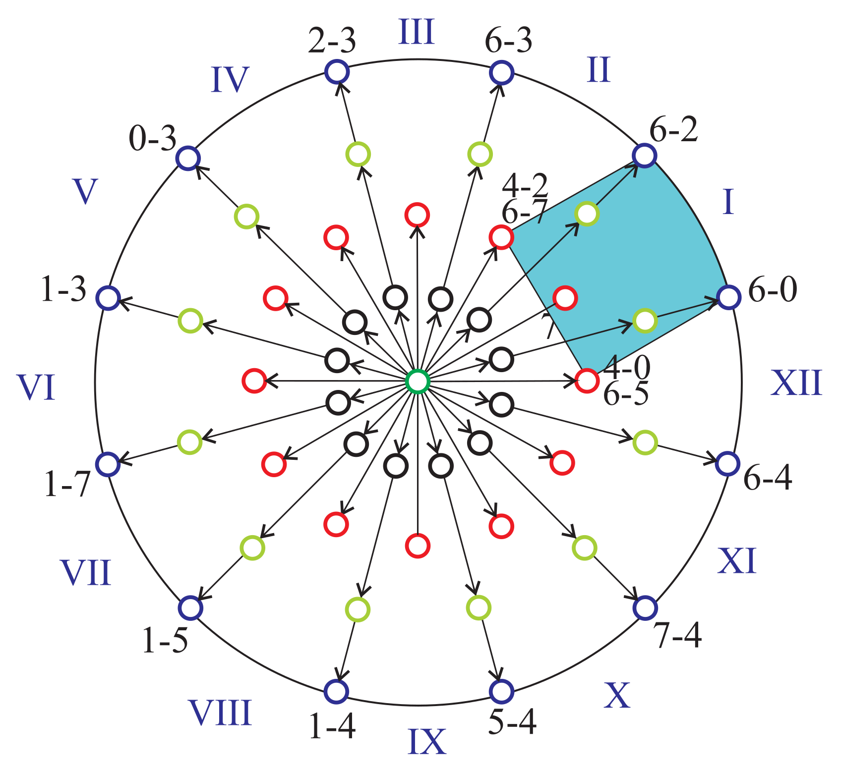
3.5. Modulated PCC (MPCC)
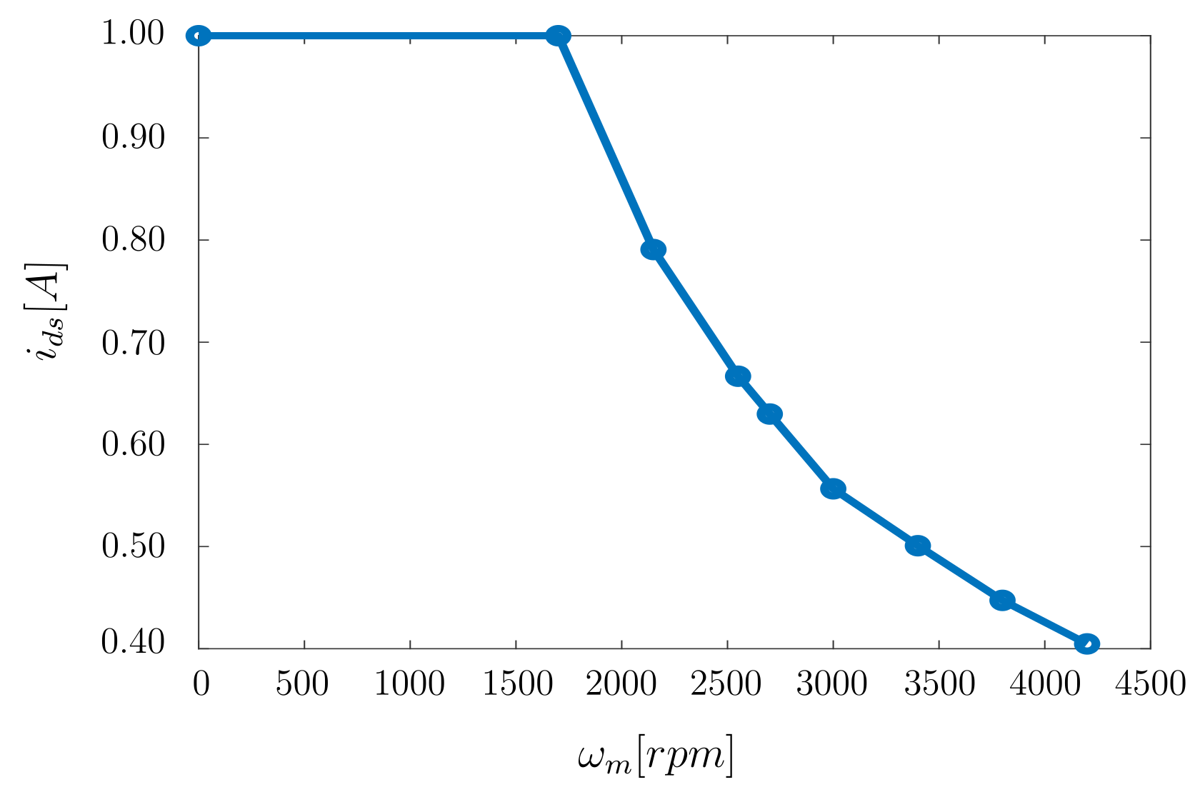
3.6. Field-Weakening Operation Applied with MPCC
4. Experimental Results
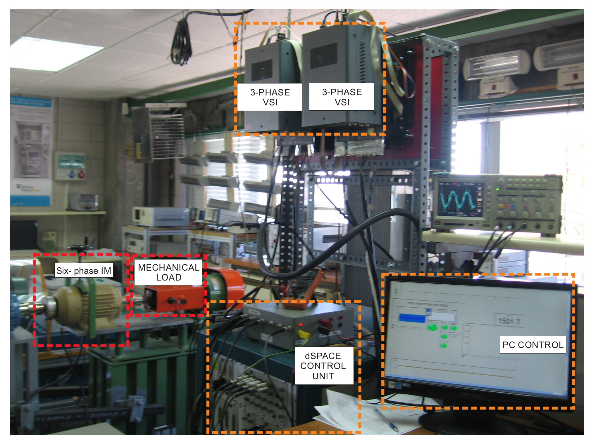
4.1. Experimental Bench Composition
4.2. Figures of Merit
4.3. Steady-State Results
4.4. Transient Results
4.5. Robustness Results
4.6. Comparative Analysis
5. Conclusions
Author Contributions
Funding
Institutional Review Board Statement
Informed Consent Statement
Data Availability Statement
Acknowledgments
Conflicts of Interest
Abbreviations
| FCS-MPC | Finite control version of model predictive control |
| FOC | Field-oriented control |
| FW | Field weakening |
| IGBT | Isolated gate bipolar transistor |
| IRFOC | Indirect rotor field-oriented control |
| KF | Kalman filter |
| LO | Luenberger observer |
| LV | Large vector |
| MV | Mid vector |
| MPCC | Modulated predictive control |
| MSE | Mean square error |
| PCC | Predictive current control |
| PI | Proportional-integral |
| SPIM | Six-phase induction machine |
| SVM | Space vector modulation |
| THD | Total harmonic distortion |
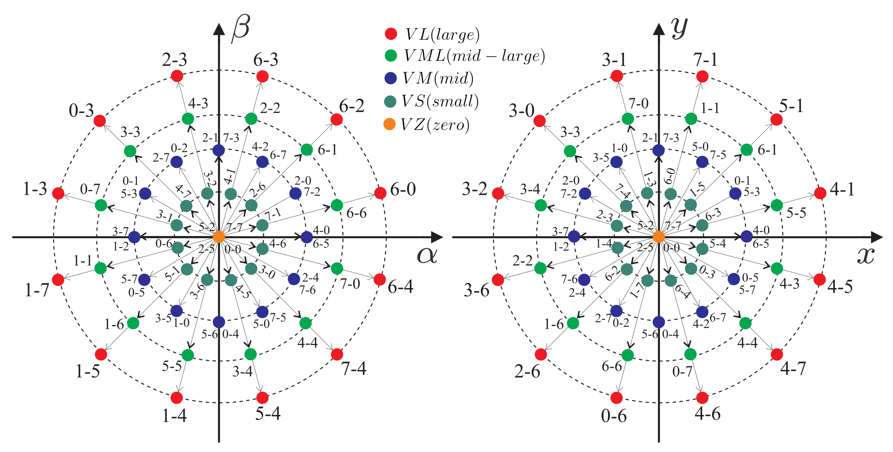
| VSD | Vector space decomposition |
| VSI | Voltage source inverter |
| ZV | Null vector |
References
- Levi, E. Advances in Converter Control and Innovative Exploitation of Additional Degrees of Freedom for Multiphase Machines. IEEE Trans. Ind. Electron. 2016, 63, 433–448. [Google Scholar] [CrossRef]
- Barrero, F.; Duran, M.J. Recent Advances in the Design, Modeling, and Control of Multiphase Machines: Part I. IEEE Trans. Ind. Electron. 2016, 63, 449–458. [Google Scholar] [CrossRef]
- Liu, Z.; Li, Y.; Zheng, Z. A review of drive techniques for multiphase machines. CES Trans. Electr. Mach. Syst. 2018, 2, 243–251. [Google Scholar] [CrossRef]
- Duran, M.J.; Barrero, F. Recent Advances in the Design, Modeling, and Control of Multiphase Machines: Part II. IEEE Trans. Ind. Electron. 2016, 63, 459–468. [Google Scholar] [CrossRef]
- Peng, X.; Liu, Z.; Jiang, D. A review of multiphase energy conversion in wind power generation. Renew. Sustain. Energy Rev. 2021, 147, 111172. [Google Scholar] [CrossRef]
- Prieto, I.G.; Duran, M.J.; Garcia-Entrambasaguas, P.; Bermudez, M. Field-oriented control of multiphase drives with passive fault tolerance. IEEE Trans. Ind. Electron. 2019, 67, 7228–7238. [Google Scholar] [CrossRef]
- Heidari, H.; Rassõlkin, A.; Vaimann, T.; Kallaste, A.; Taheri, A.; Holakooie, M.H.; Belahcen, A. A novel vector control strategy for a six-phase induction motor with low torque ripples and harmonic currents. Energies 2019, 12, 1102. [Google Scholar] [CrossRef]
- Holakooie, M.H.; Iwanski, G.; Miazga, T. Switching-Table-Based Direct Torque Control of Six-Phase Drives With xy Current Regulation. IEEE Trans. Ind. Electron. 2022, 69, 11890–11902. [Google Scholar] [CrossRef]
- Zaidi, E.; Marouani, K.; Bouadi, H.; Nounou, K.; Aissani, M.; Bentouhami, L. Control of a multiphase machine fed by multilevel inverter based on sliding mode controller. In Proceedings of the 2019 IEEE International Conference on Environment and Electrical Engineering and 2019 IEEE Industrial and Commercial Power Systems Europe (EEEIC/I&CPS Europe), Genova, Italy, 11–14 June 2019; pp. 1–6. [Google Scholar] [CrossRef]
- Mossa, M.A.; Echeikh, H.; El Ouanjli, N.; Alhelou, H.H. Enhanced Second-Order Sliding Mode Control Technique for a Five-Phase Induction Motor. Int. Transact. Electr. Energy Syst. 2022, 2022, 8215525. [Google Scholar] [CrossRef]
- Rodriguez, J.; Garcia, C.; Mora, A.; Flores-Bahamonde, F.; Acuna, P.; Novak, M.; Zhang, Y.; Tarisciotti, L.; Davari, S.A.; Zhang, Z.; et al. Latest advances of model predictive control in electrical drives—Part I: Basic concepts and advanced strategies. IEEE Trans. Power Electron. 2021, 37, 3927–3942. [Google Scholar] [CrossRef]
- Duran, M.J.; Gonzalez-Prieto, I.; Gonzalez-Prieto, A.; Aciego, J.J. The Evolution of Model Predictive Control in Multiphase Electric Drives: A Growing Field of Research. IEEE Ind. Electron. Mag. 2022, 16, 29–39. [Google Scholar] [CrossRef]
- Gonzalez-Prieto, I.; Duran, M.J.; Aciego, J.J.; Martin, C.; Barrero, F. Model predictive control of six-phase induction motor drives using virtual voltage vectors. IEEE Trans. Ind. Electron. 2017, 65, 27–37. [Google Scholar] [CrossRef]
- Aciego, J.J.; Prieto, I.G.; Duran, M.J. Model predictive control of six-phase induction motor drives using two virtual voltage vectors. IEEE J. Emerg. Sel. Top. Power Electron. 2018, 7, 321–330. [Google Scholar] [CrossRef]
- González-Prieto, I.; Durán, M.; Bermúdez, M.; Barrero, F.; Martín, C. Assessment of Virtual-Voltage-based Model Predictive Controllers in Six-phase Drives under Open-Phase Faults. IEEE J. Emerg. Sel. Top. Power Electron. 2019, 8, 2634–2644. [Google Scholar] [CrossRef]
- Ayala, M.; Doval-Gandoy, J.; Rodas, J.; Gonzalez, O.; Gregor, R.; Rivera, M. A novel modulated model predictive control applied to six-phase induction motor drives. IEEE Trans. Ind. Electron. 2020, 68, 3672–3682. [Google Scholar] [CrossRef]
- Sharma, S.; Aware, M.V.; Bhowate, A. Symmetrical six-phase induction motor-based integrated driveline of electric vehicle with predictive control. IEEE Trans. Transp. Electrif. 2020, 6, 635–646. [Google Scholar] [CrossRef]
- Arahal, M.R.; Barrero, F.; Satué, M.G.; Ramírez, D.R. Predictive Control of Multi-Phase Motor for Constant Torque Applications. Machines 2022, 10, 211. [Google Scholar] [CrossRef]
- Zarri, L.; Mengoni, M.; Tani, A.; Serra, G.; Casadei, D.; Ojo, J. Control schemes for field weakening of induction machines: A review. In Proceedings of the 2015 IEEE Workshop on Electrical Machines Design, Control and Diagnosis (WEMDCD), Turin, Italy, 26–27 March 2015; pp. 146–155. [Google Scholar] [CrossRef]
- Kim, S.H.; Sul, S.K. Maximum torque control of an induction machine in the field weakening region. IEEE Trans. Ind. Appl. 1995, 31, 787–794. [Google Scholar] [CrossRef]
- Su, J.; Gao, R.; Husain, I. Model predictive control based field-weakening strategy for traction—EV used induction motor. IEEE Trans. Ind. Appl. 2017, 54, 2295–2305. [Google Scholar] [CrossRef]
- Zhang, Y.; Zhang, B.; Yang, H.; Norambuena, M.; Rodriguez, J. Generalized sequential model predictive control of IM drives with field-weakening ability. IEEE Trans. Power Electron. 2018, 34, 8944–8955. [Google Scholar] [CrossRef]
- Xu, W.; Tang, Y.; Dong, D.; Xiao, X.; Rashad, E.E.M.; Junejo, A.K. Optimal reference primary flux based model predictive control of linear induction machine with MTPA and field-weakening operations for urban transit. IEEE Trans. Ind. Appl. 2022, 58, 4708–4721. [Google Scholar] [CrossRef]
- Ayala, M.; Doval-Gandoy, J.; Gonzalez, O.; Rodas, J.; Gregor, R.; Rivera, M. Experimental stability study of modulated model predictive current controllers applied to six-phase induction motor drives. IEEE Trans. Power Electron. 2021, 36, 13275–13284. [Google Scholar] [CrossRef]
- Xu, X.; Novotny, D.W. Selection of the flux reference for induction machine drives in the field weakening region. IEEE Trans. Ind. Appl. 1992, 28, 1353–1358. [Google Scholar] [CrossRef]
- Zhao, Y.; Lipo, T. Space vector PWM control of dual three-phase induction machine using vector space decomposition. IEEE Trans. Ind. Electron. 1995, 31, 1100–1109. [Google Scholar] [CrossRef]
- Harnefors, L.; Saarakkala, S.E.; Hinkkanen, M. Speed control of electrical drives using classical control methods. IEEE Trans. Ind. Appl. 2013, 49, 889–898. [Google Scholar] [CrossRef]
- Martin, C.; Arahal, M.; Barrero, F.; Duran, M. Five-Phase Induction Motor Rotor Current Observer for Finite Control Set Model Predictive Control of Stator Current. IEEE Trans. Ind. Electron. 2016, 63, 4527–4538. [Google Scholar] [CrossRef]
- Wang, B.; Luo, C.; Yu, Y.; Wang, G.; Xu, D. Antidisturbance speed control for induction machine drives using high-order fast terminal sliding-mode load torque observer. IEEE Trans. Power Electron. 2017, 33, 7927–7937. [Google Scholar] [CrossRef]
- Yang, Z.; Zhang, D.; Sun, X.; Ye, X. Adaptive exponential sliding mode control for a bearingless induction motor based on a disturbance observer. IEEE Access 2018, 6, 35425–35434. [Google Scholar] [CrossRef]
- Rodas, J.; Barrero, F.; Arahal, M.R.; Martín, C.; Gregor, R. Online estimation of rotor variables in predictive current controllers: A case study using five-phase induction machines. IEEE Trans. Ind. Electron. 2016, 63, 5348–5356. [Google Scholar] [CrossRef]
- Novak, M.; Dragicevic, T.; Blaabjerg, F. Weighting factor design based on Artificial Neural Network for Finite Set MPC operated 3L-NPC converter. In Proceedings of the 2019 IEEE Applied Power Electronics Conference and Exposition (APEC), Anaheim, CA, USA, 17–21 March 2019; pp. 77–82. [Google Scholar] [CrossRef]
- Majmunović, B.; Dragičević, T.; Blaabjerg, F. Multi Objective Modulated Model Predictive Control of Stand-Alone Voltage Source Converters. IEEE J. Emerg. Sel. Top. Power Electron. 2019, 8, 2559–2571. [Google Scholar] [CrossRef]
- Van Der Broeck, H.W.; Skudelny, H.C.; Stanke, G.V. Analysis and realization of a pulsewidth modulator based on voltage space vectors. IEEE Trans. Ind. Appl. 1988, 24, 142–150. [Google Scholar] [CrossRef]
- Riveros, J.A.; Yepes, A.G.; Barrero, F.; Doval-Gandoy, J.; Bogado, B.; Lopez, O.; Jones, M.; Levi, E. Parameter identification of multiphase induction machines with distributed windings—Part II: Time-domain techniques. IEEE Trans. Energy Conv. 2012, 27, 1067–1077. [Google Scholar] [CrossRef]
- Wang, F.; Zhang, Z.; Mei, X.; Rodríguez, J.; Kennel, R. Advanced control strategies of induction machine: Field oriented control, direct torque control and model predictive control. Energies 2018, 11, 120. [Google Scholar] [CrossRef]
- Gonzalez, O.; Ayala, M.; Doval-Gandoy, J.; Rodas, J.; Gregor, R.; Rivera, M. Predictive-Fixed Switching Current Control Strategy Applied to Six-Phase Induction Machine. Energies 2019, 12, 2294. [Google Scholar] [CrossRef]
- Gonzalez, O.; Ayala, M.; Romero, C.; Delorme, L.; Rodas, J.; Gregor, R.; Gonzalez-Prieto, I.; Durán, M.J. Model predictive current control of six-phase induction motor drives using virtual vectors and space vector modulation. IEEE Trans. Power Electron. 2022, 37, 7617–7628. [Google Scholar] [CrossRef]


| Parameter | Value | Parameter | Value |
|---|---|---|---|
| () | 6.9 | () | 6.7 |
| (mH) | 654.4 | (mH) | 626.8 |
| (mH) | 614 | (mH) | 5.3 |
| (r/min) | 2540 | (kW) | 2 |
| (kg·) | 0.07 | (kg·/s) | 0.0004 |
| P | 1 | 0.1533 | |
| (Nm) | 7.5 | (A) | 2.2 |
| 1700 | 0.0973 | 0.1076 | 0.2011 | 0.2033 | 4.44 |
| 2150 | 0.1497 | 0.1593 | 0.2291 | 0.2305 | 3.98 |
| 2550 | 0.1359 | 0.1461 | 0.2527 | 0.2476 | 3.98 |
| 1700 | 10.57 | 11.95 | 0.0792 | 0.1216 | |
| 2150 | 11.88 | 12.24 | 0.0793 | 0.2037 | |
| 2550 | 7.82 | 8.18 | 0.0743 | 0.1852 |
| 2150 | 0.1618 | 0.1608 | 0.2352 | 0.2311 | 3.50 |
| 2550 | 0.1237 | 0.1287 | 0.2325 | 0.2373 | 3.36 |
| 3000 | 0.1912 | 0.1957 | 0.2755 | 0.2700 | 4.27 |
| 3400 | 0.1773 | 0.1796 | 0.2828 | 0.2763 | 8.54 |
| 3800 | 0.1702 | 0.1724 | 0.1924 | 0.1929 | 6.26 |
| 4200 | 0.1642 | 0.1693 | 0.1976 | 0.2019 | |
| 2150 | 10.77 | 11.13 | 0.0912 | 0.2091 | |
| 2550 | 7.45 | 8.10 | 0.1104 | 0.1402 | |
| 3000 | 6.48 | 6.90 | 0.1593 | 0.2224 | |
| 3400 | 5.07 | 5.11 | 0.1936 | 0.1619 | |
| 3800 | 22.96 | 22.73 | 0.0988 | 0.2211 | |
| 4200 | 23.44 | 23.93 | 0.1029 | 0.2122 |
| of rated | |||||
|---|---|---|---|---|---|
| 2550 | 0.1750 | 0.1758 | 0.2592 | 0.2503 | 3.93 |
| 2550 | 9.68 | 9.64 | 0.0765 | 0.2360 | |
| of rated | |||||
| 2550 | 0.1712 | 0.1762 | 0.2578 | 0.2515 | 4.09 |
| 2550 | 8.83 | 9.08 | 0.0728 | 0.2347 | |
| of rated | |||||
|---|---|---|---|---|---|
| 2550 | 0.1804 | 0.1800 | 0.2561 | 0.2541 | 4.05 |
| 2550 | 8.74 | 9.04 | 0.1140 | 0.2279 | |
| of rated | |||||
| 2550 | 0.1622 | 0.1642 | 0.2534 | 0.2472 | 4.24 |
| 2550 | 8.63 | 8.96 | 0.1088 | 0.2035 | |
| 2150 | 0.1765 | 0.1837 | 0.1668 | 0.1689 | 2.5662 |
| 2550 | 0.2400 | 0.2447 | 0.1885 | 0.1932 | 2.4694 |
| 3000 | 0.3552 | 0.3574 | 0.2207 | 0.2296 | 3.6711 |
| 3400 | 0.4119 | 0.4102 | 0.2331 | 0.2430 | 227.28 |
| 2150 | 11.07 | 12.67 | 0.1503 | 0.2057 | |
| 2550 | 10.34 | 11.06 | 0.2285 | 0.2555 | |
| 3000 | 9.82 | 9.83 | 0.3693 | 0.3429 | |
| 3400 | 9.13 | 9.43 | 0.4415 | 0.3781 |
| 2150 | 0.1692 | 0.1762 | 0.1251 | 0.1267 | 2.2272 |
| 2550 | 0.2580 | 0.2633 | 0.1397 | 0.1429 | 2.1261 |
| 3000 | 0.3859 | 0.3883 | 0.1591 | 0.1651 | 3.0635 |
| 3400 | 0.4529 | 0.4505 | 0.1634 | 0.1702 | 223.54 |
| 2150 | 10.46 | 11.15 | 0.1616 | 0.2214 | |
| 2550 | 11.02 | 12.13 | 0.2485 | 0.2776 | |
| 3000 | 10.92 | 11.03 | 0.4059 | 0.3765 | |
| 3400 | 10.22 | 10.45 | 0.4908 | 0.4198 |
Disclaimer/Publisher’s Note: The statements, opinions and data contained in all publications are solely those of the individual author(s) and contributor(s) and not of MDPI and/or the editor(s). MDPI and/or the editor(s) disclaim responsibility for any injury to people or property resulting from any ideas, methods, instructions or products referred to in the content. |
© 2024 by the authors. Licensee MDPI, Basel, Switzerland. This article is an open access article distributed under the terms and conditions of the Creative Commons Attribution (CC BY) license (https://creativecommons.org/licenses/by/4.0/).
Share and Cite
Ayala, M.; Doval-Gandoy, J.; Rodas, J.; Gonzalez, O.; Gregor, R.; Delorme, L.; Romero, C.; Fleitas, A. Field-Weakening Strategy with Modulated Predictive Current Control Applied to Six-Phase Induction Machines. Machines 2024, 12, 178. https://doi.org/10.3390/machines12030178
Ayala M, Doval-Gandoy J, Rodas J, Gonzalez O, Gregor R, Delorme L, Romero C, Fleitas A. Field-Weakening Strategy with Modulated Predictive Current Control Applied to Six-Phase Induction Machines. Machines. 2024; 12(3):178. https://doi.org/10.3390/machines12030178
Chicago/Turabian StyleAyala, Magno, Jesus Doval-Gandoy, Jorge Rodas, Osvaldo Gonzalez, Raúl Gregor, Larizza Delorme, Carlos Romero, and Ariel Fleitas. 2024. "Field-Weakening Strategy with Modulated Predictive Current Control Applied to Six-Phase Induction Machines" Machines 12, no. 3: 178. https://doi.org/10.3390/machines12030178
APA StyleAyala, M., Doval-Gandoy, J., Rodas, J., Gonzalez, O., Gregor, R., Delorme, L., Romero, C., & Fleitas, A. (2024). Field-Weakening Strategy with Modulated Predictive Current Control Applied to Six-Phase Induction Machines. Machines, 12(3), 178. https://doi.org/10.3390/machines12030178