Design and Development of a Brake Test Bench for Formula SAE Race Cars

Abstract

The optimization of the brake systems is crucial for vehicle performance and safety of Formula SAE (FSAE) race cars. This study introduces a specialized brake test bench designed to enhance the understanding and testing of these systems. The bench integrates a rotating mechanical system mounting a brake disc-caliper group, which is driven by an electric motor, a pneumatic brake pedal assembly to simulate real braking conditions, and a comprehensive array of sensors that facilitate the measurement of critical parameters, such as rotation speed, braking torque, oil pressure, and disc temperature. Its structure, sensor integration, and control electronics are fully described, demonstrating the capability to replicate on-track scenarios in a controlled environment. The results underscore the utility of the bench in providing precise and consistent testing conditions essential for analyzing the efficiency, durability, and safety of the braking systems of FSAE race cars.

1. Introduction

Formula SAE^® is a series of competitions in which different teams of university undergraduate and graduate students compete to design, construct, test, and promote a race car prototype that adheres to stringent regulations [1] and mimics real-world racing standards. The present work underscores the importance of the brake system in these high-performance vehicles [2,3,4,5], which are subject to intense engineering scrutiny and competitive performance. Traditional design and testing methods fall short, particularly since the brake system can typically only be evaluated after the entire vehicle is assembled, leading to potential issues being discovered too late in the development process [6].

Over the years, the need to overcome these limitations has suggested the adoption of laboratory brake testing devices, which are superior in efficiency and control to vehicle testing, as they involve fewer variables and reduced testing and engineering resources [7]. Numerous test systems have been proposed and adopted in the automotive sector (but also in other sectors, for example, railways [8,9,10]), each distinguished by the test procedures, experimental setups, and samples they adopt [11]. Generally, testing machines can be categorized into three main types based on whether the experimental tests are conducted using a pin-on-disc (or block-on-ring) configuration [12,13,14,15,16], a brake dynamometer (also called inertia dynamometer) [17,18], or a roller chassis bench (also called chassis dynamometer) [6,19]. Clear and useful overviews of the main testing systems, along with a concise history of the development of automotive brake test systems, are available in [20,21].

Despite the wide range of dynamometers already available, the need for designing and building a dynamometer dedicated to FSAE cars is two-fold. The first and most important concern is the size of the machines. For an FSAE car’s brake system, commercial dynamometers are generally quite oversized since they are designed for road vehicles. To clarify this point, consider that standard cars are designed to last hundreds of thousands of kilometers and to travel at cruising speeds of up to 130 km/h or even more. As a result, the smallest commercial inertia dynamometers are designed to test brake systems with maximum rotational speeds of up to about 300 rad/s, simulate inertias ranging from tens to thousands of kg∙m², apply braking torques in the order of 2000–5000 Nm, and supply the brake line with pressures even higher than 200 bar. It will be shown in the following section that these values are out of scale compared to those of a FSAE car, which are quite lighter and typically meant to cover at most a few thousand kilometers with a maximum speed of about 90 km/h. The second reason, more trivial, is identified in the cost of the machinery, which clearly follows the size of the machine.

Nevertheless, besides the size or the costs of the selected setup, another reason justifying the need for developing a brake test bench dedicated exclusively to FSAE cars concerns the operating mode of the bench and the adopted test protocols. Noteworthily, considerable effort has been invested in creating guidelines to minimize variability and enhance the correlation between dynamometer and vehicle test results. Indeed, factors like the measuring system (dynamometer and test setup) and the methodology (laboratory procedures, data gathering, and reporting), along with variations in the friction pair (both within and across production batches of friction materials and rotors), significantly affect the consistency and range of the brake parameters measured during a specific test (or sequence of tests), e.g., the friction coefficient [7,22]. This aspect, as well as the need to homologate mass-produced braking systems with increasingly larger volumes, has made it progressively necessary to define appropriate standardized test protocols to perform repeatable measurements at very low time and cost [7,11,20,22]. As a result, numerous standards (e.g., [23,24,25,26,27,28,29]) have been established, each marked by rigorous testing protocols that define a sequence of braking runs, regulated by pressure or deceleration, across various conditions (including braking and release speeds, pressure or deceleration levels, and brake temperature).

While the use of standards provides a benchmark for repeatable and objective assessments and ensures a standardized level of safety and quality, on the other hand, it may prove inadequate or even restrictive for racing, which often demands customized and generally higher performance and specifications compared to standard vehicles. In fact, racing components are designed to maximize performance in a specific track or test (e.g., brake test, autocross, or endurance for FSAE cars [1]), often sacrificing cost-effectiveness, durability, and other features (which are essential in standard vehicles).

Consequently, there is a need to develop equipment and testing protocols specific to the sector that consider the unique requirements and allow for the study of the braking system’s performance in light of its real operating conditions.

There are some examples in the literature of brake test benches specifically designed and built for FSAE cars. For instance, the authors in [2] proposed an experimental setup that mimics the entire braking system of the car, including the pedal assembly. However, it is limited to tests of the pedal assembly and the pipeline since it has a stationary brake disc. Other authors have developed dynamic systems dedicated to FSAE vehicles by adapting a commercial dynamometer [30] or creating a new dynamometer from scratch [3]. However, the proposed systems are limited to braking at constant speed and pressure or according to standard test protocols and regulations [3,30].

In other words, as far as the authors know, there are no dynamometers for FSAE vehicles in the literature that accurately reproduce the entire braking system of the car under real operating conditions. Accordingly, this work sets out to overcome these challenges by creating a brake test bench that allows for earlier and more detailed testing of the brake system for FSAE cars. More in detail, the present contribution describes a comprehensive study on the design, development, and testing of a brake test bench tailored for Formula SAE race cars and conceived to replicate the real-world conditions the car’s braking system would undergo during races. The proposed brake test bench can faithfully replicate both the entire braking system (from disc, pad, and caliper to tubing, pump, and pedal assembly) and the real operating conditions experienced in the track. This enables the testing and comparison of different brake disc-caliper combinations and friction pairs under non-standard operating conditions, such as those derived from actual track data. It can also allow for the study of the brake system’s thermal regime under realistic operational loads, making it possible to compare and validate analytical/numerical models (as undertaken, for example, in [30] for a simple load history). Eventually, it permits evaluating and verifying the structural durability and fatigue strength of new non-commercial engineering solutions for the braking system, studying fading behavior and wear mechanisms, or investigating the differences in pedal feedback under various loading conditions.

In what follows, a detailed examination will be given of the brake test bench’s concept, followed by an in-depth analysis of the main components and electronic control system. Eventually, attention will be directed towards replicating the on-track conditions on the test bench, focusing particularly on the velocity profile and the brake disc temperature profile.

2. The Brake Test Bench: Concept and Overview

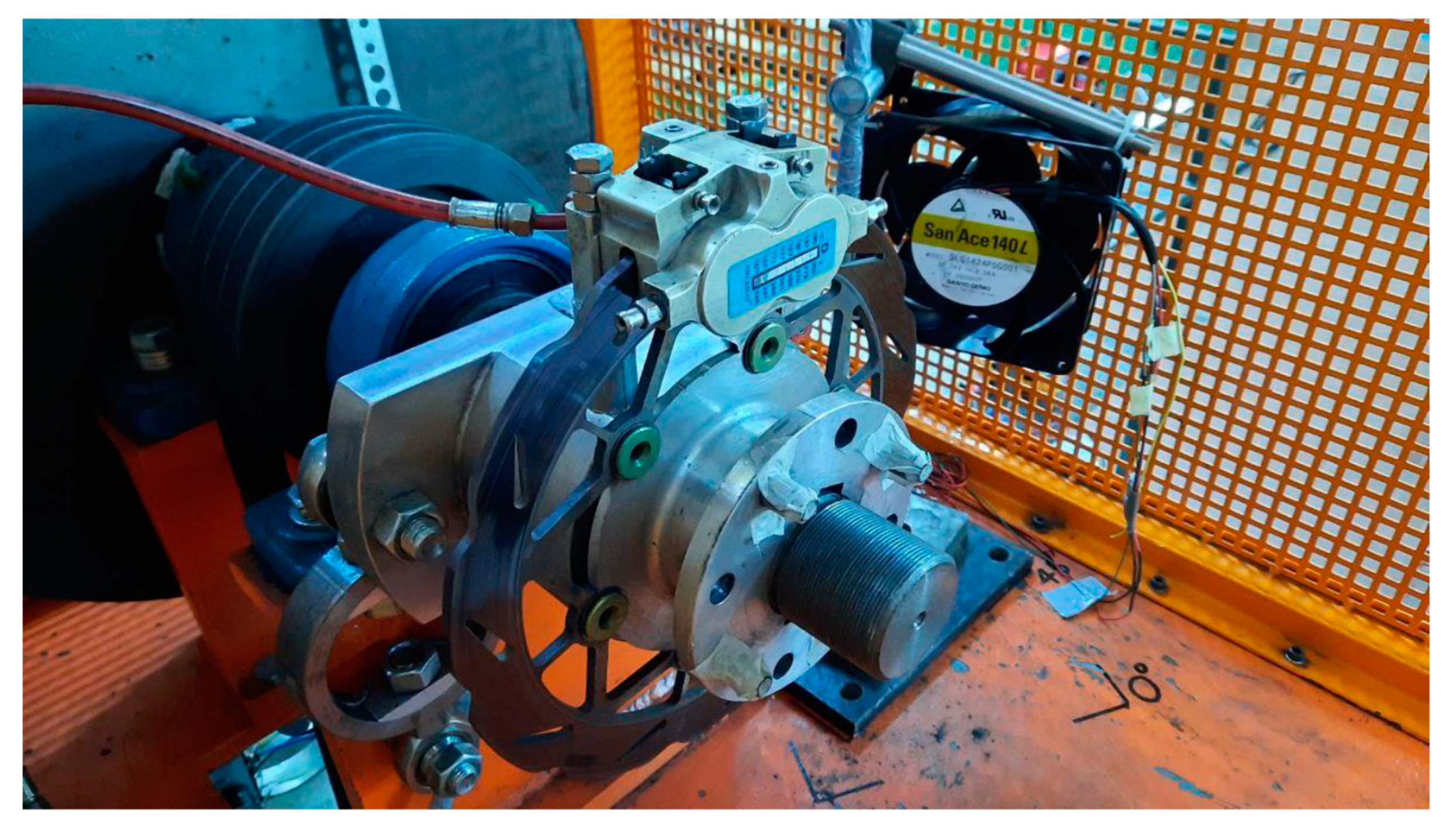
The brake test bench is a complex assembly of mechanical and electronic systems, including moving mechanical components, a pneumatic actuation system, a powered electrical line, and a sensor network connected to a single electronic control system running LabView code. A schematic and essential representation of the brake test bench is shown in Figure 1, while some images of the actual bench are provided in Figure 2.

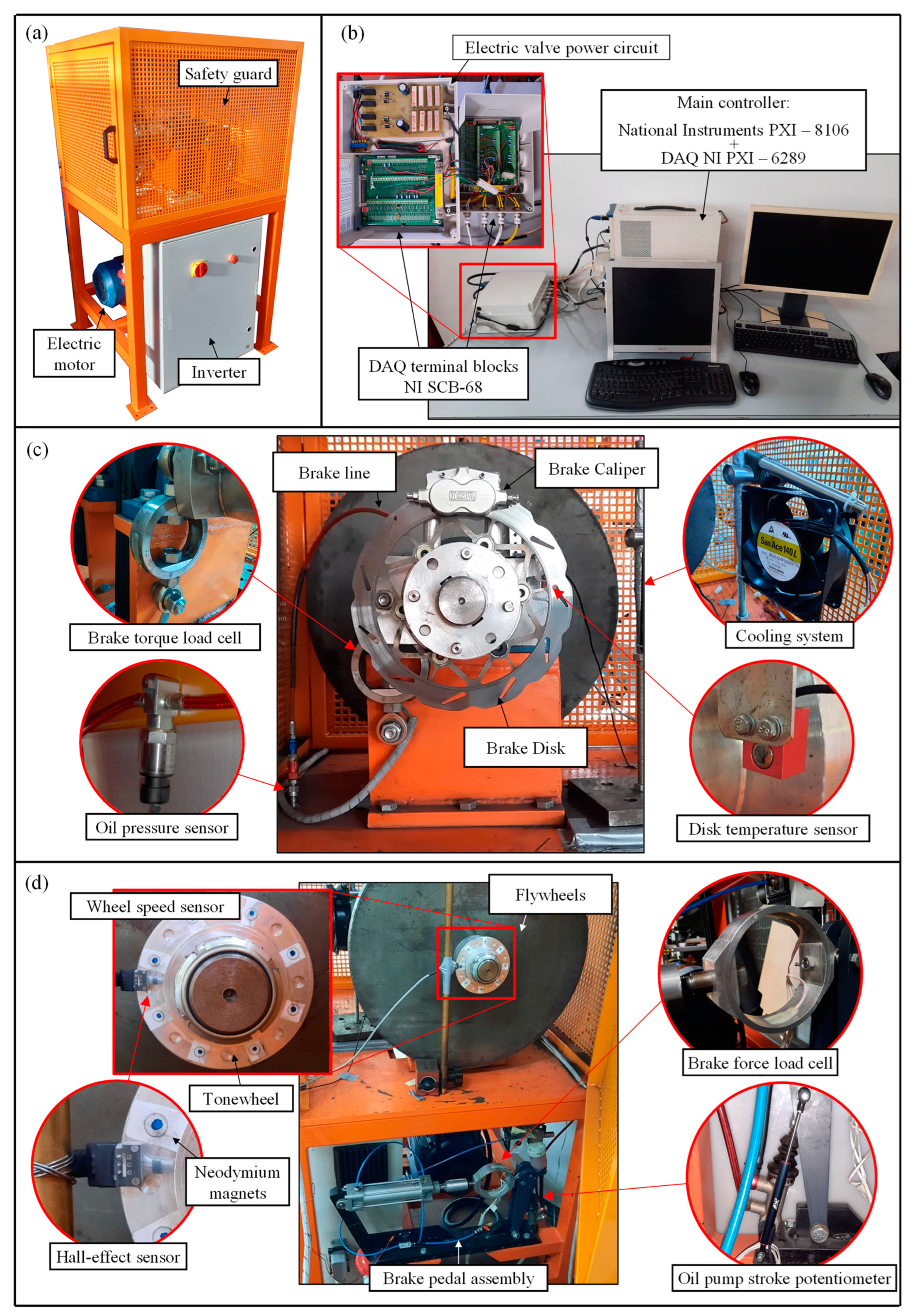
The operating principle of the brake test bench is very straightforward: a brake disc is installed and allowed to float on a rotating shaft, which is accelerated by an electric motor and decelerated by a brake caliper attached to the bench’s frame (Figure 1). In more detail, the system consists of a steel tubular structure (Figure 2a) to which the rotating shaft is attached via two ball bearings. Its rotation is permitted by a belt drive system powered by a three-phase asynchronous electric motor (Figure 1), which is controlled by a dedicated electronic control system (Figure 2b). The bench is equipped with a series of flywheels (in varying numbers as needed) that accumulate kinetic energy to be dissipated during the braking phase, simulating the vehicle’s inertia. As mentioned, this braking is made possible by the presence of the brake caliper (Figure 2c), which is connected to the frame and operated by a braking system with a pedal and brake pump similar to that of a real vehicle (Figure 2d).

The concept of the main components of the bench, such as the flywheel mass and electric motor, was aimed at replicating the most severe braking conditions encountered in the car, i.e., in the case of the highest initial speed and deceleration. Accordingly, the first step was to assess the maximum kinetic energy stored by the individual front wheel group, as this is the most stressed due to load transfer:

$$E_{\mathrm{K},\mathrm{F},max}=\frac{1}{2}{m}_{\mathrm{F},max}{v}_{max}^2$$

(1)

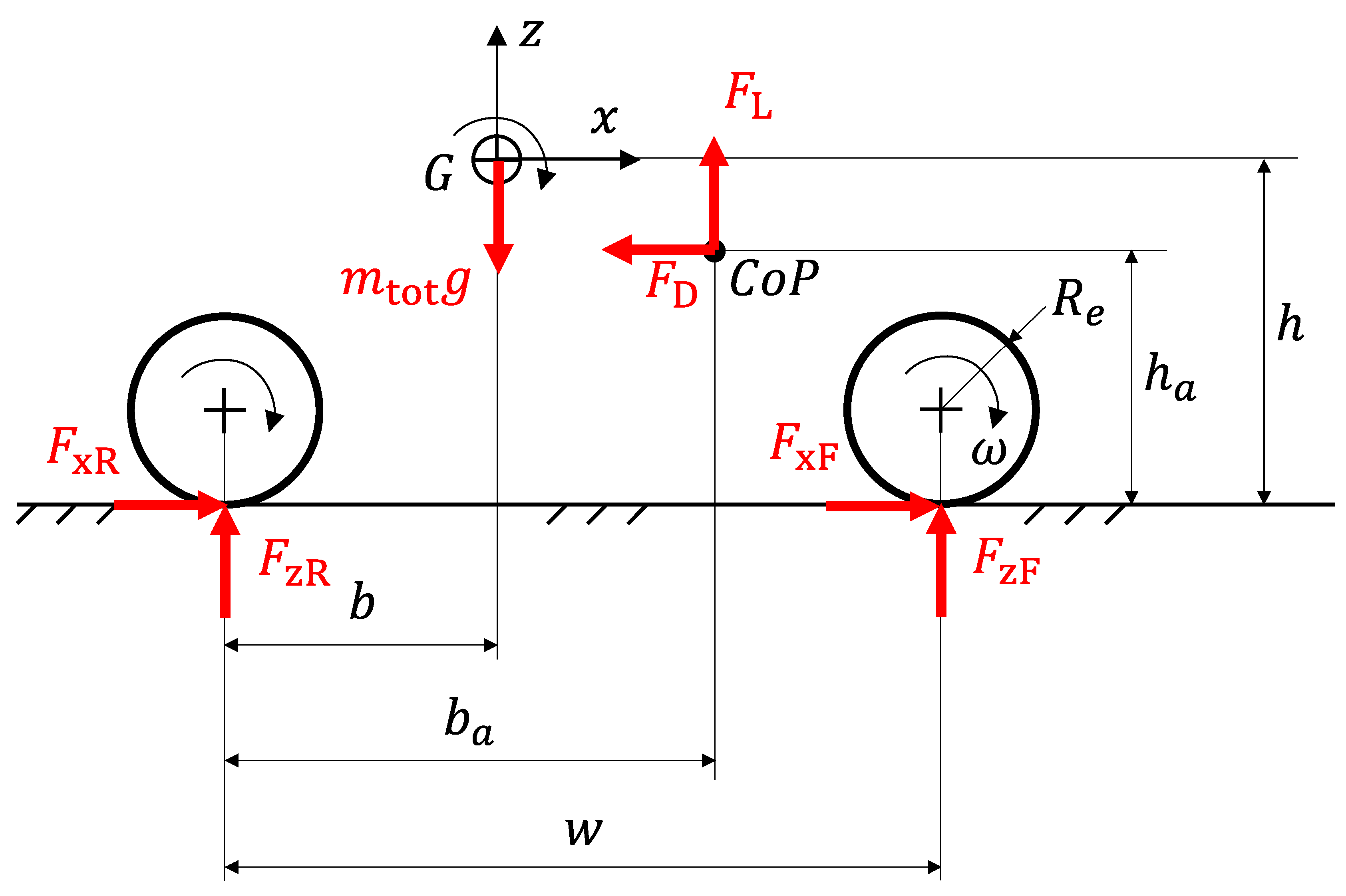
where $m_{\mathrm{F},max}$ is the maximum value of the car’s mass that is transferred to each front wheel group during braking, and $v_{max}$ is the maximum speed of the car. Assuming a flat track, a symmetric car, and symmetry of loads in the pitch plane (perfectly straight accelerations and braking), an effective estimate of $m_{\mathrm{F},max}$ can be made using the model shown in Figure 3.

In this model, the vehicle and driver are represented by a point mass m_tot at the overall center of mass G. This is located at a distance b and a height h from the rear wheel contact point, while the center of pressure, i.e., the point of application of the resultant aerodynamic lift and drag forces, is at the coordinates (b_a,h_a). The wheelbase of the vehicle is w. The external forces acting on the vehicle are the drag force F_D, the lift force F_L, the weight m_tot∙g and the forces exchanged by the tires with the ground in the pitch plane, i.e., F_xR, F_zR, F_xF, and F_zF (the latter, given the symmetry of the problem, are twice the force exchanged by each of the tires with the ground).

With reference to the schematic in Figure 3, the following motion equations can be written [31]:

$$\left\{\begin{array}{c}{F}_{\mathrm{x}\mathrm{R}}+F_{\mathrm{x}\mathrm{F}}-F_{\mathrm{D}}=m_{\mathrm{t}\mathrm{o}\mathrm{t}}{\ddot{x}}_{\mathrm{G}} \\ F_{\mathrm{z}\mathrm{R}}+F_{\mathrm{z}\mathrm{F}}-m_{\mathrm{t}\mathrm{o}\mathrm{t}}g+F_{\mathrm{L}}=0 \\ b{F}_{\mathrm{z}\mathrm{R}}-\left(w-b\right)F_{\mathrm{z}\mathrm{F}}-h\left(F_{\mathrm{x}\mathrm{R}}+F_{\mathrm{x}\mathrm{F}}\right)+\left(h-h_a\right)F_{\mathrm{D}}-(b_a-b)F_{\mathrm{L}}=I_{\mathrm{F}}{\ddot{\theta }}_{\mathrm{F}}+I_{\mathrm{R}}{\ddot{\theta }}_{\mathrm{R}}\pm I_e{\ddot{\theta }}_e\hfill \end{array}\right.$$

(2)

where ${\ddot{x}}_G$ is the longitudinal acceleration of the vehicle; I_F, I_R, and I_e are the moment of inertia of the front axle, the rear axle, and the set of rotating parts belonging to the engine reduced to the transmission shaft, respectively, while ${\ddot{\theta }}_{\mathrm{F}}, {\ddot{\theta }}_{\mathrm{R}}$, and ${\ddot{\theta }}_e$ are their respective angular accelerations. After rearranging the first two equations and substituting them into the third, it is possible to explicitly calculate the value of the force F_zF as follows:

$$F_{\mathrm{z}\mathrm{F}}=m_{\mathrm{t}\mathrm{o}\mathrm{t}} g\frac{b}{w}-m_{\mathrm{t}\mathrm{o}\mathrm{t}}{\ddot{x}}_{\mathrm{G}}\frac{h}{w}-F_{\mathrm{D}}\frac{h_a}{w}-F_{\mathrm{L}}\frac{b_a}{w}-\frac{I_{\mathrm{F}}}{w}{\ddot{\theta }}_{\mathrm{F}}-\frac{I_{\mathrm{R}}}{w}{\ddot{\theta }}_{\mathrm{R}}\mp \frac{I_e}{w}{\ddot{\theta }}_e$$

(3)

wherein the first term is related to the static distribution of mass, while the others are responsible for load transfer and are non-zero only when the vehicle is in motion. More specifically, the second is an inertial term, the third and fourth are aerodynamic contributions, while the last three terms are related to the inertia of the rotating systems of the front axle, rear axle, and engine group reduced to the shaft. Regarding the latter, it’s important to note that its sign depends on the rotation direction of the engine, which can be either co-rotating (+) or counter-rotating (−). If we initially ignore both the aerodynamic contributions and those related to the rotating parts, the relationship simplifies to:

$$F_{\mathrm{z}\mathrm{F}}=m_{\mathrm{t}\mathrm{o}\mathrm{t}}·g·\left(\frac{b}{w}-\frac{h}{w}·\frac{{\ddot{x}}_{\mathrm{G}}}{g}\right)$$

(4)

Therefore, the portion of the car’s mass that is transferred to each front wheel group is half of the ratio between the force F_zF and the acceleration of gravity g:

$$m_{\mathrm{F}}=\frac{1}{2}·m_{\mathrm{t}\mathrm{o}\mathrm{t}}·\left(\frac{b}{w}-\frac{h}{w}·\frac{{\ddot{x}}_{\mathrm{G}}}{g}\right)$$

(5)

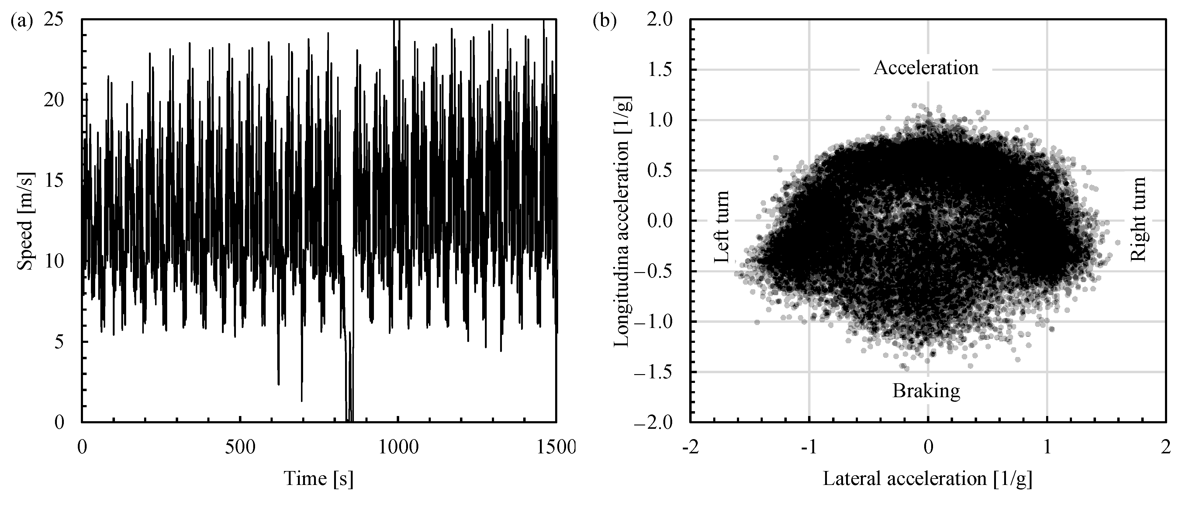
Observing Equation (5), it’s easy to see that the maximum value of vertical force on each front wheel group occurs at maximum deceleration (${\ddot{x}}_G\equiv {\ddot{x}}_{G,min}$). Then, having known the total mass of the vehicle m_tot = 293 kg, along with the wheelbase w = 1535 mm, the distance b = 752 mm, and the height h = 345 mm, telemetric data of a FSAE car was analyzed (see Figure 4) to accurately choose the values of maximum speed and deceleration (to be used in the calculation of kinetic energy, Equation (1)). In particular, Figure 4a shows that the profile of the car’s longitudinal speed during a race has a maximum value $v_{max}=25 \mathrm{m}/\mathrm{s}$. Figure 4b, instead, shows the so-called g-g map, i.e., a map of the vehicle’s longitudinal acceleration versus the lateral one (both normalized to the acceleration of gravity g = 9.81 m/s²). The latter allows us to identify a maximum deceleration of ${\ddot{x}}_{\mathrm{G},min}=-1.5 \mathrm{g}$, which results in $m_{\mathrm{F},max}=121 \mathrm{k}\mathrm{g}$ (~0.4∙m_tot) and $E_{\mathrm{K},\mathrm{F},max}=34.7 \mathrm{k}\mathrm{J}$.

The choice of the right motor size has been made by ensuring it delivers enough power to accelerate the flywheel in the same way as the car accelerates the wheel assembly under real operational conditions. An initial estimate has been made through a straightforward energy balance equation. Essentially, if friction and other forms of energy loss are ignored, the electric motor’s power to accelerate the flywheels from a standstill to their top speed is the following:

$$P_{\mathrm{m}}=\frac{\mathsf{\Delta }{E}_{\mathrm{K}}}{\mathsf{\Delta }t}=\frac{E_{\mathrm{K},max}}{\mathsf{\Delta }t}$$

(6)

where $\mathsf{\Delta }t$ represents the time required to accelerate a stationary car up to 25 m/s. Thanks to Figure 4b, an average longitudinal acceleration of ${\ddot{x}}_{\mathrm{G},max}=+0.6 \mathrm{g}$, which results in $\mathsf{\Delta }t=v_{max}/{\ddot{x}}_{\mathrm{G},max}=4.2 \mathrm{s}$, has been estimated. Once inserted into Equation (6), a motor power requirement of P_m = 9 kW has been found.

The second crucial parameter for selecting the motor is the rotation speed. As shown in Figure 1, the brake assembly is installed on a rotating shaft whose speed is related to the car’s maximum speed by the following relationship:

$${\omega }_{max}=v_{max}/R_e$$

(7)

thanks to which a value of ${\omega }_{max}=106.4 \mathrm{r}\mathrm{a}\mathrm{d}/\mathrm{s}$ (two or three times smaller than the maximum speed of a commercial dynamometer), with $R_e=235 \mathrm{m}\mathrm{m}$ being the front wheel’s effective rolling radius. Accordingly, the bench features a three-phase asynchronous ELVEM T2H-132M4 electric motor with four poles supplied at 380 V, with a nominal power of 9.2 kW and a nominal rotation speed of 1455 rpm, i.e., 152.4 rad/s. Then, the belt drive system connecting the electric motor to the main shaft has been sized to ensure the maximum shaft rotation speed is 105.8 rad/s, with the transmission ratio between the driven and driving pulleys being τ = 125 mm/180 mm = 0.694.

Finally, an estimate of the magnitude of the flywheel mass’s moment of inertia $I^{*}$ to replicate the car’s kinetic energy has been made using the following relationship:

$$E_{\mathrm{K},max}=\frac{1}{2}·I^{*}·{\omega }_{max}^2$$

(8)

from which $I^{*}=2E_{\mathrm{K},max}{\omega }_{max}^2 ~ 6.7 \mathrm{k}\mathrm{g}·{\mathrm{m}}^2$ has been estimated, this value being the same as the smallest of commercial dynamometers and at least tens or even hundreds of times smaller than their average inertia.

The brake system of the bench can be properly sized by knowing two fundamental parameters of the car: the maximum brake torque and brake line pressure. The maximum braking torque has been estimated by referring to the locked brake configuration, i.e., when the tire is the pure longitudinal slip. Referring to Figure 3, the incipient slip of the front tire is obtained when the maximum applied braking torque equals the moment generated by the maximum longitudinal force between the tire and the ground at the contact point F_xF,max:

$$M_{\mathrm{b},max}={\mu }_{\mathrm{x}}·m_{\mathrm{F},max}·g·R_e$$

(9)

where $M_{\mathrm{b},max}$ is the maximum brake torque and ${\mu }_x\approx 1.7$ is the static longitudinal friction coefficient between tires and (dry) asphalt. For the considered test bench, a maximum braking torque $M_{\mathrm{b},max}\approx 500 \mathrm{N}\mathrm{m}$ was obtained, and a slightly higher value (600 Nm) was adopted to size the entire system. Interestingly, the required brake torque is much smaller than that of a commercial dynamometer. A similar conclusion can be drawn with respect to the maximum brake line pressure $p_{max}$ since it ranges from 30 to 50 bar, while it is in the order of 200 bar for commercial dynamometers.

3. Sensors and Control Electronics

The system is equipped with several sensors that allow for precise measurement of the shaft’s rotation speed, the brake line pressure, the disc temperature, the pedal travel, the pedal force, and the braking torque.

Specifically, disc temperature is measured using a Texys INFKL-800 infrared sensor, which is installed on the brake caliper support (Figure 2c), in the same position it has on the FSAE car. Pedal travel is measured using an Aviorace DIA9.5-50 linear potentiometer installed next to the oil pump so as to mimic the exact pedal travel during the braking phase (Figure 2d). The pedal force is measured by means of a custom bending ring-type strain gage load cell (where four strain gauges are bonded to an aluminum ring and connected in a full Wheatstone bridge configuration) that allows to measure tension-compression axial forces up to ±750 N (Figure 2d).

Finally, the most important sensor is that used to measure the braking torque. It consists of a single-axis load cell placed between the brake caliper support and the bench frame (see Figure 5). It must be noted that the brake caliper support is connected to the rotating shaft through two slightly loose ball bearings (Figure 5a), which allow it to rotate and float relative to the shaft. However, the rotary movement of the caliper support is inhibited by the load cell, since it is fixed to the frame with a known offset from the shaft’s axis (95 mm, as shown in Figure 5b). More specifically, the adopted load cell is a bending ring-type strain gage load cell that is designed to work in compression (see Figure 5b) and enables measurement of tension-compression axial forces up to ±7 kN (this value being chosen to read the maximum brake torque, i.e., 600 Nm/0.095 m).

The mechanical system and sensor network are fully interfaced and integrated into an electronic control system based on National Instruments PXI (Figure 2b). Specifically, it consists of a NI PXI-8106 controller with an Intel Core 2 Duo processor running Windows XP as the operating system and is housed in an NI PXI-1052 chassis. Signal generation for bench control and data acquisition is made possible thanks to the NI PXI-6289 M Series multifunction I/O Data Acquisition (DAQ) device, a system equipped with various analog and digital inputs/outputs and two counters. The physical connection of various bench components and sensors to the DAQ is achieved through a dedicated NI SCB-68 terminal block. The system also includes an NI SCXI 1520 module with an SCXI-1314 terminal block, allowing the strain gage to measure the two load cells. The comprehensive management of all sensors and components is enabled by custom LabView code specifically developed for the system.

4. Rotation Speed

Previously, it was noted that the bench has been designed to simulate braking from an initial velocity equal to the vehicle’s maximum speed. Nevertheless, this operational mode does not encompass the full spectrum of testing conditions to which an actual braking system may be subjected. For this reason, the bench is equipped with a commercial three-phase inverter, the ABB ACS355-03E-23A1-4, with a nominal power of 11 kW and an output current of 23.1 A. It allows the variation of the motor’s rotation speed by simply increasing or decreasing the stator field frequency that powers the motor. The power circuit of the inverter consists of a rectifier, which converts the incoming three-phase AC into a DC signal; a bank of capacitors in the intermediate circuit, necessary to stabilize the voltage output from the rectifier; and an actual inverter capable of transforming the DC current from the intermediate circuit into AC at the desired frequency. In particular, the installed inverter allows the user to define a variable motor supply frequency (and thus its rotation speed) different from the nominal one by means of an analog input voltage from 0 V to 10 V proportional to the desired frequency.

The rotation speed of the secondary shaft is then controlled in a closed loop with a speed sensor placed at one end of the shaft (Figure 2d). This device is characterized by a passive digital Hall-effect sensor A3144, fixed to the frame, and by a magnetic tone wheel, attached to the rotating shaft. The tone wheel houses a series of neodymium magnets, evenly spaced around the circumference, which alter the local magnetic field when passing near the Hall effect sensor and switch its logic level from 0 V to 5 V. Eventually, the rotation speed measurement is made possible by connecting the Hall effect sensor to a counter of the PXI-6289 DAQ and by using the appropriate LabView code.

5. Braking System

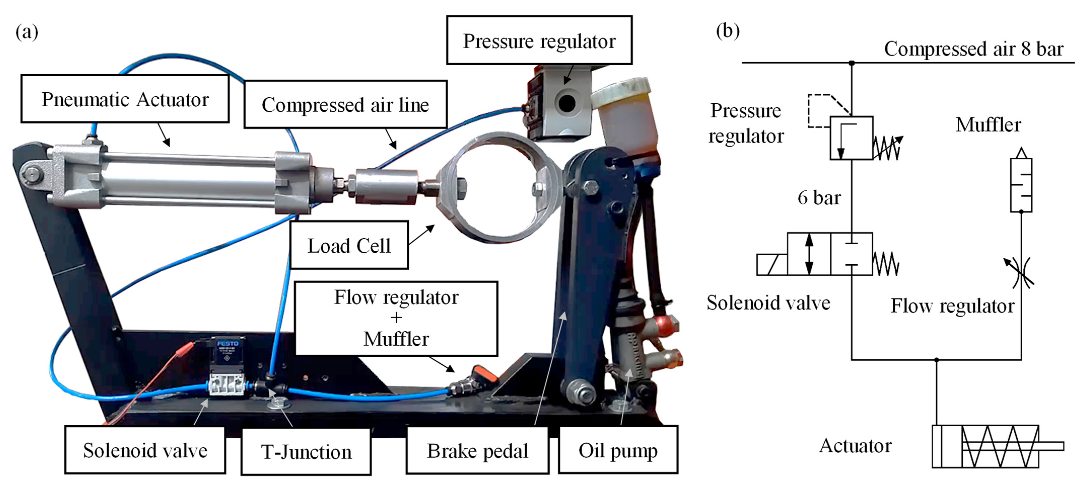
The braking system consists of a brake disc-caliper system that can be easily replaced and adapted to test various types of braking systems, e.g., different brake caliper or pad compounds. The braking force is generated by a dedicated pedal assembly that has been designed to simulate braking conditions similar to those of a Formula SAE car (Figure 6): the brake line is supplied by an AP Racing CP7855 brake pump (bore 14 mm), mounted through rod-ends on a pedal assembly that simulates the vehicle’s kinematics (Figure 6a). The pedal is moved by a pneumatic circuit (Figure 6b) that powers a CAMOZZI 60M1L040A0075 single-acting pneumatic actuator (bore 40 mm, stroke 75 mm). The actuator is equipped with an internal spring located in front of the piston, ensuring its return to the neutral position by simply venting the air inside the cylinder into the atmosphere after the braking phase is completed. Like the brake pump, two hinges are used to connect the actuator to the frame, allowing for purely axial loading. The maximum compressed air supply pressure is set to 6 bar; this value is maintained constant by a pressure regulator valve located immediately downstream of the connection to the supply line (Figure 6).

The air exiting the pressure regulator passes through a normally closed, monostable 2/2 solenoid valve with pneumatic return and electronic activation (FESTO MHJ9-QS-4-MF). Downstream from the solenoid valve, there is a ‘T’ junction: one outlet of the junction directs air to the pneumatic piston, while the other outlet is connected to a ball valve acting as a flow regulator, downstream of which a muffler is mounted to vent the pressurized air into the atmosphere. The flow regulator induces a significant pressure drop; therefore, upon opening the solenoid valve, most of the air will flow into the pneumatic cylinder, with only a portion venting directly into the atmosphere. By adjusting the flow regulator’s opening, the maximum pressure achievable inside the cylinder is regulated. In the current configuration, the flow regulator has been set so as to reach a maximum pressure within the braking circuit of approximately 60 bar.

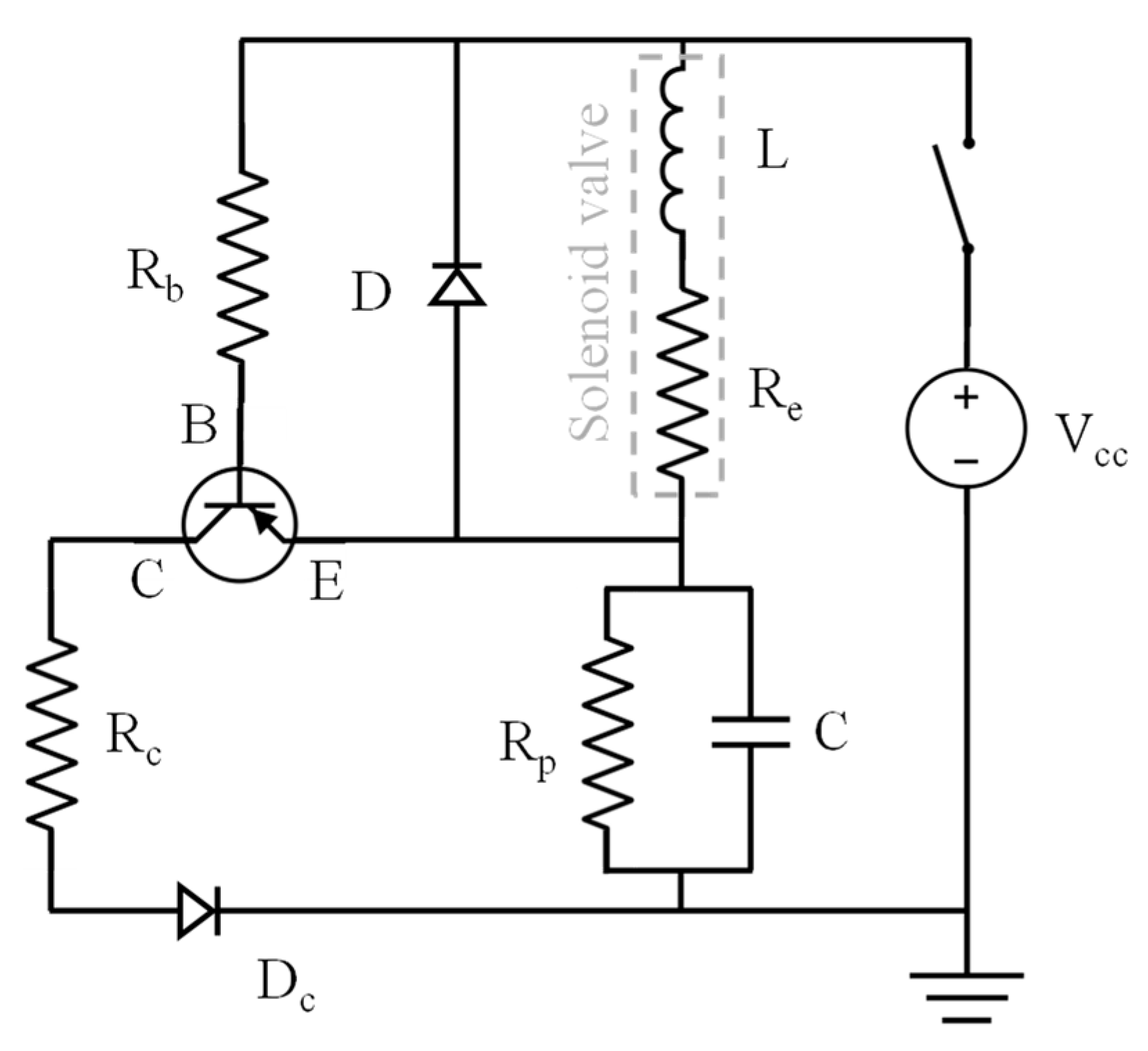
The solenoid valves require a variable current over time to properly operate. Specifically, they open only after a current spike of at least 1.6–1.8 A lasting about 0.5 ms. Once opened, a much lower current value (~0.4 A) is sufficient to keep the solenoid valve open, reducing power consumption and limiting Joule heating to acceptable levels during operation. The circuit enabling this mode of powering the solenoid valve is schematically represented in Figure 7.

The electrovalve, represented as the series of an inductor (L) and a resistor (R_e = 4 Ω), is connected in series with the parallel of a resistor (R_p = 54 Ω) and a capacitor (C = 1000 µF) (see Figure 7). The circuit’s terminals are then connected to a DC voltage generator (V_cc = 24 V) and a main switch that allows to supply or not the solenoid valve circuit. To better understand how it works, consider two different instants of time: in the first one, the circuit is initially open with both the inductor and capacitor discharged and then is closed and supplied at V_cc. Otherwise, the second instant corresponds to the steady-state condition, where the circuit is supplied at V_cc and both the inductor and capacitor are fully charged.

In the first case, the capacitor acts as a short circuit, allowing for a high initial current flow through the electrovalve, its magnitude being approximately I_peak = V_cc/R_e = 6 A. This high current value equals the peak current required to open the solenoid valve. Noteworthily, the description here discussed is a simplified representation of the actual circuit behavior, which includes additional non-linearity related to the inductor’s charge, not considered here. A moment later, the capacitor starts to charge, causing a parallel current (initially zero) through resistor R_p. In the steady state, the charged capacitor acts as an open switch, and the inductor acts as a short circuit. Therefore, the system simplifies to the series of two resistors R_e + R_p = 58 Ω supplied with a current I = V_cc/(R_e + R_p) = 0.41 A. This current value, lower than the previous one due to increased circuit resistance, keeps the electrovalve open, dissipating less power and generating less heat.

Another crucial feature of the circuit is the presence of a freewheel diode (also known as a flyback diode and denoted as D in Figure 7). This diode is connected across the inductor to eliminate flyback, which is a sudden spike voltage observed across an inductive load when its supply current is abruptly interrupted. This diode also minimizes the circuit discharge times (with a time constant ${\tau }_L={L/R}_e$) and, consequently, the switching times of the electrovalve (it opens and closes faster). Then, the other components of the circuit in Figure 7 are necessary to prevent the capacitor discharge phase (${\tau }_C=R_p·C$) from slowing down the system. This includes a PNP transistor TIP34C whose base is connected to the +V_cc supply, the emitter to the positive terminal of the capacitor, and the collector to the negative one. When the whole circuit is powered, the base-emitter junction is reverse-biased, and the transistor is turned off. Conversely, when the circuit is open, the transistor is turned on, and a current flow is allowed between the emitter and collector. This creates a circuit where the capacitor (charged) powers two resistors in parallel (R_p and R_c). However, since R_c = 2.5 Ω << R_p = 54 Ω, the overall resistance of the circuit is R_tot ~ R_c = 2.5 Ω, so the new time constant of the capacitor discharge circuit can be roughly estimated as ${\tau }_c^{\prime }=R_c·C\ll R_p·C$, allowing for a much faster discharge of the circuit and, therefore, a higher switching frequency for the electrovalve.

Now that the power section of the circuit has been clarified, it is worth noting that the main switch of the system, which allows for interrupting the connection of the circuit to the 24 V power supply, is accomplished through a digital-type switch generated by the main controller. Specifically, the control signal generated by the controller comes to the power electrical circuit through a photo-coupler TPL523, a small device that enables communication between two electrical systems while electrically isolating them thanks to a light signal generated by an emitting diode and detected by a receiving diode. Once suitably conditioned and amplified, this signal allows the system to work correctly and prevents potential overcurrent and overvoltage in the power circuit from damaging the controller.

Finally, to continuously vary the compressed air flow into the cylinder, the electrovalve’s opening is modulated with a PWM (pulse width modulation) signal, i.e., by means of a square wave having a set frequency (50 Hz) and variable duty cycle. In the “high” logic state, the electrovalve is powered with the maximum supply voltage (V_cc = 24 V) and fully opens, while in the “low” logic state, it is not powered and remains closed, blocking the flow of compressed air to the actuator.

The control signal is generated through the second digital counter of the DAQ PXI-6289 and is managed by the NI controller with the appropriate LabView code. In particular, the system is controlled by a PID controller that automatically adjusts the duty cycle to maintain the desired braking force. The closed-loop control is based on the signal from a piezoelectric membrane oil pressure transducer (Aviorace SP100-M10 × 1) located on the brake line (see Figure 2c).

6. Testing

6.1. Operating Modes

The test bench offers various testing modes through different possible test protocols:

• Manual. This program allows the operator to choose and vary the rotation speed and brake system pressure in real-time within the allowable maximum values (0–90 km/h, 0–60 bar).
• Constant Speed and Pressure Tests. The system can maintain a constant rotation speed of the shaft and brake system pressure (in this case, the installed motor power, i.e., 9.2 kW, which sets upper limits on usable pressure and speed).
• Brake Ramps at Constant Speed and Set Pressure. In this case, the motor accelerates the brake disc to reach a predetermined target speed within a set time, which is maintained for a certain duration before turning off the motor and starting a braking phase at constant pressure. After the braking phase, it waits for a preset time interval and repeats the same experiment for a number of cycles chosen by the operator.
• Track Data Reproduction. This method allows the motor to simulate inertia and the bench to reproduce any operational condition, particularly those recorded by telemetry from a Formula SAE (FSAE) car during races.

6.2. Speed Profile

Focusing on the last-mentioned operating mode, i.e., that one allowing to replicate on-track conditions on the test bench, the operator inputs to the controller a .csv file containing 4 columns of data corresponding to time (in seconds), oil pressure (in bar), brake disc temperature (in °C), and vehicle speed (in km/h). Then, the system reads the .csv file and automatically replicates the entered speed, oil pressure, and disc temperature profiles. However, given the input speed profile, the actual profile replicated at the bench is a function of the installed flywheel mass. In more detail, the maximum inertia of the bench has been sized with respect to the most severe braking conditions, which never happened during a race. For the same braking force, excessive flywheel inertia results in lower deceleration compared to the input one (and vice versa, since if the flywheel inertia is too small, the motor has not enough power to replicate the wanted speed profile). In other words, there exists an optimum value of the flywheel inertia that allows for the proper reproduction of the input speed profile on the test bench.

To find its value, preliminary tests can be performed by discretely varying the flywheel mass, i.e., by removing one flywheel at a time between runs, and by comparing the speed profile obtained for each configuration. The optimal number of flywheels is the one that minimizes the difference between the input speed profile and that of the bench. An example is shown in Figure 8, where the input speed and pressure profiles are depicted in black and red, respectively. The same figure shows the same quantities as replicated by the test bench. In particular, the grey line represents the pressure profile generated by the brake pedal assembly, while the other colored lines represent the bench’s speed profiles with a different number of flywheels. Specifically, a total of 6 flywheels (five of type A and one of type B having polar moments of inertia equal to 1.401 kg∙m² and 0.272 kg∙m², respectively) have been used in different combinations. In the specific case considered, the optimal one consists of two type A flywheels and one flywheel of type B, the difference between the input speed profile and the applied one being minimized during deceleration phases (compare the black and purple lines in Figure 8). The same figure shows that a different total number of flywheels obviously results in a higher difference between input and measured speed profiles (compare the orange, yellow, green, and blue lines with the black one in Figure 8), with the deceleration being less than the desired one the greater the number of flywheels, and vice versa.

6.3. Cooling System

Another key aspect of the test bench is the cooling system, which can be turned off, run continuously at maximum flow, or operated variably to ensure faithful reproduction of a temperature profile given as an input to the main controller. In more detail, the cooling system mimics the vehicle’s cooling conditions and consists of a SAN ACE 140 L-9LG1424P5G001 fan that directs airflow directly onto the brake disc and caliper, as illustrated in Figure 9.

It is well known that temperature is a parameter that has a huge influence on the brake system performance [7,22,30,32], so the need for implementing a cooling system becomes evident when observing the difference between the red temperature profile and the black one in Figure 10. It is noticeable that the temperature profile reproduced on the bench without the fan (no fan—red line in Figure 10) differs significantly from the one originating on the track (black line in Figure 10), showing differences of up to approximately 120/130 °C. Noteworthily, as observed in [7,22,32], the effect of cooling air direction relative to the brake and its distance from the rotor has a relatively low influence on the test results, suggesting the possibility of positioning the cooling system without the need to faithfully replicate the operational conditions of the car, where the airflows can assume complex and difficult-to-reproduce patterns.

Accordingly, the selection of the ventilation system was made through various experimental tests, which not only helped to choose the proper fan but also identified that variations of the airflow incidence within 0° and 45° relative to the disc have a limited influence on the thermal exchange, although its magnitude is slightly higher when positioning the fan at 45°. The same preliminary tests also confirmed that running the fan at a constant maximum speed during the test could result in excessive heat removal, causing the system to be overcooled compared to the required temperature profile.

For this reason, the cooling system is supplied with variable voltage to modulate the fan’s rotation speed (ranging from 2300 to 7500 rpm) and, consequently, adjust the airflow. To achieve this, the fan is powered by a continuous voltage of variable magnitude generated using a PWM signal. Modulation is made possible through closed-loop control based on the input temperature profile, which automatically increases the rotation speed when the temperature difference between the bench and the target value is detected and decreases it in the opposite case. In this way, the bench can accurately track the target temperature profile, with their difference being maintained within ±15 °C, as shown in Figure 10.

7. Conclusions

This study presented the design and development of a brake test bench tailored for Formula SAE (FSAE) race cars. The bench incorporates a rotating shaft system, pneumatic brake pedal simulation, and an array of sensors to evaluate various brake disc-caliper combinations and pad materials. The system’s design enables the measurement of critical parameters such as rotation speed, braking torque, oil pressure, and disk temperature, providing a comprehensive overview of brake performance under different conditions. The research detailed the bench’s structure, the selection and integration of sensors, and the control electronics, highlighting its capability to simulate on-track braking scenarios in a controlled environment. The findings demonstrate the bench’s utility in offering precise and repeatable testing conditions, which are crucial for analyzing the efficiency, durability, and safety of braking systems in FSAE race cars. While the paper primarily focuses on the bench’s conceptualization, construction, and initial testing, the results lay a solid groundwork for subsequent, more in-depth studies and optimizations of FSAE braking systems. The approach and methodologies employed offer a valuable reference for similar future endeavors aiming at enhancing performance and safety in automotive engineering.