Analysis of Roughness, the Material Removal Rate, and the Acoustic Emission Signal Obtained in Flat Grinding Processes

Abstract

In this work, the analysis of the acoustic emission (AE) signal in grinding processes is addressed. The proposed analysis method decomposes the acoustic signal into three frequency ranges. The total energy of each range is determined, as well as the highest frequency. Different grinding experiments were carried out, according to a full factorial design of experiments (DOE), in which feed speed, depth of cut, and transversal step (table cross feed) were varied. Arithmetic average roughness Ra and the material removal rate (MRR) were determined. It was observed that Ra depends mainly on the transversal step, followed by feed speed and the interaction between the transversal step and depth of cut, while MRR is greatly influenced by the transversal step. According to multi-objective optimization with the Derringer–Suich function, in order to simultaneously minimize Ra and maximize MRR, a transversal step of 9 mm per longitudinal pass, feed speed of 20 m/min, and depth of cut of 0.020 mm should be selected.

1. Introduction

Surface grinding is an abrasive machining process for flat surfaces. Specifically, in traverse grinding, a grinding wheel turns while the table where the workpiece is placed combines transversal and longitudinal movement, provided by feed speed (in a reciprocating movement) and the cross-feed or transversal step, respectively [1,2]. Two main differences between abrasive machining processes and cutting processes are that in abrasive machining processes, much smaller chips are produced, and a higher amount of energy is required in abrasive machining processes to remove the same material volume. This is mainly attributed to negative rake angles and rubbing and plowing between the wheel and the workpiece [2]. In addition, the cutting-edge geometry in abrasive machining processes is stochastic rather than deterministic.

Machining processes provide different acoustic emission (AE) signals depending on the used process parameters. Nowadays, the use of AE signal analysis for the analysis of machining processes is increasing. Based on the obtained sound signal, it is possible to non-invasively supervise the machining process, i.e., it is possible to control it without interrupting the operation of the machine tool. For example, the condition of the machine and the degree of tool wear can be checked. Adeniji et al. [3] developed a real-time and non-destructive evaluation quality technique for the monitoring of conducted machining processes based on AE signals, wavelet transform, and deep neural networks. They integrated an AE sensor into the cutting tool holder to maintain constant signal attenuation during cutting. Barylski and Sender [4] paid extensive attention to the possibility of creating automated numerically controlled machines which, in addition to other sensors, contain acoustic sensors and computational algorithms used to supervise machining processes. Fernando Chacón et al. [5] stated that tool wear is a critical aspect that requires real-time monitoring, for instance, using AE analysis, to reduce costs and the scrap received in machining processes. Rimpault et al. [6] concluded that cutting forces and AE signals depend strongly on tool wear. They used fractal analysis and found variations in tool wear. Gómez et al. [7] studied a drilling process with different degrees of tool wear and found relationships between acoustic emission (AE) and torque. Kuntoglu et al. [8] stated that indirect tool condition monitoring systems can use sensors situated around the cutting area to check the wear condition of a cutting tool without intervention in the cutting zone. Murat et al. [9] confirmed the high precision of the analysis method using AE signals for drill wear level classification from sharp to completely worn drill. Nahornyi et al. [10] proposed using the generated sound during machining as the operational information needed for the adaptive control of the metalworking process and also for early monitoring and diagnosis of the condition of the machined materials. Sio-Sever et al. [11] presented a prototype of a system for estimating the milling parameters from an AE signal using AI procedures. Zhang et al. [12] studied a new deep learning model to identify tool wear. The force signal was transformed into a two-dimensional image using continuous wavelet transform and short-time Fourier transform. The generated images were then fed into a convolutional neural network (CNN) model for further analysis. The accuracy of the proposed tool wear state recognition method was above 90%. Ho et al. [13] defined a new direction for the monitoring of the machining process using machine learning tools to analyze recorded data during machining, such as cutting force, acceleration, sound, image, etc.

Researchers are also involved in the analysis of the influence of machining parameters on the vibrations obtained. For example, Huda [14] detected chatter in turning processes by analyzing AE. Nikhare et al. [15] stated that, over time, a cutting tool reaches its end-of-life, which increases the cutting force and thus produces more vibration and noise. Nourizadeh et al. [16] described that the sound generated by tool holder vibration will result in a low-frequency sound, while the sound generated by the friction mechanism is a high-frequency signal. They also described that the sound generated by metal deformation produces a mid-range frequency signal. They also showed that the main portion of the energy in a machining process is consumed for metal deformation. Papacharalampopoulos et al. [17] stated that there are several mechanisms for the inspection of tool wear, especially using the AE method. The obtained signals can be affected by tool geometry, machine vibrations, and noise. Perrelli et al. [18] proposed two algorithms for chatter detection, from the calculation of two chatter indicators, based on Power Spectral Density and Wavelet Packet Decomposition analysis of the monitored signals.

As for the operation of abrasive machining processes, Chen and Wang [19] observed that bivariate empirical mode decomposition (BEMD) and Hilbert transform are reliable methods for processing simulated and experimental chatter signals obtained during the CNC grinding process because of good behavior in terms of processing nonstationary and nonlinear signals. Leaman [20] observed that using empirical mode decomposition (EMD) is a complementary signal processing technique in gearbox analysis. Amarnath and Praveen Krishna [21] stated that EMD extracted from sound signals provides good diagnostic information due to its ability to decompose signals into high- and low-frequency modes. Deja [22] showed that utilizing microphones as audible sound sensors is a suitable approach for monitoring a single-side lap grinding process. Sender and Buj-Corral [23] reported that the AE signal analysis can be used to assess the correct operation of abrasive stones in honing processes. Liao [24] monitored the grinding wheel condition using AE signals, which were extracted with discrete wavelet decomposition and autoregressive models.

Regarding the surface finish, Pilny et al. [25] described the surface roughness obtained in the polishing process and found a correlation between decreasing AE amplitude and surface roughness Ra. Mirifar et al. [26] studied the connection between AE signals and grinding outputs, e.g., surface roughness and grinding forces, using neural networks. Nguyen et al. [27] proposed a prediction technique for surface roughness in grinding processes by decomposing the original AE signals into intrinsic mode functions (IMFs) with the empirical mode decomposition (EMD) method. Hatami et al. [28], using a corundum wheel of grit 46, checked that the lowest average surface roughness value (0.70 μm) was obtained using a feed rate of 100 mm/s (6 m/min), while the highest value (0.87 μm) was obtained using a feed rate of 300 mm/s (18 m/min). Demir et al. [29] confirmed that, when using depth of cut of 0.04 mm and 0.05 mm, the Ra obtained with an 80-grain wheel was better by 30, 80, and 400% than those for 60, 46, and 36-grain wheels. Wang et al. [30] showed that surface roughness tended to increase gradually with the increase in cutting depth and workpiece feed speed. Wen et al. [31] found that, as grinding depth decreases, the grinding force of coated micro-grinding tools is continuously reduced, which decreases the impact of the tools on the surface of a specimen; and the surface roughness of the specimen is thus reduced. Ying et al. [32] stated that, when the grinding depth increased from 0.01 mm to 0.05 mm, the surface roughness profile parameter Ra increased from 0.13 µm to 0.19 µm, because the contact time between abrasive particles and samples prolongs as the grinding depth increases. They also stated that the number of abrasive particles that participate in grinding in the grinding area increases, thus increasing the overall grinding force. This makes particles easier to pull out [33]. However, some authors report a decrease in roughness with feed speed, for example, Ruzzi et al. [34] as well as Ma et al. [35], who also found a decrease in roughness with depth of cut. As for the transversal step or table cross-feed, Patel et al. [36] found that it has an important effect on roughness, when grinding EN8 steel with alumina of grit size 60.

Concerning the material removal rate (MRR), high values up to 80 mm³/mm·s were reported by König and von Arciszewski [37] for high depth of cut values up to 8 mm. Thus, the material removal rate is known to increase with depth of cut. Kumar et al. [38] stated that the optimal combination of parameters is a wheel speed of 850 min⁻¹, a table speed of 15 m/min, and a depth of cut of 11.94 µm in order to achieve a maximum MRR and minimum surface roughness. Walton et al. [39] stated that high specific material removal rates (SRR) of 1000 mm³/mm²·s produce thermal damage on workpieces’ surfaces, with severe re-hardening burn. Ma et al. [40] reported that the MRR is influenced by many parameters such as wheel speed, feed speed, dressing, wheel surface, workpiece surface, etc. For the surface grinding of AISI D3 steel, Singh et al. [41] found that depth of cut was the main parameter influencing the MRR.

Regarding the energy of the AE signal, Kwak and Ha [33] found that both the peak value of RMS and the peak value of FFT increased with feed speed in grinding processes. Yin et al. [42] investigated the relationship between processing parameters and characteristic parameters of the AE signal including the RMS value, ringing count, and signal spectrum during grinding. They found that the RMS value of the AE signal increased with grinding depth and feed velocity and decreased with an increase in grinding wheel linear velocity when grinding GH4169 superalloy, TC4 titanium alloy, and SiCp/Al composite. Webster et al. [43] observed that in grinding processes, the normal force/AE ratio had a good correlation with surface roughness.

In this work, the effect of three flat grinding parameters (feed speed, transversal step, and depth of cut) on surface roughness and the material removal rate is addressed using a full factorial design of experiments. Using multi-objective optimization, appropriate values of the grinding parameters are searched for in order to simultaneously minimize roughness and maximize the material removal rate. In addition, the acoustic emission (AE) signal is measured for the different experiments. Each signal is divided into three groups of signals, and the maximum frequency is determined for each group. Sound signal energy parameters Ey1, Ey2, and Ey3 are also calculated. The maximum frequency values for each group conform to a specific pattern for this process. In cases where there was a problem in the grinding process, the pattern would change, thus allowing us to monitor the process.

2. Materials and Methods

2.1. Materials

Carbon steel blocks made from St-52 steel of dimensions 50 × 50 × 200 were machined in a Perfect tangential grinding machine, with a corundum abrasive wheel of grain size 60 (Norton scale). The cutting speed was 30 m/s in all experiments.

2.2. Grinding Experiments

This research consisted of grinding experiments on a flat surface, in which the depth of cut, feed speed, and transversal step, also known as cross feed, were varied. The acoustic emission (AE) signal was recorded. In addition, the average surface roughness Ra and material removal rate (MRR) were determined in all experiments.

In the grinding tests, a three-factor two-level full factorial 2³ design plan was used, with 3 central points, which summarizes 11 layouts. The full factorial design can be visualized as a cube with an experimental run at each of the cube’s corners. A regression analysis of the 2³ full factorial experiments can fit the following model (1):

$$\mathrm{y}={\mathrm{b}}_0+{\mathrm{b}}_1{\mathrm{x}}_1+{\mathrm{b}}_2{\mathrm{x}}_2+{\mathrm{b}}_3{\mathrm{x}}_3+{\mathrm{b}}_{12}{\mathrm{x}}_{12}+{{\mathrm{b}}_{13}{\mathrm{x}}_{13}+\mathrm{b}}_{23}{\mathrm{x}}_{23}+{\mathrm{b}}_{123}{\mathrm{x}}_{123}$$

(1)

where the bs are all regression coefficients.

The b₀ term is referred to as the model’s constant. The coefficients b₁, b₂, and b₃ are called the main effects and the b₁₂, b₁₃, and b₂₃ terms are two-factor interactions. The coefficient b₁₂₃ is established as a three-factor interaction.

The grinding experiments are shown in

Table 1. Parameters: transversal step (mm), feed speed (m/min), depth of cut (mm); responses: average roughness—Ra, material removal rate—MRR.

Run Order	Transversal Step (mm)	Feed Speed (m/min)	Depth of Cut (mm)	Ra (µm)	MRR (mm/min)
1	3	12	0.010	0.447	0.0178
2	9	12	0.010	0.554	0.0310
3	3	20	0.010	0.395	0.0231
4	9	20	0.010	0.442	0.0308
5	3	12	0.020	0.378	0.0202
6	9	12	0.020	0.601	0.0307
7	3	20	0.020	0.350	0.0211
8	9	20	0.020	0.536	0.0300
$\overline{9}$	6	16	0.015	0.456	0.0242

, together with the Ra and MRR results. Experiment 9 corresponds to the center point of the design, in which all the variables are kept at their middle values, i.e., depth of cut of 0.015 mm, feed speed of 16 m/min, and transversal step of 6 mm per longitudinal pass. Experiment 9 was repeated three times. The average value for this experiment is presented in Table 1.

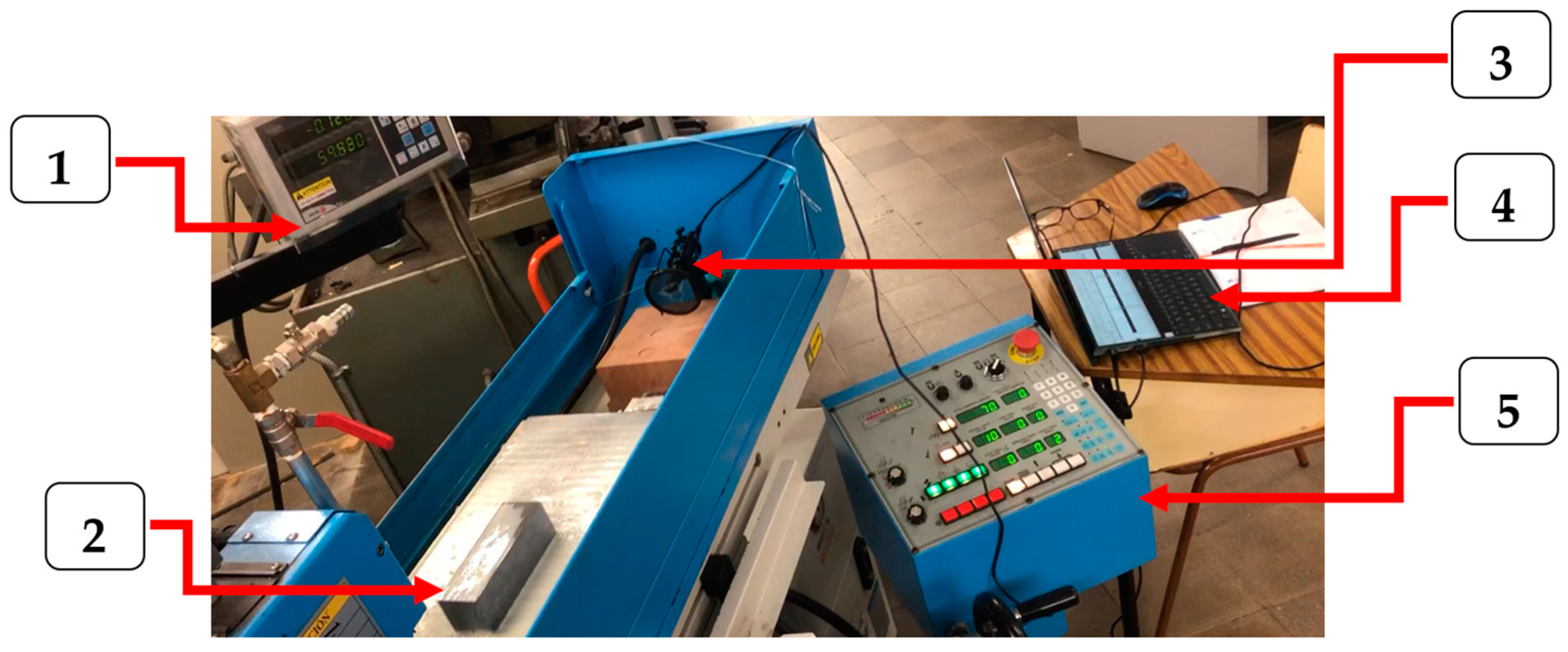
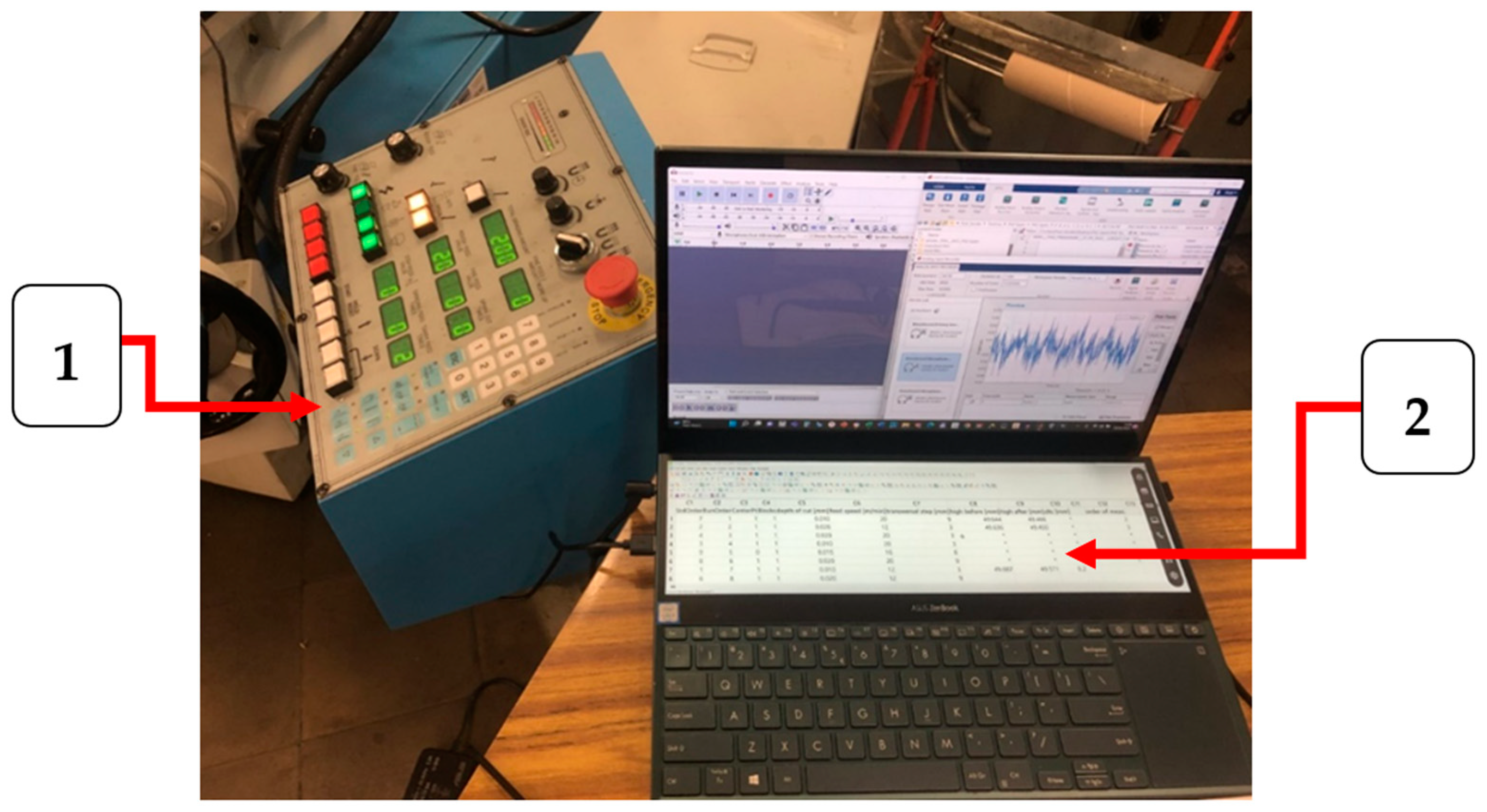
2.3. Experimental Setup

Figure 1 shows the tangential grinding machine made by Perfect Machine Co., Ltd., (Taichung, Taiwan), model PFG-2550AH, which was used in the experimental tests. This research was conducted at the Manufacturing Technologies Laboratory of the Barcelona School of Industrial Engineering (ETSEIB), Universitat Politècnica de Catalunya in Spain.

A directional condenser microphone made by Trust company (Dordrecht, The Netherlands) model Velica, was mounted in the machining area of the grinding machine (Figure 2) and used for recording of AE signal. The advantage of directional microphones is that they record acoustic signals mainly from the direction in which a microphone is placed, which largely eliminates most acoustic signals that could be recorded from the surroundings.

The selected responses are the energy of the AE signal (Ey1, Ey2, and Ey3), average roughness Ra, and the material removal rate, MRR (see Section 2.4, Section 2.5 and Section 2.6).

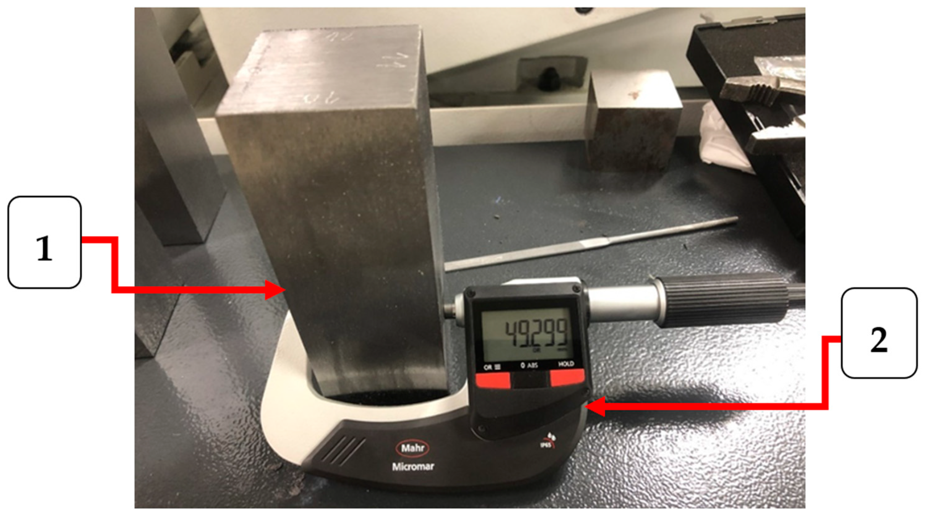
2.4. Roughness Measurements

Roughness was measured with a Taylor Hobson (Leicester, UK) Talysurf 2 contact roughness meter. A Gaussian filter was used with a cut-off length of 0.8 mm. The measurement length was 4.8 mm. The arithmetic average roughness parameter Ra was considered.

2.5. Determination of the Material Removal Rate (MRR)

In order to determine the material removal rate, the height of the blocks before and after the grinding operation was measured with a Mahr digital micrometer (Figure 3).

In this work, MRR (mm/min) was considered as the height reduction in the blocks per time unit.

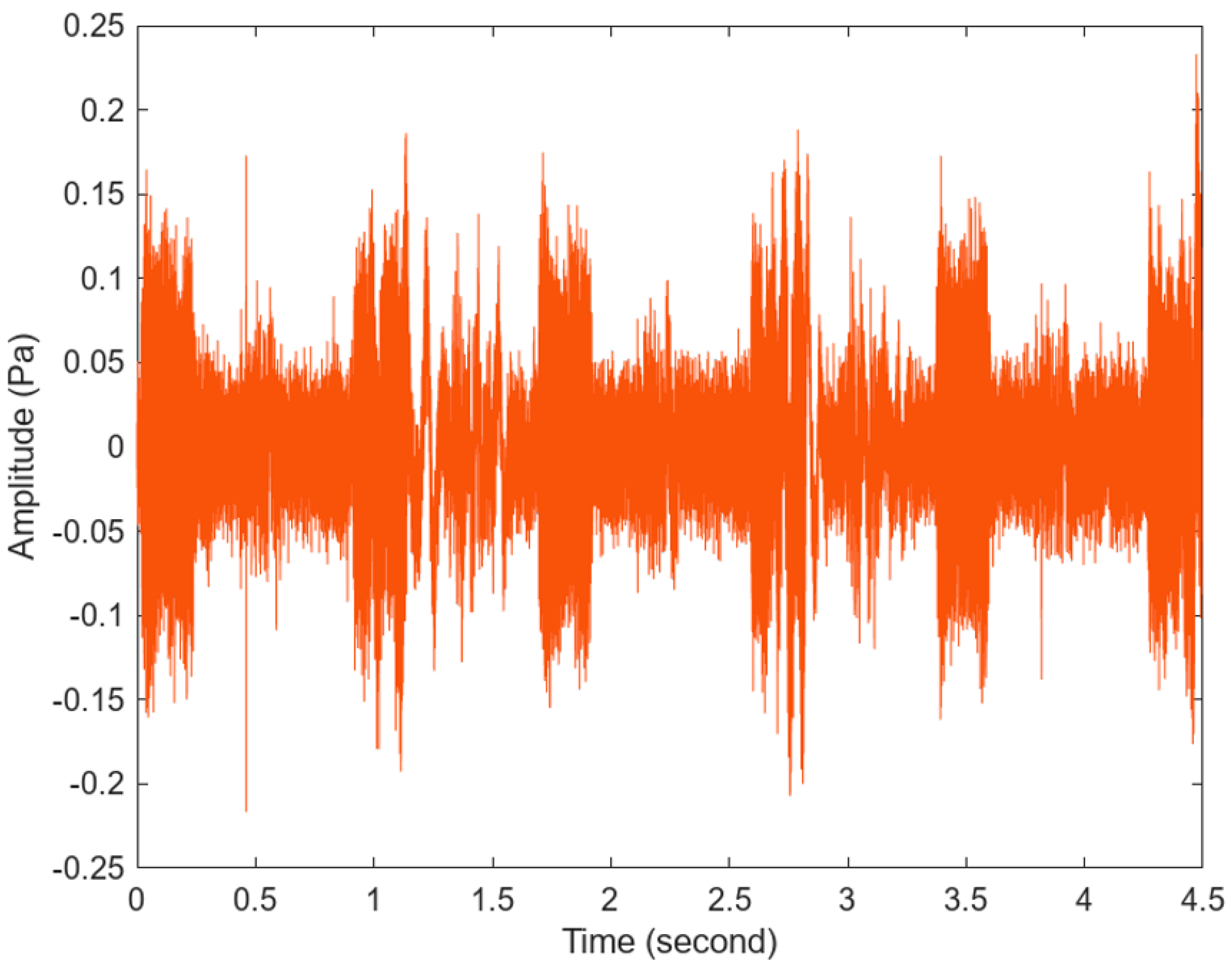
2.6. Measurement of the AE Signal

The AE signal was recorded with a microphone (see Section 2.3). Figure 4 shows a laptop with Audacity and Matlab software installed. The laptop is connected to the directional Trust’s microphone.

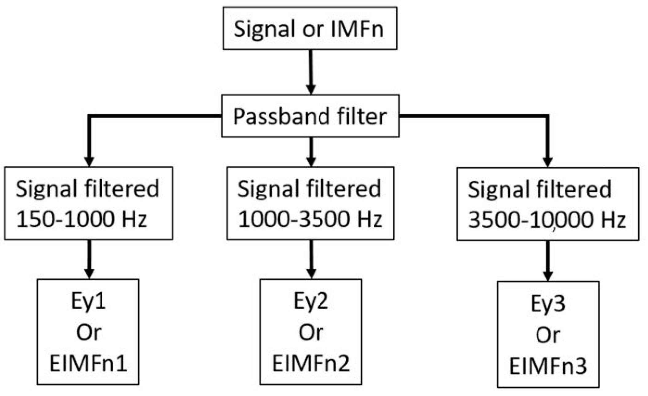
2.7. Analysis of the AE Signal

The proposed analysis method used to decompose the acoustic emission (AE) signal into three frequency ranges is as follows (Figure 5):

-

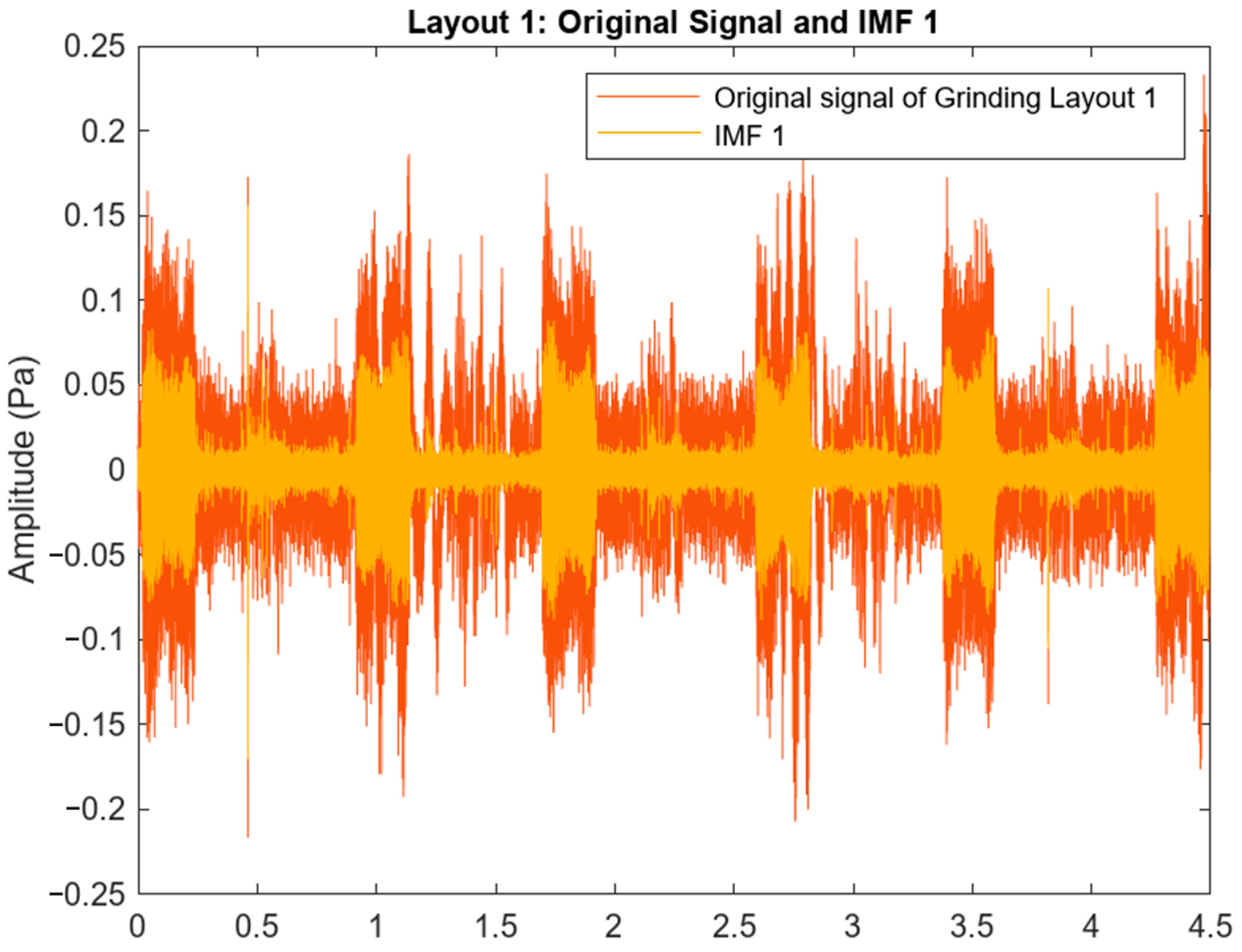
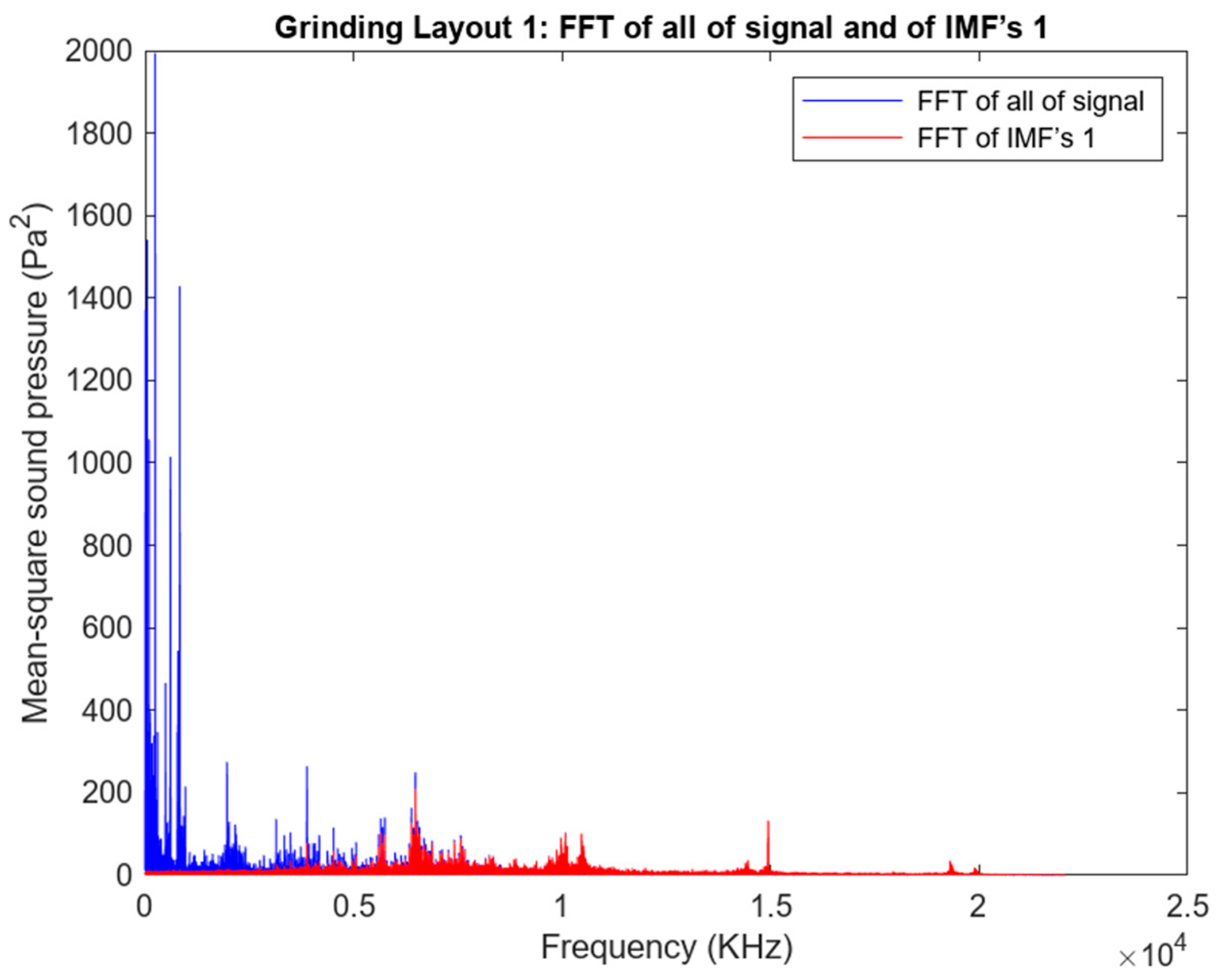
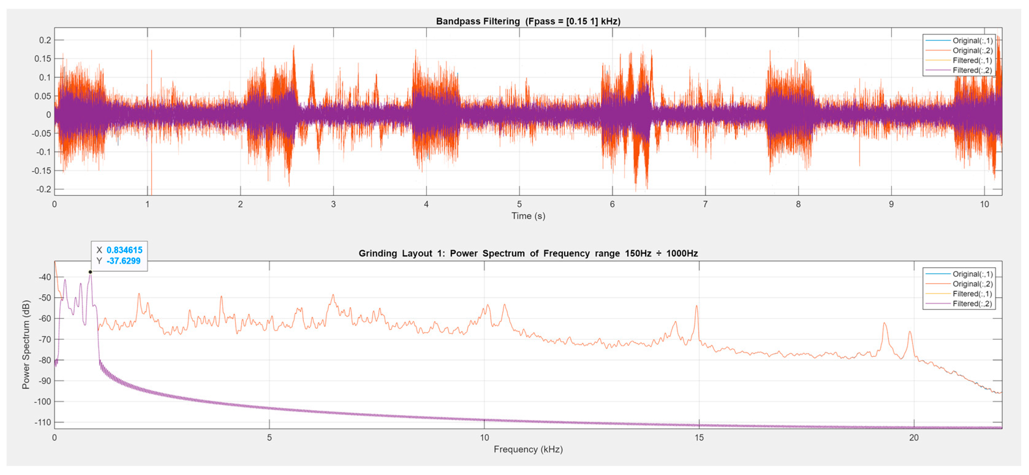
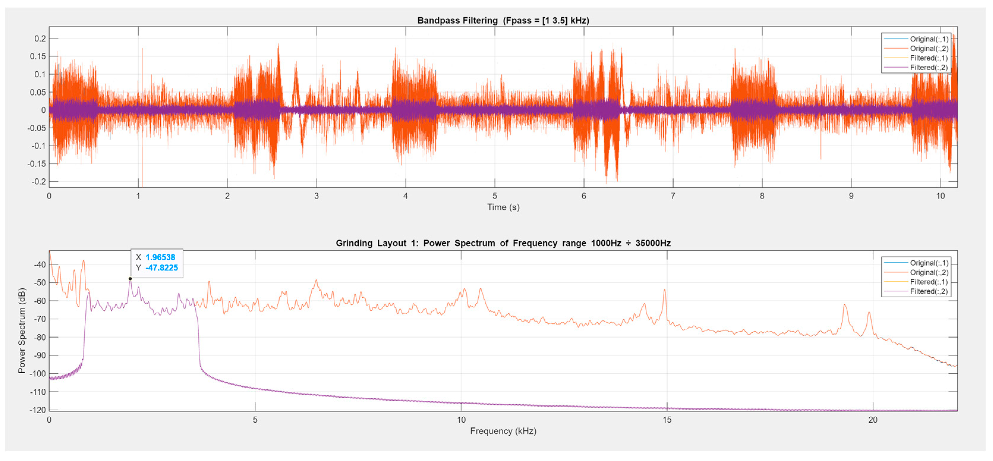
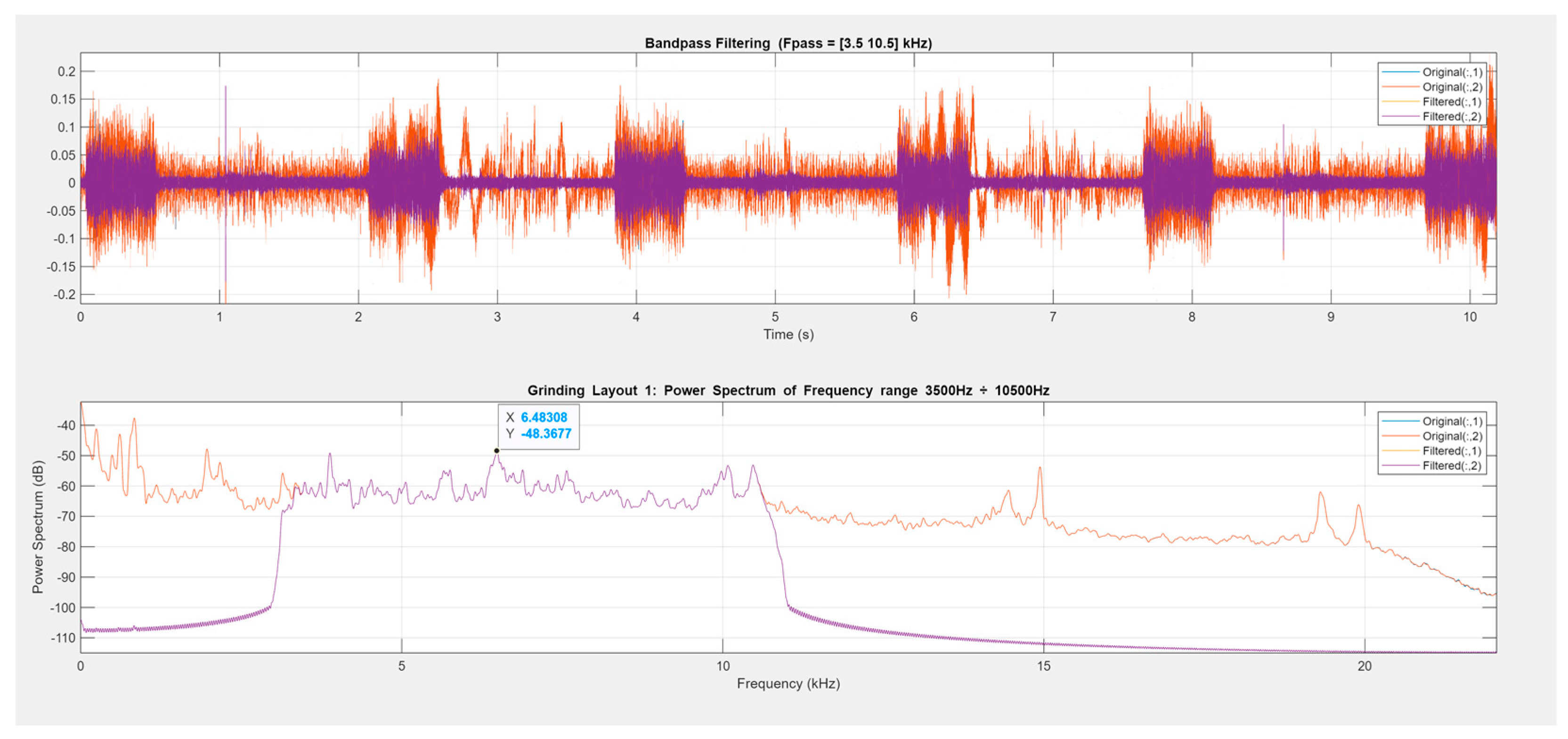
First, the frequency bands are established. The signal is decomposed into three different signals, using band pass filters. In this case, the selected frequency ranges were as follows: for the first band, 150 to 1000 Hz; for the second band, 1000 to 3500 Hz; and for the third band, 3500 to 10,000 Hz. Other values can be established depending on the type of machining or machining conditions. Alternatively, IMFs can be used instead of the signal. They are obtained with the empirical mode decomposition (EMD) method.

-

The next step is to measure the power spectrum for the different frequency ranges of the analyzed AE signals.

-

In addition, X is calculated as the frequency of the highest peak of the filtered signal (in kHz), while Y is the power spectrum in dB.

3. Results and Discussion

3.1. The Material Removal Rate and Surface Roughness

Table 1 summarizes the experiments that were performed, as well as the results of the grinding tests.

The highest Ra value of 0.601 µm corresponds to experiment 6, with a high depth of cut of 0.020 mm, low feed speed of 12 m/min, and high transversal step of 9 mm per longitudinal pass. The lowest Ra value of 0.350 µm was found in experiment 7, with a high depth of cut of 0020 mm, high feed speed of 20 m/min, and low transversal step of 3 mm per longitudinal pass. This suggests that, within the ranges studied, not only the feed speed but also transversal step, also known as cross feed, have an important influence on surface roughness. This was also reported by Patel et al. [36]. Similar roughness values were obtained by Hatami et al. [28] with a grinding wheel of grit size 46. According to Demir et al. [29], the higher cutting depth and feed speed, the greater the number of effective dynamic grinding edges and the maximum undeformed chip thickness, thus enhancing the depth of the grinding marks, the grinding force, and the grinding heat. As a result, the roughness parameter Ra increases. In this work, roughness increases with depth of cut when a high transversal step is considered (experiments 2 and 6 or experiments 4 and 8). However, when a low transversal step is used, the opposite behavior is observed (experiments 1 and 3 or experiments 5 and 7). This reduction in roughness with depth of cut was also reported by Ma et al. [35] for glass–ceramics. On the other hand, in this work, Ra tends to decrease with feed. This effect was previously reported by Ruzzi et al. [34] when grinding Inconel. On the other hand, the higher the transversal step, the lower the overlap between consecutive passes, leading to higher roughness [36]. This phenomenon is found in the present work, for example, when comparing experiments 1 and 2, 3 and 4, 5 and 6, or 7 and 8.

The highest MRR values around 0.0300 mm/min were obtained in experiments 2, 4, 6, and 8, with a high transversal step of 9 mm per longitudinal pass. The lowest MRR value was reported in experiment 1, with a low depth of cut of 0.010 mm, low feed speed of 12 m/min, and low transversal step of 3 mm per longitudinal pass. Thus, within the studied range, the transversal step has an important influence on the MRR. Similar depth of cut values of 0.012 mm and feed speed values of 15 m/min were used by Kumar et al. [38]. They reported MRR values between 12.82 g/min and 30.24 g/min, using grit size of 60. On the other hand, since the specific material removal rate (in mm²/s) is defined as the product of radial depth of cut and feed rate [44], theoretically, a lower depth of cut or lower feed rate would lead to a lower specific material removal rate. In this work, a high depth of cut leads to a higher MRR only when a high transversal step is selected. This suggests that, at a low transversal step, the overlapping effect reduces the MRR.

3.2. Ey1, Ey2, Ey3, X1, Yy, X2, Y2, X3, and Y3

Table 2. Energy levels and highest frequencies for the three frequency groups.

Run Order	Ey1 (dB)	Ey2 (dB)	Ey3 (dB)	X1 (Hz)	Y1 (dB)	X2 (Hz)	Y2 (dB)	X3 (Hz)	Y3 (dB)
1	187.33	30.70	85.74	834.62	−37.63	1965.38	−47.82	6483.08	−48.37
2	233.80	156.35	373.87	834.62	−36.12	2213.08	−41.34	6515.38	−43.92
3	724.60	75.60	379.47	818.46	−24.23	1970.77	−47.12	6515.38	−41.52
4	296.08	47.57	154.97	829.23	−33.24	2040.77	−49.40	6477.69	−47.11
5	595.29	315.84	494.91	813.08	−33.63	1992.31	−43.54	6515.38	−46.08
6	650.16	157.10	420.11	823.85	−36.37	2040.77	−43.71	6499.23	−44.29
7	364.03	73.98	277.28	818.47	−28.40	974.62	−36.64	4469.23	−36.92
8	701.53	177.95	402.66	818.46	−32.21	1997.69	−39.25	4113.85	−44.88
$\overline{9}$	530.54	220.19	442.63	816.67	−30.93	2006.67	−44.12	5878.21	−43.93

contains the results of the power spectrum and the highest frequency for each frequency band.

Regarding the energy of the AE signal, in general, values followed Ey1 > Ey3 > Ey2. The highest frequency value ranges between 813 and 835 Hz (X1), 974 and 2214 Hz (X2), and 4113 and 6516 Hz (X3) for the first, second, and third frequency groups, respectively. This signal pattern could be used to compare the flat grinding process with other abrasive machining processes including cylindrical grinding or honing. According to Nourizadeh et al. [16], low frequencies could correspond to mechanical elements of the machine such as the tool holder, while high frequencies would correspond to the friction mechanism between the grinding wheel and the workpiece. In this work, as a general trend, a higher depth of cut value leads to lower peak frequencies in the three frequency ranges studied.

3.3. Analysis of the Acoustic Emission (AE) Signal for Experiment 1

In this work, 11 different sound signals were recorded. In Figure 6, as an example, the original signal registered during the grinding process of experiment number 1 is presented.

The sound signal in Figure 6 shows periodicity, corresponding to the grinding cycles.

The acoustic signal of experiment number 1 was divided into sub-signals (IMFs) of different frequencies, according to the EMD method, to observe the behavior for specific frequency values of the recorded signal. Figure 7 shows the original sound signal of experiment 1, along with the filtered IMF 1.

Figure 8 presents the fast Fourier transform (FFT) of the original acoustic signal of the first layout, as well as of the filtered IMF 1.

As previously stated in Section 2.7, the EMD method could be applied, if necessary, to all the signals in order to reduce noise. However, in the present work, filtered signals were used without the application of EMD.

Figure 9, Figure 10 and Figure 11 show the power spectrum of AE signals recorded for the three frequency ranges, respectively. The maximum energy value of the acoustic signal for a given frequency range and a specific frequency is also highlighted.

The obtained energy data for experiment 1 is Ey1 = 187.33 dB, Ey2 = 30.70 dB, and Ey3 = 85.74 dB (Table 2).

3.4. Factorial Regression Analysis

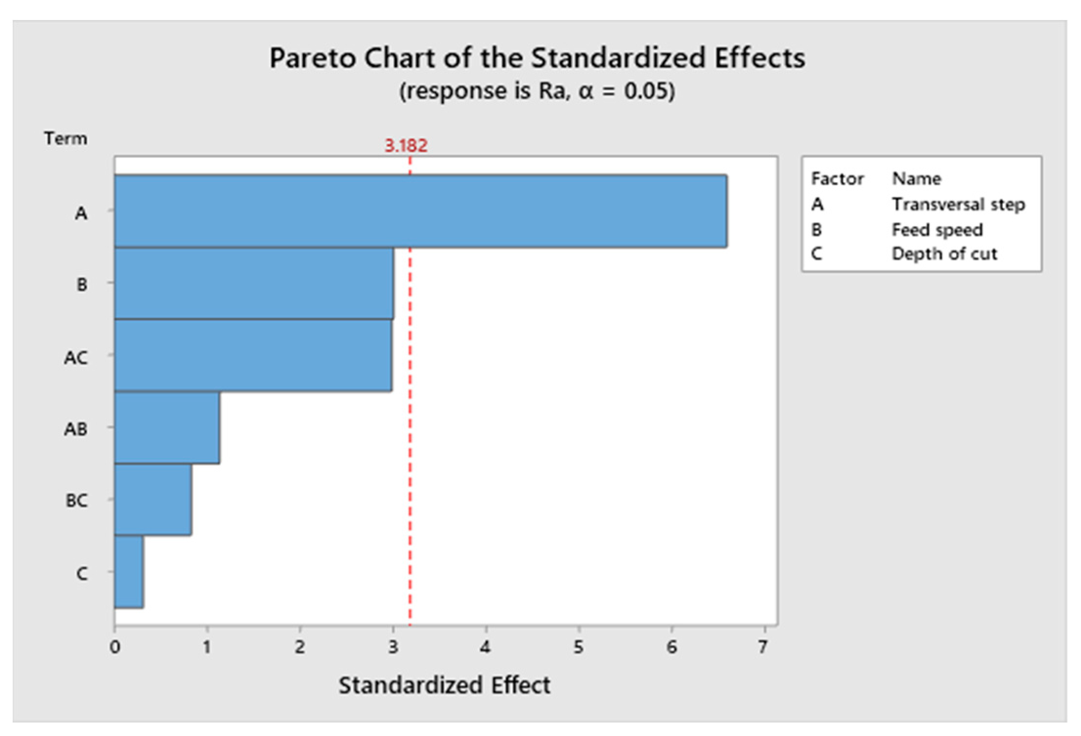
In this section, the statistical analysis is shown for Ra and the MRR.

3.4.1. Model for Ra

The coded coefficients for Ra are shown in

Table 3. Terms, effects, coefficient, SE coefficients, T-value, p-value, and VIF for Ra.

Term	Effect	Coef	SE Coef	T-Value	p-Value	VIF
Constant		0.4629	0.0107	43.39	0.000
Transversal step	0.1408	0.0704	0.0107	6.60	0.007	1.00
Feed speed	−0.0642	−0.0321	0.0107	−3.01	0.057	1.00
Depth of cut	0.0067	0.0034	0.0107	0.32	0.772	1.00
Transversal step·feed speed	−0.0242	−0.0121	0.0107	−1.14	0.338	1.00
Transversal step·depth of cut	0.0637	0.0319	0.0107	2.99	0.058	1.00
Feed speed·depth of cut	0.0178	0.0089	0.0107	0.83	0.466	1.00
Ct Pt		−0.0065	0.0204	−0.32	0.770	1.00

. The R²-sq parameter is 85.01%.

Figure 12 corresponds to the Pareto chart for Ra.

Within the range studied, the Ra roughness profile parameter value depends mainly on the transversal step, followed by feed speed and the mutual effect of the transversal step and depth of cut. Transversal step is known to influence surface roughness in flat grinding processes [36]. Feed speed and depth of cut also affect roughness [33,45].

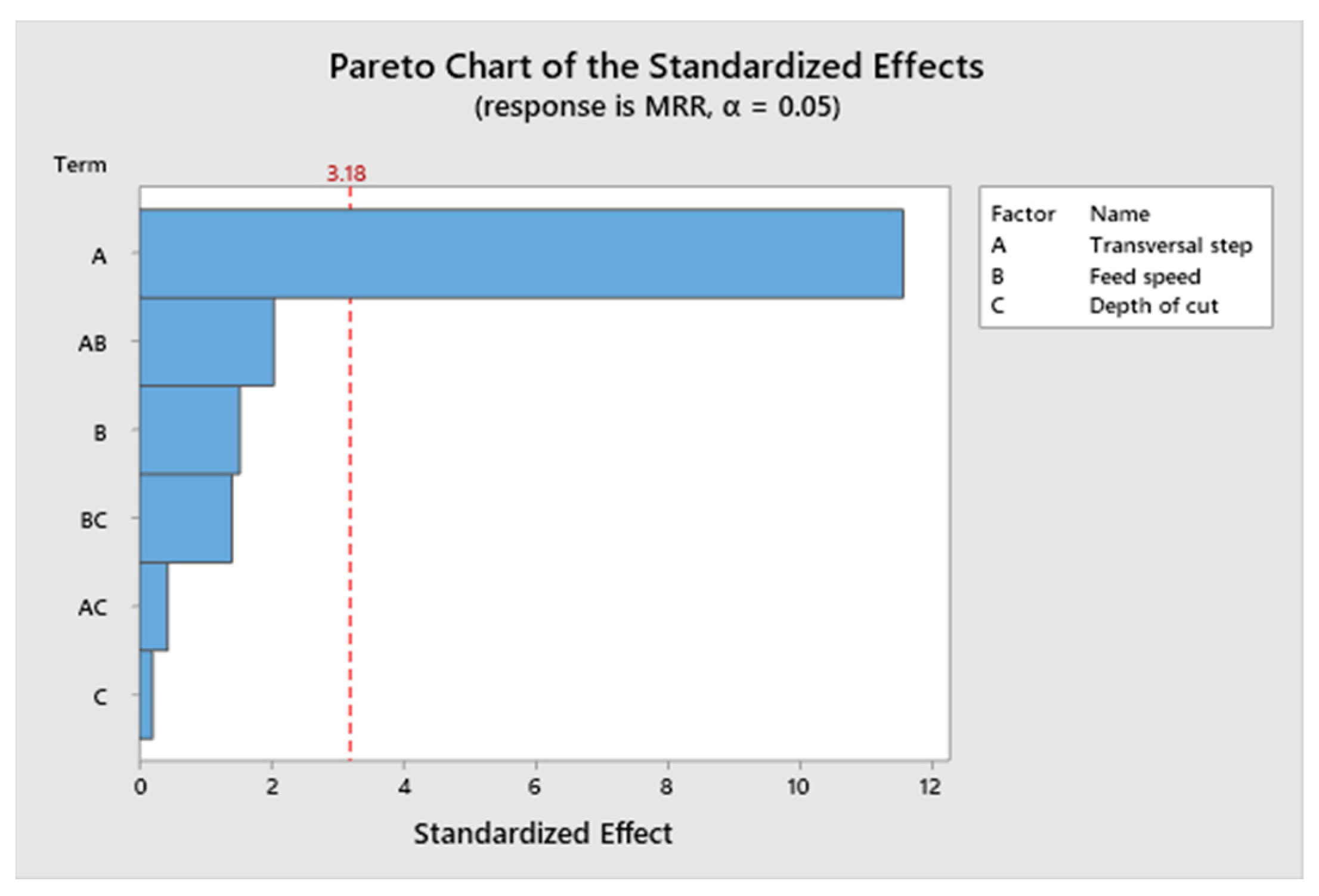
3.4.2. Model for the MRR

The coded coefficients for the MRR are shown in

Table 4. Terms, effects, coefficient, SE coefficients, T-value, p-value, and VIF for the MRR.

Constant		0.025587	0.000435	58.78	0.000
Transversal step	0.010075	0.005038	0.000435	11.57	0.001	1.00
Feed speed	0.001325	0.000663	0.000435	1.52	0.225	1.00
Depth of cut	−0.000175	−0.000087	0.000435	−0.20	0.854	1.00
Transversal step·feed speed	−0.001775	−0.000888	0.000435	−2.04	0.134	1.00
Transversal step·depth of cut	−0.000375	−0.000188	0.000435	−0.43	0.696	1.00
Feed speed·depth of cut	−0.001225	−0.000613	0.000435	−1.41	0.254	1.00
Ct Pt		−0.001421	0.000834	−1.70	0.187	1.00

. The R²-sq parameter is 93.27%.

Figure 13 corresponds to the Pareto chart for the MRR.

The MRR value depends mainly on the transversal step value followed by the mutual effect of the transversal step and feed speed. Feed is known to influence the material removal rate in grinding processes [36,46]. The characteristics of the grains, together with the depth of cut influence the type of mechanism that will mainly occur, among rubbing, plowing, and cutting. Cutting is preferred since it contributes greatly to material removal [47].

3.5. Multi-Objective Optimization

Table 5. Results of the multi-objective optimization.

Importance	Transversal Step (mm)	Feed Speed (mm/min)	Depth of Cut (mm)	MRR (mm/min)	Ra (µm)	Composite Desirability
Equal	9	20	0.010	0.0313	0.464	0.7385
10 times higher Ra	3	20	0.020	0.0216	0.330	0.8927
10 times higher MRR	9	20	0.010	0.0313	0.464	0.9464

contains the results of the multi-objective optimization using the Derringer–Suich function. Roughness was minimized, and the MRR was maximized. First, the same importance was given to both responses. Later, 10 times higher importance was used for each one of the responses.

If both responses are given the same importance, or if the MRR has higher importance, the recommendation is to use a high transversal step of 9 mm per longitudinal pass, a high feed speed of 20 mm/min, and a low depth of cut of 0.010 mm. On the contrary, if Ra has higher importance, a low transversal step of 3 mm per longitudinal pass and a high depth of cut of 0.020 mm should be selected. Kangharot et al. [48] optimized both the surface roughness and MRR in flat grinding processes. They recommend using a grit size 46, a depth of cut 0.20 mm, and a feed rate of 0.5404 mm/s (3.24 mm/min). However, they did not vary the cross-feed or transversal step.

4. Conclusions

In this work, the surface roughness, material removal rate, and energy of an AE signal in surface traverse grinding processes are analyzed. The main conclusions are as follows:

• Analysis of AE signal using filtration in three different frequency ranges is a useful method to analyze the grinding process. In this case, three modes were considered. As a general trend, the higher the depth of cut, the higher the energy values. The highest frequency of each frequency group tends to decrease with the depth of cut.
• The greatest influence on the Ra parameter is the transversal step followed by feed speed and the mutual effect of depth of cut and the transversal step.
• Within the ranges studied, the material removal rate depends mainly on the transversal step.
• In order to simultaneously obtain low roughness and a high MRR, a high transversal step and feed speed and a low depth of cut are recommended.

This research will contribute to the future monitorization of the grinding process from the analysis of the AE signal.

References

1. Klocke, F. Manufacturing Processes 2-Grinding, Honing, Lapping; Springer: Berlin/Heidelberg, Germany, 2009. [Google Scholar]
2. Liang, S.Y.; Shih, A.J. Analysis of Machining and Machine Tools; Springer: Berlin/Heidelberg, Germany, 2015. [Google Scholar]
3. Adeniji, D.; Oligee, K.; Schoop, J. A Novel Approach for Real-Time Quality Monitoring in Machining of Aerospace Alloy through Acoustic Emission Signal Transformation for DNN. J. Manuf. Mater. Process. 2022, 6, 18. [Google Scholar] [CrossRef]
4. Barylski, A.; Sender, P. The proposition of an automated honing cell with advanced monitoring. Machines 2020, 8, 70. [Google Scholar] [CrossRef]
5. Ferrando Chacón, J.L.; Fernández de Barrena, T.; García, A.; Sáez de Buruaga, M.; Badiola, X.; Vicente, J. A Novel Machine Learning-Based Methodology for Tool Wear Prediction Using Acoustic Emission Signals. Sensors 2021, 21, 5984. [Google Scholar] [CrossRef] [PubMed]
6. Rimpault, X.; Chatelain, J.F.; Klemberg-Sapieha, J.E.; Balazinski, M. Fractal Analysis of Cutting Force and Acoustic Emission Signals during CFRP Machining. Procedia CIRP 2016, 46, 143–146. [Google Scholar] [CrossRef]
7. Gómez, M.P.; Hey, A.M.; Ruzzante, J.E.; D’Attellisc, C.E. Tool wear evaluation in drilling by acoustic emission. Phys. Procedia 2010, 3, 819–825. [Google Scholar] [CrossRef]
8. Kuntoğlu, M.; Aslan, A.; Pimenov, D.Y.; Usca, Ü.A.; Salur, E.; Gupta, M.K.; Mikolajczyk, T.; Giasin, K.; Kapłonek, W.; Sharma, S. A review of indirect tool condition monitoring systems and decision-making methods in turning: Critical analysis and trends. Sensors 2021, 21, 108. [Google Scholar] [CrossRef]
9. Murat, Z.; Brezak, D.; Augustin, G.; Majetic, D. Frequency domain analysis of acoustic emission signals in medical drill wear monitoring. In Proceedings of the 10th International Joint Conference on Biomedical Engineering Systems and Technologies (BIOSTEC 2017), Porto, Portugal, 21–23 February 2017; Volume 4, pp. 173–177. [Google Scholar]
10. Nahornyi, V.; Panda, A.; Valíček, J.; Harničárová, M.; Kušnerová, M.; Pandová, I.; Legutko, S.; Palková, Z.; Lukáč, O. Method of Using the Correlation between the Surface Roughness of Metallic Materials and the Sound Generated during the Controlled Machining Process. Materials 2022, 15, 823. [Google Scholar] [CrossRef]
11. Sio-Sever, A.; Lopez, J.M.; Asensio-Rivera, C.; Vizan-Idoipe, A.; de Arcas, G. Improved Estimation of End-Milling Parameters from Acoustic Emission Signals Using a Microphone Array Assisted by AI Modelling. Sensors 2022, 22, 3807. [Google Scholar] [CrossRef]
12. Zhang, Y.; Qi, X.; Wang, T.; He, Y. Tool Wear Condition Monitoring Method Based on Deep Learning with Force Signals. Sensors 2023, 23, 4595. [Google Scholar] [CrossRef]
13. The Ho, Q.N.; Do, T.T.; Minh, P.S.; Nguyen, V.T.; Nguyen, V.T.T. Turning Chatter Detection Using a Multi-Input Convolutional Neural Network via Image and Sound Signal. Machines 2023, 11, 644. [Google Scholar] [CrossRef]
14. Huda, F.; Darman, D.; Rusli, M. Chatter detection in turning process using sound signal and simple microphone. IOP Conf. Ser. Mater. Sci. Eng. 2020, 830, 42027. [Google Scholar] [CrossRef]
15. Nikhare, C.P.; Conklin, C.; Loker, D.R. Understanding acoustic emission for different metal cutting machinery and operations. J. Manuf. Mater. Process. 2017, 1, 7. [Google Scholar] [CrossRef]
16. Nourizadeh, R.; Rezaei, S.M.; Zareinejad, M.; Adibi, H. Comprehensive investigation on sound generation mechanisms during machining for monitoring purpose. Int. J. Adv. Manuf. Technol. 2022, 121, 1589–1610. [Google Scholar] [CrossRef]
17. Papacharalampopoulos, A.; Stavropoulos, P.; Doukas, C.; Foteinopoulos, P.; Chryssolouris, G. Acoustic emission signal through turning tools: A computational study. Procedia CIRP 2013, 8, 426–431. [Google Scholar] [CrossRef]
18. Perrelli, M.; Cosco, F.; Gagliardi, F.; Mundo, D. In-Process Chatter Detection Using Signal Analysis in Frequency and Time-Frequency Domain. Machines 2022, 10, 24. [Google Scholar] [CrossRef]
19. Chen, G.; Wang, Z. A signal decomposition theorem with Hilbert transform and its application to narrowband time series with closely spaced frequency components. Mech. Syst. Signal Process. 2012, 28, 258–279. [Google Scholar] [CrossRef]
20. Leaman, F.; Vicuña, C.M.; Clausen, E. Potential of Empirical Mode Decomposition for Hilbert Demodulation of Acoustic Emission Signals in Gearbox Diagnostics. J. Vib. Eng. Technol. 2022, 10, 621–637. [Google Scholar] [CrossRef]
21. Amarnath, M.; Praveen Krishna, I.R. Local fault detection in helical gears via vibration and acoustic signals using EMD based statistical parameter analysis. Meas. J. Int. Meas. Confed. 2014, 58, 154–164. [Google Scholar] [CrossRef]
22. Deja, M. Method of Monitoring of the Grinding Process with Lapping Kinematics Using Audible Sound Analysis. J. Mach. Eng. 2022, 22, 157255. [Google Scholar] [CrossRef]
23. Sender, P.; Buj-Corral, I. Influence of Honing Parameters on the Quality of the Machined Parts and Innovations in Honing Processes. Metals 2023, 13, 140. [Google Scholar] [CrossRef]
24. Warren Liao, T. Feature extraction and selection from acoustic emission signals with an application in grinding wheel condition monitoring. Eng. Appl. Artif. Intell. 2010, 23, 74–84. [Google Scholar] [CrossRef]
25. Pilný, L.; Bissacco, G.; De Chiffre, L.; Ramsing, J. Acoustic Emission Based In-process Monitoring in Robot Assisted Polishing. Int. J. Comput. Integr. Manuf. 2016, 29, 1218–1226. [Google Scholar] [CrossRef]
26. Mirifar, S.; Kadivar, M.; Azarhoushang, B. First steps through intelligent grinding using machine learning via integrated acoustic emission sensors. J. Manuf. Mater. Process. 2020, 4, 35. [Google Scholar] [CrossRef]
27. Nguyen, V.H.; Vuong, T.H.; Nguyen, Q.T. Feature representation of audible sound signal in monitoring surface roughness of the grinding process. Prod. Manuf. Res. 2022, 10, 606–623. [Google Scholar] [CrossRef]
28. Hatami, O.; Sayadi, D.; Razbin, M.; Adibi, H. Optimization of Grinding Parameters of Tool Steel by the Soft Computing Technique. Comput. Intell. Neurosci. 2022, 2022, 3042131. [Google Scholar] [CrossRef] [PubMed]
29. Demir, H.; Gullu, A.; Ciftci, I.; Seker, U. An investigation into the influences of grain size and grinding parameters on surface roughness and grinding forces when grinding. Stroj. Vestnik/J. Mech. Eng. 2010, 56, 447–454. [Google Scholar]
30. Wang, C.; Wang, G.; Shen, C. Analysis and Prediction of Grind-Hardening Surface Roughness Based on Response Surface Methodology-BP Neural Network. Appl. Sci. 2022, 12, 12680. [Google Scholar] [CrossRef]
31. Wen, X.; Li, J.; Gong, Y. Simulation and experimental research on grinding force and grinding surface quality of TiC-coated micro-grinding tools. Int. J. Adv. Manuf. Technol. 2023, 128, 1337–1351. [Google Scholar] [CrossRef]
32. Ying, J.; Yin, Z.; Zhang, P.; Zhou, P.; Zhang, K.; Liu, Z. An Experimental Study of the Surface Roughness of SiCp/Al with Ultrasonic Vibration-Assisted Grinding. Metals 2022, 12, 1730. [Google Scholar] [CrossRef]
33. Kwak, J.S.; Ha, M.K. Neural network approach for diagnosis of grinding operation by acoustic emission and power signals. J. Mater. Process. Technol. 2004, 147, 65–71. [Google Scholar] [CrossRef]
34. Ruzzi, R.d.S.; da Silva, R.B.; da Silva, L.R.R.; Machado, Á.R.; Jackson, M.J.; Hassui, A. Influence of grinding parameters on Inconel 625 surface grinding. J. Manuf. Process. 2020, 55, 174–185. [Google Scholar] [CrossRef]
35. Ma, L.J.; Gong, Y.D.; Chen, X.H.; Duan, T.Y.; Yang, X.Y. Surface roughness model in experiment of grinding engineering glass-ceramics. Proc. Inst. Mech. Eng. Part B J. Eng. Manuf. 2014, 228, 1563–1569. [Google Scholar] [CrossRef]
36. Patel, D.K.; Goyal, D.; Pabla, B.S. Optimization of parameters in cylindrical and surface grinding for improved surface finish. R. Soc. Open Sci. 2018, 5, 171906. [Google Scholar] [CrossRef]
37. König, W.; von Arciszewski, A. Continuous Dressing-Dressing Conditions Determine Material Removal Rates and Workpiece Quality. CIRP Ann.-Manuf. Technol. 1988, 37, 303–307. [Google Scholar] [CrossRef]
38. Kumar, P.; Kumar, A.; Singh, P. Optimization of Process Parameters in Surface Grinding using Response Surface Methodology. IJRMET 2013, 3, 245–252. [Google Scholar]
39. Walton, I.M.; Stephenson, D.J.; Baldwin, A. The measurement of grinding temperatures at high specific material removal rates. Int. J. Mach. Tools Manuf. 2006, 46, 1617–1625. [Google Scholar] [CrossRef]
40. Wei, C.; He, C.; Chen, G.; Sun, Y.; Ren, C. Material removal mechanism and corresponding models in the grinding process: A critical review. J. Manuf. Process. 2023, 103, 354–392. [Google Scholar] [CrossRef]
41. Singh, K.; Singh, B.; Kumar, M. Experimental Investigation of Machining Characteristics of AISI D3 Steel with Abrasive Assisted Surface Grinding. Int. Res. J. Eng. Technol. 2015, 2, 269. [Google Scholar]
42. Yin, G.; Wang, J.; Guan, Y.; Wang, D.; Sun, Y. The prediction model and experimental research of grinding surface roughness based on AE signal. Int. J. Adv. Manuf. Technol. 2022, 120, 6693–6705. [Google Scholar] [CrossRef]
43. Webster, J.; Marinescu, I.; Bennett, R.; Lindsay, R. Acoustic Emission for Process Control and Monitoring of Surface Integrity during Grinding. CIRP Ann.-Manuf. Technol. 1994, 43, 299–304. [Google Scholar] [CrossRef]
44. Klocke, F. Grinding. In Manufacturing Processes 2; Springer: Berlin/Heidelberg, Germany, 2009. [Google Scholar]
45. Aguiar, P.R.; Cruz, C.E.; Paula, W.C.; Bianchi, E.C. Predicting Surface Roughness in Grinding Using Neural Networks. In Advances in Robotics, Automation and Control; IntechOpen Limited: London, UK, 2008. [Google Scholar]
46. Zhang, S.; Zhang, G.; Ran, Y.; Wang, Z.; Wang, W. Multi-objective optimization for grinding parameters of 20CrMnTiH gear with ceramic microcrystalline corundum. Materials 2019, 12, 1352. [Google Scholar] [CrossRef] [PubMed]
47. Öpöz, T.T.; Chen, X. Experimental study on single grit grinding of Inconel 718. Proc. Inst. Mech. Eng. Part B J. Eng. Manuf. 2015, 229, 713–726. [Google Scholar] [CrossRef]
48. Khangarot, H.; Sharma, S.; Vates, U.K.; Singh, G.K.; Kumar, V. Optimization of surface grinding process parameters through RSM. In Proceedings of the International Conference on Modern Research in Aerospace Engineering. Lecture Notes in Mechanical Engineering; Singh, S., Raj, P., Tambe, S., Eds.; Springer: Singapore, 2018; pp. 291–302. [Google Scholar] [CrossRef]
Figure 1. Tangential grinding machine used in the experiments: 1—CNC grinder, 2—computer with Matlab and Audacity software, and 3—control panel of the CNC grinder.
Machines 12 00110 g001
Figure 2. Experimental setup. 1—display, 2—workpiece, 3—directional condenser microphone, 4—laptop with a software package (including Matlab, Audacity, Minitab), and 5—control panel.
Machines 12 00110 g002
Figure 3. Measurement of the overall dimension of the ground workpiece: 1—measured workpiece and 2—digital micrometer.
Machines 12 00110 g003
Figure 4. Control panel of the CNC grinder—1 and computer with Matlab and Audacity software—2.
Machines 12 00110 g004
Figure 5. Procedure to obtain the three filtered signals.
Machines 12 00110 g005
Figure 6. Original sound recorded during the grinding process of experiment number 1.
Machines 12 00110 g006
Figure 7. Original sound and IMF 1 of experiment 1.
Machines 12 00110 g007
Figure 8. FFT and IMF1 of the sound signal of experiment 1.
Machines 12 00110 g008
Figure 9. Power spectrum of the frequency range 150 Hz ÷ 1000 Hz, corresponding to Ey1, with dominant frequency X = 0.83 kHz and max amplitude value Y = −37.63 dB.
Machines 12 00110 g009
Figure 10. Power spectrum of the frequency range 1 kHz ÷ 3.5 kHz, corresponding to Ey2, with dominant frequency X = 1.97 kHz and max amplitude value Y = −47.82 dB.
Machines 12 00110 g010
Figure 11. Power spectrum of the frequency range 3.5 k Hz ÷ 10.5 k Hz, corresponding to Ey3, with dominant frequency X = 6.49 kHz and max amplitude value Y = −48.37 dB.
Machines 12 00110 g011
Figure 12. Pareto chart for Ra.
Machines 12 00110 g012
Figure 13. Pareto chart for the MRR.
Machines 12 00110 g013