Deep Learning-Enhanced Small-Sample Bearing Fault Analysis Using Q-Transform and HOG Image Features in a GRU-XAI Framework

Abstract

Timely prediction of bearing faults is essential for minimizing unexpected machine downtime and improving industrial equipment’s operational dependability. The Q transform was utilized for preprocessing the sixty-four vibration signals that correspond to the four bearing conditions. Additionally, statistical features, also known as attributes, are extracted from the Histogram of Oriented Gradients (HOG). To assess these features, the Explainable AI (XAI) technique employed the SHAP (Shapely Additive Explanations) method. The effectiveness of the GRU, LSTM, and SVM models in the first stage was evaluated using training and tenfold cross-validation. The SSA optimization algorithm (SSA) was employed in a subsequent phase to optimize the hyperparameters of the algorithms. The findings of the research are rigorously analyzed and assessed in four specific areas: the default configuration of the model, the inclusion of selected features using XAI, the optimization of hyperparameters, and a hybrid technique that combines SSA and XAI-based feature selection. The GRU model has superior performance compared to the other models, achieving an impressive accuracy of 98.2%. This is particularly evident when using SSA and XAI-informed features. The subsequent model is the LSTM, which has an impressive accuracy rate of 96.4%. During tenfold cross-validation, the Support Vector Machine (SVM) achieves a noticeably reduced maximum accuracy of 84.82%, even though the hybrid optimization technique shows improvement. The results of this study usually show that the most effective model for fault prediction is the GRU model, configured with the attributes chosen by XAI, followed by LSTM and SVM.

1. Introduction

Bearings are essential parts used in various industries because they allow multiple components to move smoothly and efficiently together. Bearings help to evenly distribute loads by supporting shafts, axles, or other moving parts, reducing heavy wear and tear on machinery. Various types of stresses, such as mechanical loads, vibrations, and temperature changes, subject bearings to wear and tear over time, leading to bearing faults. These faults can lead to machine downtime, increased maintenance costs, and even safety hazards. Therefore, timely detection and diagnosis of bearing faults are crucial to prevent equipment failure and optimize the overall performance of machinery [1]. A variety of methods are used for bearing condition monitoring to evaluate their state of health and identify possible problems before they become serious malfunctions. One of the most used techniques is vibration analysis, which measures and examines bearing vibrations to find unusual patterns like misalignment, imbalance, or bearing component failures. Signal processing is important for removing noise from signals because it pulls out useful information from noisy sensor data and makes it easier to find fault patterns. Wavelet transformations (WT), empirical mode decomposition (EMD), and Walsh–Hadamard transform (WHT) are prominent approaches [2,3,4]. Fast Fourier transform (FFT) converts vibration signals into the frequency domain, detecting abnormal frequencies related to bearing faults [5]. Wavelet transform (WT) analyzes signals in both time and frequency domains, offering superior time-frequency resolution and detecting transient fault signals [6]. Ensemble Empirical Mode Decomposition (EEMD) decomposes bearing signals into different time scales to extract relevant information, addressing issues like mode mixing and spectral leakage present in conventional EMD [7]. Since bearings have a high failure rate, Zhu et al. [8] proposed a novel feature fusion approach for bearing fault feature extraction and diagnostics. The bearing signal time-frequency data is first extracted as a characteristic matrix using the Wavelet Packet Transform (WPT). To increase fault detection accuracy and eliminate superfluous features, this matrix is modified by employing Multi-weight Singular Value Decomposition (MWSVD), which is based on singular value contribution rates and entropy weight. Li et al. [9] investigated a methodology based on encoder signals and combined it with a locally weighted multi-instance multi-label (LWMIML) network to create feature vectors and find associations between features and defect categories. The effectiveness of the study was validated using data from fault simulation test rigs, demonstrating its potential as an affordable substitute for intelligent fault diagnosis systems. Recently multi-fault diagnosis strategy based on iterative generalized demodulation is reported [10]. The methodology proposes a novel diagnosis technique guided by the instantaneous fault characteristic frequency under varying speeds. The authors compared both simulated and experimental results to demonstrate the diagnosis’s effectiveness. In another study, adaptive thresholding and coordinate attention-based tree-inspired network was proposed to detect healthy conditions of bearings [11]. Moreover, a frequency-chirprate synchrosqueezing operator was introduced to analyze the time-frequency representation of bearings faults. The diagnosis accuracy is verified with simulated and experimental signals [12]. Kiakojouri et al. [13] proposed a cepstrum pre-whitening-based filtration technique to identify the impulsive features associated with various bearing faults. The outcomes additionally demonstrate its efficacy in identifying several bearing faults that occur under various bearing operating conditions.

Due to their superior ability to handle complicated and non-stationary data patterns, which are frequently present in vibration signals, machine learning (ML) and deep learning (DL) techniques have revolutionized the diagnosis of bearing faults. Conventional methods of signal processing, such as the Fourier, Wavelet, and Empirical Mode Decomposition transforms, concentrate on taking features out of the signal by using mathematical models and predetermined rules [14,15]. Even while these techniques are good at isolating specific frequency components and transient features, they frequently fail to capture the complex, high-dimensional connections present in the data, especially when operating circumstances and noise levels vary. On the other hand, massive volumes of historical data are utilized by ML and DL techniques to extract optimal features and decision boundaries straight from the data. With more accuracy and dependability, these models can automatically adjust to complicated data, spotting minute patterns and abnormalities that can point to bearing abnormalities [16]. Pham et al. [17] demonstrate a simplified CNN-based embedded device diagnosis procedure that uses acoustic emission data to classify faults. Through the use of a MobileNet-v2 model that has been pruned and tuned for lower system resource utilization, this technique substantially decreases computing costs. A unique classification technique to identify faults with small sample datasets is presented by Yang et al. [18]. This technique makes use of a triplet embedding connection between each stage of recognizing faults and the extraction of features in the categorization of vibration data. Comparison tests using stacked autoencoders, stacked denoising autoencoders, and traditional CNN techniques verify the effectiveness of the approach and demonstrate improved fault diagnosis performance in small sample sizes.

The decision to choose features is critical because it identifies and retains just the most relevant informative characteristics from signals, considerably improving the efficacy of classification algorithms. When it applies to bearing fault diagnosis, unnecessary complexity in the form of ineffective features may hinder meaningful trends, cause overfitting, and complicate classification models. Feature selection techniques minimize the dimensionality of the dataset, making the model simpler, easier to understand, and faster to train. Feature selection also helps the classification algorithm focus on the dataset’s most important features that are indicative of bearing failures. This makes it easier to identify small but important fault attributes. As a result, feature selection becomes an important strategy for enhancing the effectiveness of bearing fault diagnosis techniques by carefully removing unnecessary information and emphasizing key characteristics, guaranteeing that classification models are effective and very accurate in forecasting bearing health states. Li et al. [19] presented a sophisticated framework to diagnose hybrid faults in gearboxes. A new two-step feature selection procedure combining filter and wrapper techniques using mutual information and non-dominated sorting genetic algorithms II (NSGA-II) was evaluated. Karabadji et al. [20] combine attribute selection with data sampling to improve the process of choosing relevant attributes and database elements, thus making it easier to develop decision rules for fault diagnosis in rotating machinery. Experimental comparisons on ten reference datasets prove the effectiveness of this strategy and highlight its superiority over conventional decision tree-building techniques. Rajeswari et al. [21] describe a novel approach to gearbox diagnosis that uses vibration data from test equipment for early defect detection. To reduce computing demands, the study optimizes feature selection using both a rough set-based technique and a genetic algorithm (GA). Gao et al. [22] proposed a causal feature network-based feature selection technique for composite fault diagnosis in bearing. As demonstrated by experimental results, a very high accuracy was reported.

With its intrinsic transparency and interpretability, explainable AI (XAI) represents a revolutionary shift from traditional wrapper and metaheuristic optimization-based methods in the field of feature selection. Conventional techniques, although successful in recognizing significant feature subsets, frequently function as “black boxes”, providing a limited understanding of the reasoning underlying feature relevance and selection choices. This obscurity can be a major disadvantage, particularly in fields like healthcare, finance, etc., that demand strict validation and comprehension of model behavior. On the other hand, XAI-based feature selection methods shed light on the selection procedure and offer concise justifications for the significance of particular traits. This promotes a deeper comprehension of the underlying processes being modeled, in addition to increasing trust and confidence. XAI models can identify links in the data that were previously overlooked, which can lead to discoveries and even direct future studies. As a result, XAI-based feature selection stands out as a better strategy that combines transparency and performance while encouraging a more in-depth interaction with the model’s decision-making processes. To meet the essential requirement for transparency in Industry 4.0’s Fault Detection and Diagnosis (FDD) procedures for chemical process systems, Harinarayan et al. [23] presented an inventive framework called Explainable Fault Detection, Diagnosis, and Correction (XFDDC). When the framework was applied, an enhanced fault detection rate and F1 score were observed. Moreover, Meas et al. [24] presented a novel use of XAI for assisting HVAC engineers to efficiently identify faults in air handling units. The SHAP technique was used in the study to improve explainability and visualize the temporal evolution of the important features. The system’s explanatory power was confirmed after validation with actual experimental data.

The Q transform provides improved time-frequency resolution and adaptability to non-stationary data, which sets it apart from other classic signal processing transforms. The Q transform specializes at precisely temporally resolving both high- and low-frequency components and offers rich, informative features that capture the fundamental dynamics of bearing failures, which improves the model’s capacity to learn and generalize from sparse experimental datasets when paired with deep learning techniques like LSTM, GRU, and SVM. In small sample numbers, where it becomes difficult to capture the crucial fault characteristics, this synergy is very effective. In addition, the innovative use of Explainable AI (XAI) for feature selection in LSTM and GRU frameworks is a major breakthrough in the identification of bearing faults. By emphasizing the most pertinent features obtained from the Q transform, XAI not only increases model interpretability but also helps with model transparency and reliability, filling a significant gap in the literature. This integrated technique, which combines the power of XAI-enhanced deep learning models with the Q transform, guarantees reliable, accurate, and explicable issue detection even in situations when data availability is limited. As such, it represents a significant advancement in predictive maintenance solutions. The authors have made noteworthy contributions to the methodology and assessment of bearing fault diagnosis through the following innovations:

• The Q transform, a robust time-frequency analysis technique, is applied to extract features from raw signal data, effectively capturing both temporal and frequency-domain information pertinent to bearing fault detection. To enhance interpretability, XAI techniques are applied to identify and highlight the most relevant features derived from the Q transform.
• For performance comparison across various model architectures, this study employs three distinct machine learning techniques—SVM, LSTM, and GRU—to predict bearing defects.
• The novel utilization of LSTM and GRU as XAI models for bearing fault diagnosis is explored, significantly enhancing the transparency and robustness of predictive maintenance technologies.
• The methodology is further refined by incorporating SSA optimization for hyperparameter tuning, alongside XAI-based feature selection. This approach not only optimizes the machine learning models but also enhances their interpretability and effectiveness in fault prediction.
• The robustness and generalization of the models are meticulously validated utilizing tenfold cross-validation, ensuring superior performance across different models.

Figure 1 illustrates the bearing fault diagnosis methodology based on the proposed framework.

2. Materials and Methods

2.1. Discrete Cosine Transform (DCT)

The discrete cosine transform (DCT) is a common signal processing method that breaks down a signal into a sum of cosine functions that oscillate at different frequencies. Its basic idea is to represent a signal in the frequency domain by converting a series of data points into a sum of cosine functions with different amplitudes and frequencies. It is very useful because it compactly reflects the signal energy, focusing mainly on a few coefficients. The capacity of DCT to extract and amplify signal features becomes critical in fault diagnosis, particularly in mechanical and electrical systems where vibrational and signal analysis are critical [25]. For instance, vibration signals from rotating machinery’s gears or bearings contain frequency components directly linked to the fault features. When applied to a noisy signal condition, DCT may effectively emphasize specific fault-induced frequencies, which helps with accurate problem identification and classification. DCT’s compact energy description feature makes it possible to identify anomalies, wear, or failure mechanisms in equipment by extracting significant features from raw diagnostic data and analyzing them effectively [26]. As a result, using DCT in fault diagnosis procedures improves the precision and dependability of problem detection, enabling early warning systems and preventative maintenance procedures to reduce expensive downtime and equipment failures. The DCT of a noisy signal x[n], where n = 0, 1, 2, …, N − 1 and k = 0, 1, 2, …, N − 1, is calculated as follows:

$$X\left[k\right]={\sum }_{n=0}^{N-1}x\left[n\right]·\mathrm{c}\mathrm{o}\mathrm{s}(\frac{\pi }{N} \left(n+\frac{1}{2} \right)k)$$

(1)

where N is the total number of samples in the signal and k = 0, 1, 2, …, N − 1.

DCT is highly advantageous in the diagnosis of bearing faults due to several intrinsic properties that align well with the need for effective fault detection in rotating machinery. Most notable is DCT’s energy compaction feature, which focuses most signal energy into a few coefficients, thereby enhancing subtle fault-induced changes in vibration signals. Additionally, DCT decorrelates signal data, simplifying recurrent fault signal patterns caused by mechanical activities and making anomaly identification easier.

2.2. Q Transform

A powerful tool in signal processing, the Q transform is a variation of the Fourier transform. It is particularly useful because it can provide a configurable and adaptable time-frequency description for non-stationary data. By adding a quality factor Q into the Fourier transform, these mathematical techniques allow for the adjustment of the analysis’s temporal and frequency resolution [27]. The Q transform’s versatility is especially helpful in diagnosing bearing faults. By varying Q, analysts can identify specific signal components that correspond to common defect signs, such as cracks or spalls in bearing races. The procedure is carried out algorithmically by first applying the Q transform to decompose the vibration signals of the bearings and produce time-frequency representations. Using ML models to categorize these features into distinct fault categories according to their distinct time-frequency characteristics is a common stage in the process. As a result, the Q transform not only helps with accurate problem identification but also advances knowledge of defect mechanisms, which eventually boosts the dependability and effectiveness of mechanical systems.

2.3. HOG Features

Histogram of Oriented Gradients (HOG) features, a category of image processing algorithms, extract useful information from images by considering the orientation and distribution of edge directions throughout localized regions of the image. The basic idea behind HOG features is to create a histogram of the edge orientations or gradient directions of the pixels within each of the small, connected sections, or cells, that constitute the image. The combination of these histograms then represents the descriptor or feature set for the full image. By highlighting the existence of edges, this technique is especially good at collecting SHAP and texture information, which is essential for tasks involving object detection, recognition, and classification [28]. When used for fault identification, HOG attributes can be highly beneficial, especially in scenarios requiring defect analysis or visual inspection. For instance, HOG features can help precisely identify the structures or textures linked to different types of defects in automated visual assessment for keeping an eye on wear, spalls, or cracks in machinery parts by capturing the different edge orientations that are linked to each fault category. This feature makes it easier to categorize abnormalities and errors in mechanical components using visual data, which improves the effectiveness and dependability of fault diagnosis operations. Derivative masks, such as Sobel operators, are used to compute the gradients G_x and G_y in the horizontal and vertical axes, respectively, for image I:

$$G_x=I\left(x+1, y\right)-I(x-1, y)$$

(2)

$$G_{y }=I\left(x, y+1\right)-I(x, y-1)$$

(3)

The gradient magnitude (M) and direction (θ) are then calculated as follows:

$$M\left(x, y\right)=\sqrt{G_x^2+G_y^2}$$

(4)

$$\theta \left(x, y\right)=a\tan 2(G_y, G_x)$$

(5)

where atan2 ensures that the direction is calculated with the appropriate quadrant in consideration.

By binning the gradient directions (θ) into a predetermined number of orientation bins, a histogram of gradient directions is created for each cell. The gradient magnitude M typically evaluates the vote for the histogram bins, and a Gaussian window may also weight it to give the pixels in the middle of the cell greater significance. Blocks of many neighboring cells are combined to form larger units (e.g., 2 × 2 cells). To lessen the impact of changes, the histograms of every cell in each block are concatenated and then normalized. One popular normalization technique is the L2 norm, expressed as follows:

$$v=\frac{v}{\sqrt{{‖v‖}_2^2+{ϵ}^2}}$$

(6)

where ϵ is a tiny constant to prevent divisions by zero and v is the block’s concatenation histogram vector. The final HOG feature descriptors are created by concatenating the normalized block histograms.

2.4. Machine Learning Techniques

ML is the convergence of computer science and statistics, allowing computers to learn from data without explicit programming. Through a process known as training, ML programs reveal hidden patterns and correlations within data, in contrast to classical algorithms that follow pre-established rules. A feature vector consisting of labeled data with a desired output for each data point is fed into the system during training [29,30]. Through repeated data analysis, the algorithm improves its internal model, allowing it to carry out operations like classification, regression, and cluster analysis. The goal of this research is to derive significant insights from the fault data gathered during our investigation using ML methodologies. This will facilitate the use of a data-driven strategy to improve fault pattern recognition.

2.4.1. Support Vector Machine

SVMs have become well known as efficient methods for classification in the field of supervised learning. Finding the best hyperplane inside a high-dimensional feature space is the goal of the SVM method. This hyperplane successfully divides data points into different classes by serving as a decision boundary. Maximizing the margin between the hyperplane and the closest data points from each class—also referred to as support vectors—is the fundamental idea behind SVMs. These support vectors play a crucial role in defining the classification model. A larger margin indicates a stronger judgment border that is less susceptible to noise or omitted data points. Data points project into a higher-dimensional space, even if the source data are located in a lower-dimensional environment. This allows SVMs to manage non-linear feature associations that a hyperplane cannot divide in the original space [31]. The decision function of an SVM can be expressed as follows:

f(x) = w^T ∗ Φ(x) + b

(7)

where the weight vector w defines the positioning of the hyperplane in the space of multiple dimensions. The mapping function Φ(x) represents how the data point x is transformed into a space with high dimensions, and the bias term b indicates how the hyperplane is shifted. This research employs SVMs due to their proficiency in managing high-dimensional data and their ability to depict the non-linear correlations among the features in our dataset. This property is quite helpful for proposed bearing fault diagnosis.

2.4.2. Long Short-Term Memory

The Long Short-term Memory (LSTM) paradigm represents an enhanced iteration of the recurrent neural network (RNN) architecture. The LSTM model is very suitable for problems involving sequence prediction and demonstrates exceptional performance in preserving long-term dependencies. The strength of the algorithm rests in its capacity to comprehend the dependence on order, which is essential for addressing challenging issues such as machine translation and recognition of speech. Conventional RNNs propagate a single hidden state over time, which presents challenges for the network in learning long-term dependencies. The models tackle this issue by incorporating a memory cell, which acts as a receptacle capable of retaining information over a prolonged period of time [32]. The control mechanism of the memory cell consists of three distinct gates, namely the input gate, the forget gate, and the output gate. The aforementioned gates are responsible for determining the inclusion, exclusion, and output of information within the memory cell. The forget gate eliminates information that is no longer relevant to the cell state. The gate receives two inputs, x_t and h_t−1, which are multiplied with weight matrices, and then bias is added. An activation function is applied to the resultant, resulting in a binary output. If the output for a specific cell state is 0, the information is erased, but for output 1, the information is preserved for future utilization. The formula for the forget gate is as follows:

$$f_{t }=\sigma (W_{f }\left[h_{t-1},x_t \right]+b_f)$$

(8)

where the weight matrix linked with the forget gate is denoted as W_f. The combination of the current input and the prior hidden state is denoted as [h_t−1, x_t]. The bias corresponding to the forget gate is denoted as b_f, whereas the sigmoid activation function is represented by σ.

The input gate is responsible for incorporating valuable information into the cell state. Initially, the data is regulated through the utilization of the sigmoid function, which subsequently filters the values to be retained, analogous to the forget gate. This process involves the utilization of inputs h_t−1 and x_t. The tanh function is preferred for this purpose due to its ability to center the data around zero and represent both positive and negative values, which is crucial for maintaining a balanced gradient flow and stabilizing the learning process. The input gate equation is as follows:

$$i_t=\sigma \left(W_{i }\left[h_{t-1}, x_t\right]+b_i\right)$$

(9)

$${\widehat{C}}_t=\tanh \left(W_c\left[h_{t-1}, x_t\right]+b_c\right)$$

(10)

C_t represents the updated candidate values.

The output gate is responsible for obtaining valuable information about the current cell state and presenting it as output. Initially, the generation of a vector is achieved through applying the tanh function to the cell. The data are subsequently regulated by the utilization of the sigmoid function and filtered based on the values to be retained, which are determined by the inputs h_t−1 and x_t. Subsequently, the vector values and the controlled values undergo multiplication to be transmitted as an output and input to the subsequent cell. The equation governing the output gate is as follows:

$$o_t=\mathsf{\sigma }\left(W_{o }\left[h_{t-1}, x_t\right]+b_o\right)$$

(11)

The following are the main reasons why the tanh function is preferred in the framework of LSTM networks: With an output range of −1 to +1, the tanh function enables the network to express an extensive range of values, comprising positive as well as negative values, providing an additional centered and equitable activation. This zero-centeredness aids in preserving a balanced flow of gradients and sustaining the learning process. By balancing the gradients of the tanh function around zero, the issue of vanishing gradients throughout training is mitigated. This is essential for LSTM networks’ basic characteristic of retaining long-term dependencies in sequential data.

2.4.3. Gated Recurrent Unit

GRUs are a robust structure in RNNs that are meant to efficiently process sequential input, similar to LSTM networks. LSTMs employ distinct forget and input gates, whereas GRUs utilize an update gate and reset gate to control the information flow. The initial stage of a GRU is calculating the update gate. The decision on the extent to which the prior hidden state needs to be updated is determined by utilizing the present input and the prior hidden state [33]. In this context, the sigmoid function is employed due to its bounded output range of 0 to 1, which is ideal for gating mechanisms. This ensures controlled and stable updates to the hidden state. The equation can be expressed as follows:

$$z_t=\sigma \left(W_z·\left[h_{t-1}, x_t\right]+b_z\right)$$

(12)

where the update gate vector is represented by Z_t, the sigmoid function is denoted by σ, and the weight matrix representing the update gate is indicated by W_z. The prior hidden state is denoted as h_t−1, the current input is represented by x_t, the bias for the update gate is denoted as b_z, and the combination of h_t−1 and x_t is represented as [h_t−1, x_t].

The computation of the reset gate, analogous to the update gate, employs the sigmoid function. This metric quantifies the extent to which past information should be eliminated.

$$r_t=\sigma \left(W_{r }·\left[h_{t-1}, x_t\right]+b_r\right)$$

(13)

The reset gate vector is denoted as r_t, the weight matrix for the reset gate is represented as W_r, and the bias to the reset gate is denoted as b_r.

Following the calculation of the reset gate, a potential hidden state is determined using the tanh function. The significance of the prior hidden state is determined by the current state of the reset gate.

$$h_t^{\prime }=\tanh \left(W· \left[r_t\ast h_{t-1}, x_t\right]+b\right)$$

(14)

In this algorithm, the candidate hiding state is denoted as h_t, the weight matrix is represented as W, the bias is denoted as b, and the symbol h signifies element-wise multiplication.

The final hidden state is determined by linear interpolation. The process of interpolation encompasses the utilization of both the preceding hidden state and the possible hidden state, with the degree of the update gate exerting an influence.

$$h_t=\left(1-z_t\right)\ast h_{t-1}+z_t\ast h_t^{\prime }$$

(15)

where h_t is the current hidden state.

The range of the sigmoid function is constrained to the interval from 0 to 1. This attribute is crucial for the gating techniques, as it allows the update gate to regulate the extent of an update. A gate is considered closed, with few updates, when its value is close to 0, and open, with complete updates, when its value is close to 1. The smooth gradients of the sigmoid function prevent vanishing or exploding gradients, facilitating neural network training. The effectiveness of GRU learning and other deep network training depends on a consistent and even flow of gradients. Several research endeavors and practical implementations of GRU models have empirically confirmed the validity of the sigmoid function. The update gate’s robustness stems from its ability to control the flow of information and maintain stable training dynamics.

2.5. Explainable AI

To make machine learning models more understandable, transparent, and reliable, XAI has quickly become a prominent subfield in AI research. The rising complexity and widespread application of machine learning algorithms across diverse domains have necessitated a greater comprehension and clarification of the determinants that support their decision-making processes. XAI addresses this issue by providing insights into the inner workings of these models, allowing users to understand and trust the outputs created by AI systems [34]. In contrast, XAI aims to make complex models understandable by revealing their decision-making processes. Researchers have developed various methods, such as rule-based models and feature analysis, to achieve this transparency. These approaches help users comprehend the reasoning behind AI results, ensuring clarity in artificial intelligence systems. Models that are based on rules, such as decision trees and rule sets, offer structures that are easily interpretable and enable direct mapping of input features to output predictions. Methods for analyzing feature importance, such as permutation importance or feature contribution measures, evaluate the comparative significance of input features in influencing the model’s output [35]. The concept of local explanations refers to the understanding of model behavior at an instance level, which facilitates the provision of insights into the rationale behind a specific prediction for a given input. XAI intends to overcome the inherent trade-off between model performance and interpretability by exploiting these explainability strategies. Although complex models tend to have high levels of accuracy, they may suffer from a lack of transparency, which can lead to users allowing skepticism and mistrust.

Shapley Additive Explanations

The SHAP methodology is a game theory-driven technique that uses feature importance scores to explain the contribution of each component in a vibration signal to a model’s ability to predict the condition of bearings, whether they are healthy or malfunctioning. SHAP utilizes the mathematical framework of Shapley values, a technique derived from cooperative game theory, to equitably allocate the accountability for a prediction among all features. SHAP computes the marginal contribution of each feature for a given prediction by taking into account all potential feature subsets [36]. In essence, SHAP evaluates the impact of removing a specific feature on the model’s prediction. The formulation is expressed as follows:

$$\varnothing \left(x\_i\right)=E\left(\varnothing \left(x\_i | S\right)\right)$$

(16)

The expectation function, denoted as E, is calculated by averaging across all possible feature permutations. S represents all potential feature subsets that exclude feature i. The marginal contribution of feature i to the model output, given the absence of features in set S, is represented by Φ (x_i | S). Through the calculation of SHAP values for each feature, valuable insights can be obtained into the specific aspects of the fault signal, which have the greatest impact on the predictions obtained by the model.

2.6. Experimentation

The CWRU bearing experiment is a widely used benchmark dataset for testing and estimating bearing fault diagnosis algorithms. The dataset involves vibration signals from a test rig that simulate faults in rolling element bearings. A motor in the test rig drives a shaft that connects to a bearing. The bearing is equipped with vibration sensors that measure the vibration signals generated by the bearing. Electrical discharge machining creates bearing faults by artificially introducing defects on the inner and outer races of the bearing [37]. The defects are introduced at specific places and sizes to simulate dissimilar types and difficulties of faults. The vibration signals are collected using accelerometers on the bearing housing and the signals are recorded at a rate of 48 kHz. The vibration signals are collected under different experimental conditions, such as varying loads, speeds, and fault dimensions. Four different bearing conditions are recorded with 1720, 1750, 1772, and 1797 RPM motor speeds. The bearing utilized in experimentation is designated as a 6205-2RSL JEM SKF deep groove ball bearing with the dimensions represented in

Table 1. CWRU bearing specifications.

Type of Bearing	Outer Race Diameter (mm)	Inner Race Diameter (mm)	Size of the Ball	Number of the Ball
6205 (SKF)	51.99	25.01	7.94	9

.

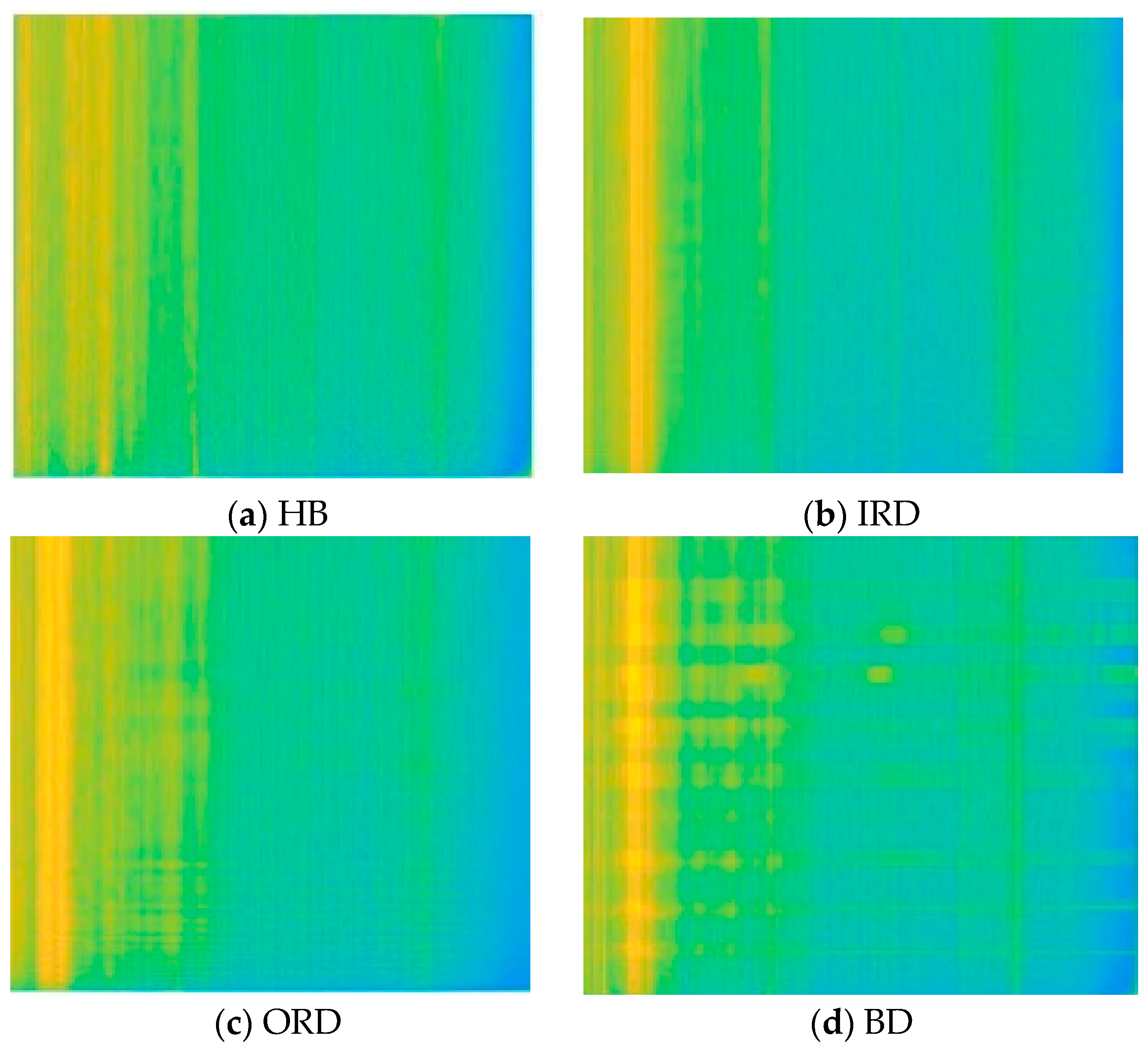
When investigating more complex techniques for diagnosing bearing faults, utilizing the Q transform is an effective way to improve the accuracy of fault detection methods. This study shows how to use different transforms on bearing fault signals in a certain order to find important features that are needed for diagnosing bearing defects. The DCT is applied to all bearing fault signals to produce a set of coefficients at the beginning of the procedure. The Q transform is then used to create a spectrogram. The basis of this spectrogram is used to extract a wide range of features, each of which offers a distinct perspective on the characterization of bearing faults. Applying the DCT to bearing fault signals results in a sequence of cosine functions that convert the time-domain data to a frequency-domain expression. The coefficients that this transformation makes show the energy concentration at different frequencies, showing patterns and irregularities that are already in the bearing signals. The Q transform is used after the DCT to turn the acquired coefficients into a spectrogram, which is a time-frequency mapping. The Q transform, a very useful tool for signal analysis, offers a multi-resolution view of the signal, enabling the identification of ephemeral elements often overlooked by other types of analysis. The method produces a spectrogram, which indicates the frequency elements of the signal visually over time, making bearing fault abnormalities easier to identify. Figure 2 shows the sample spectrogram corresponding to four bearing faults: healthy (HB), defect in the ball (BD), defect in the inner race (IRD), and defect in the outer race (ORD). Changes in color intensity and pattern distribution reveal a distinct time-frequency association in each spectrogram, suggesting the specific fault conditions. Color intensity, associated with the energy or amplitude in the signal and the spatial distribution of these intensities throughout the time-frequency plane, significantly contributes to the diagnosis details. Healthy bearing spectrograms, Figure 2a have a continuous cooler spectrum (greens and blues) with few high-intensity frequencies (yellows). The consistency in bearing operation suggests no major defects. On the other hand, as observed in Figure 2b, the spectrogram demonstrating DIR shows occasional vertical streaks of increased intensity (yellows and oranges). The presence of these recurring vertical lines indicates the specific impact frequencies caused by a defect in the inner race. The ORD is distinguished by a sequence of diagonal lines exhibiting heightened intensity, as observed in Figure 2c. The lines’ diagonal alignment serves as an indicator of the temporal variation in the magnitude of the defect’s influence on the rolling elements. The fourth spectrogram, Figure 2d represents the DB condition, exhibiting a disordered and scattered arrangement of high-intensity spots (yellows and reds). The observed unpredictability implies that when the faulty ball undergoes rotation and meets the races, it produces an uneven arrangement of vibrations with high frequencies.

Table 2. List of features extracted from spectrograms.

S. No.	Features	Details	S. No.	Features	Details
1	Max	It indicates the largest value in the given dataset.	9	Peak2Peak	It is a difference between the highest and lowest data points.
2	Median	It represents the mid-value of a given dataset.	10	Peak2Rms	It shows the difference between peaks to RMS values.
3	Average	$Average=\frac{a_1 + a_2 + a_3 + \dots a_n}{n}$	11	Root Sum of Square	It represents the summation of the squared value of data.
4	Kurtosis	$Kurtosis=\frac{{\mu }_4}{{\sigma }^4}$	12	Crest Factor	$C.F.=\frac{Peak}{RMS}$
5	Skewness	The probability distribution in a given dataset can be found by skewness.	13	Foam Factor	$F.F.=\frac{Peak to Peak}{Average}$
6	Standard Deviation	It is defined as a variation in the data concerned with an average value.	14	Shape Factor	$S.F.=\frac{RMS}{Average}$
7	Variance	$Variance=\sqrt{\frac{\sum {\left(x_i-\overline{x}\right)}^2}{N-1}}$	15	L Factor	$L.F.=\frac{Peak}{Root sum of square}$
8	Root Mean Square	${RMS}^2=\frac{\sum {x_i}^2}{n}$	16	Shannon Entropy	It measures the uncertainty in the data process.

shows the features extracted from all spectrograms corresponding to acquired vibration signals.

3. Results and Discussion

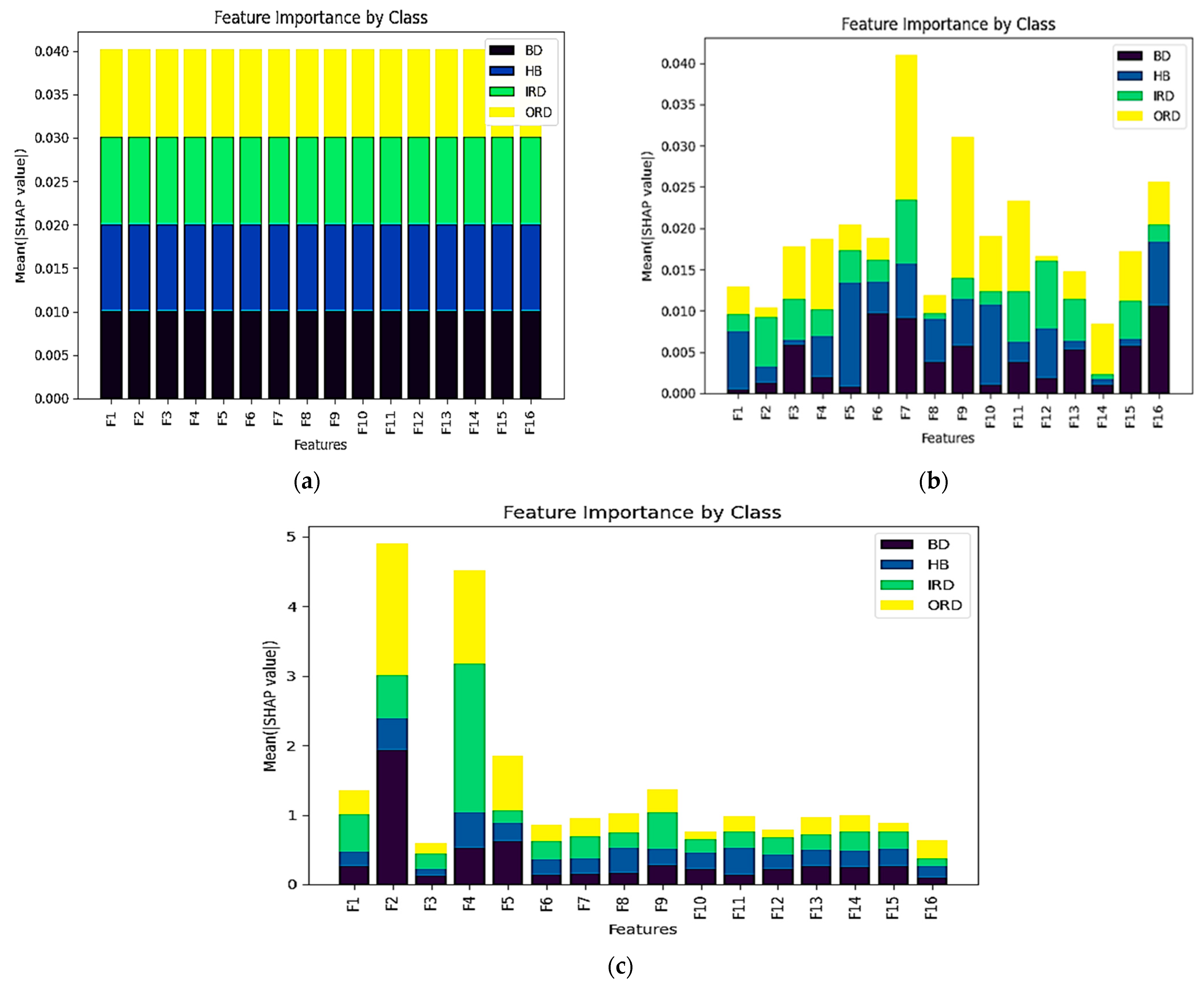
The present investigation used a hybrid methodology to diagnose faults using the CWRU-bearing dataset. The 64 vibration signals representing various fault conditions of bearing—HB, BD, IRD, and ORD—were preprocessed through the Q transform. HOG statistical features were extracted from each fault condition and ranked with the XAI. Classifiers like SVM, LSTM, and GRU are considered for the initial training of the constructed feature vectors, and in a later stage, tenfold cross-validation is performed to avoid overfitting of models. To reduce complexity and improve the diagnostic model’s performance, feature selection is essential to fault diagnosis because it helps determine the most applicable and discriminative attributes from the dataset. By identifying the most informative attributes, superfluous data can be removed, thereby lowering computational complexity and lowering the chance of overfitting, which improves diagnostic accuracy. In the present work, XAI (SHAP)-based feature selection techniques were applied to the extracted features of all four bearing fault conditions. Figure 3 shows the bar chart representing feature selection using XAI models. Figure 3a displays the feature significance graph, which displays the outcomes of using an SVM as an XAI model. The graph evaluates the relative relevance of sixteen distinct features—identified as F1 through F16—across four distinct fault classes using SHAP values. Each factor contributed substantially to the classification assessments for every fault condition, as the bar chart illustrates. The vertical axis’ SHAP values show the average influence of a feature on the result of the model, which translates to a feature’s relative significance in the SVM’s decision-making process. The graphic reveals that the features F6 through F10 appear to have the highest mean SHAP values across all fault conditions, indicating their significant influence on the model’s predictions. F1, on the other hand, has the smallest effect, as evidenced by its lowest mean SHAP value. The purple bar segments’ larger SHAP values for F9 and F10 indicate their highest significance for the BD class. Blue indicates that features F6 and F7 appear to have the greatest influence on class HB. The profile of the IRD is comparable to that of HB, with F6 and F7 being particularly significant. Last but not least, the ORD has a very uniform feature importance distribution, with a minor focus on F8 and F9. This variation in the relative relevance of features between classes could point to a complex relationship between features and fault conditions. It also shows how the model can use varied information content from the same features to distinguish between various fault conditions. Figure 3b shows the feature significance as determined by an XAI architecture using a LSTM network. The influence of each feature on the predictive power of the model is assessed, and carefully examining the bar chart reveals that certain features are very important for every fault condition. The feature F10—represented by the tallest bar—seems to have a significant impact on the model’s predictions, with the greatest mean SHAP value. Conversely, the model assigns the least weight to attributes like F1 and F15, resulting in their lowest SHAP values. One noteworthy finding is the influence of certain attributes on a particular fault condition. In the fault BD, for illustration, feature F6 has a considerable impact, while in other fault conditions, its influence is quite small. This variation in feature importance may indicate that the LSTM network can recognize and use distinct features for faulty condition differentiation. Figure 3c highlights the feature’s significance when GRU is considered as an XAI model. A more thorough examination of the graph reveals a remarkable variation in the significance of the attributes under each fault condition. For instance, F4 and F10 are extremely important compared to the others, especially for the HB class. Their significant SHAP values suggest that they play a crucial part in the GRU model’s prediction ability and may be indicative of characteristics that catch severe bearing failure conditions. As an indication of their poor individual predictive value, attributes F1, F12, and F16, on the other hand, score lower on the SHAP value scale. Remarkably, the most significant attributes, F4 and F10, are undoubtedly essential in various defect conditions, potentially serving as fundamental measures of bearing health. Their increased significance under different conditions may indicate that these features are susceptible to a wide range of faulty attributes.

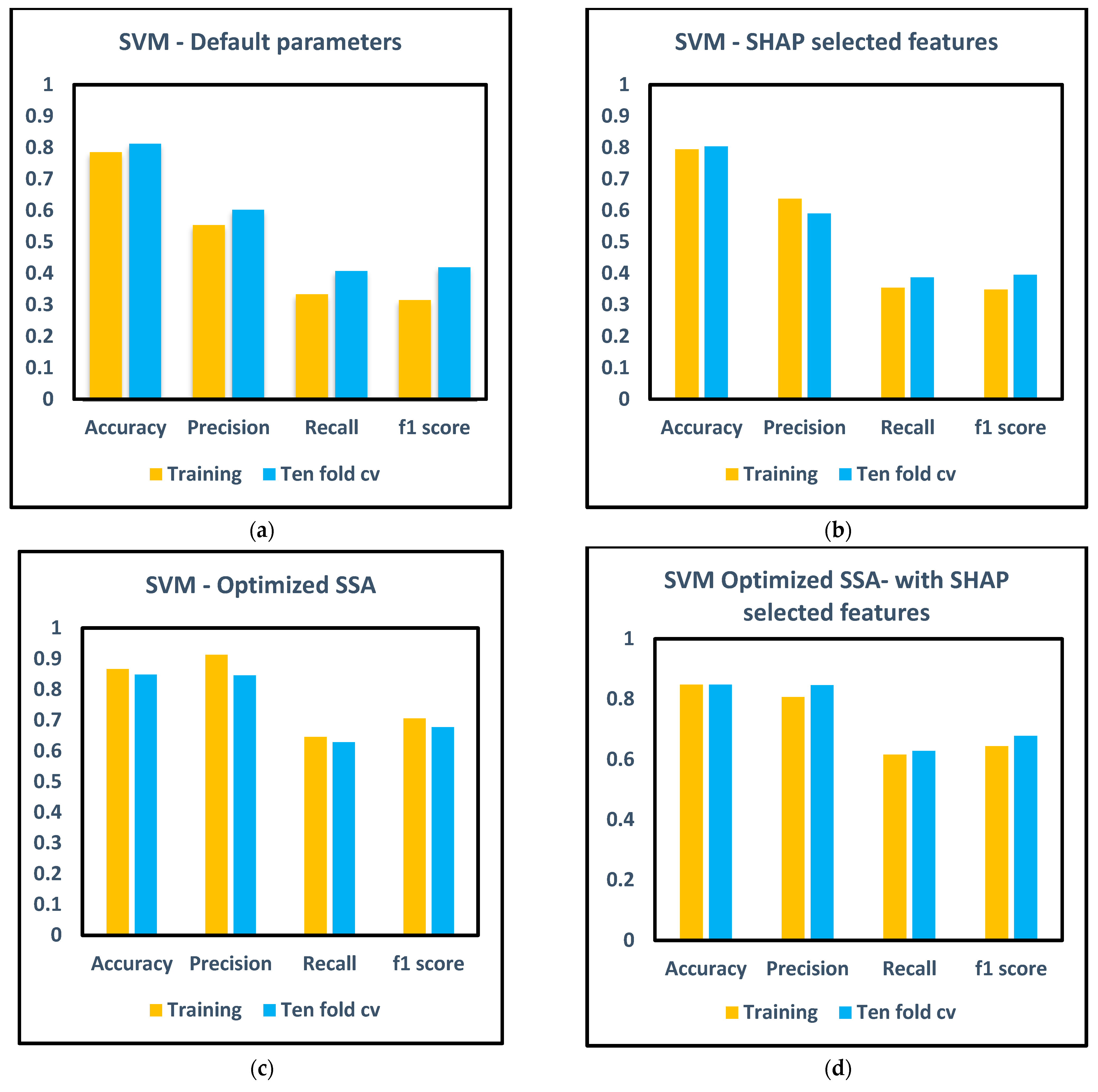
To analyze the effect of SHAP-selected features on correctly identifying various fault conditions associated with bearing, all three models were evaluated with four prediction conditions: prediction results with default hyperparameters, SHAP-selected features, SSA optimization-based hyperparameter tuning, and combined SHAP and SSA optimization. Figure 4a–d illustrate the prediction of bearing fault conditions using SVM as a prediction model. As observed in Figure 4a, the SVM model performed well when used with default parameters, achieving a training accuracy of nearly 95% and a tenfold CV accuracy of about 80%. The tenfold CV precision was close to 60%, while the precision during training was about 85%. The training recall was almost 80%, and the tenfold CV recall was 50%, whereas the training and tenfold CV F1 scores were roughly 80% and 55%, respectively. The recall and F1 score metrics showed a similar trend. The recall and F1 score metrics showed a similar trend. Figure 4b shows an apparent decrease in accuracy for all metrics when using SHAP-selected features. The SVM’s notable improvements when integrated for adjusting hyperparameters highlighted the usefulness of the SSA in improving model generalization. This was especially evident in the tenfold CV scores. The tenfold CV accuracy improved to roughly 85%, while the training accuracy stayed high at roughly 95%. Tenfold CV precision increased to 70%, while training precision grew to almost 90%. F1 scores reached 85% in training and 65% in tenfold CV, with recall rates for training and tenfold CV at 80% and 60%, respectively, as seen in Figure 4c. Combining SSA and SHAP feature selection yielded the most significant improvements, as shown in Figure 4d. With a training accuracy of 95% and a tenfold CV accuracy of 85%, the combined approach matched the results obtained with SSA optimization alone. On the other hand, during tenfold CV, the precision was marginally lower, at roughly 65%. The tenfold CV recall was at 55%, the training recall was at 75%, and the training and tenfold CV F1 scores were at 80% and 60%, respectively. Even though SSA optimization performed exceptionally well when used alone, integrating it with features chosen by SHAP did not produce better tenfold CV F1 scores. SVM prediction results are poor because identical significance across four fault conditions may indicate that features are not unique enough to increase the model’s predicted accuracy in a tenfold CV condition.

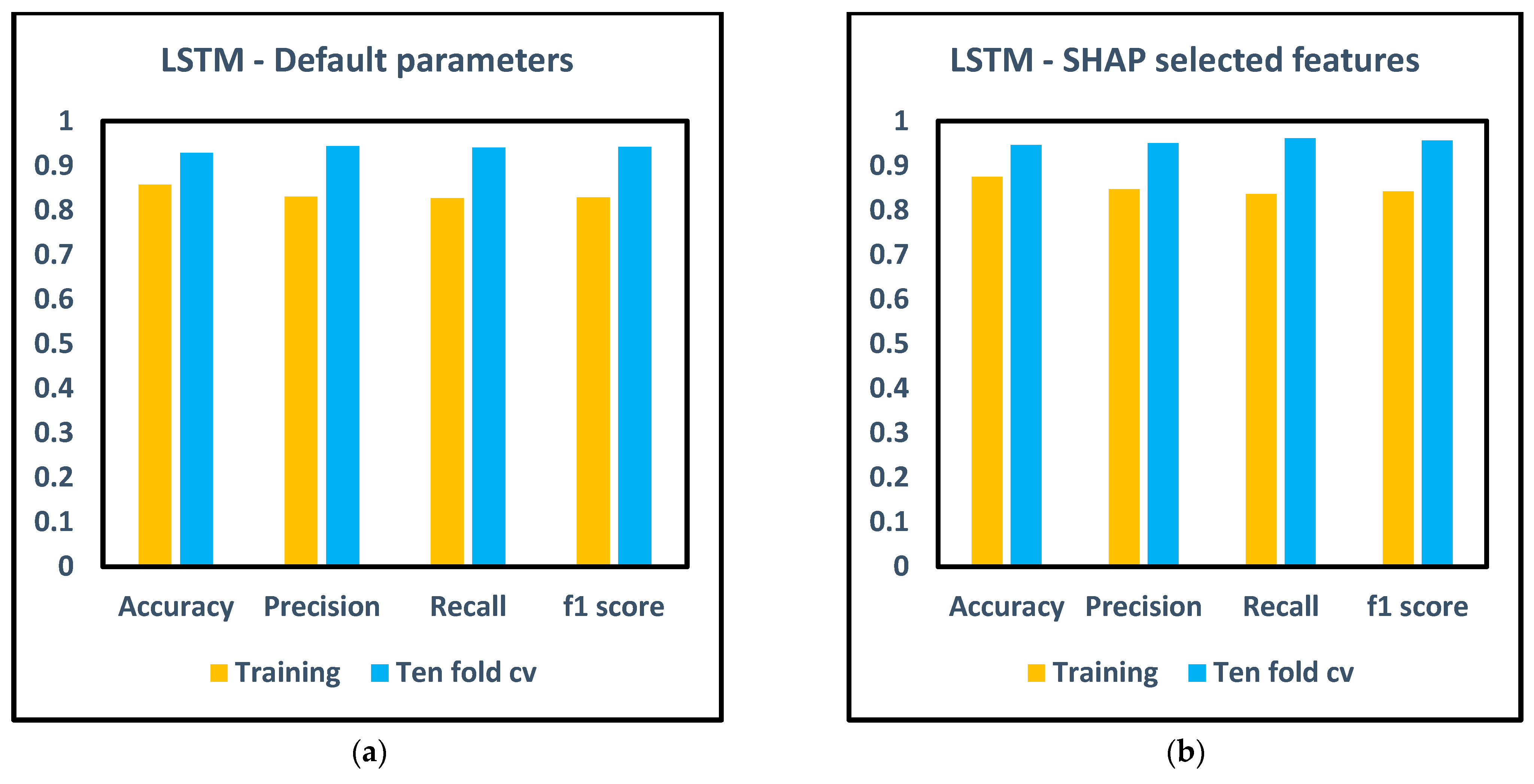
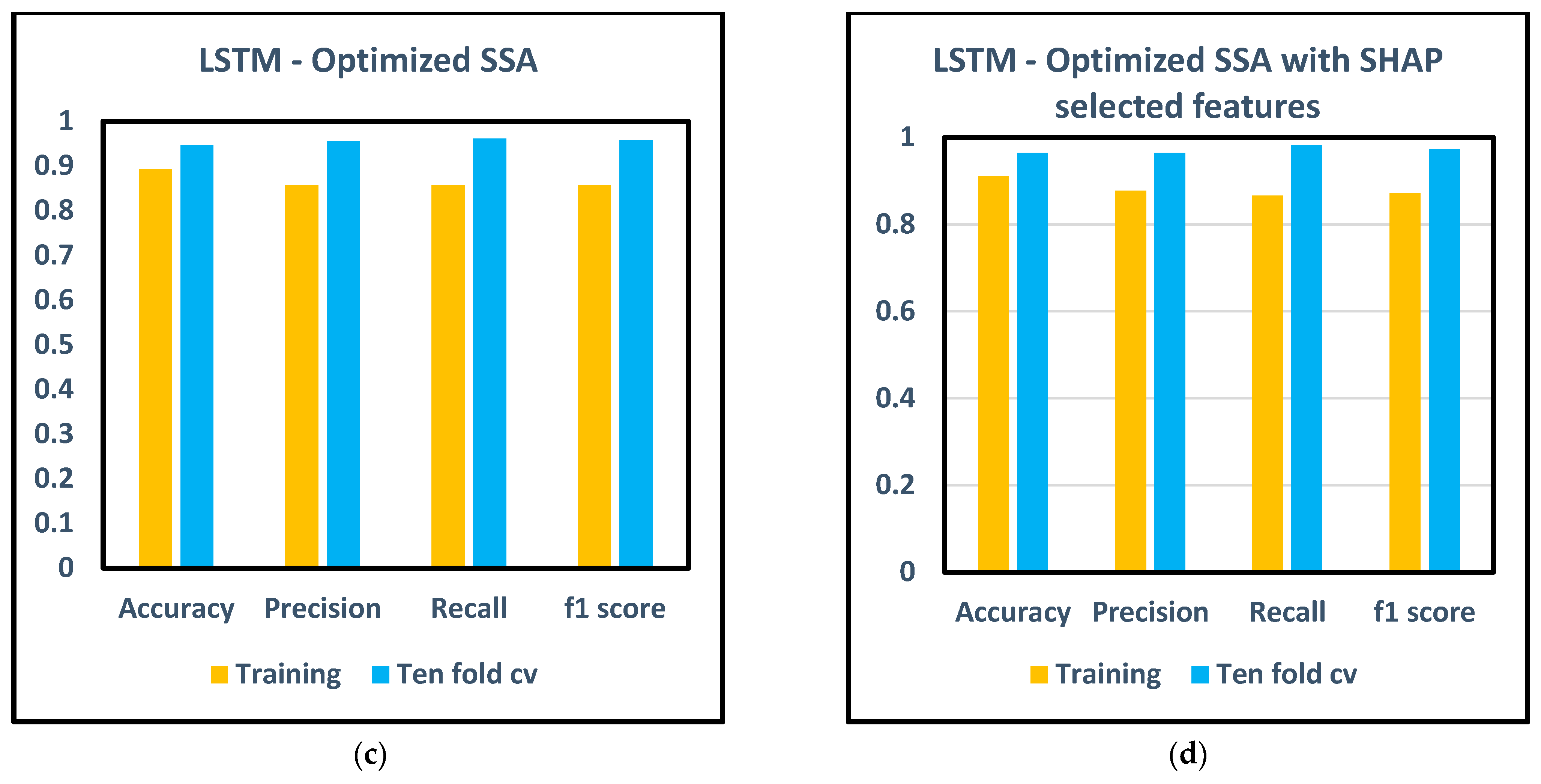
To evaluate the LSTM model’s capacity for prediction and generalizability, the assessment metrics were examined, and the prediction results can be observed in Figure 5. Effectiveness was measured using the initial configuration with default training parameters. The LSTM model achieved a training accuracy of 85.7%, and metrics such as precision, recall, and F1 score closely matched at around 0.83. The model performed significantly better when exposed to tenfold CV; accuracy increased to 92.9%, precision to 0.944, recall to 0.940, and F1 score to 0.942, as shown in Figure 5a. This improvement in the CV measures when compared to the training metrics indicates the model’s strong generalizability outside of the training dataset. After SHAP-selected features were included, an improved feature set was employed in an attempt to improve the prediction performance of the LSTM. This modification resulted in a reported training accuracy of 87.5%, and an increase in precision, recall, and F1 score to 0.847, 0.836, and 0.842, respectively (Figure 5b). The tenfold CV measures demonstrated significant improvement, reaching 94.6% for accuracy, 0.951 for precision, 0.961 for recall, and 0.956 for F1 score, indicating effective selection of the predictive features. The noteworthy increase in both recall and F1 scores during CV suggests that the model has improved its ability to accurately identify positive instances across various data folds. SSA optimization fine-tuned the LSTM’s hyperparameters, resulting in 89.3% training accuracy, a corresponding improvement in precision, recall, and F1 score, and a final score of 0.857. The tenfold CV results were identical to the configuration with SHAP-selected features, with recall at 0.961 and accuracy, precision, and F1 score at 94.6%, 0.955, and 0.958, respectively, as shown in Figure 5c. This suggests a balanced optimization of the model parameters, leading to consistent and trustworthy predictions across various data subsets. Combining SSA optimization with SHAP-selected characteristics yielded the best-predicted outcomes, as shown in Figure 5d. The training accuracy reached 91.1% with precision at 0.877, recall at 0.866, and the F1 score at 0.871. The model’s accuracy increased to 96.4% in the tenfold CV; precision also reached 0.964, recall peaked at 0.982, and the F1 score approached the optimum value of 0.973. These findings demonstrate the model’s exceptional performance in identifying and verifying genuine positive cases while preserving a high level of accuracy.

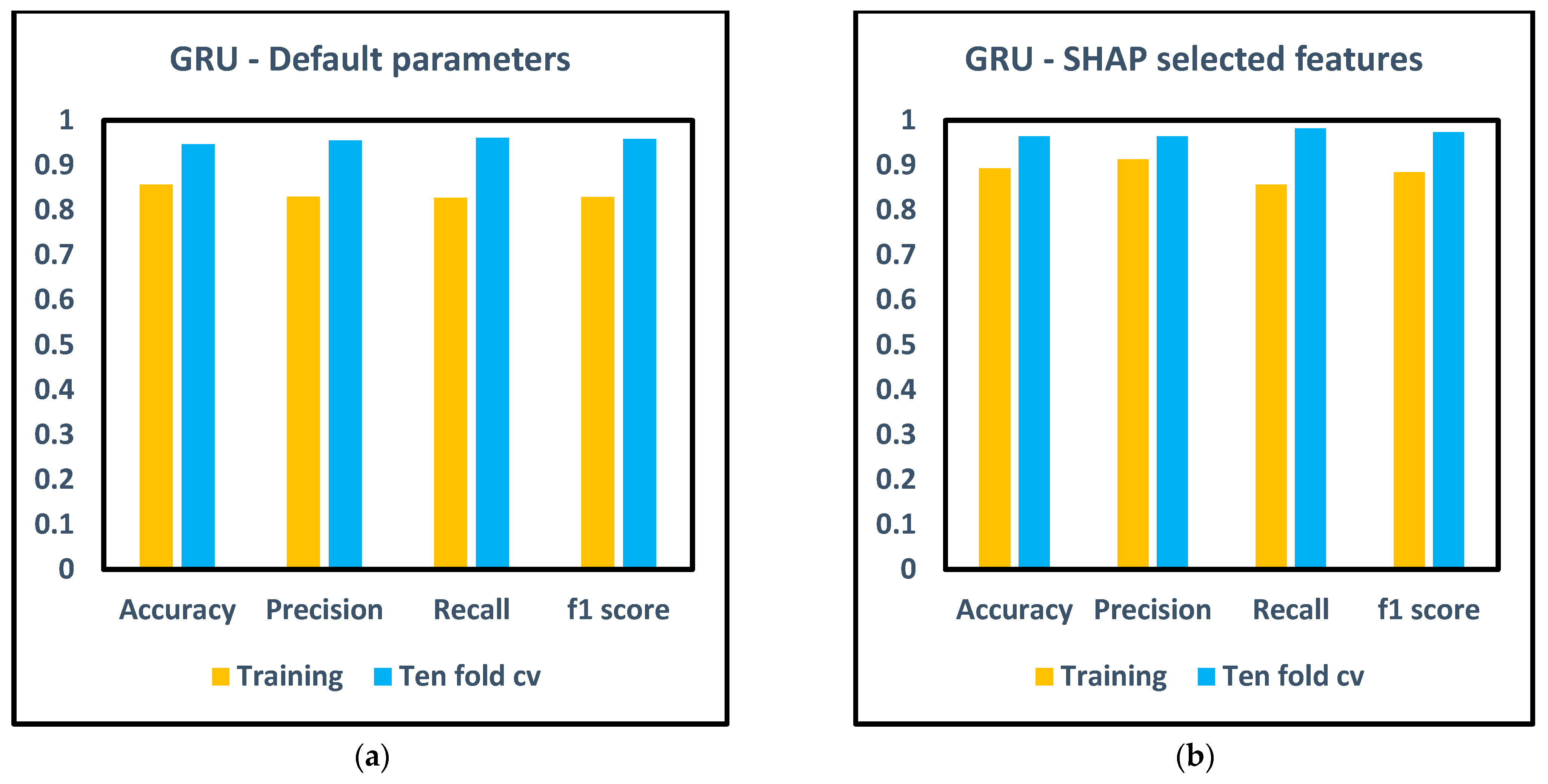
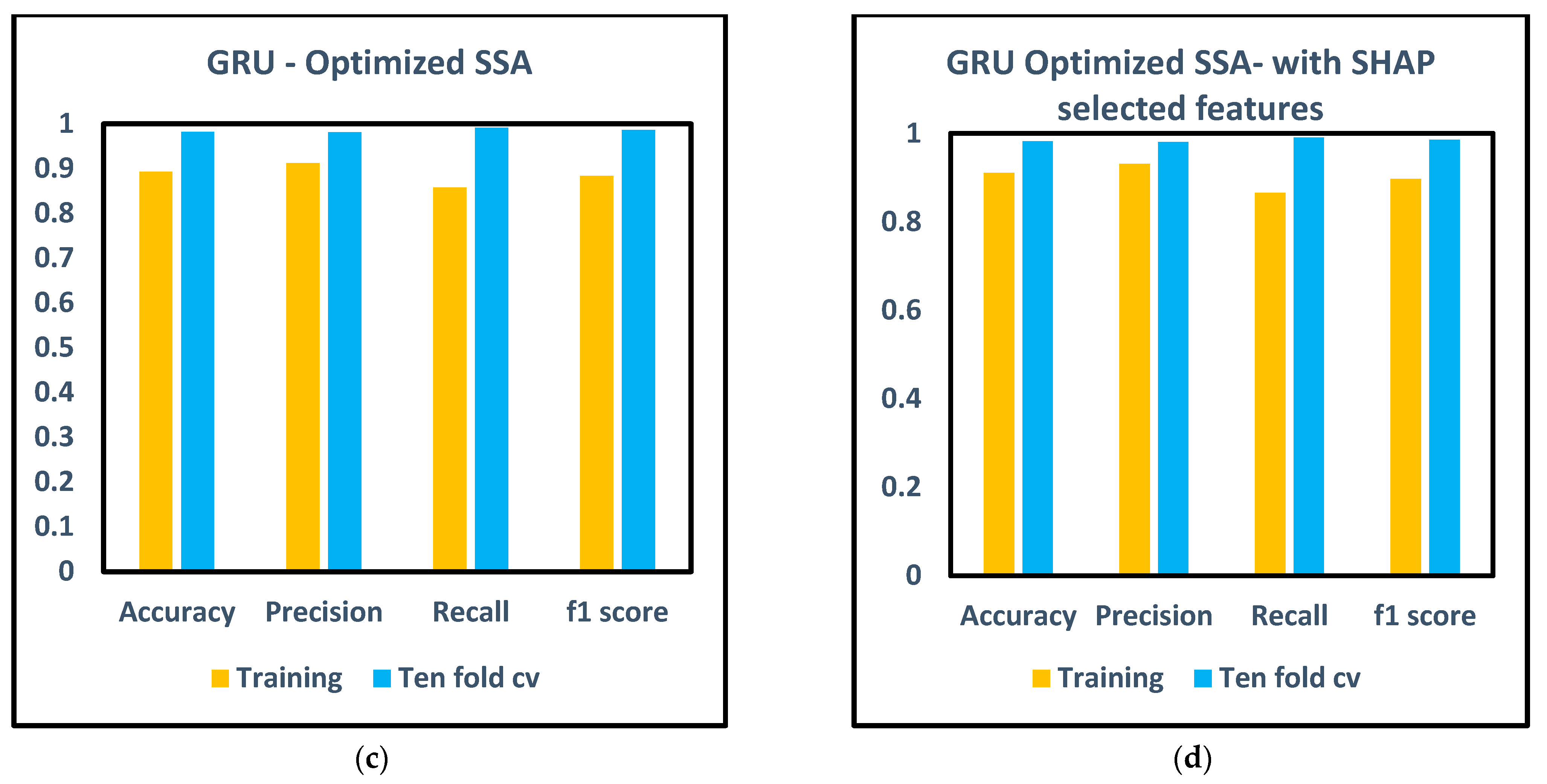
The GRU model is also assessed to diagnose bearing faults with XAI-based feature selection and metaheuristic optimization. Figure 6 presents the prediction results. With default training settings, the model achieved 85.7% training accuracy, 0.830 precision, 0.827 recall, and a 0.829 F1 score. This setup serves as a benchmark for evaluating the effectiveness of additional optimizations. Interestingly, all measures showed a considerable improvement when the model was subjected to tenfold CV; accuracy increased to 0.946, precision to 0.955, recall to 0.961, and the F1 score to 0.958, as observed in Figure 6a. These findings demonstrate the GRU model’s significant generalization ability in a more demanding and diverse testing setting. Using SHAP to choose features led to an increase in all performance parameters of the GRU model after training: accuracy reached 89.3%, precision reached 0.913, recall reached 0.857, and the F1 score reached 0.884. This improvement was also shown in the tenfold CV metrics, where accuracy was 96.4%, precision was 0.964, recall reached a high point of 0.982, and the F1 score was 0.973, highlighting the critical role that feature selection plays in enhancing model adaptability, as shown in Figure 6b. The GRU model’s hyperparameters were further optimized through testing with SSA, a novel technique influenced by the swarming patterns of salps. The resulting training measures showed 89.3% accuracy, 0.912 precision, 0.857 recall, and 0.884 F1 score, which were comparable to the SHAP-enhanced model. On the other hand, the tenfold CV showed better results: 98.2% for accuracy, 0.981 for precision, 0.991 for recall, and 0.986 for the F1 score. These figures provide compelling evidence for the effectiveness of SSA optimization in optimizing the model to obtain near-perfect recall and extraordinarily high CV precision, as observed in Figure 6c. The integration of SSA and SHAP feature selection—a strategy intended to capitalize on the advantages of both approaches—marked the achievement of the investigation’s goal. This hybrid technique produced the best training outcomes, with an F1 score of 0.898, recall of 0.866, accuracy of 91.1%, and precision of 0.931. The results of the tenfold CV were especially remarkable, with recall at an astounding 0.991 and accuracy, precision, and the F1 score all at 0.982. These numbers show that careful hyperparameter tuning combined with deliberate feature selection results in an incredibly predictive model, especially when it comes to the recall statistic, where the model performs almost perfectly, as can be observed in Figure 6d. The tenfold CV results clearly show that the hybrid technique of SHAP feature selection combined with SSA optimization leads to a GRU model with improved accuracy in diagnosis and generalization. The improvements in performance measures demonstrate the model’s improved ability to predict bearing fault conditions with high accuracy, consistency, and reliability across several data folds. Because of its high performance, the GRU model is excellent for detecting bearing faults, and it may also be used in monitoring and predictive maintenance systems across a range of industries. As the three models are compared for bearing fault diagnosis, SVM begins at a lower prediction result and does not reach the upper limits of the LSTM and GRU models, despite showing the most significant relative increase through optimization procedures. Both GRU and LSTM exhibit strong performances, with GRU outperforming LSTM by a small margin in the tenfold CV score. SSA optimization notably yields the best fault prediction results for the GRU model, demonstrating both its remarkable generalization capacity and its applicability for implementation in real-world fault diagnosis systems. As a result, even though all models gain from optimization, the GRU model—especially when SSA optimization is used—performs best in the prediction of bearing faults, providing a strong combination of accuracy and extensive detection abilities, as shown by the precision, recall, and F1 scores. This proves that GRU—optimized with SSA—is the best predictive model for diagnosing bearing faults based on the author’s proposed methodology.

The confusion matrices illustrate in

Table 3. Training and tenfold cross-validation of SVM.

Training Results (SVM)						Tenfold Cross-Validation Results (SVM)
DEFAULT	BD	HB	IRD	ORD		DEFAULT	BD	HB	IRD	ORD
BD	2	0	1	9		BD	5	0	0	7
HB	0	0	0	4		HB	0	0	0	4
IRD	0	0	2	10		IRD	0	0	3	9
ORD	0	0	0	28		ORD	1	0	0	27
(a)						(b)
SHAP	BD	HB	IRD	ORD		SHAP	BD	HB	IRD	ORD
BD	2	0	0	10		BD	4	0	0	8
HB	0	0	0	4		HB	0	0	0	4
IRD	0	0	3	9		IRD	0	0	3	9
ORD	0	0	0	28		ORD	1	0	0	27
(c)						(d)
SSA	BD	HB	IRD	ORD		SSA	BD	HB	IRD	ORD
BD	5	0	0	7		BD	6	0	0	6
HB	0	3	0	1		HB	0	3	0	1
IRD	0	0	5	7		IRD	0	0	4	8
ORD	0	0	0	28		ORD	2	0	0	26
(e)						(f)
SHAP+SSA	BD	HB	IRD	ORD		SHAP+SSA	BD	HB	IRD	ORD
BD	5	0	0	7		BD	6	0	0	6
HB	0	3	0	1		HB	0	3	0	1
IRD	0	1	4	7		IRD	0	0	4	8
ORD	1	0	0	27		ORD	2	0	0	26
(g)						(h)

a–h how well an SVM model performs when it comes to detecting bearing faults. The matrices are displayed for training and tenfold cross-validation outcomes in four experimental configurations. True positives for ORD are constantly high in the training period, indicating the SVM’s ability to detect faults. However, there are a lot of false negatives in BD and IRD detection, which suggests that it is hard to identify these particular fault conditions. Applying tenfold cross-validation noticeably increases false positives for ORD in the default parameter configuration, indicating a tendency to mistakenly identify other fault conditions as ORD. Including SHAP-selected features results in marginal gains in BD identification, despite the loss of ORD precision. SSA improves IRD identification, but raises ORD false positives. Although there is a modest increase in ORD misclassifications, the hybrid approach enhances BD and IRD identification while maintaining high true positives for ORD. This thorough examination emphasizes the importance of optimization and fine-tuning to strike a balance between sensitivity and specificity across a variety of bearing fault conditions, as well as the advantages and disadvantages of the SVM in fault classification.

Table 4. Training and tenfold cross-validation of LSTM.

Training Results (LSTM)						Tenfold Cross-Validation Results (LSTM)
DEFAULT	BD	HB	IRD	ORD		DEFAULT	BD	HB	IRD	ORD
BD	10	0	0	2		BD	11	0	0	1
HB	0	3	1	0		HB	0	4	0	0
IRD	0	1	10	1		IRD	0	0	11	1
ORD	1	0	2	25		ORD	2	0	0	26
(a)						(b)
SHAP	BD	HB	IRD	ORD		SHAP	BD	HB	IRD	ORD
BD	10	0	0	2		BD	12	0	0	0
HB	0	3	1	0		HB	0	4	0	0
IRD	0	1	10	1		IRD	0	0	11	1
ORD	1	0	1	26		ORD	1	0	1	26
(c)						(d)
SSA	BD	HB	IRD	ORD		SSA	BD	HB	IRD	ORD
BD	11	0	0	1		BD	12	0	0	0
HB	0	3	1	0		HB	0	4	0	0
IRD	0	1	10	1		IRD	0	0	11	1
ORD	1	0	1	26		ORD	2	0	0	26
(e)						(f)
SHAP+SSA	BD	HB	IRD	ORD		SHAP+SSA	BD	HB	IRD	ORD
BD	11	0	0	1		BD	12	0	0	0
HB	0	3	1	0		HB	0	4	0	0
IRD	0	1	10	1		IRD	0	0	12	0
ORD	1	0	0	27		ORD	2	0	0	26
(g)						(h)

a–h shows the confusion matrices, which are a detailed way to compare how well a LSTM network can predict things when the parameters are set to different values. The LSTM exhibits a great capacity for accurately identifying ORD across all parameter values, with remarkably high true positives, as shown in the training results matrices. It is noted that there is considerable ambiguity between BD and HB as well as between IRD and ORD when using the default settings. However, the use of both SSA and SHAP feature selection, both separately and together, significantly enhances the LSTM’s accuracy in identifying BD and IRD, as evidenced by the decrease in off-diagonal elements in the corresponding confusion matrices. This is especially true when SSA and SHAP are applied simultaneously. Across all models and parameter settings, the ORD identification is still reliable, with only a small percentage of instances incorrectly categorized as IRD or BD. These matrices show how well the LSTM finds errors and how well SHAP and SSA optimization help it make better predictions. This is especially true when the model is put through strict cross-validation tests that check if it can work with new data.

Table 5. Training and tenfold cross-validation of GRU.

Training Results (GRU)						Tenfold Cross-Validation Results (GRU)
DEFAULT	BD	HB	IRD	ORD		DEFAULT	BD	HB	IRD	ORD
BD	10	0	0	2		BD	12	0	0	0
HB	0	3	1	0		HB	0	4	0	0
IRD	0	1	10	1		IRD	0	0	11	1
ORD	1	0	2	25		ORD	2	0	0	26
(a)						(b)
SHAP	BD	HB	IRD	ORD		SHAP	BD	HB	IRD	ORD
BD	10	0	0	2		BD	12	0	0	0
HB	0	3	1	0		HB	0	4	0	0
IRD	0	1	10	1		IRD	0	0	12	0
ORD	1	0	1	26		ORD	2	0	0	26
(c)						(d)
SSA	BD	HB	IRD	ORD		SSA	BD	HB	IRD	ORD
BD	10	0	0	2		BD	12	0	0	0
HB	0	3	1	0		HB	0	4	0	0
IRD	0	0	11	1		IRD	0	0	12	0
ORD	2	0	0	26		ORD	1	0	0	27
(e)						(f)
SHAP+SSA	BD	HB	IRD	ORD		SHAP+SSA	BD	HB	IRD	ORD
BD	10	0	0	2		BD	12	0	0	0
HB	0	3	1	0		HB	0	4	0	0
IRD	0	0	11	1		IRD	0	0	12	0
ORD	1	0	0	27		ORD	1	0	0	27
(g)						(h)

a–h presents the confusion matrices, which illustrate the prediction output of the GRU model in identifying bearing fault conditions. When SHAP-selected features and SSA are integrated, either separately or in combination, the default parameter configuration shows some misclassifications between BD and HB and IRD and ORD, which are noticeably improved. These improvements result in fewer false negatives and better diagnosis of BD and IRD defects. The GRU network, especially when improved with SHAP and SSA, shows remarkable performance in the tenfold cross-validation results, with perfect identification for BD and a significant increase in identification accuracy for IRD and ORD.

4. Conclusions

The present study aims to present a methodology based on HOG features extracted from Q transform to identify bearing faults with a small sample and using deep learning models like LSTM and GRU, along with SVM. To determine the accuracy of each model’s fault detection abilities, the research uses a rigorous approach that involves training and cross-validating each model. This work employs an XAI framework, based on SHAP, to pinpoint crucial features that significantly influence the models’ predictive capabilities. The study results are systematically analyzed and assessed under four conditions: the default configuration of models, the addition of features chosen by SHAP, the optimization of hyperparameters using the SSA algorithm, and a hybrid strategy that combines SSA and SHAP. The combination of SSA optimization and SHAP significantly enhances training and tenfold cross-validation accuracy for all machine learning models under investigation.

It is noteworthy to mention that the GRU model performs better, achieving an impressive accuracy of 98.2%, particularly when enhanced by XAI-informed features and SSA optimization. The LSTM model, which has an impressive accuracy of 96.4%, comes next. Although the hybrid optimization technique shows progress, the SVM achieves a slightly lower peak accuracy of 84.82% in tenfold cross-validation. The research essentially suggests that the most effective model for fault prediction is the GRU model, which has been fitted with the attributes chosen by XAI, followed by LSTM, and finally SVM. The suggested methodological framework’s adaptability and robustness are additionally emphasized, indicating that it may be used to predict the life expectancy and performance of a variety of other mechanical systems, including motors, gearboxes, and turbine blades. The presented study succinctly conveys the important advancements in bearing problem identification and the wider implications for predictive maintenance technologies.

References

1. Li, J.; Shen, C.; Kong, L.; Wang, D.; Xia, M.; Zhu, Z. A New Adversarial Domain Generalization Network Based on Class Boundary Feature Detection for Bearing Fault Diagnosis. IEEE Trans. Instrum. Meas. 2022, 71, 2506909. [Google Scholar] [CrossRef]
2. Vakharia, V.; Kiran, M.B.; Dave, N.J.; Kagathara, U. Feature Extraction and Classification of Machined Component Texture Images Using Wavelet and Artificial Intelligence Techniques. In Proceedings of the 2017 8th International Conference on Mechanical and Aerospace Engineering (ICMAE), Prague, Czech Republic, 22–25 July 2017; pp. 140–144. [Google Scholar] [CrossRef]
3. Liu, T.C.; Wu, T.Y. Application of Empirical Mode Decomposition and Envelope Analysis to Fault Diagnosis in Roller Bearing with Single/Double Defect. Smart Sci. 2017, 5, 150–159. [Google Scholar] [CrossRef]
4. Shah, M.; Borade, H.; Sanghavi, V.; Purohit, A.; Wankhede, V.; Vakharia, V. Enhancing Tool Wear Prediction Accuracy Using Walsh–Hadamard Transform, DCGAN and Dragonfly Algorithm-Based Feature Selection. Sensors 2023, 23, 3833. [Google Scholar] [CrossRef]
5. Wang, D.; Guo, W.; Wang, X. A joint sparse wavelet coefficient extraction and adaptive noise reduction method in recovery of weak bearing fault features from a multi-component signal mixture. Appl. Soft Comput. 2013, 13, 4097–4104. [Google Scholar] [CrossRef]
6. Łuczak, D. Machine Fault Diagnosis through Vibration Analysis: Continuous Wavelet Transform with Complex Morlet Wavelet and Time–Frequency RGB Image Recognition via Convolutional Neural Network. Electronics 2024, 13, 452. [Google Scholar] [CrossRef]
7. Kumar, A.; Berrouche, Y.; Zimroz, R.; Vashishtha, G.; Chauhan, S.; Gandhi, C.P.; Xiang, J. Non-parametric Ensemble Empirical Mode Decomposition for extracting weak features to identify bearing defects. Measurement 2023, 211, 112615. [Google Scholar] [CrossRef]
8. Zhu, H.; He, Z.; Wei, J.; Wang, J.; Zhou, H. Bearing fault feature extraction and fault diagnosis method based on feature fusion. Sensors 2021, 21, 2524. [Google Scholar] [CrossRef] [PubMed]
9. Li, J.; Wang, Y.; Zi, Y.; Jiang, S. A local weighted multi-instance multilabel network for fault diagnosis of rolling bearings using encoder signal. IEEE Trans. Instrum. Meas. 2020, 69, 8580–8589. [Google Scholar] [CrossRef]
10. Zhao, D.; Li, J.; Cheng, W.; Wen, W. Bearing Multi-Fault Diagnosis with Iterative Generalized Demodulation Guided by Enhanced Rotational Frequency Matching under Time-Varying Speed Conditions. ISA Trans. 2023, 133, 518–528. [Google Scholar] [CrossRef]
11. Zhao, D.; Cai, W.; Cui, L. Adaptive Thresholding and Coordinate Attention-Based Tree-Inspired Network for Aero-Engine Bearing Health Monitoring under Strong Noise. Adv. Eng. Inform. 2024, 61, 102559. [Google Scholar] [CrossRef]
12. Zhao, D.; Wang, H.; Cui, L. Frequency-Chirprate Synchrosqueezing-Based Scaling Chirplet Transform for Wind Turbine Nonstationary Fault Feature Time–Frequency Representation. Mech. Syst. Signal Process. 2024, 209, 111112. [Google Scholar] [CrossRef]
13. Kiakojouri, A.; Lu, Z.; Mirring, P.; Powrie, H.; Wang, L. A Novel Hybrid Technique Combining Improved Cepstrum Pre-Whitening and High-Pass Filtering for Effective Bearing Fault Diagnosis Using Vibration Data. Sensors 2023, 23, 9048. [Google Scholar] [CrossRef] [PubMed]
14. Hoang, D.T.; Tran, X.T.; Van, M.; Kang, H.J. A Deep Neural Network-Based Feature Fusion for Bearing Fault Diagnosis. Sensors 2021, 21, 244. [Google Scholar] [CrossRef]
15. Sugumaran, V.; Jain, D.; Amarnath, M.; Kumar, H. Fault Diagnosis of Helical Gear Box Using Decision Tree Through Vibration Signals. Int. J. Perform. Eng. 2013, 9, 221–234. [Google Scholar] [CrossRef]
16. Vakharia, V.; Gupta, V.K.; Kankar, P.K. A Comparison of Feature Ranking Techniques for Fault Diagnosis of Ball Bearing. Soft Comput. 2016, 20, 1601–1619. [Google Scholar] [CrossRef]
17. Pham, M.T.; Kim, J.M.; Kim, C.H. Deep learning-based bearing fault diagnosis method for embedded systems. Sensors 2020, 20, 6886. [Google Scholar] [CrossRef]
18. Yang, K.; Zhao, L.; Wang, C. A new intelligent bearing fault diagnosis model based on triplet network and SVM. Sci. Rep. 2022, 12, 5234. [Google Scholar] [CrossRef]
19. Li, B.; Zhang, P.L.; Tian, H.; Mi, S.S.; Liu, D.S.; Ren, G.Q. A new feature extraction and selection scheme for hybrid fault diagnosis of gearbox. Expert Syst. Appl. 2011, 38, 10000–10009. [Google Scholar] [CrossRef]
20. Karabadji, N.E.I.; Seridi, H.; Khelf, I.; Azizi, N.; Boulkroune, R. Improved decision tree construction based on attribute selection and data sampling for fault diagnosis in rotating machines. Eng. Appl. Artif. Intell. 2014, 35, 71–83. [Google Scholar] [CrossRef]
21. Rajeswari, C.; Sathiyabhama, B.; Devendiran, S.; Manivannan, K. A gear fault identification using wavelet transform, rough set based GA, ANN and C4. 5 algorithm. Procedia Eng. 2014, 97, 1831–1841. [Google Scholar] [CrossRef]
22. Gao, K.; Wu, Z.; Yu, C.; Li, M.; Liu, S. Composite Fault Diagnosis of Rolling Bearings: A Feature Selection Approach Based on the Causal Feature Network. Appl. Sci. 2023, 13, 9089. [Google Scholar] [CrossRef]
23. Harinarayan, R.R.A.; Shalinie, S.M. XFDDC: eXplainable Fault Detection Diagnosis and Correction framework for chemical process systems. Process Saf. Environ. Prot. 2022, 165, 463–474. [Google Scholar] [CrossRef]
24. Meas, M.; Machlev, R.; Kose, A.; Tepljakov, A.; Loo, L.; Levron, Y.; Belikov, J. Explainability and transparency of classifiers for air-handling unit faults using explainable artificial intelligence (XAI). Sensors 2022, 22, 6338. [Google Scholar] [CrossRef]
25. Rashidi, S.; Fallah, A.; Towhidkhah, F. Feature extraction based DCT on dynamic signature verification. Sci. Iran. 2012, 19, 1810–1819. [Google Scholar] [CrossRef]
26. Pang, Y.; Jia, L.; Liu, Z. Discrete cosine transformation and temporal adjacent convolutional neural network-based remaining useful life estimation of bearings. Shock Vib. 2020, 2020, 8240168. [Google Scholar] [CrossRef]
27. Madhu, C.; Shankar, E.A.; Reddy, N.S.; Srinivasulu, D. Signal estimation reproduction in frequency domain using tunable Q-factor wavelet transform. In Proceedings of the Second International Conference on Emerging Trends in Science Technologies for Engineering Systems (ICETSE-2019), Karnataka, India, 17–18 May 2019; Elsevier: Amsterdam, The Netherlands, 2019. [Google Scholar] [CrossRef]
28. Zhou, W.; Gao, S.; Zhang, L.; Lou, X. Histogram of oriented gradients feature extraction from raw bayer pattern images. IEEE Trans. Circuits Syst. II Express Briefs 2020, 67, 946–950. [Google Scholar] [CrossRef]
29. Vakharia, V.; Shah, M.; Suthar, V.; Patel, V.K.; Solanki, A. Hybrid perovskites thin films morphology identification by adapting multiscale-SinGAN architecture, heat transfer search optimized feature selection and machine learning algorithms. Phys. Scr. 2023, 98, 025203. [Google Scholar] [CrossRef]
30. Almalki, Y.E.; Ali, M.U.; Ahmed, W.; Kallu, K.D.; Zafar, A.; Alduraibi, S.K.; Irfan, M.; Basha, M.A.A.; Alshamrani, H.A.; Alduraibi, A.K. Robust Gaussian and Nonlinear Hybrid Invariant Clustered Features Aided Approach for Speeded Brain Tumor Diagnosis. Life 2022, 12, 1084. [Google Scholar] [CrossRef]
31. Wang, M.; Chen, Y.; Zhang, X.; Chau, T.K.; Ching Iu, H.H.; Fernando, T.; Ma, M. Roller bearing fault diagnosis based on integrated fault feature and SVM. J. Vib. Eng. Technol. 2021, 10, 853–862. [Google Scholar] [CrossRef]
32. Tian, H.; Fan, H.; Feng, M.; Cao, R.; Li, D. Fault diagnosis of rolling bearing based on hpso algorithm optimized cnn-lstm neural network. Sensors 2023, 23, 6508. [Google Scholar] [CrossRef] [PubMed]
33. Wu, G.; Ning, X.; Hou, L.; He, F.; Zhang, H.; Shankar, A. Three-dimensional Softmax Mechanism Guided Bidirectional GRU Networks for Hyperspectral Remote Sensing Image Classification. Signal Process. 2023, 212, 109151. [Google Scholar] [CrossRef]
34. Brito, L.C.; Susto, G.A.; Brito, J.N.; Duarte, M.A. An explainable artificial intelligence approach for unsupervised fault detection and diagnosis in rotating machinery. Mech. Syst. Signal Process. 2022, 163, 108105. [Google Scholar] [CrossRef]
35. Chen, H.Y.; Lee, C.H. Vibration signals analysis by explainable artificial intelligence (XAI) approach: Application on bearing faults diagnosis. IEEE Access 2020, 8, 134246–134256. [Google Scholar] [CrossRef]
36. Brusa, E.; Cibrario, L.; Delprete, C.; Di Maggio, L.G. Explainable AI for machine fault diagnosis: Understanding features’ contribution in machine learning models for industrial condition monitoring. Appl. Sci. 2023, 13, 2038. [Google Scholar] [CrossRef]
37. Loparo, K.A. Case Western Reserve University Dataset. Bearing Data Centre. Available online: https://engineering.case.edu/bearingdatacenter (accessed on 10 January 2024).
Figure 1. Proposed framework for fault diagnosis using machine learning model.
Machines 12 00373 g001
Figure 2. Sample spectrogram of four bearing conditions.
Machines 12 00373 g002
Figure 3. Feature selection plot using XAI: (a) SVM, (b) LSTM, and (c) GRU.
Machines 12 00373 g003
Figure 4. Training and tenfold cross-validation for SVM: (a) default parameters, (b) SHAP-selected features, (c) SSA optimization, (d) combination of SHAP and salp.
Machines 12 00373 g004
Figure 5. Training and tenfold cross-validation for LSTM: (a) default parameters, (b) SHAP-selected features, (c) SSA optimization, (d) combination of SHAP and salp.
Machines 12 00373 g005aMachines 12 00373 g005b
Figure 6. Training and tenfold cross-validation for GRU: (a) default parameters, (b) SHAP-selected features, (c) SSA optimization, (d) combination of SHAP and salp.
Machines 12 00373 g006aMachines 12 00373 g006b