Fuzzy-Based Image Contrast Enhancement for Wind Turbine Detection: A Case Study Using Visual Geometry Group Model 19, Xception, and Support Vector Machines

Abstract

Traditionally, condition monitoring of wind turbines has been performed manually by certified rope teams. This method of inspection can be dangerous for the personnel involved, and the resulting downtime can be expensive. Wind turbine inspection can be performed using autonomous drones to achieve lower downtime, cost, and health risks. To enable autonomy, the field of drone path planning can be assisted by this research, namely machine learning that detects wind turbines present in aerial RGB images taken by the drone before performing the maneuvering for turbine inspection. For this task, the effectiveness of two deep learning architectures is evaluated in this paper both without and with a proposed fuzzy contrast enhancement (FCE) image preprocessing algorithm. Efforts are focused on two convolutional neural network (CNN) variants: VGG19 and Xception. A more traditional approach involving support vector machines (SVM) is also included to contrast a machine learning approach with our deep learning networks. The authors created a novel dataset of 4500 RGB images of size $210\times 210$ to train and evaluate the performance of these networks on wind turbine detection. The dataset is captured in an environment mimicking that of a wind turbine farm, and consists of two classes of images: with and without a small-scale wind turbine (12V Primus Air Max) assembled at Utah Valley University. The images were used to describe in detail the analysis and implementation of the VGG19, Xception, and SVM algorithms using different optimization, model training, and hyperparameter tuning technologies. The performances of these three algorithms are compared in depth alongside those augmented using the proposed FCE image preprocessing technique.

1. Introduction

In recent years, the demand for renewable energy generated from wind power has increased rapidly. The year 2021 reflects this as wind’s second-best year of growth despite pandemic conditions disrupting the industry and introducing supply chain problems [1].

Wind turbines used to harness wind power can be damaged and degraded by their environments [2,3,4,5]. When the blades of wind turbines fail, the effects can be disruptive by leading to a long-term shutdown of operations. Wind turbine blades were found to cause over 5% of wind turbine failures in a study that surveyed more than 1500 wind turbines for fifteen years [6]. These failures can result in wind turbine downtime over ten days [7]. Continuous condition monitoring of wind turbines can remediate such issues before a wind turbine failure occurs.

Traditionally, rope teams manually inspect wind turbines for possible damages such as cracks on the blades [8]. This includes certified professionals from organizations such as the Industrial Rope Access Trade Association (IRATA) and the Society of Professional Rope Access Technicians (SPRAT) [9,10]. However, conditions surrounding wind turbines could be dangerous to personnel, providing hurdles for wind energy maintenance, and potentially increasing the cost. Additionally, in-person inspection requires turbine shutdown, resulting in higher downtime. Consequently, alternative methods of inspecting wind turbines are of great interest: the market is quickly turning towards unmanned aerial vehicles (UAVs) and drones for inspecting wind turbines [8,11]. Organizations such as Clobotics and Arthwind are pioneering work in this field [12,13]. Similar interest is seen in academia [14,15,16,17]. One issue that still needs to be solved with the adoption of drone inspection is presenting the data acquired from drones in a way that is understandable to the engineers performing maintenance [11]. To mitigate this problem, a system needs to be developed to allow the drones to act autonomously and preferably respond with a single output indicating whether a wind turbine requires maintenance or not.

An initial key aspect of this type of autonomous drone inspection is its ability to accurately identify the presence of wind turbines in the field. Machine learning has been proven to be a powerful tool for classifying objects in images [18]. A classical approach to machine learning involves the use of support vector machines (SVMs). Convolutional neural networks (CNNs) are also extensions of the branch of machine learning known as neural networks (NNs), and are particularly adept at classifying images, making them instrumental to the task of identifying wind turbines [19,20].

Similar to NNs, CNNs are composed of node layers acting as a linear regression model followed by a nonlinear activation function that prevents them from collapsing into a single linear model and allows the network to represent more complicated relationships. CNNs are composed primarily of three node layers: convolutional layers, pooling layers, and fully connected (FC) layers.

In an effort to improve the performance of autonomous wind turbine inspection, this paper analyzes and compares the effects of applying fuzzy contrast enhancement (FCE) to three machine learning methods trained on the preliminary stage of wind turbine inspection: classifying whether RGB images contain wind turbines. If FCE successfully improves the performance of wind turbine detection, it may be evaluated in future research to improve the performance of other stages of wind turbine inspection as well, such as through the enhancement of defects in images of wind turbine blades. Fuzzification is used in an attempt to make the wind turbines more noticeable in the RGB aerial images via FCE preprocessing. This can potentially be manipulated to further increase accuracy in all the tested machine learning methods. The machine learning algorithms explored are the visual geometry group model 19 (VGG19), Xception, and SVM. The VGG19 and Xception architectures were selected to represent the state of the art for evaluation of FCE. SVM is a lightweight machine learning approach; it was selected to evaluate the performance of FCE on an algorithm that requires fewer computational resources. To our knowledge, FCE has not been applied to Xception previously. It has been applied to VGG16, a precursor to VGG19 [21,22]. However, we found no instances where it has been applied to VGG19 through our research. FCE has previously been applied to SVM, so the performance of this algorithm is included here as a baseline for comparison with the VGG19 and Xception deep learning algorithms [21].

An overview of our approach to training and testing the machine learning (ML) algorithms adopted in this study is summarized in Figure 1. A dataset of 4500 aerial RGB images was captured by a DJI Matrice 300 RTK drone with Zenmuse L1 RGB camera at Utah Valley University (UVU). The images were used to train the three network architectures: the SVM machine learning approach and the VGG19 and Xception deep learning approaches. The hyperparameters within these networks were tuned, and the effects of applying the proposed FCE algorithm were explored by implementing fifteen case studies: A1–A5, B1–B6, and C1–C4. For each architecture, the first corresponding case studies found the set of hyperparameters that performed best for that architecture. Afterwards, the proposed FCE was applied to each architecture tuned with the corresponding best performing set of hyperparameters. The best results from each network architecture were then compared to determine the most suitable method for wind turbine recognition in RGB images. The main contributions of this paper are as follows:

• Implementation of the proposed fuzzy contrast enhancement (FCE) image preprocessing step for VGG19, Xception and SVM algorithms. Additionally, the performances of all algorithms without and with the proposed FCE were analyzed and compared.
• Creation of a novel RGB dataset of 4500 aerial images from a Primus Air Max small wind turbine mimicking the environment of a wind turbine farm using a small-scale wind turbine prototype to compare the performance of the three ML algorithms.
• Detailed analyses and implementation of the VGG19, Xception, and SVM algorithms using different optimization methods, model training, and hyperparameter tuning technologies.

The remainder of this paper is organized as follows: The architectures of the VGG19, Xception, and SVM networks are described in Section 2 and Section 3. The fuzzy contrast enhancement is detailed in Section 4. The formulation and process of hyperparameter tuning, including categories, batch size, loss function, and dropout, are presented in Section 5. The generated dataset of 4500 RGB images and experimental results of the fifteen case studies are presented in Section 6. The last section summarizes the findings, followed by suggestions for future work.

2. Convolutional Neural Networks (CNNs)

CNNs are a type of neural network that is particularly well-suited for image classification and recognition tasks. They are composed of one or more convolutional layers, which perform the convolution operation on the input data. An example of this transformation is shown in Figure 2. In this operation, a kernel is slid along the input layer, computing the elementwise product between the kernel and each portion of the input layer. The sum of these products is then arranged in a new 2-D array of weights known as the feature map, which is the output of the convolution layer [20].

CNNs use pooling layers to reduce the size of the input data. This reduces the complexity and increases the efficiency of the neural network. Another feature commonly used in CNNs is the fully connected (FC) layer. As the name suggests, this layer maps every input node to every output node. The final layer in a CNN is typically an FC layer, as this layer can make connections between all of the data at the end of the network and the final network output. This enables the final nodes in the CNN to contain the likelihood that the input image belongs to each class [19]. The CNN architectures used in this research, both VGG19 and Xception, were created and trained using the Keras software package available for the Python programming language [23].

2.1. VGG19

One of the architectures explored in this paper focuses on transfer learning built on a VGG network, a fundamental yet renowned machine learning algorithm introduced by Andrew Zisserman and Karen Simonyan [24]. In order to maneuver large-scale pictures, the VGG model analyzes the depth of layers using a relatively small convolutional filter size $(3\times 3)$ [25]. The pretrained visual geometry group model 19 (VGG19) was trained on the ImageNet database of more than a million images from 1000 classes. All database images were RGB of size $224\times 224$ pixels [26].

The first 16 layers of VGG19 are convolution layers and the last 3 layers are dense (fully connected) layers [26]. Five blocks of convolution are present in VGG19. Each block goes along with one MaxPool Layer. Block 1: The depth of filters is 64 with two convolution layers. Block 2: The depth of filters is 128, with two convolution layers. Block 3: The depth of filters is 256, with four convolution layers. Block 4 and Block 5: The depth of filters is 512, with four convolution layers [27]. The architecture of the model is summarized in detail in

Table 1. VGG19 layer architecture.

Layer #	Layer Details	Layer #	Layer Details
1	Conv$3\times 3$ (64)	11	Conv$3\times 3$ (512)
2	Conv$3\times 3$ (64)	12	Conv$3\times 3$ (512)
-	MaxPool	-	MaxPool
3	Conv$3\times 3$ (128)	13	Conv$3\times 3$ (512)
4	Conv$3\times 3$ (128)	14	Conv$3\times 3$ (512)
-	MaxPool	15	Conv$3\times 3$ (512)
5	Conv$3\times 3$ (256)	16	Conv$3\times 3$ (512)
6	Conv$3\times 3$ (256)	-	MaxPool
7	Conv$3\times 3$ (256)	17	Fully Connected (4096)
8	Conv$3\times 3$ (256)	18	Fully Connected (4096)
-	MaxPool	19	Fully Connected (1000)
9	Conv$3\times 3$ (512)	-	SoftMax
10	Conv$3\times 3$ (512)	-	-

.

There are three potential approaches for the application of transfer learning on VGG19. The first approach runs the convolution base on an image dataset, recording its output to a Numpy array on the disk storage and then using this data as input to a densely-connected classifier. This solution is fast and computationally inexpensive to execute as it only requires running the convolution base once for each input image. The second approach runs the whole model front-to-end every time the image passes through the convolution base prior to reaching the dense layer. This increases accuracy at the cost of speed. This is the most widely used approach since it balances between the model performance and speed. The third approach is fine-tuning, which consists of unfreezing a few of the top layers of a model base used for feature extraction and simultaneously training both the fully connected classifier and these top layers. This method is computationally costly but suitable when the training images are quite different from the those in the ImageNet database [27].

VGG19 is useful because it is a CNN with an uncomplicated structure that is effective at image classification. It is therefore suitable for wind turbine classification, and this paper includes an emphasis on the VGG19 model as one of the three methods to classify wind turbines in the RGB image dataset created at UVU and to evaluate the FCE algorithm.

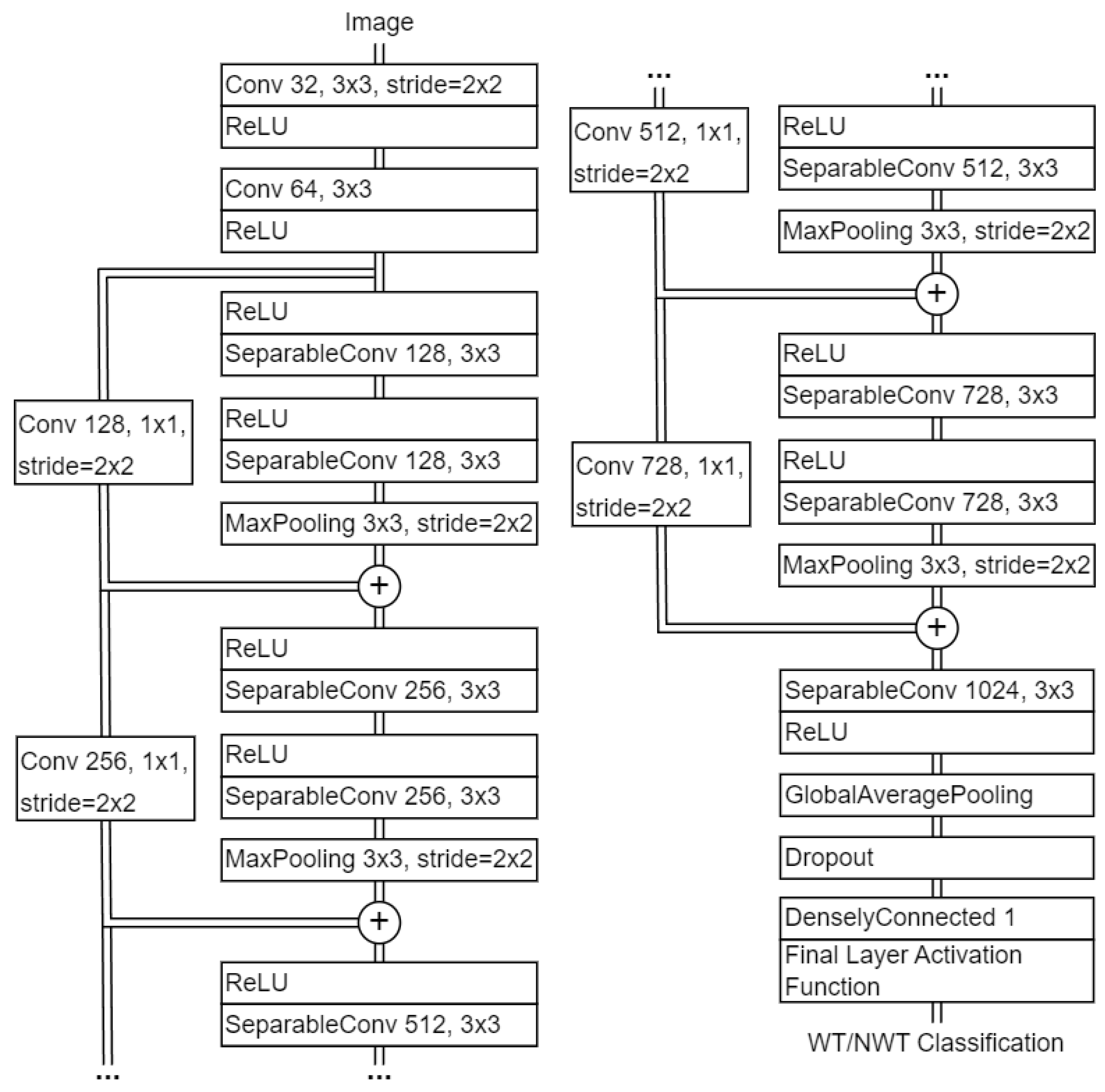
2.2. Xception

The Xception architecture is a CNN evolved from Inception, a similar class of CNN originally presented in [28]. The first variant of Inception, Inception-v1, replaces the traditional convolution layer with the Inception module, a collection of multiple convolution operations of varying kernel sizes. The Inception architecture was subsequently refined (Inception-v2) and followed by Inception-v3. Inception-v2 integrates batch normalization within the model’s architecture [29]. Inception-v3 modifies the convolution kernel to increase the architecture’s computational efficiency [30].

In [31], the author recognized that the Inception module factors the traditional CNN convolution layer into components that separately perform spatial and cross-channel correlations. Therefore, they presented the hypothesis that spatial and cross-channel correlations can be entirely separated. The result was named Xception, short for Extreme Inception, which replaces the Inception module with depthwise separable convolution layers known as Xception modules. Xception outperformed Inception-v3 on both datasets that were tested [31].

The Xception network architecture has been implemented for a variety of applications, including microcrack detection on solar panels from electroluminescence images [32], identification of medicinal plants from RGB images [33], and detection of faces created by a generative adversarial network [34]. Additionally, the Xception module has been implemented independently of the Xception network, such as in [35], which used the Xception module in a modified version of the U-Net CNN network architecture to extract buildings from high-resolution remote sensing images.

Xception differs from VGG19 due to the Xception module and residual connections that it implements, where data are passed directly from earlier layers in the architecture to later layers by bypassing intermediate layers. These attributes tend to increase the accuracy of the model, which increases its suitability for wind turbine classification, at the cost of computational complexity. As such, the Xception architecture was selected to evaluate the performance of FCE on a complex, nonlinear architecture. The structure of the Xception network architecture used in the case studies presented in this paper, which was abbreviated from the version of the Xception architecture in [31], is illustrated in Figure 3.

3. Support Vector Machine (SVM)

Support vector machines have emerged as a well-established and widely-used machine learning algorithm for solving classification and regression problems. While they may not be as novel or as performant as techniques like convolutional neural networks (CNNs) or other advanced machine learning algorithms, SVMs still offer several advantages that make them a reasonable option, particularly in scenarios where computational efficiency and interpretability are important [36].

At the core of SVMs lies the principle of margin maximization, which aims to find a decision boundary that maximally separates different classes. By identifying the hyperplane with the largest possible margin between the nearest data points of different classes, SVMs exhibit good generalization performance. This makes them suitable for applications where robust classification is desired, even in the presence of noisy or overlapping data [37].

One of the key advantages of SVMs is their ability to handle nonlinear classification tasks. By employing kernel functions, such as the linear, polynomial, or radial basis function (RBF) kernels, SVMs can implicitly map the data into a higher-dimensional feature space where linear separation becomes possible [38]. This “kernel trick” eliminates the need to explicitly compute the transformed feature space, making SVMs computationally lighter compared to explicit feature mapping approaches. Furthermore, SVMs offer interpretability, which is a valuable characteristic in domains where model transparency and clarity are essential [39]. The trained SVM models provide insights into the decision-making process, allowing users to understand and interpret the factors influencing the classification outcome. This interpretability can be crucial in domains such as healthcare, finance, legal applications, or, in this case, environmental science, where accountability and trust are essential.

Another advantage of SVMs is their robustness to overfitting, provided that appropriate regularization techniques are employed. SVMs inherently seek to find the decision boundary with the largest margin, which promotes a balance between model complexity and generalization ability. This makes SVMs less prone to overfitting compared to more complex models [40].

In addition, SVMs offer computational efficiency compared to more computationally demanding techniques like deep neural networks. This computational efficiency makes SVMs suitable for situations with limited computational resources and/or real-time processing requirements such as automated real-time detection of wind turbines in RGB images captured by drones discussed in this paper. SVM was therefore selected for evaluation of FCE preprocessing on a lightweight, computationally inexpensive architecture. However, it is anticipated that SVM will not perform as well as the selected deep learning architectures due to the limitations inherent in SVM’s low-complexity design. SVM was implemented using the SVM architecture available through the scikit-learn package for Python [41].

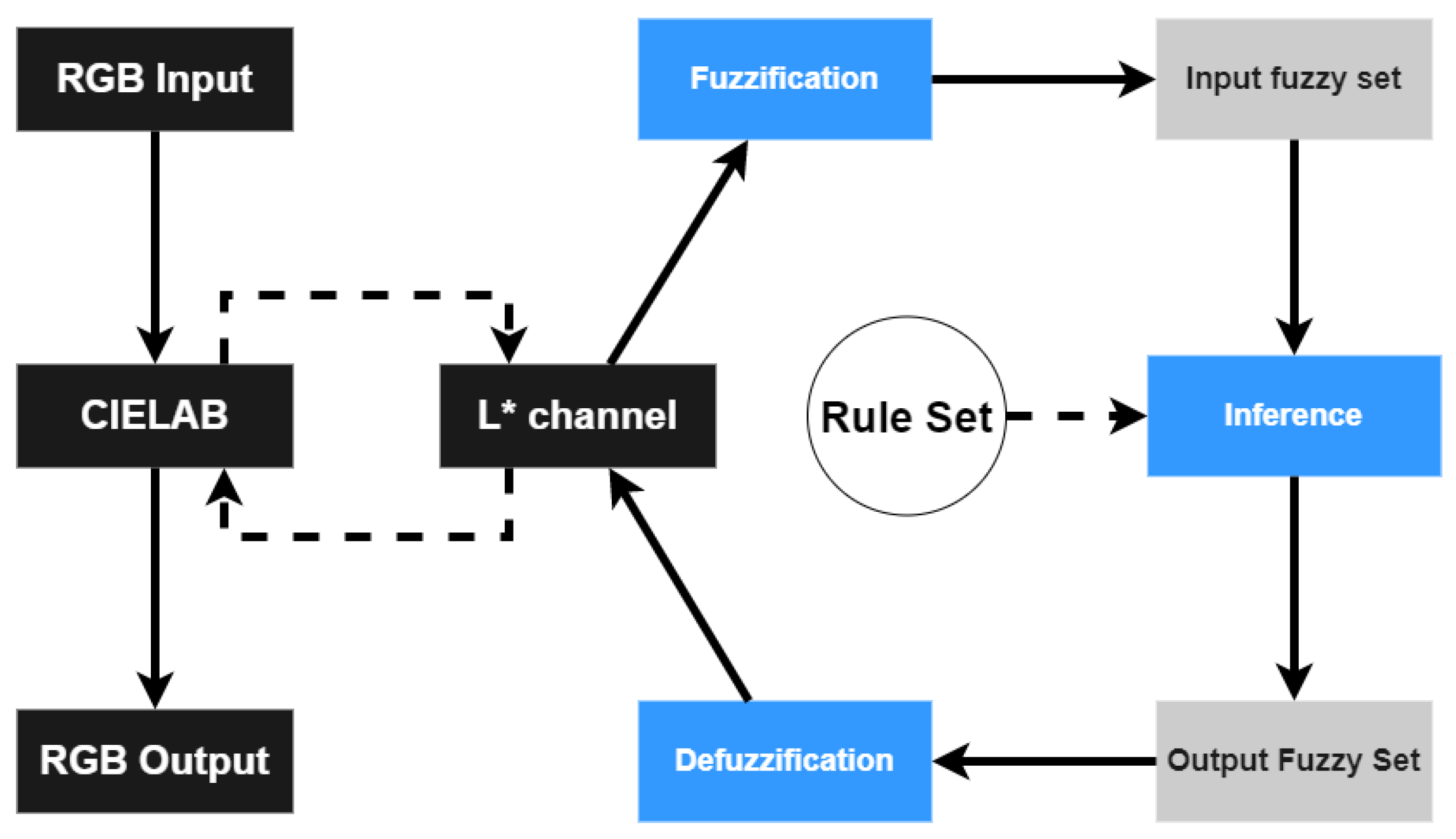
4. Proposed Image Preprocessing with Fuzzy Contrast Enhancement (FCE)

Preprocessing of a dataset when performing artificial intelligence (AI) tasks can ensure data fidelity and continuity. In this section, we implement a preprocessing step to improve the quality and contrast of the created dataset (Section 6.1) before executing the AI algorithms. It is anticipated that the proposed fuzzy contrast enhancement (FCE) preprocessing step will improve the quality of the dataset by increasing the contrast of the images such that machine learning architectures will be able to more easily identify the features differentiating the classes of images in the dataset, leading to higher classification accuracy. To perform FCE, the RGB images were first transformed to the CIELAB color space, and then their intensity component was amplified using fuzzy logic. Conversion to and from the CIELAB color space was accomplished using the OpenCV package available for Python [42]. Amplification of the images’ intensity components was performed through custom software using the Python language and the NumPy package available for Python [43].

4.1. CIELAB Color Space

CIELAB is a three-dimensional device-independent color space model that represents the entire range of human photopic (daylight) vision. It is known to better mimic human vision which helps to identify small differences in color, and alter and isolate specific channels of the image. In an RGB image, the three present channels are red, green, and blue; thus, changing one of these three values will change the overall appearance of the image, but only based on color. In contrast, CIELAB color space has different channels that not only involve the color but also the intensity/lightness of an image.

The CIELAB color space was built from three channels that are perpendicular to one another. The a*, b*, and L* channels are relative to colors green to red, blue to yellow, and black to white, respectively [44]. The L* channel represents pixel intensity and closely matches human perception of lightness or achromatic colors, the shades of grey. For example, L* = 0 and L* = 1 denote pure black and white, respectively. Each color is represented by a color point (L*, a*, b*) in the color space [44]. CIELAB color space is selected because it is useful for detecting and predicting small differences in color of the images.

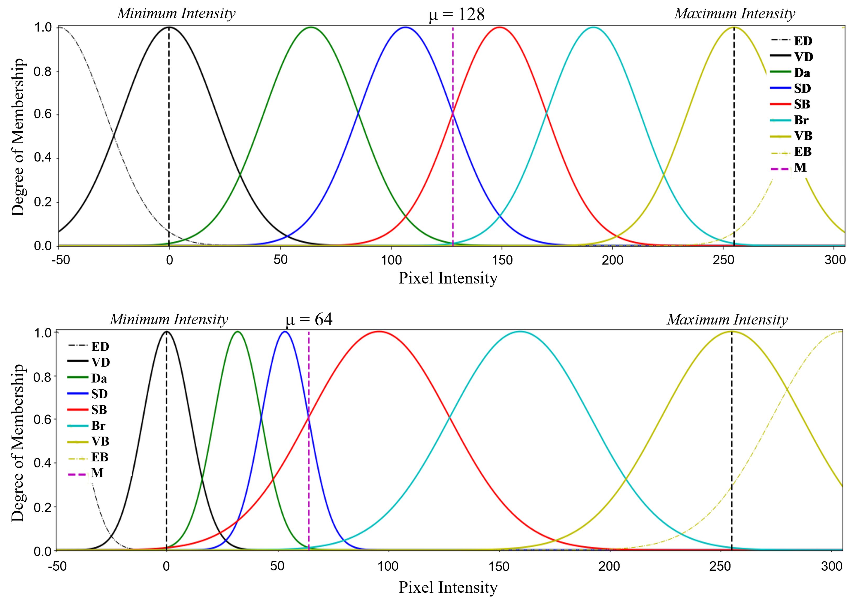
4.2. Fuzzification of Image Pixel Intensity

Fuzzy logic refers to the generalization of a real number, which is a fuzzy number. It introduces a connected set of possible values, where each value has a weight between 0 and 1. Therefore, it is possible to use fuzzy numbers in the area between two values so that a certain classification or result is not rigidly bound to either one of the two values. In this paper, fuzzy logic is selected for contrast enhancement due to its simplicity and robust outcomes, particularly in classification problems, where values exhibit confidence intervals.

To perform FCE, fuzzy logic rules were used to amplify channel L* (pixel intensity) with a value of 0 being black and 255 being pure white. After isolating the L* channel in the CIELAB color space, the image undergoes fuzzification using the specified fuzzy rule set [21,45]. This rule set is comprised of a predefined inventory of interval values in which the L* of each pixel is categorized. Gaussian membership functions were used to establish these intervals using if-then rules. The functions vary according to each set of intervals defined for the L* value of the pixel. In this setting, each of the intervals get a classification title: “Extremely Dark (ED)”, “Very Dark (VD)”, “Dark (Da)”, “Slightly Dark (SD)”, “Slightly Bright (SB)”, “Bright (Br)”, “Very Bright (VB)”, and “Extremely Bright (EB)” (see Figure 4). While the intervals for each of these classifications are different, the base equation is the same, a Gaussian function is given by (1)

$$\mu (x;\mu ,s)=exp(-\frac{1}{2}{(\frac{x-\mu }{s})}^2)$$

(1)

where x is the pixel value, $\mu$ or ‘M’ is the mean (the average pixel value of the given image) and s is the standard deviation of pixel values in the given image. Figure 4 shows the fuzzy membership functions for $\mu =128$.

After assigning the new classification to the pixel, the proposed fuzzy rule set becomes operational (Figure 5). The execution involves utilizing fuzzy rules for elevating all classifications by one level to achieve contrast enhancement (Algorithm 1, [45]). For example, if a pixel receives a classification of “Very Dark (VD)” then according to our fuzzy rule set, the new fuzzified classification would be “Extremely Dark (ED)”, and so on. This rule set eliminates any “Slightly Bright (SB)” or “Slightly Dark (SD)” classifications. By applying Algorithm 1 to images of wind turbines, these contrast modifications will be applied as defined by the if-then rules. This will lead to contrast enhancement in the images, where an increase in the overall accuracy of the ML architectures is anticipated. A visualization of images processed with this FCE algorithm is given in Figure 6, and results indicating the effectiveness of FCE are presented in Section 7 as well as

Table 2. Comparison of VGG19, Xception, and SVM without the proposed FCE using derived performance metrics averaged over ten trials.

Algorithm	Accuracy	Precision	Hit Rate	Miss Rate	Specificity	Fall-Out	F1 Score
Xception	99.00%	99.21%	98.78%	1.21%	99.21%	0.78%	98.99%
VGG19	98.26%	98.34%	98.16%	1.83%	98.36%	1.64%	98.25%
SVM	90.31%	91.00%	87.15%	12.84%	94.01%	5.98%	90.12%

and

Table 3. Comparison of VGG19, Xception, and SVM with the proposed FCE using derived performance metrics averaged over ten trials.

Algorithm	Accuracy	Precision	Hit Rate	Miss Rate	Specificity	Fall-Out	F1 Score
Xception	99.18%	99.50%	98.84%	1.15%	99.51%	0.49%	99.17%
VGG19	97.99%	97.05%	98.87%	1.12%	97.14%	2.85%	97.95%
SVM	95.48%	95.63%	94.75%	5.25%	96.23%	3.76%	95.48%

and Figure 7 and Figure 8.

Algorithm 1 Fuzzy Logic-Based Image Contrast Enhancement

Input: Aerial RGB image Output: Aerial RGB image with fuzzy contrast enhancement   1: Convert input image from RGB to CIELAB color space and calculate the average pixel intensity ($\mu$) of the image   2: Fuzzification: For each pixel, calculate degree of membership of each class based on pixel intensity and $\mu$ value; intensity $\in [0,255]$   3: Inference: Calculate the output fuzzy set from the input pixel intensity based on the following rule set: If input is “Very Dark (VD)” then output is “Extremely Dark (ED)” If input is “Dark (Da)” then output is “Very Dark (VD)” If input is “Slightly Dark (SD)” then output is “Dark (Da)” If input is “Slightly Bright (SB)” then output is “Bright (Br)” If input is “Bright (Br)” then output is “Very Bright (VB)” If input is “Very Bright (VB)” then output is “Extremely Bright (EB)”.   4: Defuzzification: For each pixel, calculate the centroid value of its output fuzzy set; centroid $\in [-50,305]$   5: Normalize output pixel intensity from $[-50,305]$ to $[0,255]$   6: Merge modified L* channel to the original a*b* channels   7: Convert output image from CIELAB color space to RGB

5. Hyperparameter Tuning

The three ML approaches used in this research (VGG19, Xception, and SVM) were further tweaked to tune the network architectures for the detection of wind turbines through the selection of hyperparameters: parameters of a network that can be modified before training to improve model performance [46]. As the number of hyperparameters can increase significantly, the process of determining the ideal hyperparameters for the network becomes computationally expensive and time-consuming. Therefore, a method of determining productive hyperparameters must be used [46]. Due to its association with the popular deep learning framework Keras and its strong results, KerasTuner was used to tune the hyperparameter values [23,47]. Of the hyperparameter algorithms provided by KerasTuner, Bayesian optimization and the Hyperband algorithm were explored. Bayesian optimization is a very efficient method as it takes into account past hyperparameter performance for the future decision. Hyperband is beneficial because it early-stops poor-performing sets of hyperparameter optimization in exchange for more emphasis on more promising sets of hyperparameters. Additionally, RandomSearch was tested briefly until it was apparent the other options were superior. RandomSearch is a method in which random combinations of hyperparameters are selected and used to train a model, resulting in reducing the number of hyperparameter configurations searched [47]. The Bayesian optimization hyperparameter algorithm assumes the optimization function comes from a Gaussian process. Based on all previous evaluations, the algorithm builds a probabilistic function on this assumption and attempts to optimize hyperparameters. Bayesian optimization is a black box approach, as the function being optimized is never directly identified [48].

The Hyperband algorithm employs a different approach called successive halving where each hyperparameter configuration is given a computational budget. After the budget is consumed, the algorithm filters through and determines the worst-performing configurations, terminating them. The remaining configurations are given another computational budget and the process continues until the most performant configuration remains. The algorithm assumes that all configurations can be stopped early and evaluated [49].

5.1. Hyperparameter Categories

Many categories of hyperparameters are available: some are specific to the type of model being used and the task being performed; others have a broader scope and can be applied to multiple models. The tuning performed in this research focuses on the latter. Specifically, the hyperparameters explored in this research include the network’s optimizer type, activation function, batch size, loss function, and dropout, which are explored in the remainder of this section. Each hyperparameter and its corresponding values were selected and optimized using a reasonably wide search space paired with a series of case studies. Hyperparameters and values that performed well were used in future case studies while those that performed suboptimally were dropped from future consideration. The values of numerical hyperparameters, such as batch size and dropout, were selected from a pool of practical size; the values of other hyperparameters, such as optimizer and activation function, were selected using the pool of values available through the Keras software. The impact of hyperparameter selection and values on the performance of each machine learning architecture is presented in the case studies of Section 6.

5.1.1. Optimizer

A key hyperparameter experimented with was the optimizer. An optimizer is an equation or a set of equations that update the values of the model weights during backpropagation by traversing the gradients of the loss function, which can be represented as a multidimensional curve. The purpose of an optimizer is to find a local minimum on this curve to increase model accuracy. Various optimizers exist, and each implements a different gradient-traversal method. The optimizers explored here include Adam, NAdam, AdaMax, and RMSProp [23,50,51,52].

5.1.2. Activation Functions

Activation functions are nonlinear layers in neural networks that require inputs to be greater than a critical value to be passed to further layers. They prevent the network from collapsing into a singular matrix and enable the network to perform more complex tasks. Selection of the proper activation function can make a significant difference to the performance of the network [23,53,54,55,56,57,58].

5.1.3. Batch Size

In calculations for gradient descent, two schools of thought are presented for the management of training sources: stochastic gradient descent and batch gradient descent. The former suggests updating the model with each training data point; the latter suggests updating the model after processing each training data point reference. However, both stochastic gradient descent and batch gradient descent have drawbacks that can be analyzed to determine which will be more effective depending on the task.

A trade-off exists between the two methods. Large batch sizes benefit heavily from the highly parallel nature of machine learning; therefore, the training execution time can be greatly reduced. However, larger batch sizes require large pools of available memory to perform calculations and can be trapped in local minima in the loss function. Smaller batch sizes tend to be more noisy, allowing optimizers to break out of local minima and saddle points [59].

5.1.4. Loss Function

The loss function defines the margin of error of image classification in the network during training. Three loss functions were explored here: categorical cross-entropy, binary cross-entropy, and Kullback–Leiber (KL) divergence [60,61].

5.1.5. Dropout

Dropout is a method to prevent overfitting. Using the dropout during training, a percentage of nodes from fully connected layers are dropped from the network, preventing their weights from being used or updated. This forces the network to prioritize more than one major network path and avoid overfitting. It also simulates training multiple subnetworks and combining the results into the overall network [62].

6. Experimental Results

6.1. Dataset Overview and Characteristics

The machine learning algorithms introduced in Section 2 and Section 3 were trained on the created dataset of 4500 RGB images. The dataset contains two classes of images: those with wind turbines (WT class) and those without (NWT class). The WT class has 2250 images that contain a small-scale wind turbine (12V Primus Air Max wind turbine) assembled at Utah Valley University (UVU). This wind turbine is shown in Figure 6. These images were captured on a Zenmuse L1 RGB camera that was mounted on a DJI Matrice 300 RTK drone. To ensure diversity and relevance to real-world wind turbine detection scenarios, emphasis was placed on creating dataset images with diverse angles and distances to the wind turbine to simulate perspectives that are commonly observed from a drone-mounted camera in a wind turbine farm. Additionally, images were captured in multiple weather conditions at various times of day to ensure the dataset was robust. The NWT class also has 2250 images that were taken in the same location as the WT images, so both sets have similar backgrounds including trees and sky. The NWT class also contains images captured at multiple times of day with various weather patterns. Additionally, all images in the dataset were manually validated to ensure that each image had been placed in the correct class and that each image was an accurate representation of the class it had been placed in.

The analysis of machine learning algorithms in this paper prioritized fast training times so that more experimentation and iterative improvement could occur. As a result, the images in the dataset were downscaled to $210\times 210$ pixels. Additionally, the dataset is separated into 3150 training images and 1350 test images to verify the performance of the machine learning algorithms using previously unseen data. A selection of images from this dataset is displayed in Figure 6, where Figure 6a,b show sample images from the NWT and WT classes, respectively. Figure 6c,d show corresponding images after the application of the proposed FCE preprocessing technique of Section 4.

6.2. VGG19 Experimental Results

The VGG19 network used the weights of the ImageNet dataset to expedite feature extraction, and the dense classifier on top helped in identifying whether there was a turbine in the image or not. The dense classifier had a total of six layers. The VGG base and dense classifier were trained concurrently for better results as described in Section 2.1. The number of neurons in the last layers depends on the number of classes in the training data, which is an important detail to remember. Since there are only two classes (turbine or no turbine) in the training database, the final layer contains two neurons. The VGG19 network underwent several hyperparameter searches and tuning in order to determine the combination of parameters that would perform the best on the dataset. This took place in Case Studies A1–A3 on images downscaled to $135\times 85$ pixels so that successful hyperparameters could be identified more quickly due to the increased training speeds associated with smaller images. Case Studies A4–A5 apply the resulting hyperparameters to the $210\times 210$ pixel dataset described at the start of this section for evaluation of fuzzy contrast enhancement. The sections that follow outline the design and results of these studies.

6.2.1. VGG19 Case Study A1

Case Study A1 used the RMSProp optimizer in grid search for the VGG19 network. The network’s dropout rate, image batch size, and optimizer learning rate were the hyperparameters selected for the grid search, while the validation accuracy was used to measure optimization. The image batch size was tested with values of 2, 5, 10, 15, 30, 50, and 120, the optimizer learning rate with values of ${10}^{-5}$, ${10}^{-4}$, $5\times {10}^{-4}$, ${10}^{-3}$, ${10}^{-2}$, and ${10}^{-1}$, and the dropout rate with values of 10%, 20%, and 30%. Each set of hyperparameters was trained on the wind turbine dataset for 100 iterations.

Table 4. Top three hyperparameters for VGG19 Case Studies A1–A3 with batch size (BS), learning rate (LR), dropout rate (DR), and validation accuracy (VA).

Case Study	No.	BS	LR	DR	Validation Accuracy (VA)
Case Study A1	1	30	0.0005	30%	98.36%
	2	60	0.0001	30%	98.35%
	3	30	0.001	20%	98.32%
Case Study A2	1	20	0.0005	20%	98.35%
	2	60	0.0005	30%	98.30%
	3	60	0.0001	20%	98.29%
Case Study A3	1	300	0.0001	30%	98.41%
	2	60	0.0001	20%	98.39%
	3	150	0.0001	20%	98.25%

lists the best-performing hyperparameters for each search.

6.2.2. VGG19 Case Study A2

Since the VGG19 network received beneficial results with RMSProp, Case Study A2 used the same combination but with a different search space of the hyperparameters and a different search algorithm. The network’s dropout rate, image batch size, and optimizer learning rate were again chosen as the hyperparameters, but this time for the Bayesian optimization search. The validation accuracy was used as a measure to be optimized. The image batch size was tested with values of 20, 50, 100, 150, 300, 350, and 400, and the dropout rate was tested with values of 20%, 30%, and 50%. The optimizer learning rate was tested with the same values as Case Study A1. The wind turbine dataset was used to train for 100 iterations of all hyperparameter options. Table 4 lists the best-performing hyperparameters for each search. The performance of the VGG19 architecture with RMSProp in Case Study A2 was comparable to results from Case Study A1.

6.2.3. VGG19 Case Study A3

This case study is very similar to Case Study A2. Since VGG19 performed well with RMSProp, the same hyperparameters were used in Case Study A3. The same search space for the hyperparameters was also used, but it was implemented via the Hyperband algorithm instead of Bayesian or grid search. The best-performing hyperparameters for each search are listed in Table 4. Across Case Studies A1 through A3, all combinations of hyperparameter values performed reasonably well.

6.2.4. VGG19 Case Study A4

To obtain the final evaluation of VGG19’s performance for comparison with the other deep learning methods explored, VGG19 was retrained using only the top performing set of hyperparameters from Table 4; each image from the created dataset was then classified by this trained network. The results were gathered into a confusion matrix from which performance metrics such as accuracy and precision were calculated. The results of this process were averaged across 10 separate runs and the highest accuracy overall was recorded. The resulting averaged performance metrics, as well as the confusion matrix with the highest accuracy for this model, are given in Figure 7a.

6.2.5. VGG19 Case Study A5

This case study tested the impact of fuzzy contrast enhancement as a preprocessing step on the image dataset for the VGG19 network. Its procedure replicated that of Case Study A4 in many ways. However, it differed in the addition of image preprocessing and a lower batch size of 128 rather than 300 which was used previously. These results are shown in Figure 8a and Table 3.

6.3. Xception Experimental Results

Six case studies of hyperparameter searches were conducted on the Xception network to find the combination which performed best on the wind turbine dataset. In order to increase the speed of hyperparameter selection, Case Studies B1–B4 used images downscaled to $135\times 85$ pixels. Once hyperparameters had been identified which consistently performed well, they were applied to the larger $210\times 210$ pixel images for evaluation of fuzzy contrast enhancement in Case Studies B5–B6. More information on the performance of each is described in the sections that follow.

6.3.1. Xception Case Study B1

This case study paired the Xception network with the Adam optimizer while image batch size, optimizer learning rate, and the network’s dropout rate were allowed to vary as hyperparameters. The image batch size was tested with values of 1, 5, 10, 20, 32, 64, and 128, the optimizer learning rate was tested with values of ${10}^{-5}$, ${10}^{-4}$, $5\times {10}^{-4}$, ${10}^{-3}$, $2\times {10}^{-2}$, and ${10}^{-2}$, and the network dropout rate was tested with values ranging from 0% to 95% in 5% increments. For this case study, the hyperparameters were tuned with KerasTuner’s RandomSearch algorithm. Additionally, the results were averaged from three independent executions, and each search was trained for 30 epochs but set to stop early if epoch loss did not improve for three epochs.

The results from this case study are visualized in Figure 9. Notably, the batch sizes in the middle of the selected range (5, 10, 20, and 32) consistently performed with high accuracies (90–95%), while the extremes in the tested batch size range (1, 64, and 128) consistently had low accuracies (50–60%). The best hyperparameters are given in

Table 5. Top three hyperparameters for Xception Case Studies B1-B4 with batch size (BS), loss (L), optimizer (O), dropout layer (DL), dropout rate (DR), optimizer learning rate (LR), Adam Beta1 (B1), Adam Beta2 (B2), Adam Epsilon (E), and Adam AMSGrad (AMSG). In all of these case studies, we used the ReLU activation function and Sigmoid was utilized as the final layer activation function.

Case Study	No.	BS	L	O	DL	DR	LR	B1	B2	E	AMSG	Accuracy
Case B1	1	20	BC	Adam	True	60%	$5\times {10}^{-4}$	0.9	0.999	${10}^{-7}$	False	95.321%
	2	5	BC	Adam	True	10%	${10}^{-4}$	0.9	0.999	${10}^{-7}$	False	94.509%
	3	5	BC	Adam	True	80%	${10}^{-4}$	0.9	0.999	${10}^{-7}$	False	94.209%
Case B2	1	32	BC	Adam	False	-	${10}^{-5}$	0.9	0.999	${10}^{-7}$	False	88.953%
	2	32	BC	Adam	False	-	${10}^{-5}$	0.9	0.999	${10}^{-7}$	False	88.590%
	3	32	BC	Adam	False	-	${10}^{-5}$	0.9	0.999	${10}^{-7}$	False	88.462%
Case B3	1	10	BC	Adam	True	45%	$5\times {10}^{-4}$	0.9	0.99	${10}^{-7}$	True	93.686%
	2	20	BC	Adam	True	35%	${10}^{-3}$	0.0	0.99	${10}^{-7}$	True	93.103%
	3	5	BC	Adam	True	25%	$5\times {10}^{-4}$	0.0	0.0	${10}^{-7}$	True	89.103%
Case B4	1	5	BC	Adam	True	45%	$2\times {10}^{-3}$	0.0	0.0	${10}^{-1}$	True	96.058%
	2	10	BC	Adam	True	20%	${10}^{-4}$	0.0	0.999	${10}^{-7}$	False	94.872%
	3	5	BC	Adam	True	20%	${10}^{-4}$	0.9	0.9999	${10}^{-7}$	True	94.359%

under Case Study B1.

6.3.2. Xception Case Study B2

In this case study, the hyperparameters were tuned using KerasTuner’s Bayesian optimization tuner. These hyperparameters included the dropout ratio, the learning rate, the activation function used in Xception’s final layer, the optimizer paired with the Xception network, and conditional inclusion of the dropout layer. The optimizer was tested with Adam and NAdam, the final layer activation function was tested with Softmax and Sigmoid, and the dropout ratio was tested with values of 0% through 90% in 10% increments when the dropout layer was included.

During training, the learning rate was allowed to vary logarithmically with a minimum value of ${10}^{-5}$ and a maximum value of ${10}^{-1}$. This assigns equal probabilities to each order of magnitude range [47]. The results from Case Study B2 are given in Figure 10, where it can be seen that Softmax consistently performed poorly as Xception’s final layer activation function, while Sigmoid consistently performed well. Softmax was removed from further trials for this reason. The hyperparameters that consistently performed well in this case study are listed in Table 5 under Case Study B2.

6.3.3. Xception Case Study B3

This case study focused on tuning the Adam optimizer’s learning rate, Beta1, Beta2, Epsilon, and AMSGrad inputs as well as dropout ratio and batch size using Bayesian optimization. Each combination of hyperparameters was independently executed ten times, and the results of each were averaged to obtain each search’s final outcomes.

The hyperparameters were tested with values of ${10}^{-4}$, $5\times {10}^{-4}$, ${10}^{-3}$, and $2\times {10}^{-3}$ for the learning rate, 0.0 and 0.9 for Beta1, 0.0, 0.99, 0.999, and 0.9999 for Beta2, ${10}^{-7}$, ${10}^{-1}$, and $1.0$ for Epsilon, true or false for AMSGrad, and 0% through 50% in 5% increments for the dropout ratio. The batch sizes were tested with the same values as Case Study B1. The available values for Beta1 and Beta2 were selected based on [63], with Beta2 being modified to include a value of 0.0. The available values for Epsilon were selected from the Keras documentation. The results from Case Study B3 are visualized in Figure 11, and the hyperparameters with the highest average accuracies from this case study are listed in Table 5 under Case Study B3. The hyperparameters with the consistent best performance had batch sizes in the middle of the tested range (5, 10, 20) and dropout ratios in the upper half of the tested range (25–45%).

6.3.4. Xception Case Study B4

This trial used the same hyperparameters with the same tested values as Case Study B3, but they were tuned with the Hyperband algorithm rather than the Bayesian optimization algorithm. The results are visualized in Figure 12, and the hyperparameters that had the highest averaged accuracies are given in Table 5 under Case Study B4. In Figure 12, note that the accuracies at the low-end of the scale are about 88%. In other case studies, the low end of the scale for accuracies ranged from 50% to about 68%. The Hyperband algorithm resulted in higher accuracies.

Across Case Studies B1 through B4, very low and very high batch sizes (below 5 and above 64) tended to perform poorly. Additionally, the NAdam optimizer and the Softmax final layer activation function performed poorly in combination with the other hyperparameters and values selected in Case Studies B1 through B4. The inclusion of the dropout layer was also a key hyperparameter: performance significantly decreased when the dropout layer was not included in the architecture. Overall, the best results were attained when using medium-range batches sizes (5 through 32), the Adam optimizer, the Sigmoid final layer activation function, and when a dropout layer was included in the architecture.

6.3.5. Xception Case Study B5

In this case study, fine-tuning was implemented for the Xception network structure. The model was initialized with weights pretrained on the ImageNet dataset and given a densely connected final layer. Where appropriate, the model was assigned with the top set of hyperparameters from Table 5. To prepare the network for fine-tuning, the pretrained weights were frozen, while the final dense layer was trained on the wind turbine dataset. During fine-tuning, the final seventeen layers, including the densely connected layer, were unfrozen and trained with one-tenth of the learning rate used in the fine-tuning preparation stage. The model was evaluated using the process described in VGG19 Case Study A4. The results are illustrated in Figure 7b and Table 2.

6.3.6. Xception Case Study B6

This case study analyzed the effect of implementing fuzzy contrast enhancement as a preprocessing step for the Xception network. Its procedure mirrored that of Case Study B5 with the only difference being the addition of image preprocessing. These results are given in Figure 8b and Table 3.

6.4. SVM Experimental Results

Experiments in this section were undertaken to explore the effects of the proposed FCE image preprocessing of Section 4 on the performance and accuracy of the SVM algorithm. Four SVM case studies were conducted, encompassing default hyperparameter settings and Bayesian optimization, both with and without FCE image preprocessing.

6.4.1. SVM Case Study C1

In the first case study with SVM, the default hyperparameters were used. The model was built using the Scikit-learn library in Python and no hyperparameter values were altered. The default hyperparameter values are C = 1, Gamma = Scale, and Kernel = rbf. These hyperparameter values are the same for any SVM built using Scikit-learn in Python.

6.4.2. SVM Case Study C2

The second case study with SVM is executed using Bayesian optimization instead of the default hyperparameters setting. This study aims to identify the optimal combination of hyperparameters to attain the highest accuracy for our model. The results are presented in Figure 7c and Table 2.

6.4.3. SVM Case Study C3

The third SVM case study mirrors Case Study C1 by relying on default hyperparameters. However, it incorporates the proposed FCE procedure outlined in Section 4. Consequently, a preprocessing step is integrated into the SVM algorithm to modulate the intensity of all images within the generated dataset. This study aims to establish a baseline accuracy when implementing fuzzy contrast enhancement, providing a benchmark for comparison with the accuracy achieved in the subsequent section.

6.4.4. SVM Case Study C4

The ultimate SVM study integrated elements from both Case Study C2 and C3, incorporating both Bayesian optimization and the proposed FCE preprocessing step of Section 4. The application of these combined techniques generated the highest accuracy attained by the SVM model. Comprehensive results and details of this conclusive case study are presented in Figure 8c and Table 3.

7. Conclusions

This paper examines and contrasts the impact of applying fuzzy contrast enhancement (FCE) as an image preprocessing algorithm to various strategies for detecting the presence of wind turbines in RGB images, an initial key aspect of autonomous wind turbine inspection. The three methods under investigation are VGG19, Xception, and SVM. The primary contributions of this paper encompass the following:

• A comprehensive exploration, implementation, and comparison of three distinct machine learning algorithms, comprising two convolutional neural networks and the SVM algorithm. These algorithms are utilized to classify whether RGB images contain wind turbines.
• The application of the proposed fuzzy contrast enhancement (FCE) data preprocessing step to the VGG19, Xception, and SVM machine learning algorithms, accompanied by a comparison of their conventional performance against their performance when augmented by this preprocessing step.
• The creation of a novel Primus Air Max wind turbine classification dataset, consisting of 4500 RGB images, and its utilization to assess the performance of the implemented VGG19, Xception, and SVM algorithms.

Based on our analysis, primary conclusions are as follows:

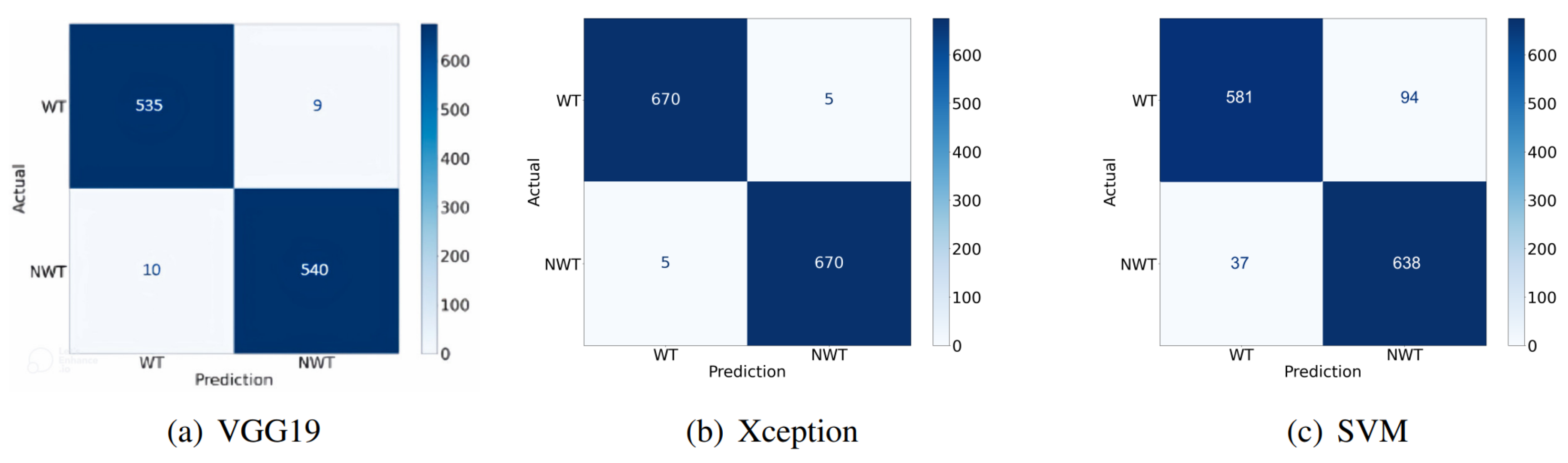
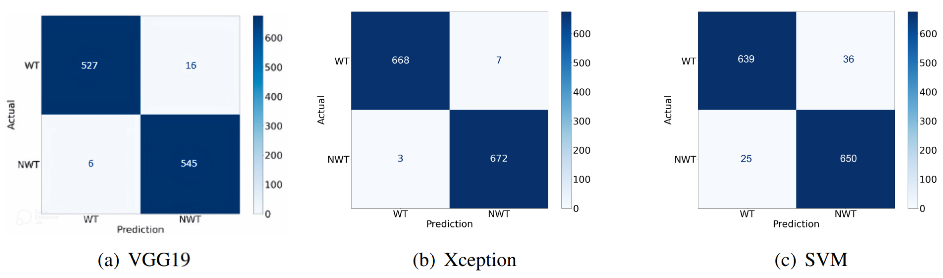
• The assessed convolutional neural networks, namely Xception and VGG19, demonstrated commendable performances with accuracies above 98%. In contrast, as anticipated, the SVM algorithm exhibited a less favorable accuracy of around 90%.
• The implementation of the proposed FCE results in enhanced accuracy for Xception and SVM, while VGG19 does not experience similar improvements.
• The results presented in Figure 7 and Figure 8 and Table 2 and Table 3 demonstrate that implementing the proposed FCE leads to improvements in accuracy, precision, and F1 score. Specifically, for the Xception model, these metrics increase from 99%, 99.2%, and 98.99% to 99.18%, 99.5%, and 99.18%, respectively. Similarly, for the SVM algorithm, the application of FCE raises accuracy, precision, and F1 score from 90.3%, 91%, and 90.12% to 95.48%, 95.63%, and 95.48%, respectively.

In summary, FCE as a data preprocessing algorithm for wind turbine detection is promising: two of the explored machine learning architectures experienced a performance increase when this algorithm was applied. Future research into autonomous condition monitoring of wind turbines may similarly benefit from applying FCE as a dataset preprocessing step. For future investigations, the authors intend to expand the existing dataset to incorporate RGB images depicting both intact and defective wind turbine blades, with and without cracks. Further enhancements and training of the Xception, VGG19, and SVM algorithms are envisaged to facilitate their utilization in automated drone path planning, enabling the autonomous detection of faults in wind turbine blades.

References

- Lee, J.; Zhao, F. GWEC | Global Wind Report 2022. 2022. Available online: https://gwec.net/wp-content/uploads/2022/03/GWEC-GLOBAL-WIND-REPORT-2022.pdf/ (accessed on 4 September 2022).
- Wang, L.; Zhang, Z.; Long, H.; Xu, J.; Liu, R. Wind Turbine Gearbox Failure Identification With Deep Neural Networks. IEEE Trans. Ind. Inform. 2017, 13, 1360–1368. [Google Scholar] [CrossRef]
- Long, H.; Wang, L.; Zhang, Z.; Song, Z.; Xu, J. Data-Driven Wind Turbine Power Generation Performance Monitoring. IEEE Trans. Ind. Electron. 2015, 62, 6627–6635. [Google Scholar] [CrossRef]
- Ribrant, J.; Bertling, L.M. Survey of Failures in Wind Power Systems With Focus on Swedish Wind Power Plants During 1997–2005. IEEE Trans. Energy Convers. 2007, 22, 167–173. [Google Scholar] [CrossRef]
- Honjo, N. Detail survey of wind turbine generator and electric facility damages by winter lightning. In Proceedings of the 31st Wind Energy Utilization Symposium, 2013; Volume 35, pp. 296–299. Available online: https://www.jstage.jst.go.jp/article/jweasympo/35/0/35_296/_article/-char/en (accessed on 5 December 2023).
- Hahn, B.; Durstewitz, M.; Rohrig, K. Reliability of wind turbines. In Wind Energy; Springer: Berlin/Heidelberg, Germany, 2007; pp. 329–332. [Google Scholar]
- Qiao, W.; Lu, D. A Survey on Wind Turbine Condition Monitoring and Fault Diagnosis—Part I: Components and Subsystems. IEEE Trans. Ind. Electron. 2015, 62, 6536–6545. [Google Scholar] [CrossRef]
- GEV Wind Power. 2021 Wind Turbine Blade Inspection. Available online: https://www.gevwindpower.com/blade-inspection/ (accessed on 4 September 2022).
- Industrial Rope Access Trade Association. IRATA International. Available online: https://irata.org/ (accessed on 26 December 2023).
- Society of Professional Rope Access Technicians. SPRAT. Available online: https://sprat.org/ (accessed on 26 December 2023).
- Coffey, B. Taking Off: Nevada Drone Testing Brings Commercial UAVs Closer to Reality. 2019. Available online: https://www.ge.com/news/reports/taking-off-nevada-drone-testing-brings-commercial-uavs-closer-to-reality (accessed on 4 September 2022).
- Clobotics. Wind Services. Available online: https://clobotics.com/wind/ (accessed on 26 December 2023).
- Arthwind. Arthwind—Visibility and Prediction. Available online: https://arthwind.com.br/en/ (accessed on 26 December 2023).
- N’Diaye, L.M.; Phillips, A.; Masoum, M.A.S.; Shekaramiz, M. Residual and Wavelet based Neural Network for the Fault Detection of Wind Turbine Blades. In Proceedings of the 2022 Intermountain Engineering, Technology and Computing (IETC), Orem, UT, USA, 13–14 May 2022; pp. 1–5. [Google Scholar] [CrossRef]
- Seibi, C.; Ward, Z.; Masoum, M.A.S.; Shekaramiz, M. Locating and Extracting Wind Turbine Blade Cracks Using Haar-like Features and Clustering. In Proceedings of the 2022 Intermountain Engineering, Technology and Computing (IETC), Orem, UT, USA, 13–14 May 2022; pp. 1–5. [Google Scholar] [CrossRef]
- Seegmiller, C.; Chamberlain, B.; Miller, J.; Masoum, M.A.S.; Shekaramiz, M. Wind Turbine Fault Classification Using Support Vector Machines with Fuzzy Logic. In Proceedings of the 2022 Intermountain Engineering, Technology and Computing (IETC), Orem, UT, USA, 13–14 May 2022; pp. 1–5. [Google Scholar] [CrossRef]
- Pinney, B.; Duncan, S.; Shekaramiz, M.; Masoum, M.A.S. Drone Path Planning and Object Detection via QR Codes; A Surrogate Case Study for Wind Turbine Inspection. In Proceedings of the 2022 Intermountain Engineering, Technology and Computing (IETC), Orem, UT, USA, 13–14 May 2022; pp. 1–6. [Google Scholar] [CrossRef]
- IBM. What Is Machine Learning? Available online: https://www.ibm.com/cloud/learn/machine-learning (accessed on 17 September 2022).
- IBM. What Are Convolutional Neural Networks. Available online: https://www.ibm.com/cloud/learn/convolutional-neural-networks (accessed on 8 September 2022).
- O’Shea, K.; Nash, R. An Introduction to Convolutional Neural Networks. arXiv 2015, arXiv:1511.08458. [Google Scholar] [CrossRef]
- Rahman, R.; Tanvir, S.; Anwar, M.T. Unique Approach to Detect Bowling Grips Using Fuzzy Logic Contrast Enhancement. In Proceedings of the 2021 IEEE International Conference on Artificial Intelligence in Engineering and Technology (IICAIET), Kota Kinabalu, Malaysia, 13–15 September 2021; pp. 1–6. [Google Scholar] [CrossRef]
- Chutani, G.; Bohra, H.; Diwan, D.; Garg, N. Improved Alzheimer Detection using Image Enhancement Techniques and Transfer Learning. In Proceedings of the 2022 3rd International Conference for Emerging Technology (INCET), Belgaum, India, 27–29 May 2022; pp. 1–6. [Google Scholar] [CrossRef]
- Keras. 2015. Available online: https://keras.io (accessed on 24 June 2022).
- Simonyan, K.; Zisserman, A. Very Deep Convolutional Networks for Large-scale Image Recognition. arXiv 2014, arXiv:1409.1556. [Google Scholar]
- Sarkar, D. A comprehensive hands-on guide to transfer learning with real-world applications in deep learning. Towards Data Sci. 2018, 20, 4. [Google Scholar]
- Yalcin, O.G. 4 Pre-Trained CNN Models to Use for Computer Vision with Transfer Learning. Towards Data Sci. 2020. Available online: https://towardsdatascience.com/4-pre-trained-cnn-models-to-use-for-computer-vision-with-transfer-learning-885cb1b2dfc (accessed on 5 December 2023).
- Chollet, F. Deep Learning with Python; Simon and Schuster: New York, NY, USA, 2021. [Google Scholar]
- Szegedy, C.; Liu, W.; Jia, Y.; Sermanet, P.; Reed, S.; Anguelov, D.; Erhan, D.; Vanhoucke, V.; Rabinovich, A. Going deeper with convolutions. In Proceedings of the 2015 IEEE Conference on Computer Vision and Pattern Recognition (CVPR), Boston, MA, USA, 7–12 June 2015; pp. 1–9. [Google Scholar] [CrossRef]
- Ioffe, S.; Szegedy, C. Batch normalization: Accelerating deep network training by reducing internal covariate shift. In Proceedings of the International Conference on Machine Learning, Lille, France, 6–11 July 2015; pp. 448–456. [Google Scholar]
- Szegedy, C.; Vanhoucke, V.; Ioffe, S.; Shlens, J.; Wojna, Z. Rethinking the Inception Architecture for Computer Vision. In Proceedings of the 2016 IEEE Conference on Computer Vision and Pattern Recognition (CVPR), Las Vegas, NV, USA, 27–30 June 2016; pp. 2818–2826. [Google Scholar] [CrossRef]
- Chollet, F. Xception: Deep Learning with Depthwise Separable Convolutions. In Proceedings of the 2017 IEEE Conference on Computer Vision and Pattern Recognition (CVPR), Honolulu, HI, USA, 21–26 July 2017; pp. 1800–1807. [Google Scholar] [CrossRef]
- Rahman, M.R.; Tabassum, S.; Haque, E.; Nishat, M.M.; Faisal, F.; Hossain, E. CNN-based Deep Learning Approach for Micro-crack Detection of Solar Panels. In Proceedings of the 2021 3rd International Conference on Sustainable Technologies for Industry 4.0 (STI), Dhaka, Bangladesh, 18–19 December 2021; pp. 1–6. [Google Scholar] [CrossRef]
- Roopashree, S.; Anitha, J. DeepHerb: A Vision Based System for Medicinal Plants Using Xception Features. IEEE Access 2021, 9, 135927–135941. [Google Scholar] [CrossRef]
- Chen, B.; Liu, X.; Zheng, Y.; Zhao, G.; Shi, Y.Q. A Robust GAN-Generated Face Detection Method Based on Dual-Color Spaces and an Improved Xception. IEEE Trans. Circuits Syst. Video Technol. 2022, 32, 3527–3538. [Google Scholar] [CrossRef]
- Hui, J.; Du, M.; Ye, X.; Qin, Q.; Sui, J. Effective Building Extraction From High-Resolution Remote Sensing Images With Multitask Driven Deep Neural Network. IEEE Geosci. Remote Sens. Lett. 2019, 16, 786–790. [Google Scholar] [CrossRef]
- Pupale, R. Support Vector Machines (SVM)—An Overview. 2018. Available online: https://towardsdatascience.com/https-medium-com-pupalerushikesh-svm-f4b42800e989 (accessed on 24 June 2022).
- Kobaiz, A.R.; Ghrare, S.E. Behavior of LSSVM and SVM channel equalizers in non-Gaussian noise. In Proceedings of the 2014 International Conference on Computer, Communications, and Control Technology (I4CT), Langkawi, Malaysia, 2–4 September 2014; pp. 407–410. [Google Scholar] [CrossRef]
- Saha, N.; Show, A.K.; Das, P.; Nanda, S. Performance Comparison of Different Kernel Tricks Based on SVM Approach for Parkinson’s Disease Detection. In Proceedings of the 2021 2nd International Conference for Emerging Technology (INCET), Belagavi, India, 21–23 May 2021; pp. 1–4. [Google Scholar] [CrossRef]
- Jiu, M.; Pustelnik, N.; Chebre, M.; Janaqv, S.; Ricoux, P. Multiclass SVM with graph path coding regularization for face classification. In Proceedings of the 2016 IEEE 26th International Workshop on Machine Learning for Signal Processing (MLSP), Vietri sul Mare, Italy, 13–16 September 2016; pp. 1–6. [Google Scholar] [CrossRef]
- Murata, M.; Mitsumori, T.; Doi, K. Overfitting in protein name recognition on biomedical literature and method of preventing it through use of transductive SVM. In Proceedings of the Fourth International Conference on Information Technology (ITNG’07), Las Vegas, NV, USA, 2–4 April 2007; pp. 583–588. [Google Scholar] [CrossRef]
- Pedregosa, F.; Varoquaux, G.; Gramfort, A.; Michel, V.; Thirion, B.; Grisel, O.; Blondel, M.; Prettenhofer, P.; Weiss, R.; Dubourg, V.; et al. Scikit-learn: Machine Learning in Python. J. Mach. Learn. Res. 2011, 12, 2825–2830. [Google Scholar]
- Bradski, G. The OpenCV Library. Dr. Dobb’s J. Softw. Tools 2000, 25, 120–123. [Google Scholar]
- Harris, C.R.; Millman, K.J.; van der Walt, S.J.; Gommers, R.; Virtanen, P.; Cournapeau, D.; Wieser, E.; Taylor, J.; Berg, S.; Smith, N.J.; et al. Array programming with NumPy. Nature 2020, 585, 357–362. [Google Scholar] [CrossRef] [PubMed]
- Zeljkovic, V.; Druzgalski, C.; Mayorga, P. Quantification of acne status using CIELAB color space. In Proceedings of the 2023 Global Medical Engineering Physics Exchanges/Pacific Health Care Engineering (GMEPE/PAHCE), Songdo, Republic of Korea, 27–31 March 2023; pp. 1–6. [Google Scholar]
- Vuong-Le, M.N. Fuzzy Logic—Image Contrast Enhancement. 2020. Available online: https://www.kaggle.com/code/nguyenvlm/fuzzy-logic-image-contrast-enhancement/notebook (accessed on 24 June 2022).
- Talashilkar, R.; Tewari, K. Analyzing the Effects of Hyperparameters on Convolutional Neural Network & Finding the Optimal Solution with a Limited Dataset. In Proceedings of the 2021 International Conference on Advances in Computing, Communication, and Control (ICAC3), Mumbai, India, 3–4 December 2021; pp. 1–5. [Google Scholar] [CrossRef]
- O’Malley, T.; Bursztein, E.; Long, J.; Chollet, F.; Jin, H.; Invernizzi, L.; Bursztein, L. KerasTuner. 2019. Available online: https://github.com/keras-team/keras-tuner (accessed on 1 July 2022).
- Snoek, J.; Larochelle, H.; Adams, R.P. Practical Bayesian Optimization of Machine Learning Algorithms. Adv. Neural Inf. Process. Syst. 2012, 25. [Google Scholar] [CrossRef]
- Li, L.; Jamieson, K.; DeSalvo, G.; Rostamizadeh, A.; Talwalkar, A. Hyperband: A Novel Bandit-Based Approach to Hyperparameter Optimization. J. Mach. Learn. Res. 2016, 18, 1–52. [Google Scholar] [CrossRef]
- Lecun, Y.; Bottou, L.; Orr, G.; Müller, K.R. Efficient BackProp. In Neural Networks: Tricks of the Trade; Springer: Berlin/Heidelberg, Germany, 2000. [Google Scholar]
- Reddi, S.J.; Kale, S.; Kumar, S. On the Convergence of Adam and Beyond. arXiv 2019, arXiv:1904.09237. [Google Scholar] [CrossRef]
- Kingma, D.P.; Ba, J. Adam: A Method for Stochastic Optimization. arXiv 2014, arXiv:1412.6980. [Google Scholar] [CrossRef]
- Kamalov, F.; Nazir, A.; Safaraliev, M.; Cherukuri, A.K.; Zgheib, R. Comparative analysis of activation functions in neural networks. In Proceedings of the 2021 28th IEEE International Conference on Electronics, Circuits, and Systems (ICECS), Dubai, United Arab Emirates, 28 November–1 December 2021; pp. 1–6. [Google Scholar] [CrossRef]
- Fukushima, K. Visual Feature Extraction by a Multilayered Network of Analog Threshold Elements. IEEE Trans. Syst. Sci. Cybern. 1969, 5, 322–333. [Google Scholar] [CrossRef]
- Ramachandran, P.; Zoph, B.; Le, Q.V. Searching for Activation Functions. arXiv 2017, arXiv:1710.05941. [Google Scholar] [CrossRef]
- Clevert, D.A.; Unterthiner, T.; Hochreiter, S. Fast and Accurate Deep Network Learning by Exponential Linear Units (ELUs). arXiv 2015, arXiv:1511.07289. [Google Scholar] [CrossRef]
- Klambauer, G.; Unterthiner, T.; Mayr, A.; Hochreiter, S. Self-Normalizing Neural Networks. arXiv 2017, arXiv:1706.02515. [Google Scholar] [CrossRef]
- Jiang, T.; Cheng, J. Target Recognition Based on CNN with LeakyReLU and PReLU Activation Functions. In Proceedings of the 2019 International Conference on Sensing, Diagnostics, Prognostics, and Control (SDPC), Beijing, China, 15–17 August 2019; pp. 718–722. [Google Scholar] [CrossRef]
- Lin, R. Analysis on the Selection of the Appropriate Batch Size in CNN Neural Network. In Proceedings of the 2022 International Conference on Machine Learning and Knowledge Engineering (MLKE), Guilin, China, 25–27 February 2022; pp. 106–109. [Google Scholar] [CrossRef]
- Koech, K.E. Cross-Entropy Loss Function. 2020. Available online: https://towardsdatascience.com/cross-entropy-loss-function-f38c4ec8643e (accessed on 24 June 2022).
- MacKay, D.; Kay, D.; Press, C.U. Information Theory, Inference and Learning Algorithms; Cambridge University Press: Cambridge, UK, 2003. [Google Scholar]
- Srivastava, N.; Hinton, G.; Krizhevsky, A.; Sutskever, I.; Salakhutdinov, R. Dropout: A Simple Way to Prevent Neural Networks from Overfitting. J. Mach. Learn. Res. 2014, 15, 1929–1958. [Google Scholar]
- Şen, S.Y.; Özkurt, N. Convolutional Neural Network Hyperparameter Tuning with Adam Optimizer for ECG Classification. In Proceedings of the 2020 Innovations in Intelligent Systems and Applications Conference (ASYU), Istanbul, Turkey, 15–17 October 2020; pp. 1–6. [Google Scholar] [CrossRef]