Article

Model Predictive Control of Humidity Deficit and Temperature in Winter Greenhouses: Subspace Weather-Based Modelling and Sampling Period Effects

1
Department of Social Design Engineering, National Institute of Technology, Kochi College, Kochi 783-8508, Japan
2
Monozukuri Engineering Department, Tokyo Metropolitan College of Industrial Technology Arakawa Campus, Tokyo 116-8523, Japan
*
Author to whom correspondence should be addressed.
Machines 2024, 12(1), 56; https://doi.org/10.3390/machines12010056
Submission received: 16 November 2023 / Revised: 5 January 2024 / Accepted: 8 January 2024 / Published: 12 January 2024

Abstract

:
Generally, windows in greenhouses are automatically opened and closed to regulate the internal temperature. However, because the air outside during the winter in Japan is dry, opening windows to reduce the temperature causes the humidity deficit to increase above 6 g/m3, thereby inhibiting plant growth. Therefore, in this study, we developed a model that considers the effects of weather and the sampling period using a subspace (N4SID) method based on environmental data from inside and outside a greenhouse during winter. By adopting a data-driven model, models for greenhouse temperature and humidity deficits can be constructed conveniently. First, four models incorporating weather conditions were constructed over a 28-day modelling period. Moreover, the average root mean square error values from 8:00 to 16:00 during the 10-day model evaluation period were examined. Subsequently, model predictive controllers were developed from the four models with sampling periods of 1, 2, 4, and 8 min, and their performances were compared over the model evaluation period. The model predictive controller with a sampling period of 4 min was the most energy-efficient, achieving control of the humidity deficit of up to at most 6 g/m3 (close to the target value of 4.5 g/m3) while maintaining the target temperature of 26 °C.

1. Introduction

Generally, greenhouses are equipped with automatic windows for temperature control. However, in winter, when the humidity outside the greenhouse is low, windows are opened to prevent the temperature in the greenhouse from increasing because solar radiation causes dry air to flow into the greenhouse, causing the closure of plant pores and hindering plant growth. For healthy plant growth, windows should be opened and closed to maintain a balance between temperature and humidity. Temperature and humidity are both directly related to plant growth. These factors are essential for accurate environmental measurements. Various numerical models and methods for controlling temperature and humidity have been studied [1,2,3,4,5,6,7,8,9,10]. However, from the perspective of plant growth, vapour pressure deficit (VPD, the amount of water vapour required to attain saturation) (kPa) has recently been used rather than relative humidity (which is commonly measured). Several studies have investigated the relationship between the VPD and plant growth. VPD control increases the fruit yield and conserves irrigation water [11,12,13,14]. Although VPD is commonly used in academia, farmers in Japan commonly use the humidity deficit (HD) (g/m3). The optimal HD value for plants is 3–6 (g/m3) [15,16,17]. HD and VPD can be interconverted using the formula HD (g/m3)/VPD (hPa) = 217/{T (°C) + 273.2}. From a plant-growth perspective, adhering to appropriate HD values is crucial. When plant pores close, they remain closed for a significant period. These findings emphasise the importance of maintaining optimal HD values for healthy plant growth.
To simultaneously control the HD and air temperature in a greenhouse by opening and closing windows while considering the outside environment, a time-series multi-input multi-output model of the HD and air temperature in the greenhouse that considers the influence of the outside environment is required. The time-series model of HD and air temperature enables prediction and control based on the prediction of time variations in HD and air temperature. Two main modelling approaches have been adopted to obtain time-series models of greenhouse environments: physical modelling based on first principles derived from energy balance equations (white-box modelling) and data-driven modelling based on system identification methods (black-box modelling). In physical modelling, the conditions in a greenhouse are generally represented by a nonlinear model. In temperature control, using model predictive control (MPC) based on physical modelling, the controller can balance control inputs such as heaters and window openings to maintain the target temperature with minimal heat loss from the windows [18]. However, in physical modelling, numerous physical parameters must be accurately defined. The success or failure of control depends on the adequacy of the physical parameters. Furthermore, owing to the nonlinear control, the procedure for designing an MPC controller is generally complex and difficult. By contrast, data-driven modelling can generate models from input/output experimental data. Moreover, they can conveniently and effectively obtain mathematical models without prior knowledge of the control objects. Data-driven models can be broadly classified into two categories: (1) parametric models, such as the transfer function representation autoregressive with exogenous (ARX) model and the state equation representation subspace method [19], and (2) non-parametric models, such as the neural network ARX model [20], which incorporates machine learning. Linear parametric models are the most convenient and conventional greenhouse-control methods to apply to greenhouses. Certain examples of temperature and humidity control using practical MPC were reported [21,22,23]. For example, using the subspace method (N4SID) model, [24] performed the MPC of HD and air temperature using laboratory experimental equipment with fan, heater, and humidifier control inputs, and [25] performed the MPC of VPD in an actual greenhouse with control inputs from windows, shade curtains, heaters, and humidifiers. However, few studies have evaluated the effects of weather and the sampling period on the MPC of HD and air temperature in greenhouses with window-opening control inputs. We previously demonstrated that the two-input one-output (input: outside HD (or temperature) and inside illuminance; output: inside HD (or temperature)) model can reproduce the inside HD (or temperature) with high accuracy from environmental data for approximately one month in spring and autumn in a greenhouse with an area of approximately 100 m2 using the linear ARX model and output error (OE) model [26]. In addition, a four-input, two-output (input: outside HD, temperature, inside illumination, and window opening; output: inside HD and temperature) model was constructed using the subspace method (N4SID) from environmental measurement data for two days in winter and applied to the MPC controller. This illustrates that the inside HD and temperature can be effectively and simultaneously controlled [27,28].
Conventional studies on MPC in greenhouses have generally focused on controlling temperature and humidity, with limited studies implementing the practical control of temperature and HD. Considering the influence of weather, it is common to construct models with inputs based on environmental information outside the greenhouse. The input and output values of the model depend significantly on the daily weather conditions. Therefore, the accuracy of a model can be enhanced by selecting weather-specific models based on weather forecasts. Furthermore, conventional MPC controllers generally encounter challenges, such as frequent variations in control inputs, such as window-opening motors, at each sampling period of the model. This increased frequency during operation results in higher power consumption, a shortened lifespan, and operational issues. To address these challenges, we constructed four models using environmental measurement data from approximately one month during the winter season by differentiating the model construction period into (1) nighttime and daytime, (2) daytime, (3) sunny daytime, and (4) rainy–cloudy daytime. We evaluated the accuracy of the time-series variations in the HD and temperature during the model evaluation period. In addition, using model (2), we developed an MPC controller and conducted a window-opening and -closing control simulation during the evaluation period with a target temperature of 26 °C, a target HD of 4.5 g/m3, and an upper limit of HD at 6 g/m3. Finally, we investigated a practical method for developing a model prediction window controller that can operate with low power consumption by adjusting the sampling period during the model construction.

2. Experimental Environment

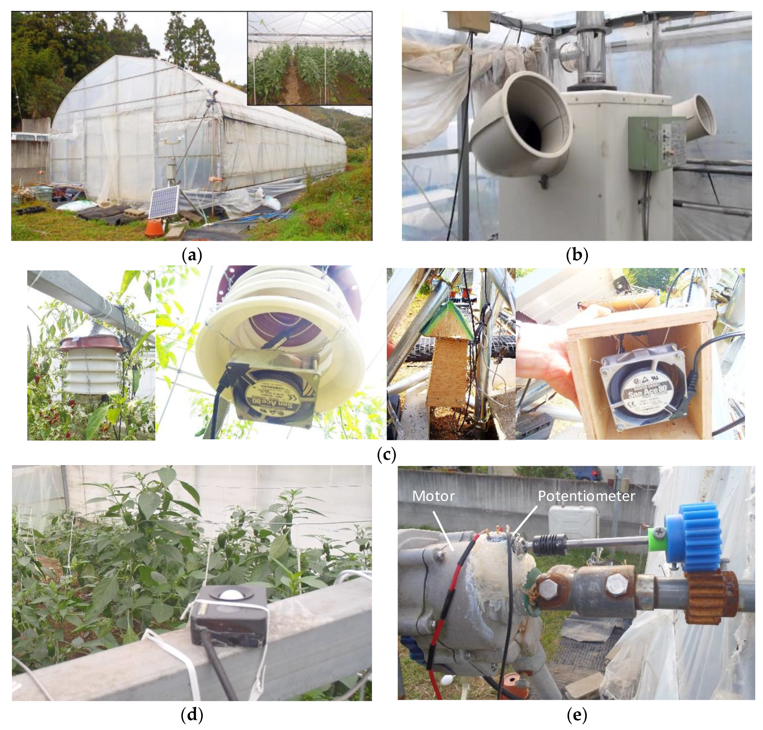
2.1. Overview of the Winter Greenhouse Measurement Environment

Measurements were taken at a greenhouse facility for green peppers in Geisei Village, Aki-gun, Kochi Prefecture, Japan, from 6 December to 12 January 2019 after planting on 27 August 2018. As shown in Figure 1a, the greenhouse was a north–south building with a width, height, and depth of 5.5 m, 16 m, and 3.4 m, respectively; a semi-cylindrical shaped roof; and a double-layer structure with an outer lining (PO film) and inner lining (plastic). The greenhouse contained 30 plants in three rows (10 plants per row). The planting density was 1.6 m between rows and 70 cm between plants. Irrigation tubes were placed at the base of each plant. The timer valves were opened 4 times during the day for 30 min each. When the air temperature in the greenhouse reduced below 15 °C, the boiler shown in Figure 1b was switched on. The optimum daytime temperature for growing peppers is 27–28 °C. Therefore, a wind-up skylight automatic opening/closing device simultaneously opened and closed the inner and outer windows with a control cycle of 90 s at a window-opening volume proportional to the difference above the target value of 28 °C. The air temperature sensors of the boiler and window device were mounted independently at a height of 150 cm at the centre of the greenhouse. This greenhouse is a typical small-scale Japanese house without a humidifier that regulates the internal environment during the day through natural ventilation.
A GRAPHTEC GL100 data logger was installed in the greenhouse to acquire data from temperature and humidity sensors inside and outside the greenhouse (Figure 1c), an illumination sensor inside the greenhouse (Figure 1d), and a voltage sensor reading the window opening (Figure 1e) with a sampling period of 1 min. Temperature and humidity sensors inside and outside the greenhouse were placed in the ventilation tubes to prevent solar radiation. Forced ventilation was provided using an AC fan. Temperature and humidity sensors were placed inside the greenhouse at a height of 150 cm at the centre of the greenhouse. The temperature and humidity sensors outside the greenhouse was placed at a height of 50 cm in front of the greenhouse entrance. An illumination sensor was installed at a height of 180 cm in the middle of the greenhouse to prevent overshadowing by the green pepper colonies. The voltage sensor measured the window opening from 0% to 100% of the voltage of the potentiometer, which output 0–5 V at 10 revolutions. The roll-up motor for this greenhouse was a DC 24 V, 48 W, 4.5 rpm type commonly used in Japanese greenhouse cultivation. The vertical width of the window in this greenhouse was approximately 1 m, and the motor could fully open or close the window within a sample period of 1 min.

2.2. HD Calculation Formula

HD (g/m3) is the difference between saturated water vapour (g/m3) and absolute humidity (g/m3). This is an indicator of the room available for water vapour in the air. The appropriate HD value for institutional cultivation falls within 3–6 g/m3. This process promotes plant growth through photosynthesis. HD (g/m3), water vapour saturation c (g/m3), and water vapour saturation pressure e (hPa) at air temperature T (°C) and relative humidity R (%) can be expressed as follows:
H D = c × 100 R 100 ,             c = 217 × e T + 273.2 ,     e = 6.1078 × 10   7.5 T T + 237.3
The saturated water vapour pressure was calculated using the Tetens approximation. This implies that HD can be calculated using T and R .

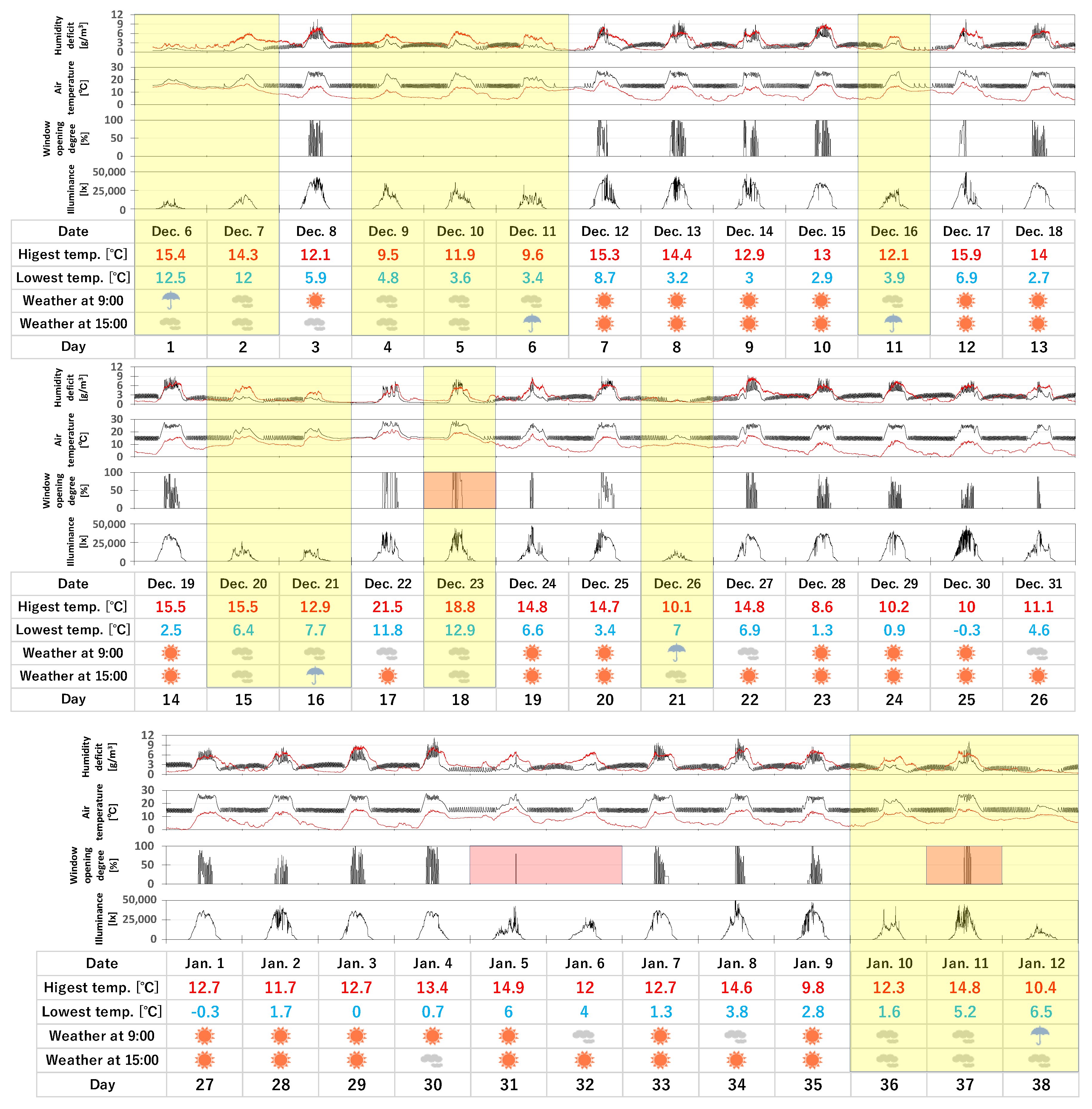
2.3. Environmental Measurement Data and Weather Information

We obtained environmental measurement data in the greenhouse from 06:00 on 6 December 2018 to 24:00 on 12 January 2019. Daily weather information for Kochi Prefecture is shown in Figure 2. Outside the greenhouse, the minimum temperature exceeded 10 °C, and the maximum temperature was approximately 20 °C on certain days. However, during the cold season, the minimum temperature was approximately 0 °C, and the maximum temperature reduced to approximately 10 °C. This indicated typical late-autumn to winter temperature variations. In the greenhouse, the air temperature was controlled to at least 15 °C at night (primarily from 16:00 to 8:00) using a boiler and at most 28 °C during the day (primarily from 8:00 to 16:00) using automatic window openers. During boiler operation, the air temperature in the greenhouse exhibited constant variations within a range owing to the intermittent switching of the boiler on and off. The boiler operated almost every night during winter. The inside HD was marginally lower than the outside HD. However, it exceeded 6 g/m3 on certain days. This may have hindered the effective growth of the peppers. On rainy and cloudy days (highlighted in yellow), windows were typically closed. However, the days highlighted in red were those when the illumination was high and the windows were automatically opened and closed during the day, notwithstanding cloudy weather. Sunny days not indicated in yellow are the days when the windows were opened and closed during the day owing to the higher temperatures in the greenhouses. However, the days indicated in red were those when, notwithstanding sunny weather, the illumination level was low and few window-opening/-closing events occurred. The results demonstrated a constant relationship between weather conditions and window opening during the winter months. However, there were certain exceptions.

3. Greenhouse HD and Air Temperature Model

3.1. Numerical Model Overview

A linear state-space model of the discrete-time system was set as follows:
x k + 1 = A x k + B d k u k y k = C x k    
where d is the measured disturbance input vector; u is the control input; y is the output vector; and x is the state variable. We set the input and output data as follows:
d = H D o T o L X i T , u = W , y = H D i T i T
where H D o is the outside HD (g/m3), T o is the outside air temperature (°C), L X i is the inside illuminance (lx), W is the window-opening degree (%), H D i is the inside HD (g/m3), and T i is the inside air temperature (°C). The input/output data are displacement data where the reference values for HD, illumination, and window opening are 0 and that for air temperature is 15 °C. (A boiler setting temperature of 15 °C was the actual minimum temperature in the greenhouses.) We set the order of the state variable x to six without introducing a delay time and constructed a sixth-order numerical model from the input–output data in (3) by obtaining matrices A , B , and C using the subspace method (N4SID) [30]. In model evaluation, we used the root mean square error (RMSE) as follows:
R M S E = 1 N k = 1 N y k y ^ ( k ) 2
where y is the measured value; y ^ is the model output value; k is the number of steps per sampling period; and N is the number of data points.
The fit rate is a widely used model evaluation value in the field of system identification. It is expressed as follows:
F i t   r a t e [ % ] = 1 k = 1 N y k y ^ ( k ) 2 k = 1 N y k y ¯ 2 · 100
where y ¯ is the mean value of measured y . The fit rate was RMSE-normalised using the standard deviation of the actual measured values. Therefore, the smaller the daily swing (maximum–minimum) of the output values, the lower the fit rate. Even if the RMSE were identical in the evaluation of the model for rainy and sunny days, the fit rate would be lower on rainy–cloudy days because the amplitudes of the temperature and HD in the greenhouse were likely to be smaller than those on sunny days. Significant variations in the evaluation of the model depending on the weather can be prevented by using the RMSE value rather than the fit rate.

3.2. Model Construction

The model required the dynamic response of the greenhouse HD and air temperature to window opening and closing during the day, as used in the MPC controller with window opening. Therefore, the model did not require the inclusion of data during the night (approximately 16:00–8:00), when the boiler was running and the windows were closed. In addition, as the air temperature in greenhouses does not increase on rainy and cloudy days and windows are generally closed, the model can be developed separately for sunny and rainy–cloudy days. In the future, these models could be used differently for weather forecasts. Based on this, models were constructed using datasets from which four periods were extracted: (1) nighttime and daytime, (2) daytime, (3) sunny daytime, and (4) rainy–cloudy daytime. The modelling period was 28 days, from days 4 to 31, as shown in Figure 2. Nighttime ranged from 16:00 to 8:00 the following day, and daytime from 8:00 to 16:00. Previous weather conditions were also recorded.
Figure 3 shows the measured and model output values for a sampling period of 1 min for the data periods used in the modelling of (1) 28 nights and days, (2) 28 days during the day, (3) 20 days during the day, and (4) 8 days during the day. Overall, the model output values closely match the measured values. However, differences were observed in the HD and air temperature at night in model (1) and in the air temperature during sunny days in models (1)–(3). However, the measured values at night had a large fluctuation range owing to the boiler operation, whereas the model output values captured the average of the measured values and appeared to be optimised. With regard to temperature errors, the daytime temperatures on days 17 and 18 had the largest errors, and the model output values were approximately 4 °C lower than the measured values. The RMSE for the entire modelling period ranged from 0.29 to 0.57 g/m3 for HD and from 0.81 to 1.58 °C for air temperature. The increasing order of the RMSEs for the models was (4) < (2) < (1) < (3) for HD and (4) < (1) < (2) < (3) for air temperature. The RMSE of (4) was smaller for both the HD and air temperature, whereas that of (3) was larger. The difference between models (4) and (3) can be considered as the difference between the small and moderate fluctuations in greenhouse illumination and window opening during the daytime (4) and the large and intense fluctuations during the daytime (3). The RMSEs of the HD and air temperatures tended to be small when the fluctuations in the illumination and window opening were small and moderate, respectively. Meanwhile, the RMSEs of the HD and air temperature tended to be large when the fluctuations in illumination and window opening were large and intense.

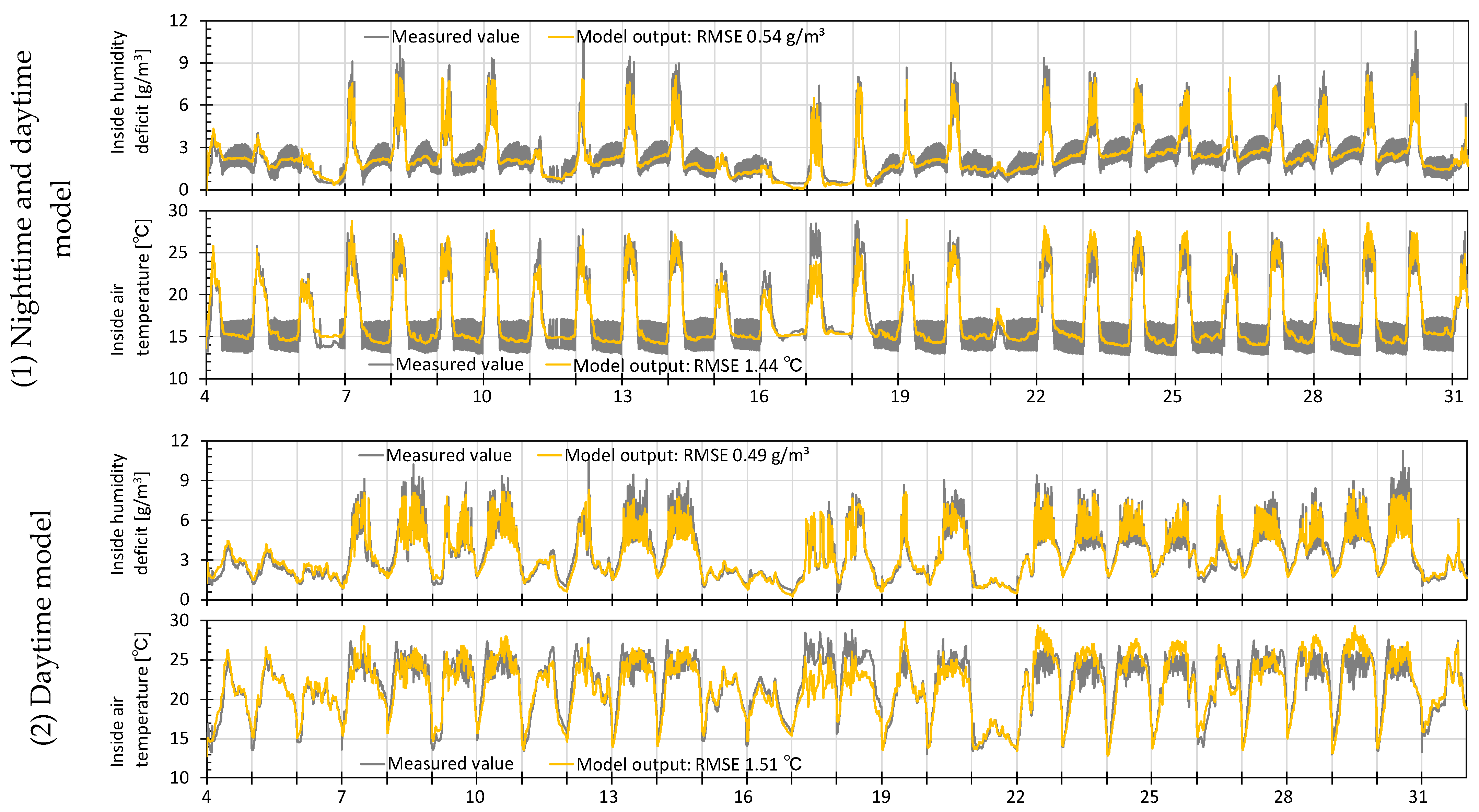
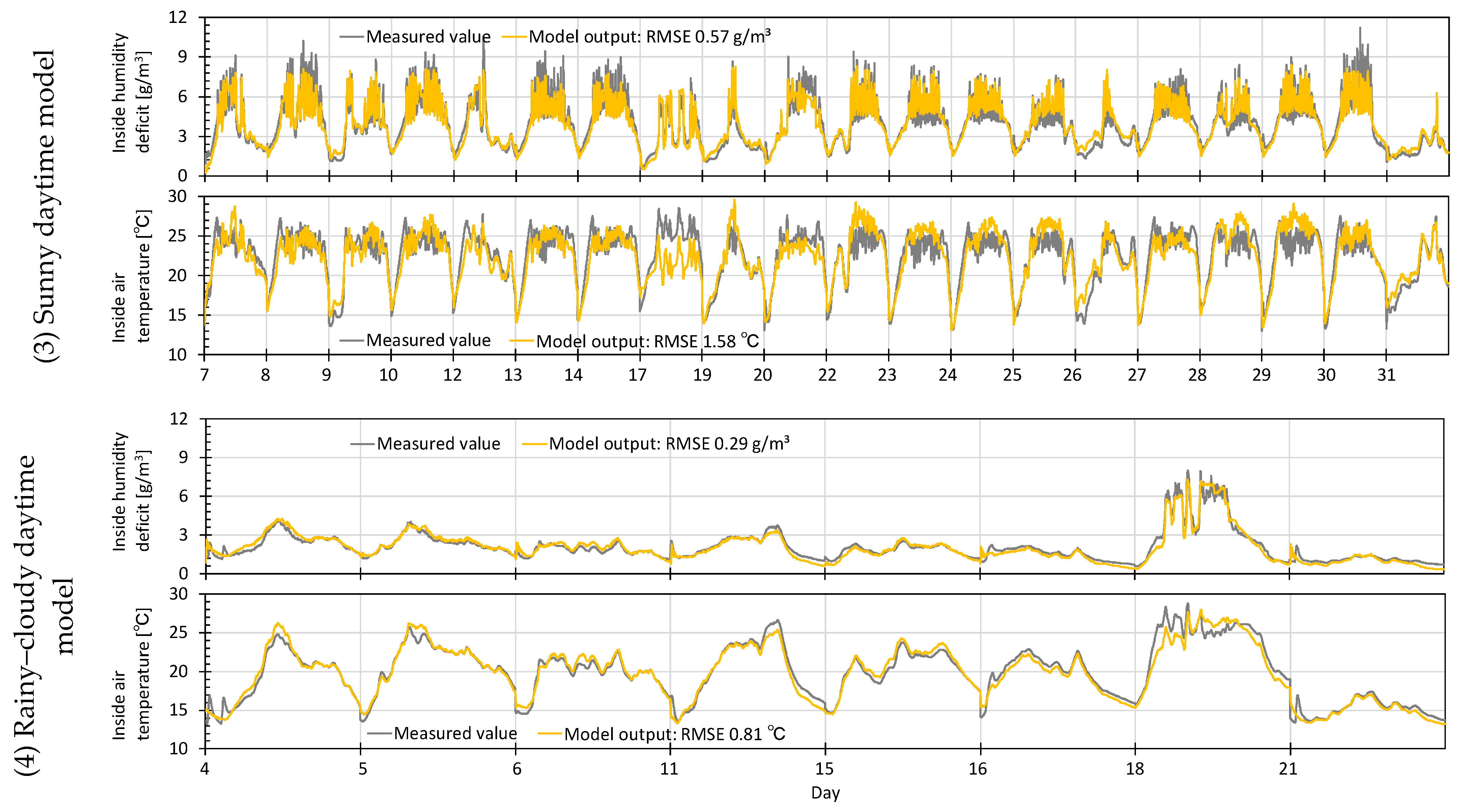
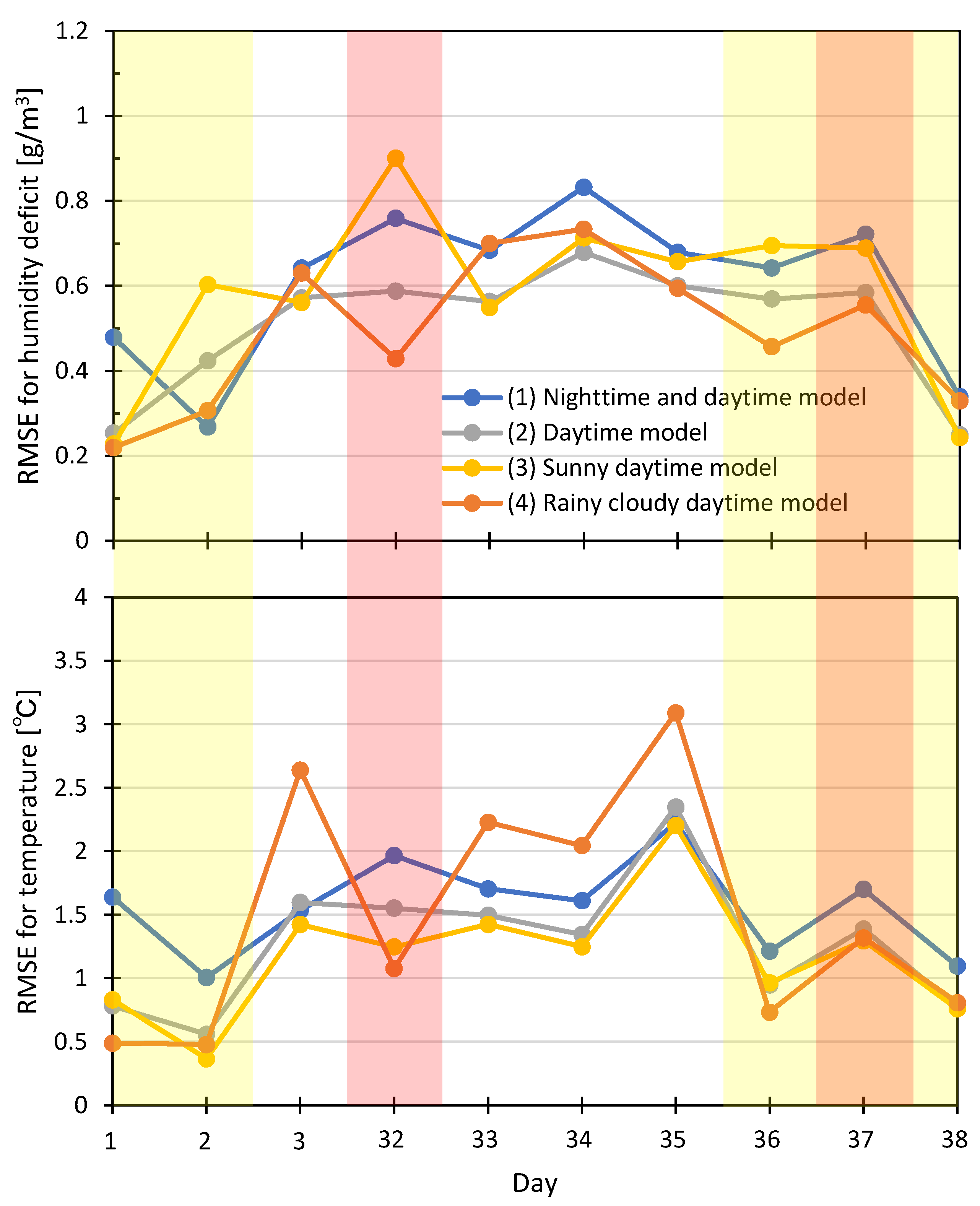
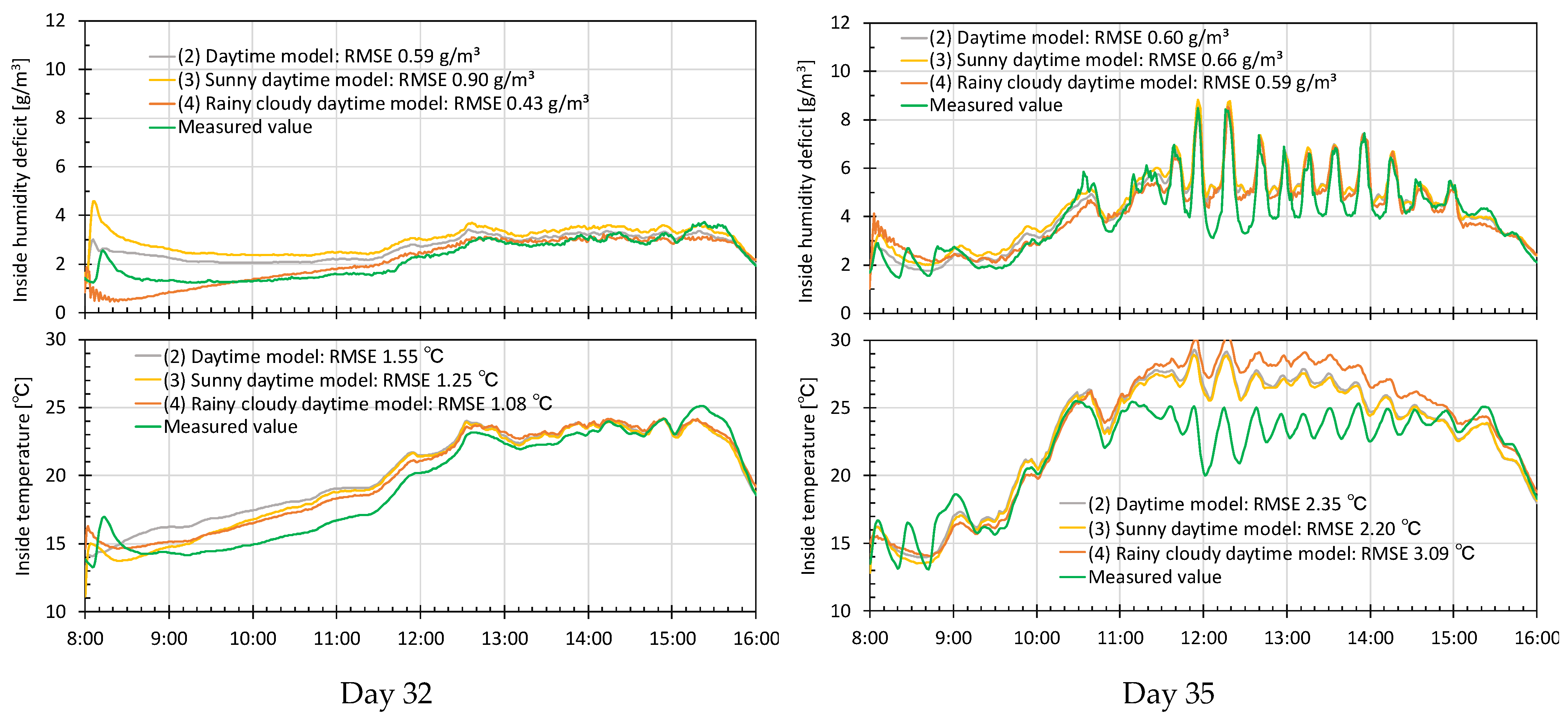
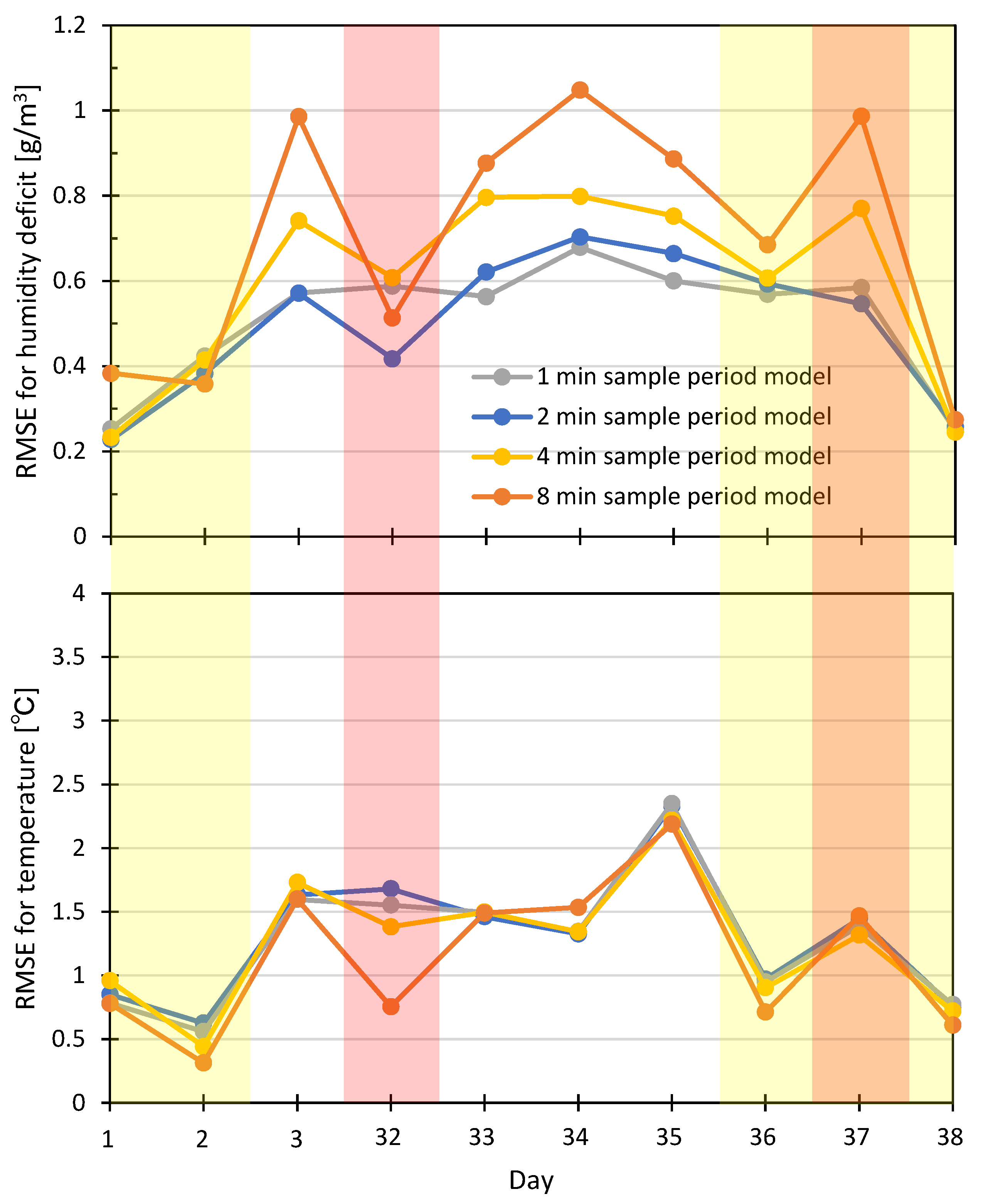
3.3. Model Evaluation

We set the 10 days that were not used for model construction (days 1–3 and 31–38 in Figure 2) as the model evaluation period. Therefore, the weather was equalised: five sunny days out of the ten evaluation periods (only one day where the window was closed) and five rainy–cloudy days (only one day where the window was open). The daily RMSEs of the measured and model outputs for the period from 8:00 to 16:00 during the daytime in the model evaluation period are shown in Figure 4. Overall, the RMSEs for the HD and air temperature tended to be higher on sunny days than on cloudy or rainy days because the HD and air temperature fluctuations in the greenhouses were large and intense on sunny days. The RMSEs for HD and air temperature tended to be minimised when model (3) was used on sunny days and model (4) was used on rainy–cloudy days. For sunny day 32 and rainy–cloudy day 37, where the window movement was inappropriate for the weather, the RMSE of model (3) for day 32 was larger, whereas that of model (4) for day 37 was unaffected. In (3) and (4), days 18 and 31 (which were subjected to identical conditions) were incorporated into the modelling period. However, for model (3), the proportion was one-twentieth of the total period, and for model (4), it was one-eighth of the total period. This may explain the difference in the RMSE influences between (3) and (4). When models (3) and (4) were used separately for different weather conditions, the RMSE of models (1)–(4) tended to be the highest for model (1). The RMSE of model (2) tended to be intermediate between those of models (3) and (4). Overall, the RMSE was less than 1 g/m3 for the HD difference and within 2 °C for the temperature, with certain values being approximately 3 °C. The required measurement accuracy in the field is less than 0.5 g/m3 for HD and 0.5 °C for temperature. However, this model was intended to be used to predict HD and temperature in a greenhouse 10–20 min in advance. When using the model, the predicted values are calculated by considering the difference between the current measured values and the model output values so that the model can sufficiently achieve predictions with an accuracy of below 0.5 g/m3 and 0.5 °C. In particular, because MPC considers the difference between the current measured value and model output value while modifying the predicted value from time to time, a model with an error of approximately 1 g/m3 in HD difference and 1–2 °C in temperature throughout the day can be used effectively.
The daily model outputs for days 32 and 35, when the RMSE was at its maximum, are shown in Figure 5. The large 20 min cycles of observable peaks and dips in the measured HD and air temperature values were due to the effect of the boiler at 8:00–9:00 on days 32 and 35 and that of the automatic window opener at 10:30–15:10 on day 35. On day 32, which was sunny, the RMSE for the HD was the largest for model (3), whereas those for the HD and temperature were the smallest for model (4) because day 32 was sunny and had low illumination. Moreover, the window was not open, which is typical of model (4). In contrast, model (2) included a good balance of days when windows were opened and closed during the modelling period, and the RMSE remained small even for days with a typical pattern of rainy and cloudy weather, notwithstanding sunny days. For day 35 (sunny day), the RMSE of the air temperature was above 2 °C for all the models. On this day, the maximum temperature was below 10 °C, and the temperature difference between the inside and outside of the greenhouse was large (10–15 °C). Therefore, the effect of opening the window to reduce the air temperature inside the greenhouse was greater than normal. Furthermore, the model output values do not match the measured values.
Table 1 presents the average evaluation results for each model. Weather-specific models (3) and (4) were applied to sunny and rainy–cloudy days, respectively, according to the actual weather conditions. The average RMSE values for all the models were sufficiently accurate (<0.60 g/m3 for HD and <1.57 °C for temperature). For HD, the RMSE of model (2) was 0.51 g/m3. For temperature, the RMSE of models (3) and (4) was 1.14 °C. The weather-specific model did not achieve high accuracy for HD because the RMSE of model (3) for day 32 was large. However, the RMSE of model (4) was small for both HD and air temperature. This indicates that the weather-specific model evaluation may be more effective if (3) and (4) are used appropriately.

4. Model Predictive Control

In this section, we describe the development of an MPC controller based on the HD and temperature models discussed in Section 3. MPC simulations were conducted using actual measurements during the model evaluation period to verify the performance of the MPC controller.

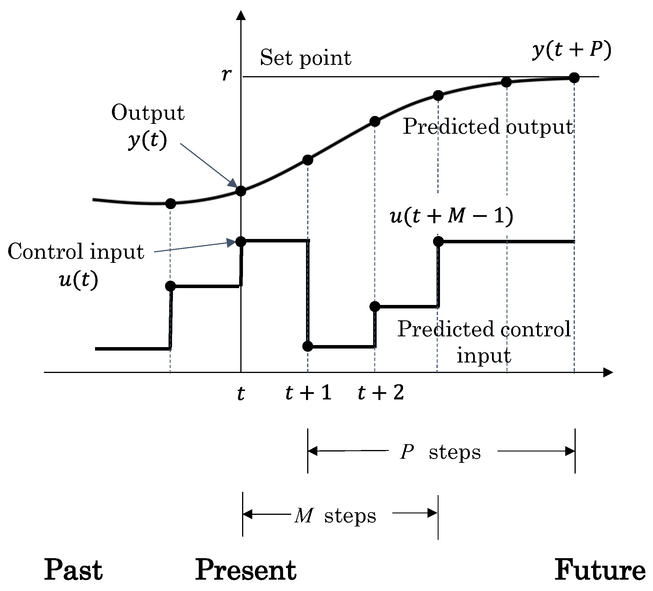
4.1. Algorithms for Model Predictive Control

MPC is a control method that performs optimisation using a model to predict the response that will occur in the future for a certain period at each time step. A conceptual diagram of the MPC is shown in Figure 6. This algorithm is described elsewhere [31]. The predicted interval of P steps is called the prediction horizon. The controlled interval of M steps is called the control horizon.
  • The control input trajectories of u t , u t + 1 , ,   u ( t + M 1 ) are calculated such that the predicted output y in the section of P steps in [ t + 1 , t + P ] is closest to the target value r , and the control input u in the section of M steps in [ t , t + M 1 ] is the minimum.
  • The first step of the calculated control input trajectory u t is used as the input for the next step until sampling time t + 1 .
  • Time t is advanced by one step, and the procedure returns to step I.
MPC was performed using the moving horizon method, which repeats steps I–III at each sampling timepoint. The cost function used in step I is
J = k = 1 P r y ( t + k ) T Q r y ( t + k ) + u ( t + k ) T R u ( t + k )
where Q is the weight of the error vector and R is the weight of the control input u .  We consider the optimisation problem of the control system represented by Equation (2) using Equation (6). The constraints were set as 0 u 100 (%) and y 1 6 (g/m3). Equation (2) represents the greenhouse system during the daytime from 8:00 to 16:00 ( t = 0   t o   480   m i n ). At 8:00, the initial states in Equation (2) within the MPC controller are set as x 0 = o ,     y 0 = o (where temperature y 2 is the displacement value from 15 °C). The target values were set as r = [ 4.5 ; 11 ] (with the target temperature r 2 being the displacement value from 15 °C). The MPC controller predicts the output y t + 1 ~ t + P up to P steps ahead using the measured disturbance d t and the control input trajectory u t ~ t + M 1 . (In practice, the predicted output y t + 1 ~ t + P considers the difference between the actual measurement at time t and the model output.) The MPC controller repeats steps I–III from 8:00 to 16:00.

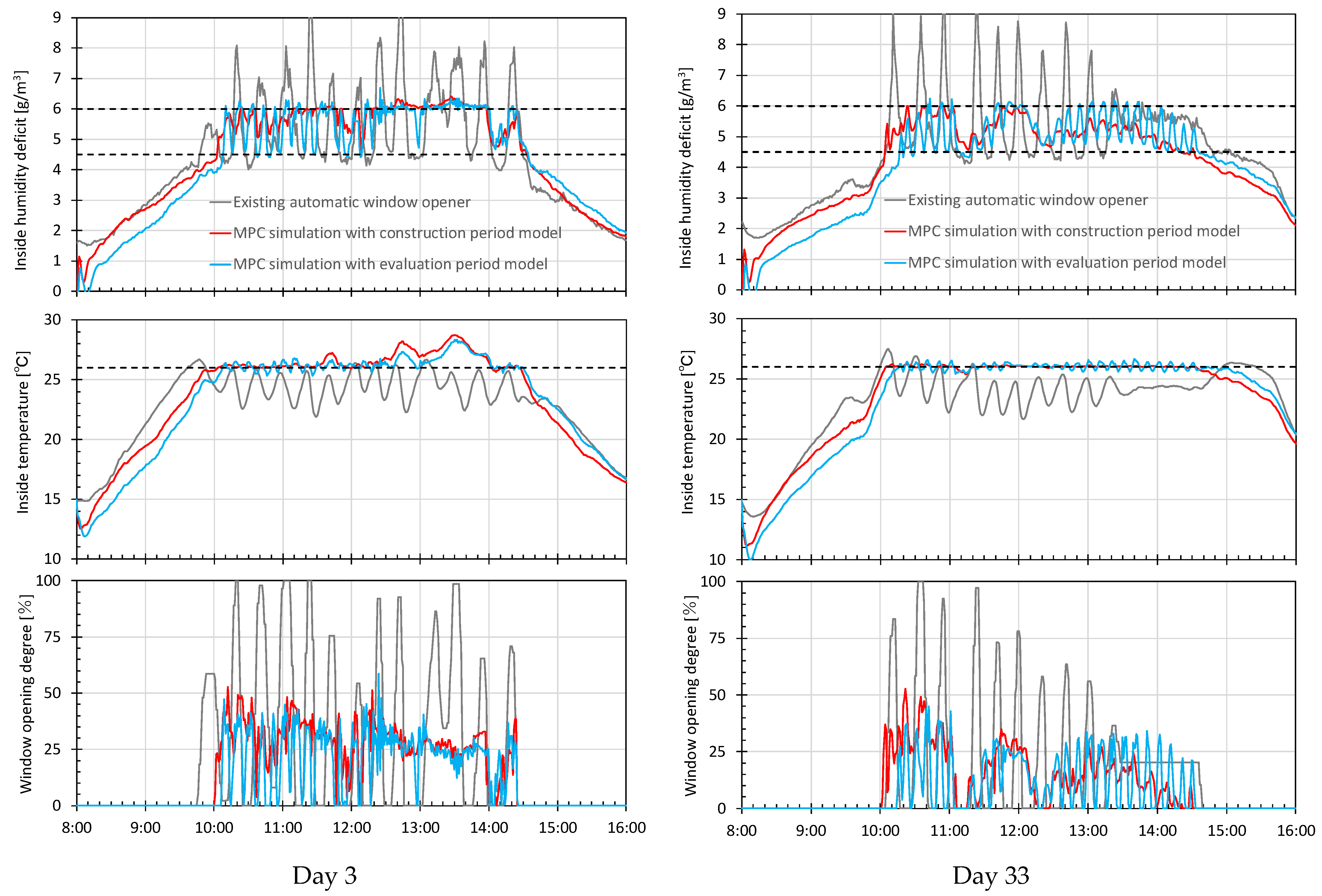
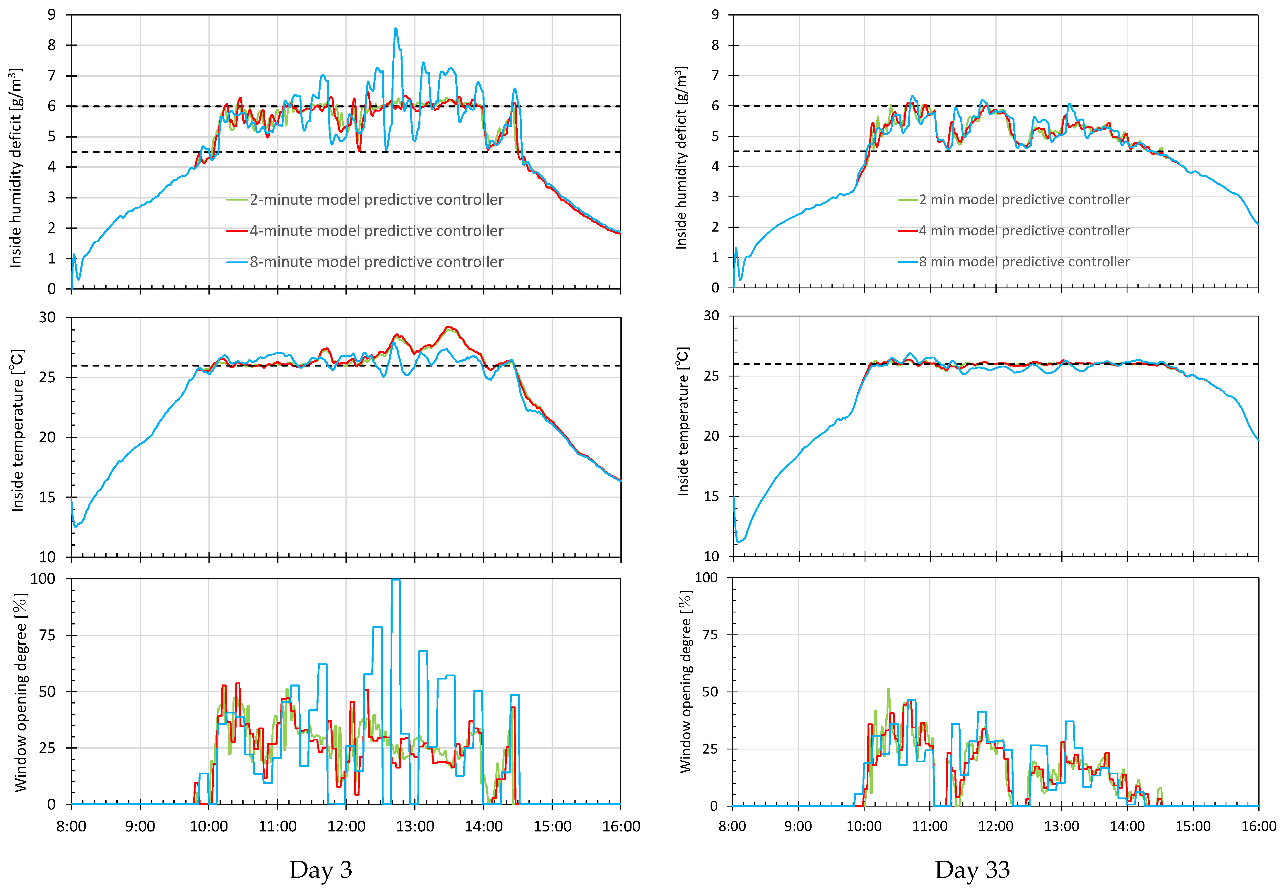
4.2. Model Predictive Control Simulation

The MPC controller was developed using model (2). (Here, we selected model (2) because the RMSEs of the HD and air temperature were relatively small. However, if the RMSE of the weather-specific models (3) or (4) is small, that model is preferable.) The greenhouse model used in the simulation was model (2), with a sampling period of 1 min obtained during the model construction period. To consider the influence of modelling errors in the MPC controller, we constructed a model similar to model (2) for the evaluation period and conducted simulations. The disturbance inputs ( H D o , T o , and L X i in Equation (3) in Section 3.1) from 8:00 to 16:00 during the evaluation period were input into the greenhouse model to evaluate whether the MPC controller could calculate the appropriate control input ( W ) and control the output ( H D i and T i ). For the controller design, the target temperature in the greenhouse was set at 26 °C, and the target HD was set at 4.5 g/m3 with an upper limit of 6 g/m3. The optimum temperature for growing green peppers is 27–28 °C. However, the existing window-opening/-closing system practically controlled the air temperature in the greenhouse to at most 26 °C. Therefore, we used a target temperature of 26 °C to facilitate comparison. The delay until the temperature in the greenhouse varied because of the opening and closing of the windows was approximately 5 min, whereas that for HD was almost zero. Therefore, for the MPC controller with a sampling period of 1 min, the prediction horizon was set to P = 16 (16 min). This was three times the air temperature delay time. The control horizon is generally set to approximately three steps to reduce the computational cost. However, to suppress the movement of the window openings for a longer period, we set it to M = 8 (8 min). This was half of the predicted horizon. The weight R was set to R = 1 . The larger the weight, the more the window-opening and window-closing movements are suppressed. However, the operability of the controlled variable was reduced by opening the windows. The weight was set to Q = [ 1   0 ; 0   100 ] , and the sensitivity of the temperature error was considerably higher than that of the HD error. The operability of the air temperature by opening windows in the greenhouses was higher than in the HD. On a typical winter day with solar radiation, increasing or decreasing the window opening can regulate the rate of variation in the air temperature in a greenhouse. However, this would cause an abrupt increase and decrease in the HD. Because the HD is proportional to the increase or decrease in air temperature, if the control of air temperature is prioritised, the HD can be increased or decreased by increasing or decreasing the air temperature. However, if HD control is prioritised, the window tends to close to prevent an abrupt increase in the HD. Moreover, closing the window leads to an increase in temperature. This, in turn, causes the HD to increase.
We performed MPC simulations for an evaluation period of 10 days. On days when the daytime illuminance was less than 25,000 lx and the window of the existing window opener was not open (days 1, 2, 32, 36, and 38), the window of the MPC controller was not opened. On days when the daytime illumination was less than 25,000 lx and the window was not opened with the existing window opener (days 1, 2, 32, 36, and 38), the window was not opened with the MPC controller. However, on days when the daytime illumination was higher than 25,000 lx and the window was opened with the existing window opener (days 3, 33, 34, 35, and 37), it was opened with the MPC controller. Examples of the daily variations from the MPC simulations (days 3 and 33) are shown in Figure 7. ‘MPC simulation with evaluation period model’ was displayed to consider the influence of modelling errors in the MPC controller. The existing window openers exhibited a large hunting phenomenon with an HD of approximately 4 g/m3 and a temperature of approximately 4 °C. On ten occasions, the HD exceeded 6 g/m3 and was higher than 6.5 g/m3. However, the MPC window opener suppressed large hunting in both cases and achieved control with a maximum HD of 6.5 g/m3. On day 3, the MPC controller achieved a control where the target value of 26 °C was generally maintained. However, the HD in the greenhouse did not increase, even when the air temperature exceeded the target value, similar to that from 12:20 to 14:00 (when the HD in the greenhouse exceeded 6 g/m3). Similar control effects were observed on days 3, 34, and 35, when daytime HD outside the greenhouse exceeded 6 g/m3. The MPC controller on day 33, during which the daytime outside the greenhouse HD was below 6 g/m3, achieved a control below 6 g/m3 (close to the target value of 4.5 g/m3). Meanwhile, the target temperature of 26 °C was typically maintained. A similar effect was observed on day 37, when the daytime outside the greenhouse HD was less than 6 g/m3. The influence of modelling errors in the MPC controller appeared in the frequent corrective actions of window opening, causing the temperature, especially the HD, to oscillate. However, the control objectives could still be achieved. Here, we considered the temperature and humidity oscillations that occurred when applying the MPC controller based on the construction period model to the evaluation period model. First, the MPC controller prioritised temperature control by setting a significant weight on the temperature error. Additionally, the evaluation period model had approximately 1.5 times the effect of window opening on the inside temperature compared to the construction period model. The MPC controller, which was based on the construction period model, opened and closed the window early, bringing the predicted temperature closer to the target value. However, as the temperature increased significantly higher than predicted, this controller initiated early corrective actions by opening and closing windows in the opposite direction. This repetitive process resulted in a weak hunting of about 1 °C in temperature. Moreover, as the delay time from HD to window opening was short (1 min), HD exhibited significant hunting, depending on the window opening. The difference in the effect of window opening, which is thought to arise from the difference in temperature between the inside and outside of the greenhouse, can be considered as the cause of this phenomenon. While this greenhouse model assumes a linear approximation model where the window opening and the outside temperature independently affect the inside temperature, the reality is a nonlinear model in which the temperature difference between the inside and outside of the greenhouse affects the inside temperature through the window opening. This phenomenon is fundamentally attributed to the influence of modelling errors owing to the linear approximation.

4.3. Effects of the Sampling Period on the Model Predictive Controller

The MPC controller outputs the degree of window opening every minute. This is because it was based on a model with a sampling period of 1 min. In practical applications, if the window opener is operated every minute, the motor’s power consumption increases, and its life is shortened. Therefore, we consider an MPC controller that uses a daytime model with an extended sampling period for model construction.
First, the daytime model obtained in Section 3, with a sampling period of 1 min, was reconstructed with sampling periods of 2, 4, and 8 min, and the model accuracies were compared. The results of the comparative evaluation of the models with sampling periods of 1, 2, 4, and 8 min are shown in Figure 8. For air temperature, the RMSEs of all the models showed negligible differences. The delay time for the window-opening degree with respect to air temperature was approximately 5 min. Therefore, even when the sampling period was increased to approximately 5 min, the difference between the model output and the measured values did not increase. By contrast, for the HD group, the RMSE increased on days when the window was open (days 3, 33, 34, 35, and 37), with a maximum model difference of 0.4 g/m3. The delay time for the window-opening degree of the HD was approximately 1 min. Therefore, increasing the sampling period to more than 1 min resulted in larger discrepancies between the model output and the measured values.
Here, we constructed MPC controllers with sampling periods of 2, 4, and 8 min, a prediction horizon of 16 min, and a control horizon of 8 min, without modifying the cost function weights. Control simulations were performed over a 10-day evaluation period with a model sampling period of 1 min. Examples of daily variations from the MPC simulations (days 3 and 33) are shown in Figure 9. MPC with a longer sampling period resulted in a longer time interval for the window to open and close. This reduced the frequency of the window movement. The MPC controller with sampling periods of 2 min and 4 min exhibited a performance almost equal to that of the MPC controller with a sampling period of 1 min on days 3, 33, 34, 35, and 37. The MPC controller with sampling periods of 2 min and 4 min exhibited a performance almost equal to that of the MPC controller with a sampling period of 1 min on days 3, 33, 34, 35, and 37. In contrast, the MPC controller with a sampling period of 8 min performed similarly to the MPC controller with sampling periods of 2 and 4 min on day 33 (when the illuminance variation during the day was marginal). However, on days 3, 34, 35, and 37, when the variation in illuminance was severe, it exceeded 6 g/m3 several times a day, reaching at least 6.5 g/m3. The performance of the MPC controller with a sampling period of 8 min was lower than that of the other MPC controllers with shorter sampling periods. Finally, the MPC controller with a sampling period of 4 min was the most energy-efficient controller that could be operated with assured control performance.

5. Considerations

Wind speed and direction are crucial parameters in modelling based on window operations. However, during the winter season, greenhouses typically close all openings except for roof vents to prevent drafts. In this study, we constructed a model with a certain level of accuracy without considering wind speed and direction. In the future, to improve model accuracy, we need to investigate the influence of wind speed and direction. During the modelling period, window opening as a control input varied from 0% (fully closed) to 100% (fully open). However, in the absence of 100% fully open conditions during the modelling period, the model may not represent the maximum influence of window openings on the greenhouse environment. The input–output values of the model were the displacement data from the reference values. However, the measured values at 8:00 h each day in both the modelling and evaluation periods were relatively close to the reference values except for the air temperature outside the greenhouse. Therefore, the accuracy of the model was improved. However, variations in seasonality and boiler shutdown times may affect the model performance. Various models are evaluated in this study. However, because the behaviour of the input–output values varies significantly depending on the weather conditions, it is more effective to use different weather-specific models depending on the weather forecast. Meanwhile, the accuracy of the weather-specific models deteriorates if exceptional days (such as the typical ‘window will not open’ day on a rainy day) occur, notwithstanding a sunny day. In such scenarios, artificially inserting more exceptional days into the modelling period is likely to result in higher accuracy, even for weather-specific models. MPC does not need to be performed by opening windows on typical rainy–cloudy days or exceptionally sunny days when windows are closed all day. In contrast, an MPC controller using window opening can be considered to perform well as long as the model accuracy is sufficiently high for typical sunny days or exceptionally rainy–cloudy days when the windows are open.
Although not presented in this paper, the performance of the MPC with a sample time of 1 min was not improved significantly by the variation of the weights Q and R of the evaluation function and the prediction horizon P and control horizon M from the present settings or by the introduction of a weight R u for the rate of variation u of the control input in the cost function in Equation (6). However, the MPC controller with a sampling period longer than 1 min during model construction reduced the frequency of window movements while maintaining control performance. Meanwhile, when the sampling period exceeded 5 min, which was the time delay between the window opening and air temperature, the control performance deteriorated. Therefore, the sampling period was maintained at 5 min. However, considering that the initial set value of the control cycle in existing window-opening/-closing systems is 1.5 min and the set limit is 3 min and 20 s, a control cycle of 2–4 min is considered practical and sufficient to reduce the load on the motor. With this 2–4 min control cycle, concerns regarding HD exceeding 6 g/m3 during the control cycle with a fixed window opening can be addressed through the output prediction of the MPC. The effect of the window is essentially a trade-off between ‘closing it would suppress the HD spike but not the air temperature increase’ and ‘opening it would reduce the air temperature but cause the HD to spike’. However, MPC exhibited an optimal solution to this trade-off.
In this study, simulation experiments were conducted under conditions in which the controller model matched the model to which the control signal was applied. Simulation experiments using different models were discussed in references [27,28]. In this system, it was verified that the degradation of the control performance owing to errors between the model in the controller and the applied model is marginal and can be compensated for by the sequential correction operation of the MPC. The temperature and HD inside the greenhouse exhibited significant daily variations owing to external environmental influences and short-term variations of approximately 10 min owing to window opening/closing and sunlight. Although this MPC with window opening/closing cannot significantly alter the daily trend, it can locally maintain the temperature and HD at appropriate values. Thus, the application of PID control is more convenient. However, it requires effective consideration of the switching rules for temperature and HD control as well as adaptation to variations in external conditions. This poses optimisation challenges. The object of ‘controlling temperature and HD through window opening while adapting to external conditions’ is well-suited for multi-input and multi-output control. In particular, the MPC adopts proactive measures to prevent an increase in the HD inside greenhouses.

6. Conclusions

During winter daytime in a greenhouse environment, it is necessary to perform window-opening and -closing controls to maintain the target temperature while ensuring that the HD ranges from 3 to 6 g/m3. However, few practical studies on MPC for controlling the temperature and HD have been conducted. The input and output values of the model depend significantly on the daily weather conditions. Therefore, the accuracy of a model can be enhanced by selecting weather-specific models based on weather forecasts. In addition, conventional MPC controllers encounter challenges in terms of control inputs, such as window-opening motors, which vary with each sampling period in the model. This increased frequency during operation results in higher power consumption, a shortened lifespan, and operational issues. To address these challenges, in this study, we constructed models using the subspace method (N4SID) to capture environmental data inside and outside a winter greenhouse, considering the effects of weather and the sampling period. Furthermore, we performed the MPC of HD and air temperature measurements in greenhouses.
First, four models were constructed over a 28-day modelling period: (1) nighttime and daytime models, (2) daytime models, (3) sunny daytime models, and (4) rainy–cloudy daytime models. The average RMSE values from 8:00 to 16:00 over a 10-day modelling evaluation period were examined. The results show that model (2) can operate with an RMSE of 0.51 g/m3 for HD and that models (3) and (4) (weather-specific models) can operate with an RMSE of 1.14 °C for air temperature. In terms of HD, weather-specific models (3) and (4) did not achieve the lowest RMSE. This is because sunny days in the evaluation period included days with low illumination (similar to rainy and cloudy days), which yielded an increased RMSE for (3). A viable solution is to insert additional exceptional days into the model construction period. This approach can improve the accuracy of weather-specific models based on weather forecasts.
Subsequently, we developed MPC controllers from the four models with sampling periods of 1, 2, 4, and 8 min and compared their performances over the model evaluation period. The MPC controller with a sampling period of 4 min was the most energy-efficient operational controller. It achieved HD control below 6 g/m3 and close to the target value of 4.5 g/m3 while maintaining the target temperature value of 26 °C. Considering that the control period of a conventional greenhouse temperature management window-opening device is limited to 3 min and 20 s, implementing this MPC controller with a 4 min control period on the same window-opening device can alleviate the load on the window-opening motor and enable the simultaneous management of temperature and HD without being concerned regarding overshoot. This method is not limited to greenhouse control and has applications in other fields.

Author Contributions

Conceptualization, S.N. and T.T.; methodology, S.N.; software, S.N.; validation, S.N.; formal analysis, S.N. and T.T.; investigation, S.N., T.T., R.K. and M.O.; resources, S.N., T.T., R.K. and M.O.; data curation, S.N.; writing—original draft preparation, S.N.; writing—review and editing, T.T.; visualization, S.N.; supervision, T.T.; project administration, S.N.; funding acquisition, S.N. and M.O. All authors have read and agreed to the published version of the manuscript.

Funding

This research was funded by JSPS KAKENHI (grant number 20K06332) and the Takahashi Industrial and Economic Research Foundation (grant number 13-003-328). The APC was funded by the National Institute of Technology (KOSEN), Japan.

Data Availability Statement

The data in this study are available on request from the corresponding author.

Acknowledgments

We are grateful to Koichi Oka of Kochi University of Technology, Shinsuke Kitamura, Principal of Kochi Prefectural Kochi Technical High School, and his mother, Yasuko Kitamura, for providing the greenhouse facilities. We express our deepest gratitude to the editor and reviewers for their comments that helped improve this paper.

Conflicts of Interest

The authors declare no conflicts of interest.

References

  1. Bailey, B.J.; Seginer, I. Optimum control of greenhouse. Acta Hortic. 1989, 245, 512–518. [Google Scholar] [CrossRef]
  2. Seginer, I. Optimal Greenhouse Temperature Trajectories for a Multi-State-Variable Tomato Model. In Proceedings of the IFAC Mathematical and Control Applications in Agriculture and Horticulture, Matsuyama, Japan, 30 September–3 October 1991. [Google Scholar]
  3. Stanghellini, C.; de Jong, T. A model of humidity and its applications in a greenhouse. Agric. For. Meteorol. 1995, 76, 129–148. [Google Scholar] [CrossRef]
  4. Nielsen, B.; Madsen, H. Identification of transfer functions for control of greenhouse air temperature. Agric. Eng. Res. 1995, 60, 25–34. [Google Scholar] [CrossRef]
  5. Nielsen, B.; Madsen, H. Predictive Control of air Temperature in Greenhouses. In Proceedings of the IFAC 13th Triennial World Congress, San Francisco, CA, USA, 30 June–5 July 1996. [Google Scholar]
  6. Sigrimis, N.; Rerras, N. A linear model for greenhouse control. Am. Soc. Agric. Biol. Eng. 1996, 39, 253–261. [Google Scholar] [CrossRef]
  7. Boaventura Cunha, J.; Couto, C.; Ruano, A.E. Real-time parameter estimation of dynamic temperature models for greenhouse environmental control. Control Eng. Pract. 1997, 5, 1473–1481. [Google Scholar] [CrossRef]
  8. Senent, J.S.; Martinez, M.A.; Blasco, X.; Sanchis, J. MIMO Predictive Control of Temperature and Humidity inside a Greenhouse using Simulated Annealing (SA) as Optimizer of a Multicriteria Index. In Proceedings of the 11th International Conference on Industrial and Engineering Applications of Artificial Intelligence and Expert Systems, Castellon, Spain, 1 June 1998. [Google Scholar]
  9. Van Straten, G.; van Willigenburg, G.; van Henten, E.; van Ooteghem, R. Optimal Control of Greenhouse Cultivation; CRC Press: Boca Raton, FL, USA, 2010; pp. 39–88. [Google Scholar]
  10. Rodríguez, F.; Berenguel, M.; Guzmán, J.L.; Ramírez-Arias, A. Modeling and Control of Greenhouse Crop Growth; Springer International Publishing: Berlin, Germany, 2015; pp. 1–96. [Google Scholar]
  11. Leyva, R.; Constán-Aguilar, C.; Sánchez-Rodríguez, E.; Romero-Gámez, M.; Soriano, T. Cooling systems in screenhouses: Effect on microclimate, productivity and plant response in a tomato crop. Biosyst. Eng. 2015, 129, 100–111. [Google Scholar] [CrossRef]
  12. Zhang, D.; Zhang, Z.; Li, J.; Chang, Y.; Du, Q.; Pan, T. Regulation of vapor pressure deficit by greenhouse micro-fog systems improved growth and productivity of tomato via enhancing photosynthesis during summer season. PLoS ONE 2015, 10, e0133919. [Google Scholar] [CrossRef] [PubMed]
  13. Zhang, D.; Du, Q.; Zhang, Z.; Jiao, X.; Song, X.; Li, J. Vapour pressure deficit control in relation to water transport and water productivity in greenhouse tomato production during summer. Sci. Rep. 2017, 7, 43461. [Google Scholar] [CrossRef]
  14. Koga, T.; Yamaguchi, K.; Iwata, H.; Kurimoto, I. Kriging interpolation evaluation of vapor pressure deficit in plant factory with solar light. J. Control Meas. Syst. Integr. 2020, 13, 131–137. [Google Scholar] [CrossRef]
  15. Takakura, T. Why control by vapor pressure deficit rather than relative humidity? Agric. Hortic. 2014, 89, 40–43. (In Japanese) [Google Scholar]
  16. Saito, A. The Guidebook of Climate Control for Greenhouse; Rural Culture Association Japan: Tokyo, Japan, 2015; pp. 32–37. (In Japanese) [Google Scholar]
  17. Akayama, N.; Arita, D.; Shimada, A.; Taniguchi, R.I. A Web Application for Visualizing Sensor Information in Farm Fields. In Proceedings of the 9th International Conference on Sensor Networks, Valletta, Malta, 28–29 February 2020. [Google Scholar]
  18. El Ghoumari, M.Y.; Tantau, H.-J.; Serrano, J. Non-linear constrained MPC: Real-time implementation of greenhouse air temperature control. Comput. Electron. Agric. 2005, 49, 345–356. [Google Scholar] [CrossRef]
  19. Frausto, H.U.; Pieters, J.G.; Deltour, J.M. Modelling greenhouse temperature by means of auto regressive models. Biosyst. Eng. 2003, 84, 147–157. [Google Scholar] [CrossRef]
  20. Frausto, H.U.; Pieters, J.G. Modeling greenhouse temperature using system identification by means of neural networks. Neurocomputing 2004, 56, 423–428. [Google Scholar] [CrossRef]
  21. Pawlowski, A.; Guzmán, J.L.; Rodríguez, F.; Berenguel, M.; Normey-Rico, J.E. Predictive Control with Disturbance Forecasting for Greenhouse Diurnal Temperature Control. In Proceedings of the 18th IFAC World Congress, Milano, Italy, 28 August–2 September 2011. [Google Scholar]
  22. Outanoute, M.; Selmani, A.; Guerbaoui, M.; Ed-dahhak, A.; Lachhab, A.; Bouchikhi, B. Predictive control algorithm using Laguerre functions for greenhouse temperature control. Int. J. Control Autom. 2018, 11, 11–20. [Google Scholar]
  23. Hamidane, H.; Faiz, S.E.; Guerbaoui, M.; Ed-Dahhak, A.; Lachhab, A.; Bouchikhi, B. Constrained discrete model predictive control of a greenhouse system temperature. Int. J. Electr. Comput. Eng. 2020, 11, 1223–1234. [Google Scholar] [CrossRef]
  24. Ito, K.; Tabei, T. Model predictive temperature and humidity control of greenhouse with ventilation. Procedia Comput. Sci. 2021, 192, 212–221. [Google Scholar] [CrossRef]
  25. Moufid, A.; Bennis, N.; Ramos-Fernandez, J.C.; Hani, S.E. Advanced constrained model predictive control of vapor pressure deficit in agricultural greenhouses. Int. J. Eng. Appl. 2022, 10, 363–374. [Google Scholar] [CrossRef]
  26. Nakayama, S.; Takada, T.; Kimura, R.; Oka, K. Temperature and humidity deficit model for greenhouses based on system identification method with two-variable input: Quick setup and model evaluation during Spring and Fall. Agric. Inf. Res. 2021, 30, 1–12. (In Japanese) [Google Scholar] [CrossRef]
  27. Nakayama, S.; Nakawaki, S.; Kimura, R.; Ohsumi, M.; Takada, T. Humidity deficit and air temperature control in greenhouse using a model predictive controller to open windows by degree: Inspection for models with different modeling errors. Bull. Natl. Inst. Technol. Kochi Coll. 2022, 67, 25–34. (In Japanese) [Google Scholar]
  28. Nakayama, S.; Takada, T.; Kimura, R.; Ohsumi, M. Model Predictive Control of Humidity Deficit and Temperature in Greenhouse by Subspace Method. In Proceedings of the 19th IFAC World Congress, Tokyo, Japan, 1–2 March 2023. [Google Scholar]
  29. Goo Weather. Kochi Past Weather. Available online: https://weather.goo.ne.jp/past/893/ (accessed on 29 July 2023).
  30. Overschee, P.V.; Moor, B.D. N4SID: Subspace algorithms for the identification of combined deterministic-stochastic systems. Automatica 1994, 30, 75–93. [Google Scholar] [CrossRef]
  31. Watari, H.; Yamazaki, T.; Kotaki, M.; Kurosu, S. A lecture on control theory (Part 5)—Model predictive control. Bull. Natl. Inst. Technol. Oyama Coll. 2004, 36, 67–76. (In Japanese) [Google Scholar]
Figure 1. Experimental environment: (a) green pepper greenhouse facility; (b) boiler; (c) temperature and humidity sensor in the ventilator (left: inside the house; right: outside the house); (d) illuminance sensor; (e) vinyl roll-up skylight opening/closing motor and window-opening sensor.
Machines 12 00056 g001
Figure 2. Measurement data of greenhouse environment, highest/lowest temperatures, and weather in Kochi Prefecture from 6 December 2018 to 12 January 2019 [29]. (The black/red lines in the graph are the data inside/outside the greenhouse. The yellow highlights indicate rainy and cloudy days. The red highlights indicate days when the window moved contrary to the weather.)
Machines 12 00056 g002
Figure 3. Model output values and measured values for the data period used to construct the model.
Machines 12 00056 g003aMachines 12 00056 g003b
Figure 4. RMSE of model output values from 8:00 to 16:00 on each day of the model evaluation period. (The yellow highlights indicate rainy and cloudy days. The red highlights indicate days when the window moved contrary to the weather.)
Machines 12 00056 g004
Figure 5. Model output and measured values for day 32 with the maximum HD RMSE and day 35 with the maximum temperature RMSE.
Machines 12 00056 g005
Figure 6. Schematic of MPC.
Machines 12 00056 g006
Figure 7. Performance of the MPC controller with a sampling period of 1 min during the evaluation period.
Machines 12 00056 g007
Figure 8. RMSE of model output values from 8:00 to 16:00 on each day of the model evaluation period for the models with sampling periods of 1, 2, 4, and 8 min. (The yellow highlights indicate rainy and cloudy days. The red highlights indicate days when the window moved contrary to the weather.)
Machines 12 00056 g008
Figure 9. Performance of an MPC controller with sampling periods of 2, 4, and 8 min during the evaluation period.
Machines 12 00056 g009
Table 1. Mean value and standard deviation of RMSE during the evaluation period. (1) Nighttime and daytime model, (2) daytime model, (3) sunny daytime model, (4) rainy–cloudy daytime model.
Model EvaluationHumidity DeficitTemperature
RMSE (g/m3)RMSE (°C)
Mean ± SDMean ± SD
(1)0.60 ± 0.171.57 ± 0.36
(2)0.51 ± 0.141.28 ± 0.50
(3) and (4) *0.52 ± 0.201.14 ± 0.50
(3) On sunny days0.68 ± 0.131.51 ± 0.36
(4) On rainy–cloudy days0.37 ± 0.120.77 ± 0.31
* (3) and (4): integrated evaluation by applying model (3) to sunny days 31–35 and model (4) to rainy–cloudy days 36–38.
Disclaimer/Publisher’s Note: The statements, opinions and data contained in all publications are solely those of the individual author(s) and contributor(s) and not of MDPI and/or the editor(s). MDPI and/or the editor(s) disclaim responsibility for any injury to people or property resulting from any ideas, methods, instructions or products referred to in the content.

