


Application of Multi-Scale Convolutional Neural Networks and Extreme Learning Machines in Mechanical Fault Diagnosis
Abstract
:1. Introduction
2. Basic Theory
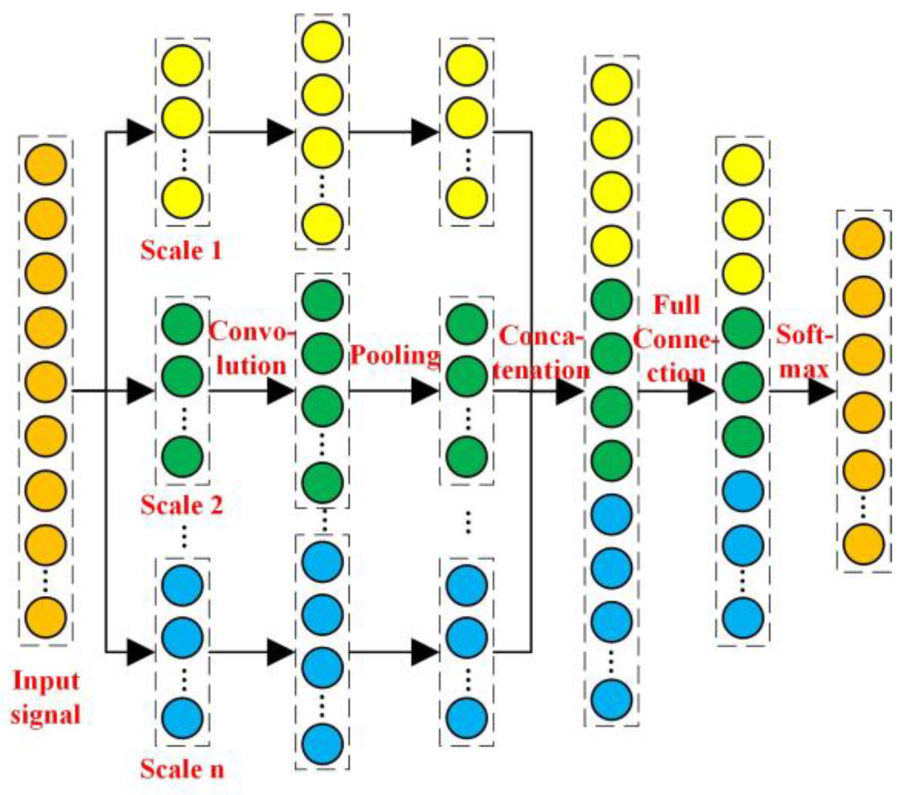
2.1. MSCNN
2.1.1. MSCL
2.1.2. Pooling Layer
2.1.3. Full Connection Layer and Softmax Classifier
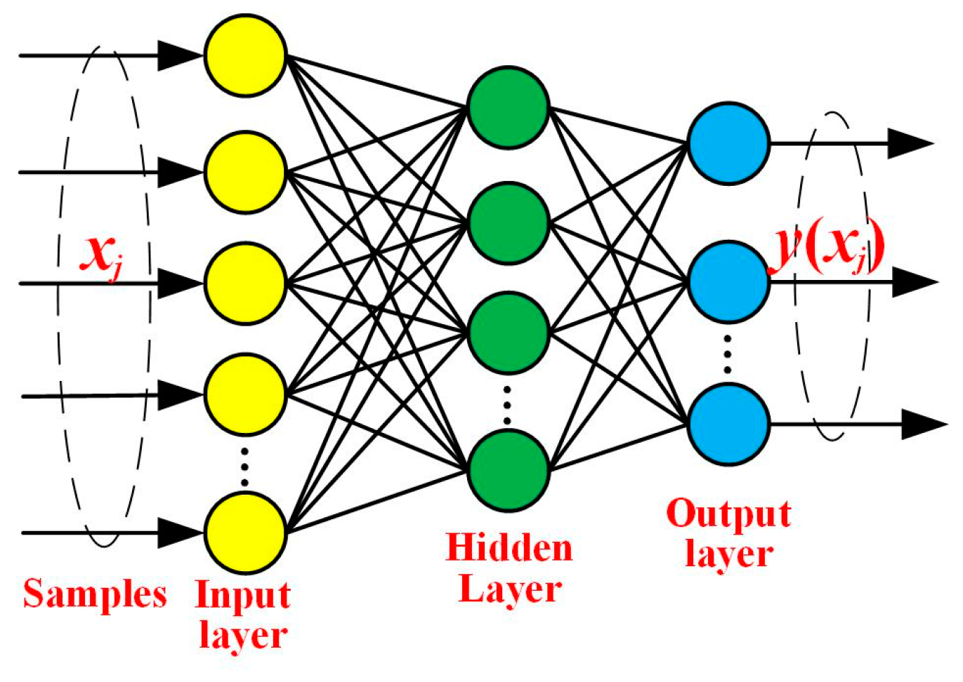
2.2. ELM
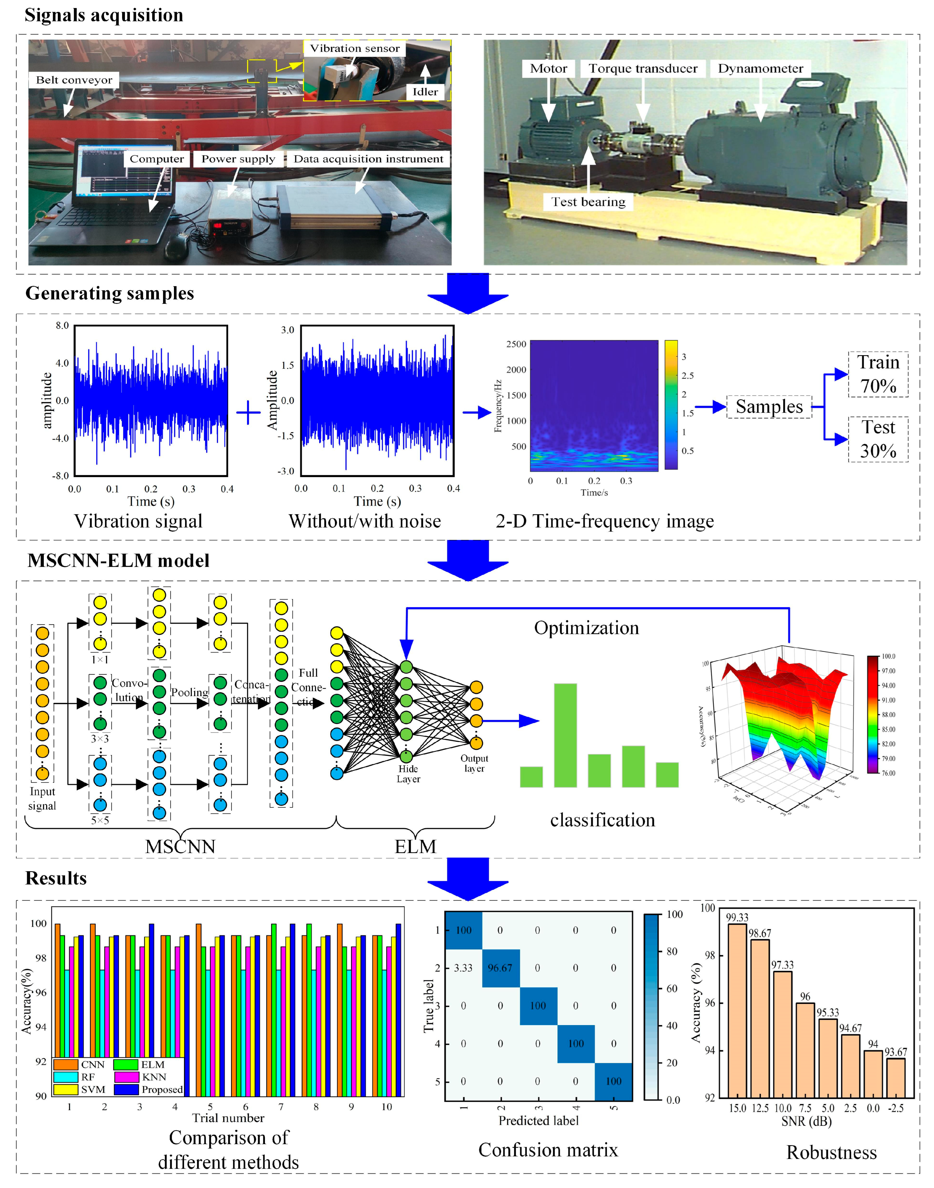
3. The Proposed Method
3.1. Design of the MSCNN-ELM
3.2. Fault Diagnosis Procedure Flow Chart Based on the MSCNN-ELM
4. Experimental Cases
4.1. Fault Diagnosis Based on the Self-Made Idler Dataset
4.1.1. Data Description
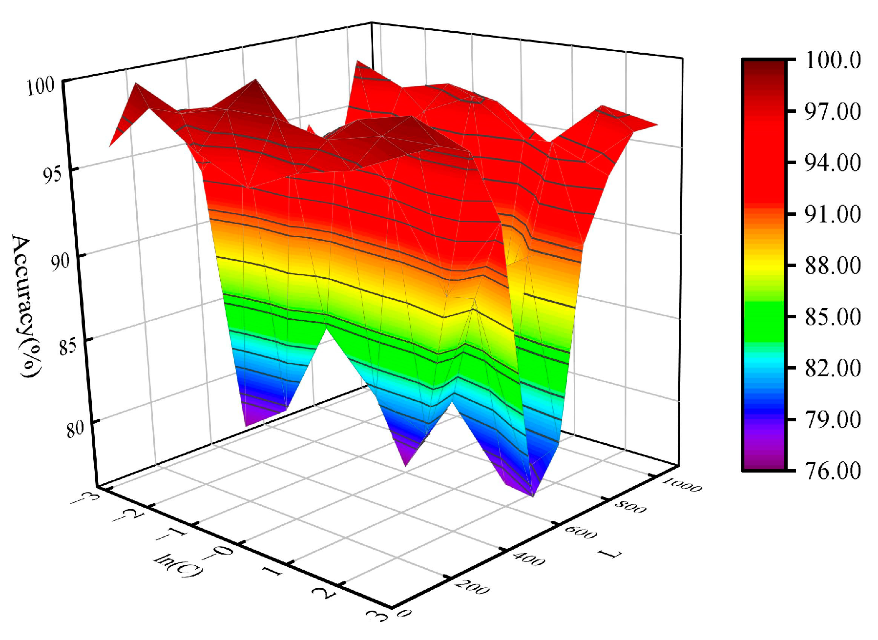
4.1.2. Parameter Optimization
4.1.3. The Efficiency of the MSCNN
4.1.4. Result Comparison with Other Methods
4.1.5. The Effect of Noise on the Model
4.2. Fault Diagnosis Based on the Bearing Dataset of the CWRU
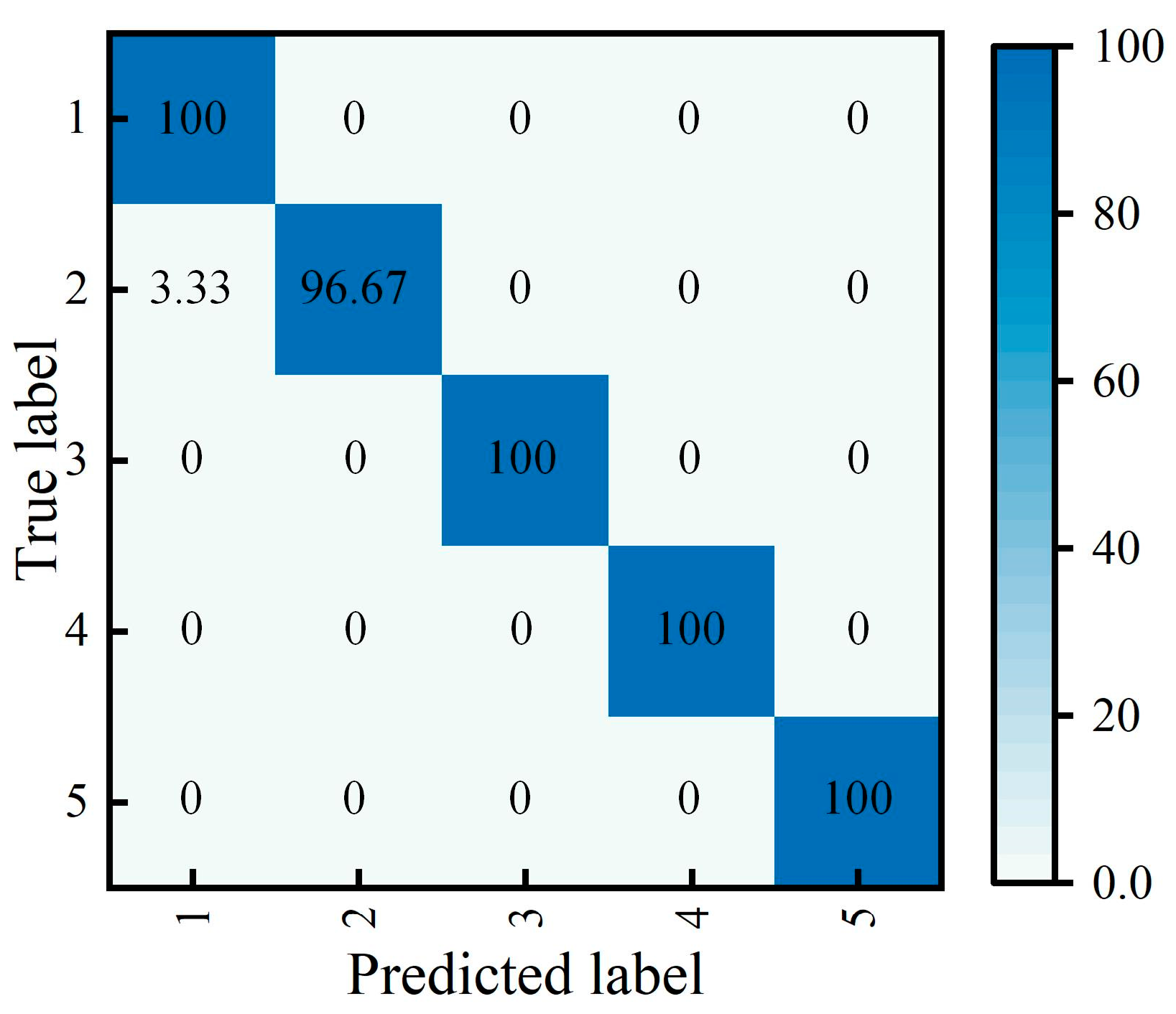
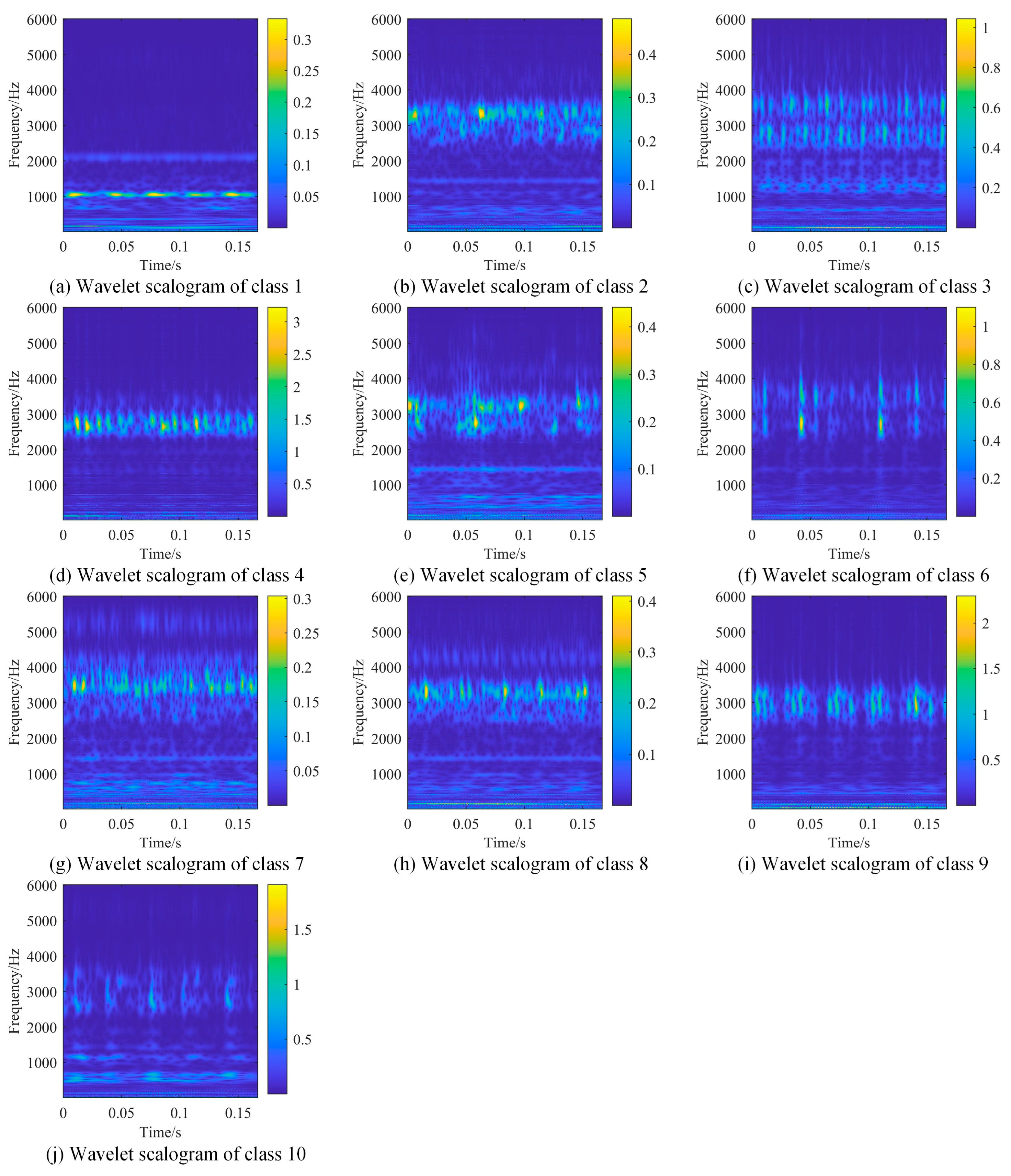
4.2.1. Data Description
4.2.2. The Efficiency of the MSCNN
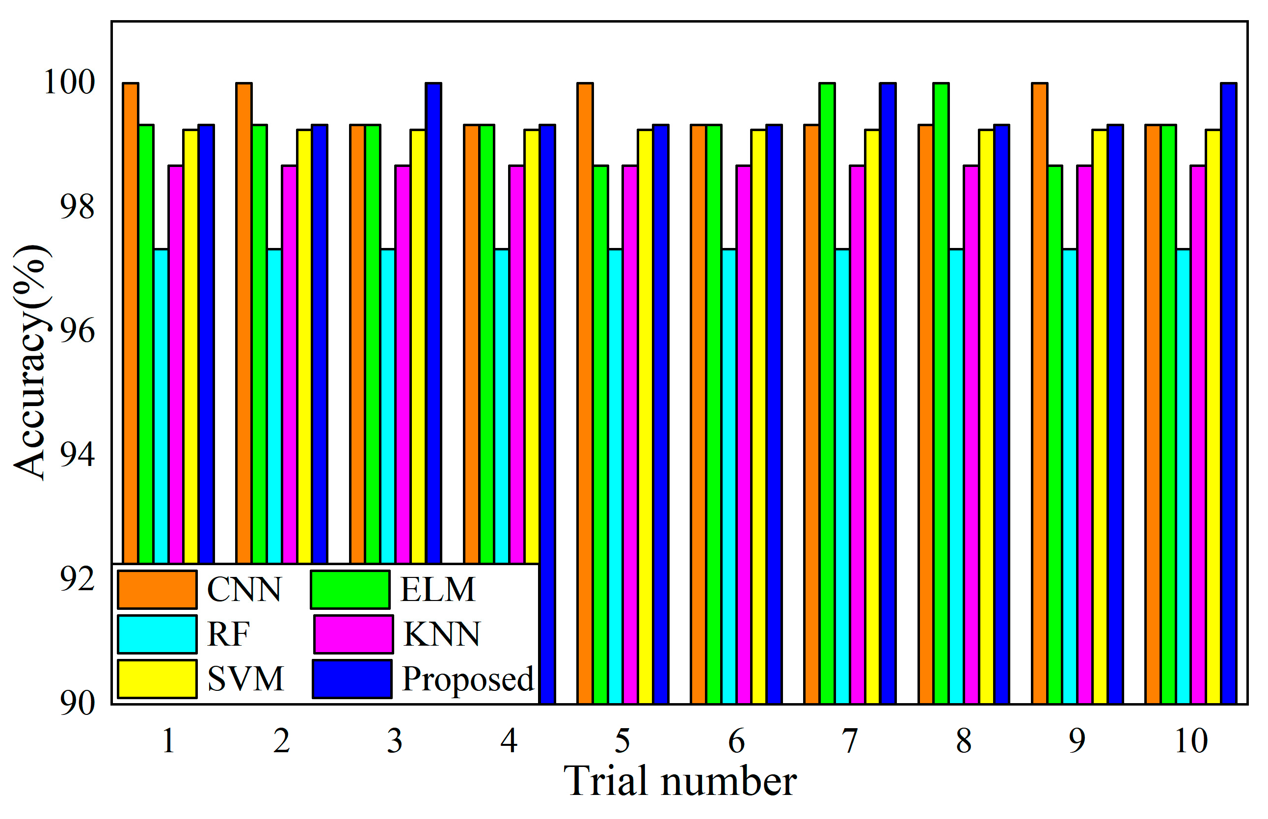
4.2.3. Results Comparison with Other Methods
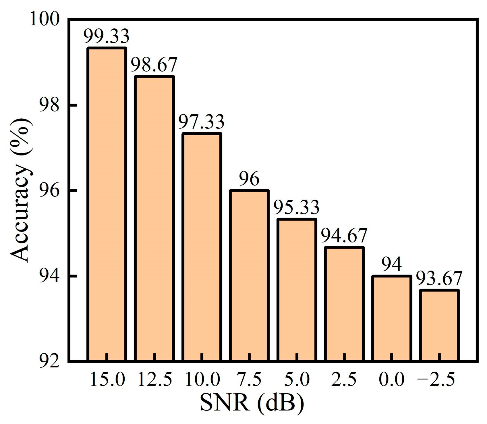
4.2.4. The Effect of Noise on the Model
5. Conclusions
Author Contributions
Funding
Institutional Review Board Statement
Informed Consent Statement
Data Availability Statement
Conflicts of Interest
References
- Zhao, B.; Zhang, X.; Li, H.; Yang, Z. Intelligent fault diagnosis of rolling bearings based on normalized CNN considering data imbalance and variable working conditions. Knowl.-Based Syst. 2020, 199, 105971. [Google Scholar] [CrossRef]
- Lei, Y.; Lin, J.; He, Z.; Zuo, M.J. A review on empirical mode decomposition in fault diagnosis of rotating machinery. Mech. Syst. Signal Process. 2013, 35, 108–126. [Google Scholar] [CrossRef]
- Cerrada, M.; Sánchez, R.-V.; Li, C.; Pacheco, F.; Cabrera, D.; Valente de Oliveira, J.; Vásquez, R.E. A review on data-driven fault severity assessment in rolling bearings. Mech. Syst. Signal Process. 2018, 99, 169–196. [Google Scholar] [CrossRef]
- Zhang, T.; Chen, J.; Li, F.; Zhang, K.; Lv, H.; He, S.; Xu, E. Intelligent fault diagnosis of machines with small & imbalanced data: A state-of-the-art review and possible extensions. ISA Trans. 2022, 119, 152–171. [Google Scholar] [PubMed]
- Xu, G.; Liu, M.; Jiang, Z.; Shen, W.; Huang, C. Online Fault Diagnosis Method Based on Transfer Convolutional Neural Networks. IEEE Trans. Instrum. Meas. 2020, 69, 509–520. [Google Scholar] [CrossRef]
- Wang, Z.; Yao, L.; Chen, G.; Ding, J. Modified multiscale weighted permutation entropy and optimized support vector machine method for rolling bearing fault diagnosis with complex signals. ISA Trans. 2021, 114, 470–484. [Google Scholar] [CrossRef]
- Vashishtha, G.; Chauhan, S.; Singh, M.; Kumar, R. Bearing defect identification by swarm decomposition considering permutation entropy measure and opposition-based slime mould algorithm. Measurement 2021, 178, 109389. [Google Scholar] [CrossRef]
- Tang, S.; Yuan, S.; Zhu, Y. Deep Learning-Based Intelligent Fault Diagnosis Methods toward Rotating Machinery. IEEE Access 2020, 8, 9335–9346. [Google Scholar] [CrossRef]
- Han, T.; Liu, C.; Wu, L.; Sarkar, S.; Jiang, D. An adaptive spatiotemporal feature learning approach for fault diagnosis in complex systems. Mech. Syst. Signal Process. 2019, 117, 170–187. [Google Scholar] [CrossRef]
- Onan, A. Bidirectional convolutional recurrent neural network architecture with group-wise enhancement mechanism for text sentiment classification. J. King Saud Univ.-Comput. Inf. Sci. 2022, 34, 2098–2117. [Google Scholar] [CrossRef]
- Wang, H.; Li, S.; Song, L.; Cui, L. A novel convolutional neural network based fault recognition method via image fusion of multi-vibration-signals. Comput. Ind. 2019, 105, 182–190. [Google Scholar] [CrossRef]
- Sun, Y.; Li, S. Bearing fault diagnosis based on optimal convolution neural network. Measurement 2022, 190, 110702. [Google Scholar] [CrossRef]
- Youcef Khodja, A.; Guersi, N.; Saadi, M.N.; Boutasseta, N. Rolling element bearing fault diagnosis for rotating machinery using vibration spectrum imaging and convolutional neural networks. Int. J. Adv. Manuf. Technol. 2019, 106, 1737–1751. [Google Scholar] [CrossRef]
- Cheng, Y.; Lin, M.; Wu, J.; Zhu, H.; Shao, X. Intelligent fault diagnosis of rotating machinery based on continuous wavelet transform-local binary convolutional neural network. Knowl.-Based Syst. 2021, 216, 106796. [Google Scholar] [CrossRef]
- Jiang, G.; He, H.; Yan, J.; Xie, P. Multiscale Convolutional Neural Networks for Fault Diagnosis of Wind Turbine Gearbox. IEEE Trans. Ind. Electron. 2019, 66, 3196–3207. [Google Scholar] [CrossRef]
- Deng, F.; Ding, H.; Yang, S.; Hao, R. An improved deep residual network with multiscale feature fusion for rotating machinery fault diagnosis. Meas. Sci. Technol. 2020, 32, 024002. [Google Scholar] [CrossRef]
- Huang, G.-B.; Bai, Z.; Kasun, L.L.C.; Vong, C.M. Local Receptive Fields Based Extreme Learning Machine. IEEE Comput. Intell. Mag. 2015, 10, 18–29. [Google Scholar] [CrossRef]
- Cox, D.; Pinto, N. Beyond simple features: A large-scale feature search approach to unconstrained face recognition. In Proceedings of the IEEE International Conference on Automatic Face and Gesture Recognition, Santa Barbara, CA, USA, 21–25 March 2011; pp. 8–15. [Google Scholar]
- Jarrett, K.; Kavukcuoglu, K.; Ranzato, M.; LeCun, Y. What Is the Best Multi-Stage Architecture for Object Recognition? In Proceedings of the IEEE 12th International Conference on Computer Vision (ICCV), Kyoto, Japan, 29 September–2 October 2009; pp. 2146–2153. [Google Scholar]
- Zhu, J.; Chen, N.; Peng, W. Estimation of Bearing Remaining Useful Life Based on Multiscale Convolutional Neural Network. IEEE Trans. Ind. Electron. 2019, 66, 3208–3216. [Google Scholar] [CrossRef]
- Jin, Y.; Qin, C.; Zhang, Z.; Tao, J.; Liu, C. A multi-scale convolutional neural network for bearing compound fault diagnosis under various noise conditions. Sci. China Technol. Sci. 2022, 65, 2551–2563. [Google Scholar] [CrossRef]
- Pang, Y.; Jia, L.; Zhang, X.; Liu, Z.; Li, D. Design and implementation of automatic fault diagnosis system for wind turbine. Comput. Electr. Eng. 2020, 87, 106754. [Google Scholar] [CrossRef]
- Wang, D.; Chen, Y.; Shen, C.; Zhong, J.; Peng, Z.; Li, C. Fully interpretable neural network for locating resonance frequency bands for machine condition monitoring. Mech. Syst. Signal Process. 2022, 168, 108673. [Google Scholar] [CrossRef]
- Chen, Z.; Gryllias, K.; Li, W. Mechanical fault diagnosis using Convolutional Neural Networks and Extreme Learning Machine. Mech. Syst. Signal Process. 2019, 133, 106272. [Google Scholar] [CrossRef]
- Li, X.; Yang, Y.; Hu, N.; Cheng, Z.; Cheng, J. Discriminative manifold random vector functional link neural network for rolling bearing fault diagnosis. Knowl.-Based Syst. 2021, 211, 106507. [Google Scholar] [CrossRef]
- Han, S.; Shao, H.; Cheng, J.; Yang, X.; Cai, B. Convformer-NSE: A Novel End-to-End Gearbox Fault Diagnosis Framework under Heavy Noise Using Joint Global and Local Information. IEEE/ASME Trans. Mechatron. 2022, 28, 340–349. [Google Scholar] [CrossRef]
- Zhong, H.; Lv, Y.; Yuan, R.; Yang, D. Bearing fault diagnosis using transfer learning and self-attention ensemble lightweight convolutional neural network. Neurocomputing 2022, 501, 765–777. [Google Scholar] [CrossRef]
- Wang, Y.; Ding, X.; Zeng, Q.; Wang, L.; Shao, Y. Intelligent Rolling Bearing Fault Diagnosis via Vision ConvNet. IEEE Sens. J. 2021, 21, 6600–6609. [Google Scholar] [CrossRef]
- Liu, Y.; Miao, C.; Li, X.; Ji, J.; Meng, D. Research on the fault analysis method of belt conveyor idlers based on sound and thermal infrared image features. Measurement 2021, 186, 110177. [Google Scholar] [CrossRef]
- Zhang, W.; Li, J.; Li, T.; Ge, S.; Wu, L. Research on feature extraction and separation of mechanical multiple faults based on adaptive variational mode decomposition and comprehensive impact coefficient. Meas. Sci. Technol. 2022, 34, 025110. [Google Scholar] [CrossRef]
- Wang, J.; He, Q.; Kong, F. Automatic fault diagnosis of rotating machines by time-scale manifold ridge analysis. Mech. Syst. Signal Process. 2013, 40, 237–256. [Google Scholar] [CrossRef]
- Wang, Z.; Zhang, Q.; Xiong, J.; Xiao, M.; Sun, G.; He, J. Fault Diagnosis of a Rolling Bearing Using Wavelet Packet Denoising and Random Forests. IEEE Sens. J. 2017, 17, 5581–5588. [Google Scholar] [CrossRef]
- Zhang, P.; Wen, G.; Dong, S.; Lin, H.; Huang, X.; Tian, X.; Chen, X. A Novel Multiscale Lightweight Fault Diagnosis Model Based on the Idea of Adversarial Learning. IEEE Trans. Instrum. Meas. 2021, 70, 3518415. [Google Scholar] [CrossRef]
- Liu, H.; Wang, Y.; Li, F.; Wang, X.; Liu, C.; Pecht, M.G. Perceptual Vibration Hashing by Sub-Band Coding: An Edge Computing Method for Condition Monitoring. IEEE Access 2019, 7, 129644–129658. [Google Scholar] [CrossRef]
- Liang, L.; Liu, F.; Li, M.; He, K.; Xu, G. Feature selection for machine fault diagnosis using clustering of non-negation matrix factorization. Measurement 2016, 94, 295–305. [Google Scholar] [CrossRef]


| Bearing Conditions | Number of Samples | Class Label |
|---|---|---|
| Health | 200 | 1 |
| IF | 200 | 2 |
| OF | 200 | 3 |
| IR | 200 | 4 |
| NR | 200 | 5 |
| Model | Training Accuracy (%) | Testing Accuracy (%) | Training Time (s) | Testing Time (s) |
|---|---|---|---|---|
| CNN-ELM | 100 ± 0 | 99.40 ± 0.60 | 1.15 | 0.08 |
| MSCNN-ELM | 100 ± 0 | 99.53 ± 0.47 | 1.12 | 0.08 |
| Model | Training Accuracy (%) | Testing Accuracy (%) | Training Time (s) | Testing Time (s) |
|---|---|---|---|---|
| CNN | 100 ± 0 | 99.60 ± 0.40 | 3.25 | 0.23 |
| ELM | 100 ± 0 | 99.32 ± 0.68 | 1.02 | 0.07 |
| RF | 100 ± 0 | 97.33 ± 0 | 1.13 | 0.08 |
| KNN | 100 ± 0 | 98.67 ± 0 | 1.10 | 0.08 |
| SVM | 100 ± 0 | 99.25 ± 0 | 1.08 | 0.11 |
| MSCNN-ELM | 100 ± 0 | 99.53 ± 0.47 | 1.12 | 0.08 |
| Load (hp) | Bearing Conditions | Fault Diameters (inch) | Number of Samples | Class Label |
|---|---|---|---|---|
| 0, 1, 2, and 3 | Health | 0 | 400 | 1 |
| BF | 0.007 | 400 | 2 | |
| IF | 0.007 | 400 | 3 | |
| OF | 0.007 | 400 | 4 | |
| BF | 0.014 | 400 | 5 | |
| IF | 0.014 | 400 | 6 | |
| OF | 0.014 | 400 | 7 | |
| BF | 0.021 | 400 | 8 | |
| IF | 0.021 | 400 | 9 | |
| OF | 0.021 | 400 | 10 |
| Model | Training Accuracy (%) | Testing Accuracy (%) | Training Time (s) | Testing Time (s) |
|---|---|---|---|---|
| CNN-ELM | 99.85 ± 0.11 | 99.37 ± 0.21 | 9.37 | 0.67 |
| MSCNN-ELM | 99.88 ± 0.13 | 99.43 ± 0.15 | 9.45 | 0.68 |
| Model | Training Accuracy (%) | Testing Accuracy (%) | Training Time (s) | Testing Time (s) |
|---|---|---|---|---|
| CNN | 99.80 ± 0.13 | 99.47 ± 0.20 | 28.55 | 2.04 |
| ELM | 99.99 ± 0.01 | 99.33 ± 0.22 | 8.97 | 0.64 |
| RF | 100 ± 0 | 98.75 ± 0 | 9.98 | 0.71 |
| KNN | 99.82 ± 0 | 99.33 ± 0 | 9.16 | 0.65 |
| SVM | 100 ± 0 | 99.31 ± 0 | 10.08 | 0.72 |
| MSCNN-ELM | 99.88 ± 0.13 | 99.43 ± 0.15 | 9.45 | 0.67 |
Disclaimer/Publisher’s Note: The statements, opinions and data contained in all publications are solely those of the individual author(s) and contributor(s) and not of MDPI and/or the editor(s). MDPI and/or the editor(s) disclaim responsibility for any injury to people or property resulting from any ideas, methods, instructions or products referred to in the content. |
© 2023 by the authors. Licensee MDPI, Basel, Switzerland. This article is an open access article distributed under the terms and conditions of the Creative Commons Attribution (CC BY) license (https://creativecommons.org/licenses/by/4.0/).
Share and Cite
Zhang, W.; Li, J.; Huang, S.; Wu, Q.; Liu, S.; Li, B. Application of Multi-Scale Convolutional Neural Networks and Extreme Learning Machines in Mechanical Fault Diagnosis. Machines 2023, 11, 515. https://doi.org/10.3390/machines11050515
Zhang W, Li J, Huang S, Wu Q, Liu S, Li B. Application of Multi-Scale Convolutional Neural Networks and Extreme Learning Machines in Mechanical Fault Diagnosis. Machines. 2023; 11(5):515. https://doi.org/10.3390/machines11050515
Chicago/Turabian StyleZhang, Wei, Junxia Li, Shuai Huang, Qihang Wu, Shaowei Liu, and Bin Li. 2023. "Application of Multi-Scale Convolutional Neural Networks and Extreme Learning Machines in Mechanical Fault Diagnosis" Machines 11, no. 5: 515. https://doi.org/10.3390/machines11050515
APA StyleZhang, W., Li, J., Huang, S., Wu, Q., Liu, S., & Li, B. (2023). Application of Multi-Scale Convolutional Neural Networks and Extreme Learning Machines in Mechanical Fault Diagnosis. Machines, 11(5), 515. https://doi.org/10.3390/machines11050515