Abstract
This paper proposes a new pneumatic modular joint to address the problem of balancing compliance and load-bearing capacity for soft robots. The joint possesses characteristics that allow for omnidirectional deformation and dynamically adjustable stiffness. In this study, mathematical models were established to describe the deformation and stiffness variability of the joint. Corresponding relationships between gas pressure and deformation and magnetic field strength and module stiffness were derived through numerical analysis. Finite element simulations were conducted to investigate the changes in pressure and deformation under different stiffness conditions and the changes in magnetic field strength and joint stiffness under various deformation states. Finally, experimental validation was performed to verify the theoretical calculations and simulation results, demonstrating excellent coupling characteristics between stiffness and compliance for the proposed joint.
1. Introduction
A soft robot has good flexibility [1], more freedom, adapts to active and passive deformation, and is friendly to dynamic, unknown, and unstructured environments; it is also widely used in military reconnaissance, disaster rescue, and scientific exploration, and other vital fields. However, due to the low stiffness of compliant structures and soft materials [2], the bearing capacity of soft robots could be much higher. More carrying capacity [3] has become the most significant obstacle limiting the application range of soft robots, and it is also a common critical technical problem facing this field [4].
In the current research in this area, various soft robots have been introduced [5]. Natural creatures inspire most of soft robots. The driving methods of the soft robot include pneumatic [6], electroactive polymers (EAPs) [7], shape memory alloy [8], magnetorheological fluid [9], and cable-driven methods [10]. Actuators with a network of chambers and uniformly distributed channels of the PNEU-NET software drive [11] have the advantages of large deformation and high efficiency. It has been widely innovated and applied by researchers. There are several methods for varying stiffness with different techniques, such as variable stiffness materials [12], electrically induced dangerous stiffness materials [13], and pressure-induced unstable stiffness methods [14]. Luojing Huang et al. [15] proposed a variable stiffness pneumatic soft robot based on a magnetorheological lubricant, which can grip and adapt to various object surfaces with high flexibility and accuracy. Revanth Konda et al. [16] proposed a design for using a twisted string actuator to drive the gripper of soft robots. Experimental results demonstrated that this delicate claw has good gripping performance and high load output. Ali Shiva et al. [17] took inspiration from the aggressive behavior of octopus arms and proposed a variable stiffness method that can control the attitude and stiffness of the robot simultaneously by pneumatic and tendon-driven reverse operations. George B. Crowley et al. [18] developed a soft robot gripper with variable stiffness using a novel positive pressure layer jamming technique to adjust the fixture stiffness and manufacturing the fixture in two materials through additive manufacturing. Experimental tests showed that the gripper could change its stiffness about 25 times under positive layer jamming interference and has a higher payload capacity. Yanzhi Zhao et al. [19] proposed an extensive range of variable stiffness self-locking soft continuous robots based on the interference phenomenon. The textile smooth rope restraint mechanism based on the particle interference mechanism uses the low elasticity and high toughness of fiber, the excellent fluidity of spherical particles, and the rigidity of particles themselves. A variable stiffness self-locking soft robot is constructed. The shape of the robot will not change significantly after the stiffness change. Al Abeach, L et al. [20] developed a variable stiffness multi-finger dexterous gripper. The gripper uses pneumatic muscles for compliance, and increasing the pressure on all actuators can improve grip stiffness independently without changing the position of the fingers. However, the deformation recovery could be better. Loai Al Abeach et al. [21] proposed designing, analyzing, and testing a variable stiffness three-finger soft gripper. It uses pneumatic muscles to drive the finger and changes the stiffness of the finger by particle clamping. As the stiffness of the finger increases due to friction caused by the granular interference, the positioning accuracy of the extended finger (i.e., opening the grip) decreases; that is, the muscle is not pulled back to the original extended length. Yujia Li et al. [22] proposed a flexible robot with variable stiffness based on pre-inflation, particle interference, and origami technology. When the origami structure is compressed, the particles are squeezed by the compression force and the increased pressure of the three air chambers, increasing the robot’s overall stiffness. Tao Wang et al. [23] proposed a new layer interference variable stiffness technology, which uses electrostatic attraction to squeeze the material layer to generate friction, which creates interference. It is characterized by high stiffness variation and space saving. However, the formation of local low-pressure areas between the contact surfaces results in a degree of randomness in the stiffness generated under applied voltage. Liu Zhaoyu et al. [24] proposed a method combining soft crawling robots with variable stiffness technology to achieve the obstacle avoidance movement of soft crawling robots. When a modular biomimetic soft robot with variable stiffness adjustment passes through obstacles of the same height, there will be no apparent collision with obstacles. Although there are many research results on variable stiffness, the coupling characteristics of deformation and variable stiffness need be studied more deeply [25,26]. However, considering soft robots’ flexibility and bearing capacity simultaneously requires good rigid-flexible coupling characteristics [27,28]. From the research literature, there are few reports on this aspect.
Therefore, this study focuses on the innovative new modular soft robot joint with variable stiffness and researches the coupling characteristics of joint deformation and variable stiffness. We have established and solved a variable stiffness model for modular smooth joints, which includes deformation and correlates with gas pressure and joint stiffness with an applied current. The finite element analysis method is used to simulate and analyze the deformation characteristics and variable stiffness characteristics of modular joints based on the Yeoh model, and the rigid-flexible coupling characteristics of modular joints are revealed through deformation and variable stiffness tests.
2. Structure Principle
The new variable stiffness modular soft robot joint body material is made of 50 A silicone rubber. The performance of silicone rubber 50 A is shown in Table 1; the whole modular joint consists of four driving modules. As shown in Figure 1, each driver module is divided into three parts: It is composed of a variable stiffness system, a flexible deformation system, and a connecting end cover. As shown in the upper left view and upper right view of Figure 1, the axis of the flexible joint is the first channel for installing polyurethane foam pads, the outer circumference of the flexible joint is provided with a second channel for installing wires, and between the first channel and the second channel there are four embedded pneumatic network channels at 90° to each other, distributed in the entire structure of the joint, and, through the combination of positive and negative pressure gas changes of different pressures of the four channels, different degrees of bending in all directions can be realized.

Table 1.
Performance of silicone rubber 50 A.
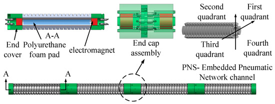
Figure 1.
Modular joint.
The variable stiffness system consists of electromagnets at both ends of the joint and polyurethane foam pads filled with magnetorheological fluid, which are centrally placed at the pivot position of each joint. The DC power supply powers the electromagnet. The current in the electromagnet circuit is adjusted by changing the resistance of the varistor in the electromagnet loop, so that the electromagnet produces different magnetic field strengths. The magnetic field strength’s [29] size changes the viscosity of the magnetorheological fluid to realize the dynamic and continuous adjustment of modular joint stiffness.
The flexible deformation system includes a pneumatic flexible pneumatic joint, which can bend and deform with the change of air pressure, and a pneumatic system that provides an air source for the joint. Each air chamber of the common is connected at the bottom. Each drive module has four air pipes, which are inserted into the pneumatic channel connecting the end cover. When inflating, the air passes through the inflatable tube to each chamber of the soft joint. Each compartment expands as the chamber pressure increases, causing the smooth joints to bend [30]. Figure 2b shows the air chamber after expansion.
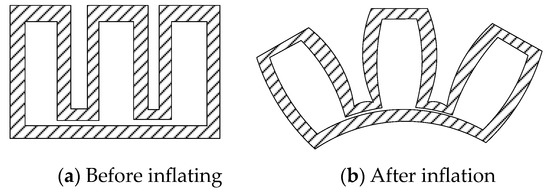
Figure 2.
Section of air chamber.
The end caps of the two ends of the flexible joints are 3D printed with PLA material and placed on polyurethane foam pads filled with magnetorheological fluid. Embedded pneumatic network channels in two adjacent loose joints are connected through quick joints and hoses in the end covers.
3. Modeling and Solving
Deformation and variable stiffness are two important indexes to evaluate modular joints. The modular joint is modeled mathematically from these two aspects.
3.1. Deformation Modeling
As shown in Figure 2a, the cavity in the exhausted state is rectangular, and the elongation of a single embedded pneumatic network channel of the joint after inflation and expansion is less than the elongation away from the axis layer so that the joint is convex and bent away from the axis layer.
To simplify the model, the following assumptions are proposed: (1) the material used cannot be compressed; and (2) the soft joint keeps constant curvature bending during bending. The parameters of the air chamber [31] are shown in Figure 3a, and their values are shown in Table 2.
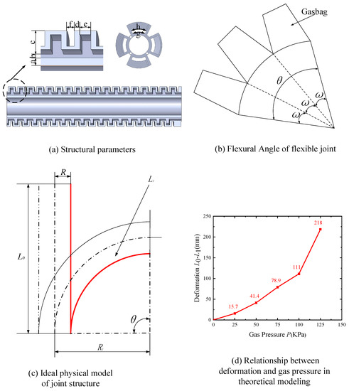
Figure 3.
Articular structure.
Table 2.
Structural parameters of the air cavity.
During joint design, each air cavity is designed with a symmetric structure, and the structural parameters are consistent, as shown in Figure 3a. Therefore, when ventilating an embedded pneumatic network channel, in the medium is subjected to the same pressure and bending angle.
As shown in Figure 3b, the total number of air cavities in this channel is , where the bending angle of each air cavity is , then the whole bending angle is:
The relationship between gas pressure and bending angle can be solved by the structural parameters of a single air cavity, assuming that the neutral axis length is unchanged when the modular joint is deformed. The bending deformation changes uniformly in the length direction to establish an ideal physical model of the joint structure. As shown in Figure 3c, the relationship between gas pressure and bending angle can be converted into the relationship between gas pressure and deformation.
Under the condition of ignoring the self-weight of the joint and its external force, it can be seen from the law of conservation of energy that the work performed by the pneumatic system to inflate the embedded pneumatic network channel is completely converted into the power of silica gel deformation, that is, the work performed by the gas pressure is equal to the energy of the deformation of the soft joint, which is expressed by its formula as:
Among them, is the gas pressure of the pneumatic system to inflate the embedded pneumatic network channel, is the volume of the air cavity after inflation, is the volume of the silica gel after inflation, and is the strain energy. Since it is assumed that the silica gel is incompressible before and after inflation, its volume remains the same, so it can be obtained:
is the total volume after inflation, so , thus:
where is the primary elongation in the direction of the air cavity length, , and is the curvature radius of joint bending. Taking the derivative of and combining Equations (3) and (4), the relationship between the bending angle of a single air cavity and the gas pressure can be obtained:
where , silica gel material is a second-order Yeoh model, so , and, among them, . When the gas pressure is set to 0 kPa, 25 kPa, 50 kPa, 75 kPa, 100 kPa, and 125 kPa, respectively, the bending angle results of corresponding joints are solved, as shown in Table 3.
Table 3.
Bending angles of joints under different pressures.
As shown in Figure 3c, when the gas with a certain pressure is injected into the joint, the relationship between the deformation and bending angle is as follows:
where is the distance of the edge of the joint from the neutral axis, is the initial length of the joint, is the length after joint deformation, is the bending angle of the joint, and is the bending radius of the joint.
The bending angle in Table 3 above is converted into the deformation amount by Formula (7), and the deformation amount is used to reflect the deformation effect of the modular joint. The relationship between the deformation amount and gas pressure in the theoretical model is shown in Figure 3d.
The image of the relationship between gas pressure and joint deformation obtained by kinematically modeling the modular joint conceptual model is shown in Figure 3d. When the gas pressure changes from 0 to 100 kPa, the deformation increases approximately linearly with the increase of gas pressure. The gas pressure increases slightly after 100 kPa, the deformation has a large increase, and the maximum pressure of the drive module does not exceed 125 kPa [32] after strength verification, and therefore the expected deformation effect can be achieved.
3.2. Variable Stiffness Modeling
After the soft joint is deformed, a certain stiffness is required to enhance the bearing capacity, and the greater the stiffness is, the stronger is the bearing capacity. The robot’s stiffness includes various rigidities, such as static stiffness, dynamic stiffness, servo stiffness, and mechanical stiffness. Considering that the bending deformation process of soft actuators has little influence on dynamic stiffness, this paper only analyzes the change of static stiffness [33]. Electromagnetic field’s magnetic induction intensity reflects magnetorheological fluid’s variable stiffness. The following series of derivations shows that the stiffness characteristics of the variable stiffness system model can be obtained by introducing different currents.
The transformation of force and motion is introduced to establish a variable stiffness model of modular joints. Under the action of external force , the rotational momentum of the joint is . When the external energy and the rotational speed of the common are small enough, they can be regarded as an approximately linear relationship:
where represents the stiffness of the joint.
For the static stiffness of the drive module, the modular joint can be regarded as a system. When the joint is stationary, the velocity and angular velocity are zero. Therefore, the angular velocity, is equal to zero, and the angular acceleration, , is equal to zero. Therefore the torque, , acting on the joint satisfies:
Among them, is the static stiffness of the modular joints.
The operating mode of the variable stiffness model in the drive module is shown in Figure 4a. When the electromagnet is not energized, magnetorheological fluid is not magnetic. Currently, magnetorheological fluid is liquid, with low viscosity and almost no damping moment. The effect of variable stiffness in flexible joints is virtually zero. When the electromagnet is energized, magnetorheological fluid particles generate magnetism and connect into a chain structure, and magnetorheological fluid can become a semi-solid state with high viscosity within milliseconds [34]. When the magnetic field encountered by the magnetorheological fluid increases, the magnetorheological fluid becomes a solid-like form. In this change, the shear stress of the magnetorheological fluid gradually increases, resulting in damping torque. The damping torque diagram of the structure is shown in Figure 4b.
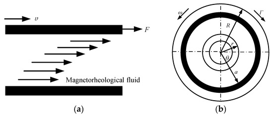
Figure 4.
Change under a magnetic field of magnetorheological liquid. (a) Schematic diagram of magnetorheological fluid flow without magnetic field; (b) damping torque of strong magnetic field.
To solve the flow of the magnetorheological fluid in the driving module, the following assumptions are made [35]:
- (1)
- The magnetorheological fluid cannot be compressed in the flow process and can maintain long-term stability;
- (2)
- The flow effect of magnetorheological fluid in both axial and radial directions of the joint is negligible;
- (3)
- The flow velocity of the magnetorheological fluid in modular joints is only related to the joint radius;
- (4)
- The magnetorheological fluid has the same pressure in the radial direction of the joint.
The distribution of the damping torque is concentric circles with a small radius, , and a large radius, . When the modular joint moves with angular velocity , the joint will produce a torque, , in the direction opposite to the angular velocity. Let the annular area of the disk be and the damping torque produced by the disk be .
where is the magneto-induced torque generated by the action of the applied magnetic field on the viscosity of the magnetorheological fluid, and is the non-magneto-induced torque generated by the density of the magnetorheological fluid after yield.
From the above formula, it can be seen that the stiffness change of the drive module is related to the change in magnetorheological fluid viscosity. When the electromagnet is not energized, the magnetorheological fluid is not magnetic, and the magnetorheological fluid at this time is a liquid form with low viscosity, and the constitutive relationship at any point is:
where is the shear stress generated by the magnetorheological fluid in modular joints, is the viscosity of the magnetorheological fluid in the absence of a magnetic field, and is the shear strain caused by the magnetorheological fluid viscosity in modular joints.
where is the shear yield stress generated by the magnetorheological fluid in the modular joint. The magnitude of the magnetic field generated by the electromagnet is positively correlated with the shear yield stress caused by the magnetorheological fluid.
Therefore, electromagnetic field magnetic induction strength analysis can reflect the variable stiffness characteristics of magnetorheological fluids. The magnetization curve of magnetorheological fluid is shown in Figure 5.
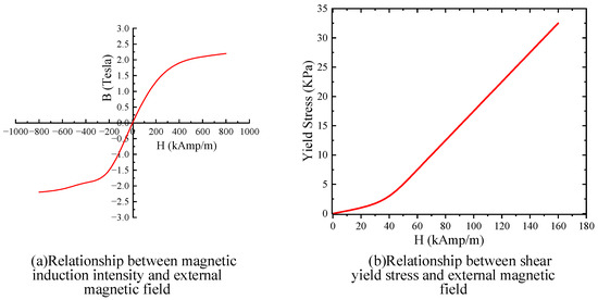
Figure 5.
Magnetization properties of magnetorheological fluids.
The stiffness change of the driving module is related to the viscosity change of the magnetorheological fluid. It can be seen from Figure 5 that the magnetic induction intensity, , increases linearly with the increase of the magnetic field intensity within 400 kAmp/m, so the magneto-induced yield stress, , and the external magnetic field intensity, H, have an approximately linear relationship:
The permeability, , of fluid is:
Through Equations (10) and (11), we can obtain:
Magnetic field strength calculation formula:
Substituting Equation (13) into Equation (10), we can obtain:
Equation (17) shows the relationship between magneto-induced shear yield stress, electromagnet parameters, and applied current.
4. Simulation Analysis
The finite element method is used to establish a model, simulate and analyze the aerodynamic loading process of the pneumatic soft robot, and investigate the deformation effect of the flexible joint by introducing different gas pressures into the channel under the same magnetic induction strength. The shear modulus of the joint investigates the variable stiffness effect under different magnetic induction strengths.
The finite element software used for simulation is ANSYS workbench. Boundary conditions for simulation are as follows. Two bodies are imported into workbench mechanical: one is a pneumatic software channel, and the other is a magnetic flow layer with shear modulus, density, and mass set. The two bodies are set as the same part, that is, the grid common nodes of the two bodies are realized. Set one end of the joint as a fixed support end and the other as a free end, and apply a pressure load on the inner wall channel.
Simulated mesh size: set the mesh size to 2 mm.
Simulated grid cells: these are set to automatic for intelligent partitioning.
The steps are:
- Pneumatic soft channel and magnetic fluid structure are set up. The material density of the pneumatic soft channel is 1200 kg/m3. The Yeoh elastomer model is adopted, C10 = 0.11, and C20 = 0.02. Create a new MDL material and set the shear modulus as shown in G in Figure 6. Poisson’s ratio is 0.45, and density is 3450 kg/m3.
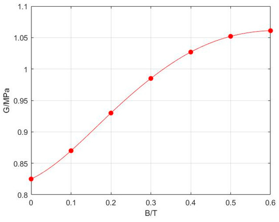 Figure 6. Shear modulus of magnetic fluid under different magnetic induction intensities.
 - Import the model and divide the grid. Set the mesh shape to tetrahedron and the cell size to 2 mm.
- Apply load and constraint: set the right end plane of the soft joint as fixed support and the left end as free end. The load form is pressure, and the acting surface is the wall of the pneumatic channel.
- Open the large deformation mode (for the simulation of elastomer with large deformation), and set the maximum number of iteration sub-steps to 10,000.
- Start simulation calculation to obtain strain and stress data and cloud image
4.1. Parameter Settings
The viscosity parameter at a certain magnetic induction strength is converted into the material’s shear modulus, replacing the magnetorheological fluid’s properties to determine the influence on the system deformation under different working conditions through simulation.
A disc-type electromagnet is selected, and its structural parameters are shown in Table 4.
Table 4.
Structure parameters of the electromagnet.
4.2. Deformation Simulation
4.2.1. Deformation Simulation without Magnetic Field
The constitutive model is established through the Yeoh model, and its density function is expressed as binomial parameters in the form of:
where , is the axial stretch ratio, is the radial stretch ratio, is the circumferential primary stretch ratio, and and are the constant coefficients of the Yeoh model silica gel materials. Make the material constant coefficients , and .
The theoretical model of a single soft joint is taken as the object, and the bending deformation angle is observed by applying 0–125 kPa gas pressure to a single channel of the flexible actuator, as shown in Figure 7.
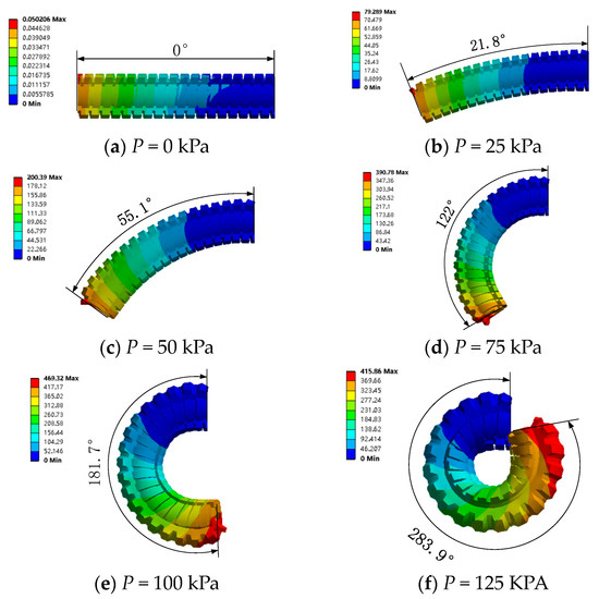
Figure 7.
Strain maps of joints at different pressures.
It can be seen from Figure 7 that the bending angle of the soft body joint gradually increases with the increase of gas pressure, the stress concentration appears on the side close to the gas source, and the stress gradually decreases on the side away from the air source. With the increase of deformation, the stress concentration area begins to expand inward. The relationship curve between gas pressure and joint deformation is shown in Figure 8.
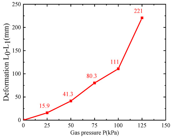
Figure 8.
Variation of deformation with gas pressure.
It can be seen from Figure 8 that, when the gas pressure changes from 0 to 111 kPa, the deformation is roughly linearly related with the increase of gas pressure, and the deformation is significantly deformed with the increase of gas pressure after 111 kPa, which is prone to excessive material stress concentration and the risk of material rupture caused by over-deformation.
4.2.2. Pressurize Single Channel with Different Magnetic Fields
The coupling of the soft gas channel and magnetorheological fluid is simulated by the fluid-solid bidirectional coupling method, which requires much calculation and has low simulation efficiency.
After analyzing the properties of the Mr fluid layer, it is found that the properties of the magnetic fluid are closer to those of the solid when the viscosity of the magnetic fluid is more significant, so the magnetic fluid properties are considered to be transformed into the viscoelasticity of the stable. In the bending deformation of the pneumatic channel, the internal magnetic fluid is mainly subjected to the shear load imposed by the inner wall of the track. When the stiffness of the magnetic fluid is more muscular, the response to the shear load is more robust, and the shear modulus of the solid is larger. Therefore, according to the positive correlation between the shear modulus of the magnetic fluid and its viscosity, the material of the magnetorheological liquid layer is set as a solid with a different shear modulus. In statics, the shear modulus of solid material is used to simulate the viscosity of the magnetic fluid, and the simulation of deformation under different viscosities of magnetic fluid is completed. The contact form between the magnetorheological liquid layer and the software channel:friction constraint is adopted; that is, normal separation and tangential slip are allowed. The validity of the model was also confirmed in the subsequent experimental phase.
Table 5 shows other gradient gas pressures for a single track.
Table 5.
Parameter setting of simulation conditions for pressurizing single channel.
As shown in Figure 9, when the viscosity is 55 Pa·s and the gas pressure is 25 kPa, 50 kPa, 75 kPa, 100 kPa, and 125 kPa, respectively, the deformation amount of soft joint gradually increases with the increase of air pressure.

Figure 9.
Deformation of a single channel with different gas pressures (τ = 15 Pa·s).
When a single channel is introduced to a gas pressure of 75 kPa, there are bending and stress changes, as shown in Figure 10, and the viscosity increases gradually as the magnetic field increases. By comparing the bending degree of soft joints with viscosities of 0.15 Pa·s, 15 Pa·s, 38 Pa·s, 55 Pa·s, and 72 Pa·s, it can be seen that the greater the viscosity is, the less obvious is the joint deformation, the less obvious is the surface stress, and the greater is the shear force.
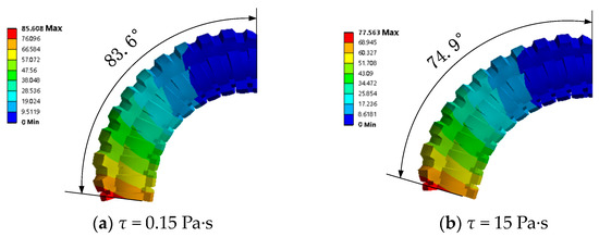
Figure 10.
Deformation simulation of different viscosities (P = 75 kPa).
Similarly, since the working conditions of channel 1, channel 2, channel 3, and channel 4 are the same, the analysis results of gas pressure entering other media can be obtained by the same analysis method.
4.2.3. Pressurize the Two Channels under Various Magnetic Fields
To study the influence of variable stiffness on omnidirectional deformation, conditions of 1–5 were applied to adjacent channels one and 2, as shown in Table 6. The two adjacent channels with viscosity 55 Pa·s simultaneously pass the gas pressures of 15 kPa, 30 kPa, 45 kPa, 60 kPa and 75 kPa, and the bending angle and stress simulation diagrams of the soft joint are shown in Figure 11.
Table 6.
Simulation condition parameter setting for double channel pressurization.
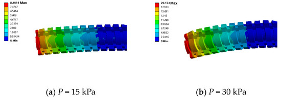
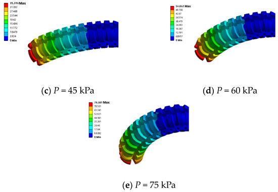
Figure 11.
Deformation simulation of two adjacent channels with different gas pressures (τ = 55 Pa·s).
When the gas pressure of 75 kPa is introduced into the adjacent two channels, there are bending and stress changes, as shown in Figure 12, and the viscosity increases gradually as the magnetic field increases. By comparing the bending degree of soft joints with viscosities of 0.15 Pa·s, 15 Pa·s, 38 Pa·s, 55 Pa·s, and 72 Pa·s, it can be seen that the greater the viscosity is, the less obvious is the joint deformation, the less obvious is the surface stress, and the greater is the shear force.
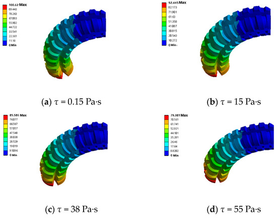
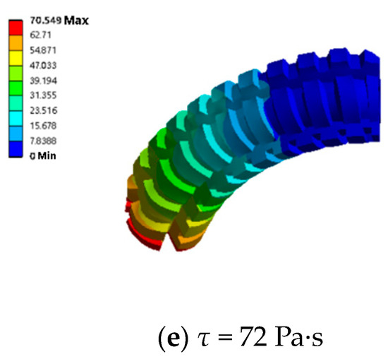
Figure 12.
Corresponding deformation of two adjacent channels at different viscosities (P = 75 kPa).
4.3. Variable Stiffness Simulation
In this section, the variable stiffness model is established for stiffness simulation analysis, and the stiffness analysis method is determined in Section 3.2. In measuring the variable stiffness characteristics, the magnetic induction strength of the electromagnetic field is used to reflect the variable stiffness characteristics of the magnetorheological fluid.
When the driving module is fed with 75 kPa air pressure, the variable stiffness system is under the applied currents of 0.1 A, 0.2 A, 0.3 A, 0.4 A, and 0.5 A, respectively. As shown in Figure 13, with the increase of the external magnetic field strength, the stiffness of the drive module increases, and the deformation decreases.
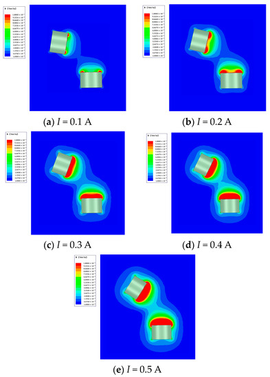
Figure 13.
Distribution of magnetic field under different currents at 75 kPa.
Under the magnetic field of a 0.4 A applied current, when the pressures of the drive module are 0 kPa, 25 kPa, 50 kPa, 75 kPa, 100 kPa, and 125 kPa, as shown in Figure 14, with the increase of deformation, the magnetic field at the center of the two electromagnets changes from strong to weak and then to vigorous.
Figure 14.
Magnetic field distribution with different gas pressures at 0.4A current.
5. Test
5.1. Experimental Design
To verify the correctness of the theoretical and simulation results, a test platform for the analysis of rigid and flexible characteristics of modular soft joints was built. As shown in Figure 15, two brake clamps constrain the inflatable end and the magnetorheological liquid end, so that the whole structure is in a horizontal state. The bending sensor, a flex sensor 4.5, is attached to the axial direction of the joint to measure the bending angle. When the flex sensor 4.5 is bent, its resistance value changes. The bending state is detected by measuring its resistance. Thus, by changing the magnetic field strength of the electromagnet, its stiffness is variable.
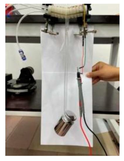
Figure 15.
Analysis test of rigid-flexible coupling characteristics.
Several experiments were conducted to verify the deformation and variable stiffness effects. Two sets of deformation tests were conducted to test the influence of the combination of positive and negative pressure gasses with different pressures on the deformation characteristics of the modular joint. The relationship between gas pressure and joint deformation was tested, and the degree of bending deformation in different directions was measured. Through the variable stiffness experiment, the influence of the variable stiffness characteristic on the bearing capacity of the drive module was tested.
5.1.1. Deformation Test
Firstly, the effect of the combination of positive and negative pressure gas changes at different pressures on the deformation characteristics of modular joints is tested. The air pressure of the positive pressure reducing valve is adjusted to 100 kPa. The air pressure of the negative pressure reducing valve is adjusted to −50 kPa. The action of the reversing valve group in the pneumatic system is adjusted in turn, and the actual joint deformation effect is shown in Figure 16, and the deformation is shown in Table 7.
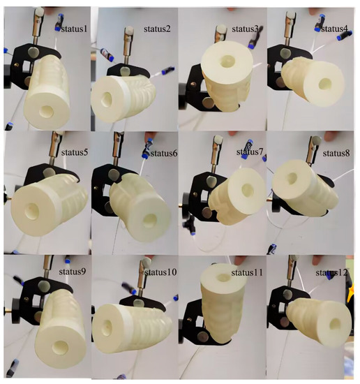
Figure 16.
Actual deformation effect of flexible joint.
Table 7.
Deformation analysis.
As can be seen from Table 7, 100 kPa gas pressure is injected into channels 1, 2, 3, and 4 from state 1 to state 4, the joint deforms to the positive direction of the Y axis, the positive direction of the X axis, the negative direction of the Y axis, and the negative direction of the X axis, respectively, with a deformation amount of 10 mm. States 5~8 are the joint channel combined into 100 kPa gas pressure. The soft joint deformation to the first quadrant, the second quadrant, the third quadrant, and the fourth quadrant of the diagonal direction of deformation is 10 mm. According to the size of the gas pressure through the two channels to determine whether the bulging tip is biased to the X axis or Y axis, if the gas pressure through the two channels is the same, the joint will undergo convex deformation in the direction of the quadrant angular bisector. In states 9 to 12, based on states 1 to 4, −50 kPa gas pressure is applied, and the deformation of soft joints is 13.5 mm. The bulging deformation effect is enhanced.
To test the relationship between gas pressure and joint deformation and the degree of bending deformation in different deformation directions, an embedded pneumatic network channel is selected in the experimental flexible joint, and embedded pneumatic network channel 1 is set in this experiment. The pressure-reducing valve controls the pressure gradient of input channel 1, as shown in Figure 17.
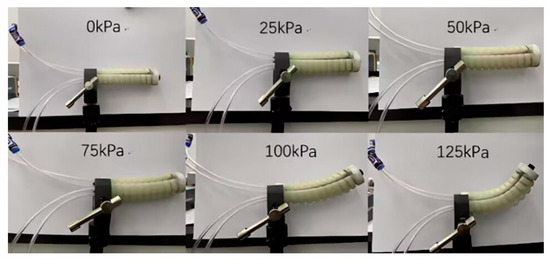
Figure 17.
Flexural degree of flexible joint under different air pressure.
The resistance values fed back by bending sensors of different gas pressures in Table 8 are converted into bending angles through the related images of bending sensor resistance values and bending angles, as shown in Figure 18a. Then the bending angle is converted into the deformation amount through Equation (7) to obtain the image between the gas pressure and the experimental deformation amount, as shown in Figure 18b.
Table 8.
Resistance values of bending sensors with different gas pressures.
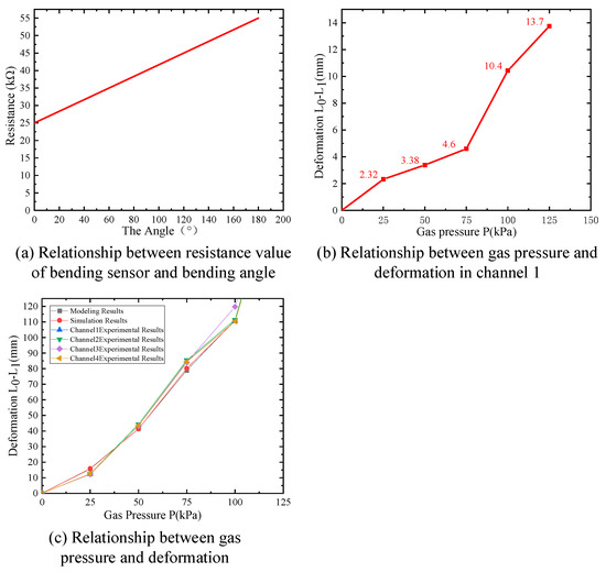
Figure 18.
Deformation correlation graph.
It can be seen from Figure 18b that the deformation of the experimental flexible joint gradually increases with the gas pressure increase, and its change trend is basically the same as the modeling and simulation results. Using the above method of verifying the relationship between gas pressure and deformation of channel 1, the relationship between gas pressure and deformation of channel 2, channel 3 and channel 4 can be obtained similarly. The relationship between gas pressure and deformation in theory, simulation, and test results is compared, as shown in Figure 18c.
It can be seen from the figure that the relationship between gas pressure and deformation of channel 2, channel 3 and channel 4 has the same change trend as the relationship image of channel 1, and the deformation of experimental flexible joints gradually increases with the increase of gas pressure. In the comparison of theory, simulation, and test results, the deformation of soft joints gradually increases with the increase of gas pressure. The change trend is consistent, and the test results are consistent with the modeling and simulation results.
5.1.2. Variable Stiffness Test
To analyze the effect of variable stiffness on the bearing capacity of soft body joints, the test setup equates the variable stiffness structure to a simple support beam structure, hangs a stage at the midpoint of the joint, and places weights to apply a constant force to measure the bending angle of the joint through the bending sensor. The relation between the bending angle, , and the elastic modulus, , of the flexible joint is:
where is the concentrated force, namely the gravity of the weight, is the length of the flexible joint, and is the moment of inertia. According to Equation (18), the larger the flexural angle of the test flexible joint is, the smaller is the elastic modulus, and the smaller is the stiffness. According to the above principles, the influence of different applied currents on the stiffness characteristics is analyzed.
Use crab clamps to restrain both ends of the flexible joint to align it in a horizontal position, record its initial position without load through the bending sensor, and then adjust the resistance values of the rheostat to 60 , 70 , 80 , 90 , 100 , and 110 , respectively, place 1 kg and 2 kg weights on the stage, and after it is stabilized record the final position of the flexible joint after the load is applied by the bending sensor to obtain the flexible joint bending angle under different loads. Figure 19a shows the state before the flexible joint becomes stiff, and Figure 19b is the state after the flexible joint becomes stiff.
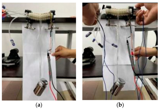
Figure 19.
Experimental setup before and after variable stiffness. (a) Before changing stiffness; (b) after varying stiffness.
By converting the rheostat resistance into applied current through the relationship between electromagnet resistance and current, the bending angle of flexible joints with 1 kg load and 2 kg load under different applied currents can be obtained, and the result is shown in Figure 20.
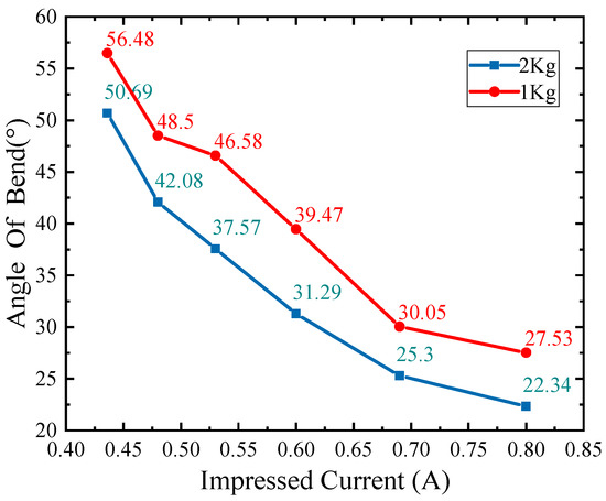
Figure 20.
The relationship between applied current and flexible joints bending angle under different loads.
As can be seen from Figure 20, the bending angle is approximately linear with the change of applied current. When the load is 1kg, and the applied current is 0.47 A to 0.57 A, the bending angle changes gently. With the increased applied current, the weak joint’s bearing capacity and bending strength are enhanced. With the applied current’s rise, the flexible joint’s bending angle gradually decreases. The stiffness effect gradually increases, consistent with the theoretical results.
6. Conclusions
In this paper, a pneumatic modular joint with full deformation and dynamic stiffness adjustment is designed and fabricated. Its deformation and variable stiffness characteristics are analyzed theoretically, simulated and experimentally, and the rigid-flexible coupling characteristics of the soft joint are revealed. Specific conclusions are as follows:
- (1)
- The deformation and variable stiffness models are established, and the gas pressure and deformation amount, and the correspondence between the magnetic field strength and the stiffness of the drive module, are obtained.
- (2)
- Through finite element simulation analysis, the change law of pressure and deformation under different stiffness conditions is obtained, and the change law of magnetic field strength and joint stiffness under different deformation conditions is considered.
- (3)
- Experiments verify the theoretical analysis, and the experiments show that, under the simultaneous action of deformation and variable stiffness, the compliance and bearing capacity are taken into account, and the experimental results of the drive module are in good agreement with the calculation and simulation results of the theoretical model.
Author Contributions
Conceptualization, S.L. and Y.B.; methodology, S.L.; software, Y.D.; validation, Y.B. and J.Z.; formal analysis, H.S.; investigation, S.L.; resources, S.L.; data curation, Y.B.; writing—original draft preparation, Y.B.; writing—review and editing, S.L.; visualization, Z.C. and X.C.; supervision, S.L.; project administration, H.S.; funding acquisition, S.L. and C.A. All authors have read and agreed to the published version of the manuscript.
Funding
This research was supported by the National Natural Science Foundation of China (Nos. 52275069 and 52175065), the Hebei Natural Science Foundation (No. E2022203041) and the Bureau of Science and Technology of Hebei Province, China, grant number (No. E2021203020).
Data Availability Statement
No new data were created.
Conflicts of Interest
The authors declare no conflict of interest.
References
- Xu, F.-Y.; Jiang, F.-Y.; Jiang, Q.-S.; Lu, Y.-X. Soft Actuator Model for a Soft Robot with Variable Stiffness by Coupling Pneumatic Structure and Jamming Mechanism. IEEE Access 2020, 8, 26356–26371. [Google Scholar] [CrossRef]
- Gilday, K.; Hughes, J.; Iida, F. Wrist-driven passive grasping: Interaction-based trajectory adaption with a compliant anthropomorphic hand. Bioinspir. Biomim. 2021, 16, 026024. [Google Scholar] [CrossRef] [PubMed]
- Zhou, P.; Yao, J.; Zhang, S.; Wei, C.; Zhang, H.; Qi, S. A bioinspired fishbone continuum robot with rigid-flexible-soft coupling structure. Bioinspir. Biomim. 2022, 17, 066012. [Google Scholar] [CrossRef]
- Chen, J.; Jin, H.; Iida, F.; Zhao, J. A design concept of parallel elasticity extracted from biological muscles for engineered actuators. Bioinspir. Biomim. 2016, 11, 056009. [Google Scholar] [CrossRef]
- Wockenfu, W.R.; Brandt, V.; Weisheit, L.; Drossel, W.-G. Design, Modeling and Validation of a Tendon-Driven Soft Continuum Robot for Planar Motion Based on Variable Stiffness Structures. IEEE Robot. Autom. Lett. 2022, 7, 3985–3991. [Google Scholar] [CrossRef]
- Wang, Y.; Yang, X.; Chen, Y.; Wainwright, D.K.; Kenaley, C.P.; Gong, Z.; Liu, Z.; Liu, H.; Guan, J.; Wang, T.; et al. A biorobotic adhesive disc for underwater hitchhiking inspired by the remora suckerfish. Sci. Robot. 2017, 2, eaan8072. [Google Scholar] [CrossRef]
- Gu, G.; Zou, J.; Zhao, R.; Zhao, X.; Zhu, X. Soft wall-climbing robots. Sci. Robot. 2018, 3, eaat2874. [Google Scholar] [CrossRef]
- Seok, S.; Onal, C.D.; Cho, K.-J.; Wood, R.J.; Rus, D.; Kim, S. Meshworm: A peristaltic soft robot with antagonistic nickel titanium coil actuators. IEEE/ASME Trans. Mechatronics 2012, 18, 1485–1497. [Google Scholar] [CrossRef]
- Kashima, S.; Miyasaka, F.; Hirata, K. Novel soft actuator using magnetorheological elastomer. IEEE Trans. Magn. 2012, 48, 1649–1652. [Google Scholar] [CrossRef]
- Wang, H.; Wang, C.; Chen, W.; Liang, X.; Liu, Y. Three-dimensional dynamics for cable-driven soft manipulator. IEEE/ASME Trans. Mechatron. 2016, 22, 18–28. [Google Scholar] [CrossRef]
- Sun, Y.; Zhang, Q.; Chen, X.; Chen, H. An Optimum Design Method of Pneu-Net Actuators for Trajectory Matching Utilizing a Bending Model and GA. Math. Probl. Eng. 2019, 2019, 6721897. [Google Scholar] [CrossRef]
- Niu, C.; Luan, C.; Shen, H.; Song, X.; Fu, J.; Zhang, L.; Sun, Y.; Xu, G.; Ruan, Z. Tunable soft–stiff hybridized fiber-reinforced thermoplastic composites using controllable multimaterial additive manufacturing technology. Addit. Manuf. 2022, 55, 102836. [Google Scholar] [CrossRef]
- Yang, Y.; Chen, Y.; Li, Y.; Wang, Z.; Li, Y. Novel variable-stiffness robotic fingers with built-in position feedback. Soft Robot. 2017, 4, 338–352. [Google Scholar] [CrossRef] [PubMed]
- Li, Y.; Chen, Y.; Yang, Y.; Wei, Y. Passive Particle Jamming and Its Stiffening of Soft Robotic Grippers. IEEE Trans. Robot. 2017, 33, 446–455. [Google Scholar] [CrossRef]
- Huang, L.; Hu, H.; Ouyang, Q. Design and Feasibility Study of MRG–Based Variable Stiffness Soft Robot. Micromachines 2022, 13, 2036. [Google Scholar] [CrossRef]
- Konda, R.; Bombara, D.; Swanbeck, S.; Zhang, J. Anthropomorphic Twisted String-Actuated Soft Robotic Gripper with Tendon-Based Stiffening. IEEE Trans. Robot. 2022, 39, 1178–1195. [Google Scholar] [CrossRef]
- Shiva, A.; Stilli, A.; Noh, Y.; Faragasso, A.; De Falco, I.; Gerboni, G.; Cianchetti, M.; Menciassi, A.; Althoefer, K.; Wurdemann, H.A. Tendon-Based Stiffening for a Pneumatically Actuated Soft Manipulator. IEEE Robot. Autom. Lett. 2016, 1, 632–637. [Google Scholar] [CrossRef]
- Crowley, G.B.; Zeng, X.; Su, H.-J. A 3D Printed Soft Robotic Gripper with a Variable Stiffness Enabled by a Novel Positive Pressure Layer Jamming Technology. IEEE Robot. Autom. Lett. 2022, 7, 5477–5482. [Google Scholar] [CrossRef]
- Zhao, Y.; Shan, Y.; Guo, K.; Han, L.; Qi, L.; Yu, H. Principle and Performance Analysis of Soft Continuum Robot with Large Range Variable Stiffness Based on Spherical Particles. In Proceedings of the 2019 IEEE 9th Annual International Conference on CYBER Technology in Automation, Control, and Intelligent Systems (CYBER), Suzhou, China, 29 July–2 August 2019; pp. 719–724. [Google Scholar]
- Al Abeach, L.A.; Nefti-Meziani, S.; Davis, S. Design of a Variable Stiffness Soft Dexterous Gripper. Soft Robot. 2017, 4, 274–284. [Google Scholar] [CrossRef]
- Al Abeach, L.; Nefti-Meziani, S.; Theodoridis, T.; Davis, S. A Variable Stiffness Soft Gripper Using Granular Jamming and Biologically Inspired Pneumatic Muscles. J. Bionic Eng. 2018, 15, 236–246. [Google Scholar] [CrossRef]
- Li, Y.; Ren, T.; Chen, Y.; Chen, M.Z. A variable stiffness soft continuum robot based on pre-charged air, particle jamming, and origami. In Proceedings of the 2020 IEEE International Conference on Robotics and Automation (ICRA), Paris, France, 31 May–31 August 2020; pp. 5869–5875. [Google Scholar]
- Wang, T.; Zhang, J.; Li, Y.; Hong, J.; Wang, M.Y. Electrostatic Layer Jamming Variable Stiffness for Soft Robotics. IEEE/ASME Trans. Mechatron. 2019, 24, 424–433. [Google Scholar] [CrossRef]
- Liu, Z.; Wang, Y.; Wang, J.; Fei, Y.; Du, Q. An obstacle-avoiding and stiffness-tunable modular bionic soft robot. Robotica 2022, 40, 2651–2665. [Google Scholar] [CrossRef]
- Luo, Y.; Wright, M.; Xiao, Q.; Yue, H.; Pan, G. Fluid–structure interaction analysis on motion control of a self-propelled flexible plate near a rigid body utilizing PD control. Bioinspir. Biomim. 2021, 16, 066002. [Google Scholar] [CrossRef] [PubMed]
- Wang, C.; Tang, H.; Zhang, X. Fluid-structure interaction of bio-inspired flexible slender structures: A review of selected topics. Bioinspir. Biomim. 2022, 17, 041002. [Google Scholar] [CrossRef]
- Stano, G.; Ovy, S.a.I.; Percoco, G.; Zhang, R.; Lu, H.; Tadesse, Y. Additive Manufacturing for Bioinspired Structures: Experimental Study to Improve the Multimaterial Adhesion Between Soft and Stiff Materials. 3D Print. Addit. Manuf. 2023; ahead of print. [Google Scholar] [CrossRef]
- Shan, Y.; Zhao, Y.; Pei, C.; Yu, H.; Liu, P. A novel design of a passive variable stiffness soft robotic gripper. Bioinspir. Biomim. 2022, 17, 066014. [Google Scholar] [CrossRef]
- Sun, W.; Yu, J.; Cai, Y. Influence of magnetic field, magnetic particle percentages, and particle diameters on the stiffness of magnetorheological fluids. J. Intell. Mater. Syst. Struct. 2020, 31, 2312–2325. [Google Scholar] [CrossRef]
- Ilievski, F.; Mazzeo, A.D.; Shepherd, R.F.; Chen, X.; Whitesides, G.M. Soft robotics for chemists. Angew. Chem. Int. Ed. 2011, 50, 1890–1895. [Google Scholar] [CrossRef]
- Yap, H.K.; Ng, H.Y.; Yeow, C.-H. High-Force Soft Printable Pneumatics for Soft Robotic Applications. Soft Robot. 2016, 3, 144–158. [Google Scholar] [CrossRef]
- Liu, S.Y.; Zhang, J.T.; Wang, J.; Deng, Y.J.; Xin, C.T. Design and simulation analysis of fluid-driven modular soft body bionic elephant trunk joint variable stiffness structure. Hydraul. Pneum. 2022, 46, 152–158. [Google Scholar]
- Zhang, Y.; Chen, W.; Chen, J.; Cheng, Q.; Zhang, H.; Xiang, C.; Hao, L. Stiffness Analysis of a Pneumatic Soft Manipulator Based on Bending Shape Prediction. IEEE Access 2020, 8, 82227–82241. [Google Scholar] [CrossRef]
- Taniguchi, H.; Miyake, M.; Suzumori, K. Development of new soft actuator using magnetic intelligent fluids for flexible walking robot. In Proceedings of the ICCAS 2010, Gyeonggi-do, South Korea, 27–30 October 2010; pp. 1797–1801. [Google Scholar]
- Xuan, T.; Li, J.; Li, B.; Fan, W. Effects of the non-uniform magnetic field on the shear stress and the microstructure of magnetorheological fluid. J. Magn. Magn. Mater. 2021, 535, 168066. [Google Scholar] [CrossRef]
Disclaimer/Publisher’s Note: The statements, opinions and data contained in all publications are solely those of the individual author(s) and contributor(s) and not of MDPI and/or the editor(s). MDPI and/or the editor(s) disclaim responsibility for any injury to people or property resulting from any ideas, methods, instructions or products referred to in the content. |
© 2023 by the authors. Licensee MDPI, Basel, Switzerland. This article is an open access article distributed under the terms and conditions of the Creative Commons Attribution (CC BY) license (https://creativecommons.org/licenses/by/4.0/).