Abstract
This article serves as a continuation of our previously published work and focuses on loose material transport via sandwich belt conveyors. Experimental, analytical, stochastic, and numerical approaches are used to obtain and utilize the moduli of a bilateral Winkler elastic foundation that represent a loose material, which is wheat (Triticum aestivum) that is free of bran in this case. The solutions were obtained for a uniformly and nonuniformly distributed loose material. The task of the conveyor with loose material is simplified into a symmetric task, i.e., a beam on an elastic bilateral Winkler foundation, for an analytical solution and stochastic solution (Anthill and Matlab sw). In a numerical approach, this is considered a plane strain problem within the finite element method (Ansys and MSC.Marc sw). The experimental data are evaluated and used to obtain the functions of Winkler elastic foundation moduli, which are further considered in the numerical solution. The finite element method mainly serves as a verification tool. The acquired histograms of the elastic foundation moduli can be further applied in various scientific and research fields.
Keywords:
sandwich belt conveyor; belt; wheat; Triticum aestivum; loose material; uniform distribution; non-uniform distribution; Winkler elastic foundation; beams; analytical approach; theory of 2nd order in mechanics; plane strain formulation; FEM; small deformations; large deformations; stochastic approach; Monte Carlo method; Newton–Raphson method 1. Introduction
In today’s world, there is still a great need for the transportation of various materials. Therefore, the focus of our article is on belt conveyors, namely, sandwich belt conveyors, which can transport material in general directions of movement. The VSB—Technical University of Ostrava, Faculty of Mechanical Engineering developed and built its own sandwich belt conveyor that is suitable for research and teaching. This sandwich belt conveyor was used in this article [1,2,3,4].
This article extends and builds upon our previous work [5], which focused on the use of an elastic foundation in the transport of wheat via sandwich belt conveyors, and this task was perceived as a static one. An EP500 cord conveyor belt, composed of rubber, was tested in the horizontal and vertical directions.
The solutions were obtained experimentally, analytically, and stochastically (probabilistic Monte Carlo method) for a bilateral Winkler elastic foundation by utilizing two thickness layers of uniformly and nonuniformly distributed loose material, i.e., dry wheat (Triticum aestivum) that was free of bran. The deflection of the belt with wheat and the horizontal and vertical loading forces were measured as the basic values for the subsequent evaluation. The loading was conducted by externally applying loads onto pressure rollers with a diameter of d = 0.05 m. The moduli of the elastic foundation were determined from the measurements for the different thicknesses of wheat layers between the covering and carrying belts. The analytical solution was based on the experimental measurements that were carried out with our original testing device, as shown in Figure 1 and Figure 2 and described in [5].
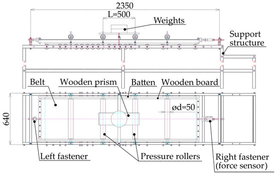
Figure 1.
Our device for measuring the deflection of a layer of loose material from the applied pressure force of a conveyor roller on a pressure belt; dimensions are in mm [5].
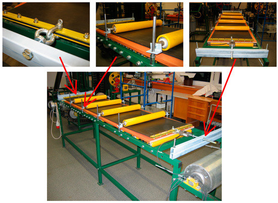
Figure 2.
The implemented functional sample, which is called the “laboratory device for measuring the transformation of a loose material layer from the applied pressure force of a conveyor roller on a pressure belt” [5].
Loose material transport does not usually involve uniformly distributed (spread) loose material, as in [5]; rather, the material is randomly distributed, and this problem is mainly addressed in this article.
In accordance with [5], we study the next phase of this research, which focuses on the nonuniform distribution of wheat. Loose material—specifically, wheat—is most commonly transported in clusters in common technical practice, i.e., wheat is not uniformly distributed along the width or length of the belt.
The experimental device and methodology of the calculations when applying the theory of beams on an elastic foundation (wheat) are the same as those in [5], with some small differences in details. The results are stochastically evaluated and compared with the results from the first part of our previous article [5].
In addition, finite element analysis (FEA) is newly employed by using software such as Ansys 2022R2 [6] and MSC.Marc/Mentat [7]. The finite element method (FEM) is not completely necessary; however, it is used as a tool for verifying the analytical results presented in [5].
Matlab sw [8] and Anthill sw [9] are used for regression and stochastic analyses, respectively.
The experimental, analytical, numerical, and stochastic solutions are in ample accordance.
The obtained results and presented methods can be used for the construction of sandwich rubber belt conveyors for transporting not only wheat, but also a wide variety of other loose materials (corn, gravel, soil, industrial waste, etc.), which can be distributed either uniformly or nonuniformly between the transporting belts.
The use of an elastic foundation, namely, Winkler’s bilateral model (according to the theory of the second order in mechanics), in conjunction with a sandwich belt conveyor, is sufficiently suitable and has been verified with all of the above-mentioned methods. Apart from our previous study, the original approach presented in this work has not been published elsewhere so far (see [5,10]). However, there is a large amount of literature on the theory and practice of elastic foundations and stochastic methods [11,12,13,14,15,16,17,18,19,20,21].
2. Materials and Methods
2.1. Experimental Measurement
For the purpose of obtaining the stiffness of elastic foundation /Nm−3/, an experimental measurement of the deflection of a covering belt with wheat was performed similarly to that in [5]. The measurements were performed at the sandwich belt conveyor that was proposed and built at the VSB—Technical University of Ostrava, Faculty of Mechanical Engineering.
The difference between the experimental setup and that in our previous study is that in [5], the wheat was distributed evenly (constant thickness) on the wooden board, which represented a plane of symmetry (see Figure 3 and [5]), whereas, in this study, there were new spacings of width hα /m/ and angle α /deg/ under the loading rollers (see Figure 4).
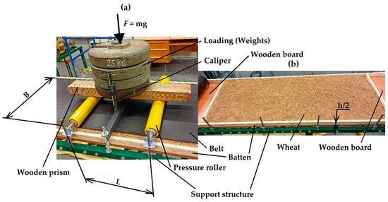
Figure 3.
(a) Measurement of deflection in the middle between rollers. (b) Even distribution of wheat; see [5].
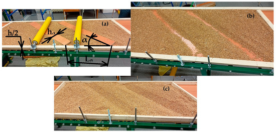
Figure 4.
Layering of wheat used in this study. (a) Creation of spacing in wheat layering, (b) spacing in wheat before loading, and (c) spacing in wheat after loading (end of the experiment).
The spacings in wheat layering provide a more realistic layout of the loose material and, thus, a better representation of wheat transport.
Wheat can be considered a loose material. Therefore, it is clear from a comparison of Figure 4a,b that the wheat repose (i.e., slide, slump) is consistent with the angle of repose. Wheat repose was caused by the removal of the battens before the experiment.
The spacings were created by using a batten beneath the pressure rollers under an angle of α = 45°, a thickness of hα = 0.036 m, and a length of Lα = 0.25 m, as shown in Figure 4a. The spacings that were created before loading are illustrated in Figure 4b. The spacings were partially filled with wheat grain after removing the battens; after loading (end of the experiment), the spacings were filled more; see Figure 4b,c.
2.2. Sandwich Conveyor Belt and Its Force Sensor
The EP500 belt used had a width of B = 0.4 m, a thickness of t = 0.009 m, and a designated Young’s modulus of Pa. The belt was reinforced by a cord. An RSC-1 T force sensor was used to measure the tensile forces /N/ in the belt. For more information, see [5].
2.3. Wheat
Wheat grains (Triticum aestivum) that were free of bran were accessible and were used for the experimental testing.
The wheat had a loose weight of ρs = 767 kg/m3—or 76.7 kg/hl—and a loose grain angle of ψd = 10°. The granularity of wheat can be defined by the largest grain length, which, in our case, was ; for more information, see [5].
2.4. Analytical Approach
The problem that was solved was basically the same as that in [5]; however, the difference between the studies is the spacing of the wheat layer (uniform vs. nonuniform distribution), as shown in Figure 4. The problem was simplified into an infinite beam (belt) task on a Winkler bilateral elastic foundation (loose material) that was loaded axially (force ) and transversally (forces /N/), as shown in Figure 5.
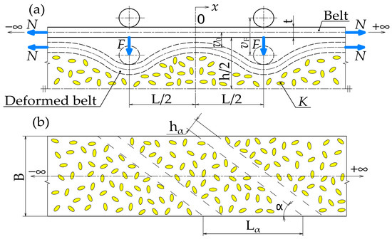
Figure 5.
Schematic drawing of the conveyor belt. (a) Front view and (b) plan view before loading with the belt and pressure rollers removed.
In Figure 5, it can be seen that the distance between loading forces, i.e., pressure rollers, was L = 0.5 m. The other dimensions can be found in Section 2.2, and the deflections of the belt with loose material in the measured places were /m/ and /m/.
The spacings will be reflected in the solution by showing different elastic foundation modulus values. However, the approach and equations will be the same as if there were no spacings.
The applied theory of infinite beams on an elastic foundation, according to Winkler, satisfies the differential equation of the theory of the second order:
where /m4/ is the principal second moment of the cross-section of the belt (), and /m/ is the deflection of the beam.
The general solution with the applied boundary conditions for this case is explained and presented in [5].
According to [5] and the boundary conditions, the specific equations and relations for the deflections, slopes, bending moments, and shearing forces midway between forces (x = 0 m) and under force (x = L/2 = 0.25 m) are given in Table 1. For more information on the derivation and boundary conditions, see [5].

Table 1.
Calculation of the quantities at the measuring points, i.e., under the force and midway between the forces according to Figure 5.
2.5. Numerical Approach
2.5.1. Finite Element Analysis
Finite element analysis is a numerical way of computing unknowns that utilizes the finite element method.
The analyses were conducted by using software such as Ansys Workbench 2022R2 and MSC.Marc/Mentat 2022.3. These software systems do not allow the use of elastic foundations in combination with beam elements. However, using FEA to simulate the same process as that for the analytical solution would be redundant and would not reveal anything new. Thus, in FEA, the task is considered as a plane problem, which is a good upgrade compared to 1D analytical problems (plane beam on elastic foundation). The plane problem is treated as generalized plane strain (Ansys sw) and plane strain (MSC.Marc sw).
Finite element software generally does not allow the modeling of infinitely long structures, as was performed for the analytical solution presented in Section 2.3. Although, theoretically, the response of the beam to loading will become zero in infinity, practically, it can be considered zero much earlier; thus, it is not necessary to have an infinitely long model. Consequently, the finite length of the belt introduces negligible error in FEM compared to that in analytical solutions.
Linear theory of small deformations and nonlinear theory of large deformations were applied in FEA.
The material properties of the belt are described in Section 2.2.
The main goal of FEA is to verify analytical results; thus, the values of foundation moduli that were obtained from the analytical solution were input into the FE software. The displacement outputs from FEA were observed and compared with the measured values for uniformly distributed wheat from [5]. If the calculated displacements significantly differed from the measured values, a comparison was also conducted for the nonuniformly distributed wheat discussed in this article, and appropriate conclusions were drawn.
2.5.2. Finite Element Meshes and Their Boundary Conditions
The models had a length of 1 m, and the other parameters are presented in Table 2. The dimensions were proven sufficient by conducting a mesh convergence study with the so-called h-method. The h-method is based on decreasing the finite element size and comparing the results—in this case, displacements—with those of the previous mesh. Both FE models were based on plane quadratic quadrilateral elements with eight nodes and two degrees of freedom in each node, i.e., the nodal displacements that were calculated in the X and Y directions.

Table 2.
Information about the FE mesh.
The finite element model in Ansys sw exhibited fewer nodes/elements because it was mostly used to compare the results with those of MSC.Marc sw and accelerate the calculations. For these reasons, the mesh was satisfactory.
The Ansys solution was used more out of curiosity and as a supplement to or confirmation of the MSC.Marc results. As previously mentioned, Ansys sw had a slightly different planar definition for our problem.
The mesh and boundary conditions for MSC.Marc sw are shown in Figure 6 and Figure 7, and the same boundary conditions were also applied in Ansys sw. However, the boundary conditions are only shown on MSC.Marc/Mentat.
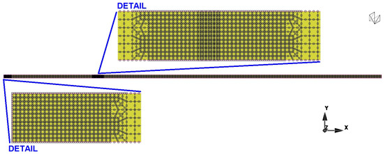
Figure 6.
Finite element mesh and its details (MSC.Marc/Mentat sw).

Figure 7.
Boundary conditions (MSC.Marc/Mentat sw).
According to Figure 7, on the left side of the belt, there was a symmetric boundary condition (“SYMMETRY”), i.e., the displacement in the X direction was zero. At a distance of L/2 = 0.25 m from this symmetric boundary condition, there was a point transverse force (“FORCE_F”) applied along the cross-section. On the right side, there was a tensile force (“FORCE_N”). At the bottom edge of the model, there was an elastic foundation with a stiffness of (“ELASTIC_FOUNDATION”).
2.6. Regression
Similarly to [5], the Matlab 2021b software was used for statistical processing and regression of the values of the elastic foundation modulus . Due to the variance in the results, the dependence values were calculated for a defined h of 36 and 72 mm ( and ), where a, b /m−3/, and c /Nm−3/ were the regression constants.
Statistical processing was performed in Matlab by using the “Curve Fitting Toolbox”. For more information, see, e.g., [5,8].
2.7. Monte Carlo Method
As in [5], a modern probabilistic (stochastic) approach based on the Monte Carlo method was used.
As described in [5], the Anthill software was used, which also included a pseudo-random number generator. In the Anthill software, the period of the pseudo-random number generator is 232. The Anthill software uses bounded (truncated) histograms as inputs and outputs. A histogram is an approximate representation of the distribution of the numerical data. The Anthill program allows for the evaluation and display of multidimensional (multicomponent) random variables. For more information, see, e.g., [9].
The Anthill program was used to process statistical data and histograms in connection with the calculations of the elastic moduli .
For more information, see [5].
3. Results
3.1. Finite Element Analyses—Results for a Uniform Layer of Wheat and Verification of the Results of [5]
FEA was used for the above-mentioned results [5] for the verification of the analytical and experimental results.
The primary results of the FEA that were evaluated were the displacements under force for both the linear theory of small deformations and the nonlinear theory of large deformations. These results were then compared with the analytical values obtained for the beam model on the elastic foundation.
According to Section 2.5, the sandwich belt was analyzed with FEM. The experimental results presented in [5], i.e., /Nm−3/, for the Winkler moduli of elasticity acquired from the measurement of under force were applied as inputs in FEM.
An example of the calculated deflection for the chosen measured values (, , ) from both Marc and Ansys sw is shown in Figure 8 and Figure 9.
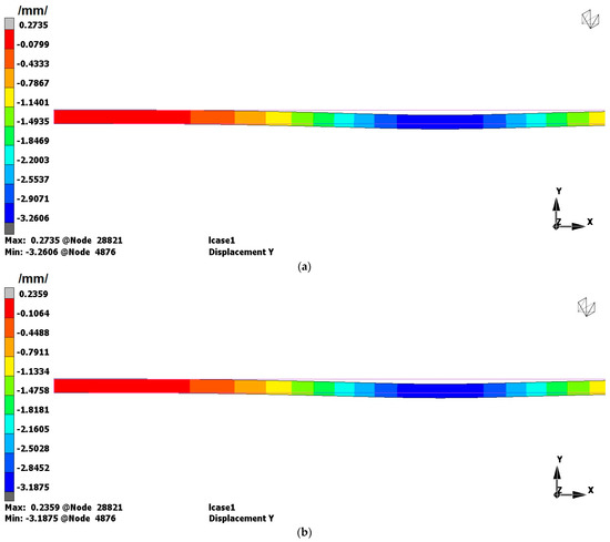
Figure 8.
Displacement in the Y direction for the original and deformed belt acquired from MSC.Marc sw for , , and . (a) Results for the linear theory of small deformations. (b) Results for the nonlinear theory of large deformations.
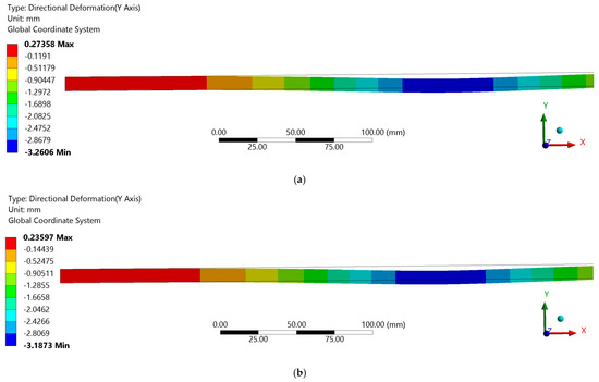
Figure 9.
Displacement in the Y direction for the original and deformed belt acquired from Ansys sw for , , and . (a) Results for the linear theory of small deformations. (b) Results for the nonlinear theory of large deformations.
The second results to be evaluated were axial stresses. Since the stresses were not calculated in the analytical solution and we had nothing with which to compare them, we only show the results from MSC.Marc sw for the same inputs as those that were chosen for the displacements (, , and ), as shown in Figure 10.
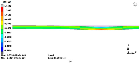
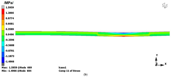
Figure 10.
Axial stress distribution for the original and deformed belt acquired from MSC.Marc sw for , , and . (a) Results for the linear theory of small deformations. (b) Results for the nonlinear theory of large deformations.
Comparison of the FEA and Analytical Results
The results of the Ansys and Marc software slightly differed, and this was due to the different finite element meshes, as well as the somewhat different definitions of the plane deformation formulations. Since the results of the Marc software were calculated for a larger number of elements (denser mesh), they were used to process the following results.
A comparison of the measured displacements and calculated displacements by using FEM, i.e., deflections under force , was conducted tabularly and graphically for uniformly distributed layers of wheat with a layer thickness of h = 72 mm, as described in [5] and shown in Table 3 and Figure 11, Figure 12, Figure 13 and Figure 14.

Table 3.
Comparison of the experimental and numerical deflections for the uniform thickness of the wheat layer of h = 72 mm according to Figure 3.
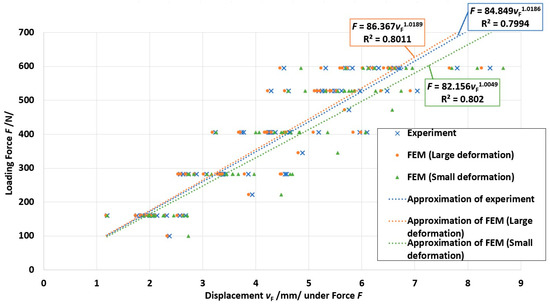
Figure 11.
Graphical comparison of the experimental and numerical results. Dependence of the loading force on the displacement .
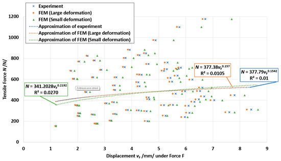
Figure 12.
Graphical comparison of the experimental and numerical results. Dependance of the tensile force on the displacement .
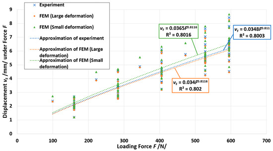
Figure 13.
Graphical comparison of the experimental and numerical results. Dependence of the displacement on the loading force .
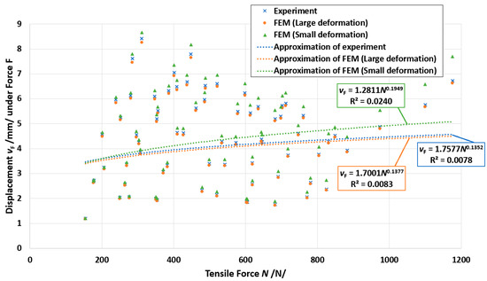
Figure 14.
Graphical comparison of the experimental and numerical results. Dependence of the displacement on the tensile force .
The values of deflection (under force ) presented in Table 3 were calculated from the arithmetic mean of four measurements in four places (at each end of the two pressure rollers). These measurements were performed with calipers.
The calculations of the FEM error for small and large deformations are given by Equation (2).
The definition of error in Equation (2) is actually a kind of definition for discrepancies between the analytical and numerical values.
According to Table 3, the FEM errors for small deformations were from −15.17% to 0.39%, and the FEM errors for large deformations were from 1.44% to 2.10%. The FEM errors were mainly caused by the values of , which were calculated from the different analytical calculations of the beam on an elastic foundation, and they were marginally due to discretization errors. The largest errors were for small deformations because they were the furthest from the second beam theory of the analytical model.
However, FEM confirmed the validity of using beams on an elastic foundation for modeling sandwich belts.
The FEM calculations that used the large deformation theory were more appropriate than those that used the theory of small deformations. Hence, our analytical approach was in good concordance with the FEM solution of large deformations.
From Table 3, it is evident that the tensile force had a smaller effect on deflection when applying the linear theory of small deformations compared to that obtained when applying the nonlinear theory of large deformations. This came from the fact that the deflection for small deformations was larger than both the experimental and numerical values for large deformations. However, the displacements from the nonlinear theory of large deformations were often closer to the measured values than the displacements from the linear theory of small deformations. The measured displacement always lay between the two numerical values.
A graphical comparison of the numerical and measured displacements was conducted in the form of and or and , wherein the measured and calculated values were approximated with power functions in Excel sw, as shown in Figure 11, Figure 12, Figure 13 and Figure 14.
The coefficient of determination R2 was approximately 0.8 for , as shown in Figure 11; for , it approached approximately 0.01, as shown in Figure 12. The coefficient of determination R2 was also approximately 0.8 for as shown in Figure 13; for , it also approached approximately 0.01, as shown in Figure 14. This led to the conclusion that the tensile force had much larger variance than the loading force . The goal was not to look for regressions connected with , but rather to look for possible correlations. Correlations are useful for describing simple relationships among data. According to our results, there was better correlation between and than between and .
The results show that the loading force exerted the greatest influence on the deflection of the beam and that the experimental results correlated very well with FEM, especially when applying the theory of large deformations.
3.2. Nonuniform Layer of Wheat
This subchapter deals with the evaluation of a nonuniform layer of wheat with the same layer thicknesses as in our previous article [5], i.e., h = 72 mm and h = 36 mm, as shown in Figure 4. The experiments are described in Section 2.1, the belt is described in Section 2.2, and the wheat is described in Section 2.3.
To calculate the unknowns, namely, the Winkler moduli of the elastic foundation, the Newton–Raphson method was used; see, e.g., [5,22] and the Matlab code provided in Table 4. The values obtained for the Winkler moduli of the foundation and are presented in Table 5 and Figure 15 and Figure 16. Table 5 only contains the results from the measurements and calculations for h = 72 mm; for h = 36 mm, the results were similar and, thus, not necessary to list here.

Table 4.
Matlab script for calculating Winkler moduli of the elastic foundation.

Table 5.
Winkler moduli of the foundation and /Nm−3/ for individual measurements for the thickness of the nonuniform wheat layer (h = 72 mm) according to Figure 4.
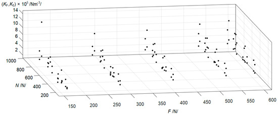
Figure 15.
Relationship of /Nm−3/ for the nonuniform wheat layer thickness of h = 72 mm (see the results in Table 5).
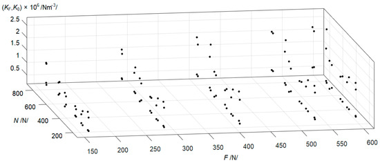
Figure 16.
Relationship of /Nm−3/ for the nonuniform wheat layer thickness of h = 36 mm.
3.2.1. Approximation of Results
According to Section 2.6, the moduli of the foundation calculated for the nonuniform distribution were fitted by using a linear approximation function in the form of , where /m−3/, and /Nm−3/ were regression constants. This simple plane function with the independent variables and was shown to be among the best fits for the given data. The approximations from Matlab for h = 72 mm () and h = 36 mm () are illustrated in Figure 17 and Figure 18 with three different views.
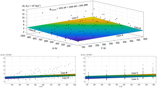
Figure 17.
Data approximated (median values) with the linear function for nonuniformly distributed wheat with a layer thickness of h = 72 mm.
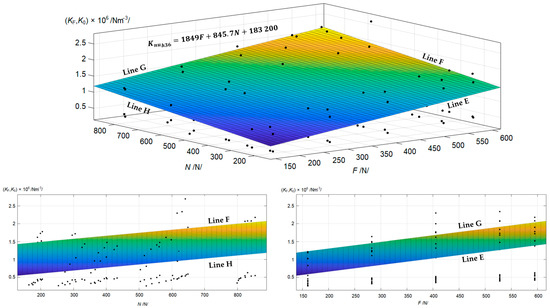
Figure 18.
Data approximated (median values) with the linear function for nonuniformly distributed wheat with a layer thickness of h = 36 mm.
“Line A” to “Line H” in Figure 17 and Figure 18 mark the borders of the assumed approximation functions and are present to make the figures with 2D histograms easier to read.
The median value relations of Equations (3) and (4) for nonuniformly distributed wheat were obtained with Matlab and the values in Figure 17 and Figure 18:
For further comparison, the approximation functions for the median values for uniformly distributed wheat could be calculated by using Equations (5) and (6) (see [5]):
The trend of the approximations remained similar for the uniform and nonuniform distributions of wheat, namely, the loading force had a larger effect on the modulus of the foundation than that of the tensile force .
When comparing the nonuniform and uniform distributions of wheat for the same layer thickness, it was evident that the modulus of the foundation was lower if there were spacings in the wheat distribution.
From a comparison of Equation (3) with Equation (5), it could be concluded that Equation (3) provided 2.23 to 2.75x smaller values of the foundation modulus. As shown by a comparison of Equation (4) with Equation (6), the constants multiplying and were similar across the uniformity/nonuniformity of the wheat distribution; however, the last constant was an order of magnitude lower for the nonuniform distribution than that for the uniform distribution of wheat. This would make it appropriate to study experiments with different spacings (e.g., ) and thicknesses h in the future.
3.2.2. Stochastic Evaluation
The stochastic processing of the obtained results was performed with the Anthill software (version 2.6 Pro) [9] by utilizing the same process as that in [5].
From the analytical (see Table 4) and approximated (see Figure 17 and Figure 18 and Equations (3) and (4)) values, an error was calculated:
where /Nm−3/ is the analytical Winkler modulus of the foundation ( and ), as shown in Table 5, and /Nm−3/ is the function value of the Winkler foundation modulus; see Equations (3) and (4), as well as [5].
The error was used to calculate the standard deviation of the normal distribution. The normal distribution best describes the randomness in nature and, hence, is considered here. The standard deviation for h = 72 mm was ; for h = 32 mm, it was (for uniform layering, the values were and ; see [5]). These values were used to construct truncated normal histograms on defined intervals, i.e., and , as shown in Figure 19.

Figure 19.
Truncated normal histograms /1/ and /1/ (Anthill sw).
The histograms were then used to stochastically multiply the approximated functions (3) and (4) in order to obtain a wider range of results that would better incorporate reality, i.e., randomness:
Equations (8) and (9) are shown in Figure 20 as 2D histograms. The forces and were considered with a uniform distribution ranging from 0 to 1000 N. To create the 2D histograms, 106 pseudo-random simulations were run in Anthill sw.
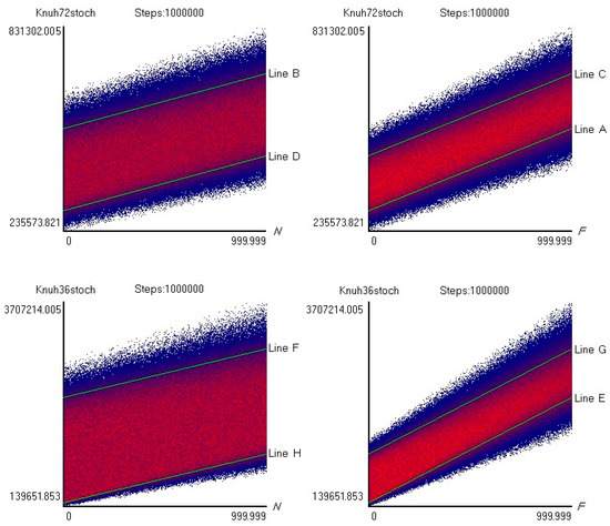
Figure 20.
The 2D histograms (top) /Nm−3/ and (bottom) /Nm−3/ from Anthill sw.
“Line A” to “Line H” in Figure 20 are the same as those in Section 3.2.1, as shown in Figure 17 and Figure 18.
4. Discussion
The results of the first part of this research, which focused on the transportation of uniformly distributed wheat that was free of bran by using a cord rubber belt of a sandwich conveyor (as described in [5]), and the results published in this article, which focused on the transportation of nonuniformly distributed wheat that was free of bran by using the same conveyor system, provide the following conclusions:
- Experiments were performed by using the laboratory test equipment in our department, i.e., a conveyor with a cover belt and pressure rollers, as shown in Figure 1, Figure 2, Figure 3 and Figure 4. The original measurements—specifically, those of the compression of the belt with wheat (Triticum aestivum)—were conducted for two thicknesses of loose material, namely, h = 72 mm and h = 36 mm, by using symmetric boundary conditions. The measurements were performed for uniformly distributed layers of wheat (see [5]) and nonuniformly distributed layers of wheat (presented in this article).
- Analytical models of a beam on a bilateral Winkler elastic foundation, according to the theory of the second order in mechanics, are suitable and simple enough for modeling the interaction between the belt and wheat. A relatively “simple” linear mechanics problem was then analytically solved. The cover belt was treated as a beam, the pressure rollers were replaced by point forces along the cross-section, and the interaction with the wheat was modeled as a bilateral Winkler elastic foundation.
- The finite element method confirmed the validity of the above-mentioned analytical approach. The application of the plane strain formulation was very close to our analytical model.
- The Winkler moduli of the elastic foundation were obtained from the measured data by using the Newton–Raphson method. The experiment and its evaluation showed that the Winkler modulus of elasticity was not constant, and it was influenced by several factors that were mentioned above, but the values were in the same range as those commonly reported in the literature for loose materials or elastic foundations; see, e.g., [12].
- Furthermore, the obtained results were statistically evaluated. The obtained regression plane functions were in the forms of and for the uniform distribution and of and for the nonuniform distribution of wheat. The functions were then stochastically processed in the form of defined histograms (truncated normal distribution). From the calculated values, a relatively large but natural degree of variability was found. A comparison of the median values for the moduli of the elastic foundation is presented in Figure 21.
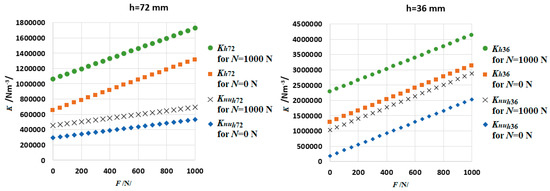 Figure 21. Comparison of the median values for the moduli of the elastic foundation on forces and .
- All approaches, i.e., experimental, analytical, numerical, and stochastic, complemented each other and were not contradictory. However, the analytical approach was easy to apply.
- Similarly, as mentioned in [5], in future work, some other characteristics could be added to the measurements; for example, a more proper and complicated model of an elastic foundation could be used for the evaluation of the interaction of the belt and loose material.
- These elastic foundation models are, e.g., the Hetényi model, which was firstly and marginally used by the authors in [10]; see also [23,24]. The differential equation for the Winkler model is prescribed via Equation (1), and the differential equation for the Hetényi (two-parameter) model is Equation (10):where /Nm−3/ and /Nm/ are the moduli of the Hetényi elastic bilateral foundation. Other two-parameter elastic foundation models can also be used, such as those of Pasternak, Filodenko-Borodic, Kerr, etc. [25,26,27]. Multi-parameter models are better suited for the behaviors of elastic foundations but are more complicated.
- Similarly, as cited in [5], the analytical model that used the beam theory and plane strain numerical FEM models could be transformed into a more complicated shell or 3D models, and other stochastic or dynamic (e.g., the start-up, steady-state, modal analysis, etc. (see, e.g., [28])) solutions can be used; see, e.g., [15,16,17,18,19,20,21,29,30,31,32,33,34,35].
- Similarly, as cited in [5], the methodology and the experimental equipment that were shown and used can also be used for different types of loose materials, e.g., seeds, sand, sawdust, gravel, industrial waste, etc., when designing belt conveyors and in material transport.
- The experiments were performed for multiple magnitudes of forces , their corresponding measured tensile forces different thicknesses h of layers of loose material, and different thicknesses of batten hα (the spacings defined in the wheat distribution). Thus, some uncertainties were considered in the calculations.
- The material properties of loose materials have greater variability (statistical dispersion) in mechanical properties than the material properties of rubber belts. However, even the material properties of belts have a statistical dispersion, which was neglected in the calculations. It was assumed that the material properties of belts could be considered constant in our initial approach.
- According to [36], a sensitivity analysis can be used for quantification. However, in this article, it was not performed. The reasons for this was that the main goal of this article was to assess sandwich belt conveyors, elastic foundations, and loose materials. The theory of probability/statistics was a secondary goal. Medians, means, and standard deviations were mainly used with the application of the Monte Carlo method.
5. Conclusions
For a sandwich belt conveyor, the finite element method was used to validate the analytical accuracy when solving the interaction between a belt and loose material as a static task.
The distribution of the loose material had a crucial role in the modulus of the elastic foundation. Uniformly distributed loose material provided higher modulus values than those of nonuniformly distributed loose material, which confirmed the initial assumptions of this article.
All of the obtained regression functions were similar in nature, i.e., the loading force had a greater influence on the elastic foundation moduli than the tensile force did, as shown Figure 21 and described by Equations (3)–(6). The stiffness—or the moduli of the elastic foundation—decreased with increasing thickness h. Hence, and . With increasing forces and , the moduli of the elastic foundation increased, too.
The statistical and stochastic solutions showed that the variance in the data was lower for nonuniformly distributed wheat. The values of the elastic foundation moduli were described by the histograms.
Other approaches for scientific and research development were mentioned.
Applications of elastic foundations in transport using sandwich belt conveyors are still new. However, they offer good, sufficiently exact, and easy-to-apply analytical models.
The results acquired here can be applied not only in the design of sandwich belt conveyors, but also wherever loose material is considered as an elastic foundation. Moreover, the trend of the obtained functions should be similar to that of other loose materials, e.g., increasing the loading force increases the stiffness of the elastic foundation.
Author Contributions
Conceptualization, K.F.; Methodology, L.H.; Resources, L.H.; Software, D.Č. and M.N.; Writing—original draft, D.Č.; Writing—review and editing, D.Č. and K.F. All authors have read and agreed to the published version of the manuscript.
Funding
This work was supported by the Ministry of Education, Youth, and Sports of the Czech Republic as part of the Specific Research Project SP2023/003 (SV3403351) and the Ministry of Industry and Trade of the Czech Republic as part of the Specific Research Project CZ.01.1.02/0.0/0.0/20_321/0024559 (MP342132), by Specific Research „Application of Modern Computational and Experimental Approaches in Applied Mechanics“ (SP2023/027), and by projects CZ.02.1.01/0.0/0.0/17_049/0008441 “Innovative Therapeutic Methods of Musculoskeletal System in Accident Surgery” and CZ.02.1.01/0.0/0.0/17_049/0008407 “Innovative and additive manufacturing technology—new technological solutions for 3D printing of metals and composite materials”.
Data Availability Statement
Data is contained within the article.
Acknowledgments
This work was supported by the Ministry of Education, Youth, and Sports of the Czech Republic as part of the Specific Research Project SP2023/003 (SV3403351) and the Ministry of Industry and Trade of the Czech Republic as part of the Specific Research Project CZ.01.1.02/0.0/0.0/20_321/0024559 (MP342132), by Specific Research „Application of Modern Computational and Experimental Approaches in Applied Mechanics“ (SP2023/027), and by projects CZ.02.1.01/0.0/0.0/17_049/0008441 “Innovative Therapeutic Methods of Musculoskeletal System in Accident Surgery” and CZ.02.1.01/0.0/0.0/17_049/0008407 “Innovative and additive manufacturing technology—new technological solutions for 3D printing of metals and composite materials”.
Conflicts of Interest
The authors declare no conflict of interest.
Nomenclature
| mm | Largest wheat grain length | |
| a | m−2 | Auxiliary variable in Matlab script |
| m−3 | Regression constant | |
| B | m | Belt width |
| b | m2 | Auxiliary variable in Matlab script |
| m−3 | Regression constant | |
| Nm−3 | Regression constant | |
| d | mm | Diameter of pressure rollers |
| rad | Slope (first derivative of deflection) of a beam | |
| m−1 | Second derivative of deflection of a beam | |
| m−3 | Fourth derivative of deflection of a beam | |
| E | Pa | Young’s modulus of a belt |
| 1 | Error between analytical and approximated values of Winkler moduli of elastic foundation | |
| % | Error of FEA | |
| e | 1 | Euler’s number |
| N | Loading force | |
| FEA | Finite element analysis | |
| FEM | Finite element method | |
| h | mm | Loose material (wheat) layer thickness |
| m | Thickness of batten (defined spacings in wheat distribution) | |
| 1 | Truncated normal histogram created from | |
| 1 | Truncated normal histogram created from | |
| m4 | Principal second moment of cross-sectional area of a belt | |
| Nm−3 | Winkler modulus of the elastic foundation | |
| Nm−3 | Winkler modulus of the foundation calculated from deflections | |
| Nm−3 | First Hetényi modulus of the foundation | |
| Nm | Second Hetényi modulus of the foundation | |
| Nm−3 | Analytical Winkler modulus of the foundation (i.e., and ) | |
| Nm−3 | Winkler modulus of the foundation calculated from deflections | |
| Nm−3 | Approximation function of the Winkler modulus of the foundation for uniform distribution of wheat | |
| Nm−3 | Approximation function of the Winkler modulus of the foundation for h = 36 mm for uniform distribution of wheat | |
| Nm−3 | Approximation function of the Winkler modulus of the foundation for h = 72 mm for uniform distribution of wheat | |
| Nm−3 | Approximation function of the Winkler modulus of foundation for h = 72 mm for the nonuniform distribution of wheat | |
| Nm−3 | Approximation function of the Winkler modulus of the foundation for nonuniform distribution of wheat | |
| Nm−3 | Approximation function of the Winkler modulus of the foundation for h = 36 mm for nonuniform distribution of wheat | |
| Nm−3 | Approximation function of the Winkler modulus of the foundation for h = 72 mm for nonuniform distribution of wheat | |
| Nm−3 | Stochastic function of the Winkler modulus of the foundation for nonuniform distribution of wheat with h = 36 mm | |
| Nm−3 | Stochastic function of the Winkler modulus of the foundation for nonuniform distribution of wheat with h = 72 mm | |
| Nm−3 | Stochastic function displayed with the Anthill software | |
| L | m | Span between pressure rollers |
| m | Span of the batten pattern | |
| Nm | Bending moment in the belt | |
| m | kg | Weight of loading |
| N | Tensile (axial) force in the belt | |
| R2 | 1 | Coefficient of determination |
| r | m−2 | Auxiliary variable in Matlab script |
| S | m−2 | Auxiliary variable in Matlab script |
| sw | Software | |
| N | Shearing force in the belt | |
| t | m | Thickness of the belt |
| m | Deflection of belt (beam) | |
| mm | Deflection of belt midway between the forces acquired from experiments | |
| mm | Deflection of belt under the force acquired from experiments | |
| mm | Deflection of belt under the force acquired from FEA | |
| x | X axis of the coordinate system | |
| m | General distance from the origin of coordinate system | |
| y | Y axis of the coordinate system | |
| α | ° | Angle |
| ψd | ° | Loose grain angle for wheat |
| m−1 | Parameter of the solution for the differential equation | |
| m−1 | Parameter of the solution for the differential equation | |
| m−1 | Parameter of the solution for the differential equation | |
| kgm−3 | Loose weight of wheat | |
| 1 | Standard deviation of the error for uniform wheat layer thickness of h = 36 mm | |
| 1 | Standard deviation of the error for uniform wheat layer thickness of h = 72 mm | |
| 1 | Standard deviation of the error for nonuniform wheat layer thickness of h = 36 mm | |
| 1 | Standard deviation of the error for nonuniform wheat layer thickness of h = 72 mm |
References
- Dos Santos, J.A. Sandwich Belt High Angle Conveyors Coal Mine to Prep Plant and Beyond–2016. In Proceedings of the XVIII International Coal Preparation Congress, Saint Petersburg, Russia, 28 June–1 July 2016; Litvinenko, V., Ed.; Springer International Publishing: Cham, Switzerland, 2016; pp. 111–117. [Google Scholar]
- Grujić, M.; Erdeljan, D. Advantages of High Angle Belt Conveyors (Hac) in Mining. Appl. Mech. Mater. 2014, 683, 73–77. [Google Scholar] [CrossRef]
- Hrabovský, L.; Blata, J.; Hrabec, L.; Fries, J. The Detection of Forces Acting on Conveyor Rollers of a Laboratory Device Simulating the Vertical Section of a Sandwich Belt Conveyor. Measurement 2023, 207, 112376. [Google Scholar] [CrossRef]
- Fedorko, G.; Molnár, V.; Vasiľ, M.; Salai, R. Proposal of Digital Twin for Testing and Measuring of Transport Belts for Pipe Conveyors within the Concept Industry 4.0. Measurement 2021, 174, 108978. [Google Scholar] [CrossRef]
- Frydrýšek, K.; Čepica, D.; Hrabovský, L.; Nikodým, M. Experimental and Stochastic Application of an Elastic Foundation in Loose Material Transport via Sandwich Belt Conveyors. Machines 2023, 11, 327. [Google Scholar] [CrossRef]
- Ansys Workbench, Release 2022R2. Available online: www.ansys.com (accessed on 14 April 2023).
- Marc Mentat, Release 2022.3. Available online: https://simulatemore.mscsoftware.com/category/products/marc-mentat/ (accessed on 14 April 2023).
- MATLAB, 9.11.0.1769968 (R2021b). 2021. Available online: https://www.mathworks.com/products/matlab.html (accessed on 23 April 2023).
- Guštar, M.; Marek, P. Anthill. Version 10 Pro. Available online: http://www.noise.cz/sbra/software.html (accessed on 2 May 2023).
- Hrabovský, L.; Frydrýšek, K.; Čepica, D. Winkler and Hetenyi Elastic Foundation Applied in Belt Conveyors for Wheat Transport. In Proceedings of the Engineering Mechanics 2022, Milovy, Czech Republic, 15–18 May 2023; Volume 27/28th, pp. 149–152. [Google Scholar]
- Avramidis, I.E.; Morfidis, K. Bending of Beams on Three-Parameter. Solids Struct. 2006, 43, 357–375. [Google Scholar] [CrossRef]
- Frydrýšek, K.; Jančo, R.; Nikodým, M. Beams and Frames on Elastic Foundation 3; VŠB—Technical University of Ostrava: Ostrava, Czech Republic, 2010; ISBN 978-80-248-2257-0. [Google Scholar]
- Winkler, E. Die Lehre von der Elastizitat und Festigkeit (The Theory of Elasticity and Stiffness); H. Dominicus: Prague, Czech Republic, 1867. [Google Scholar]
- Hetényi, M. Beams on Elastic Foundation: Theory with Applications in the Fields of Civil and Mechanical Engineering; University of Michigan Press: Ann Arbor, MI, USA, 1946; ISBN 978-0-472-08445-6. [Google Scholar]
- Benaroya, H.; Han, S.M.; Nagurka, M. Probability Models in Engineering and Science; CRC Press: Boca Raton, FL, USA, 2005; ISBN 978-0-8247-2315-6. [Google Scholar]
- Kalos, M.H.; Whitlock, P.A. Monte Carlo Methods, 2nd ed.; Wiley: Hoboken, NJ, USA, 2008; Available online: https://www.wiley.com/en-us/Monte+Carlo+Methods%2C+2nd+Edition-p-9783527407606 (accessed on 15 May 2023).
- Marek, P. Probabilistic Assessment of Structures Using Monte Carlo Simulation: Background, Exercises and Software, 2nd ed.; Institute of Theoretical and Applied Mechanics, Academy of Sciences of the Czech Republic: Praha, Czech Republic, 2003; ISBN 80-86246-19-1. [Google Scholar]
- Čajka, R.; Vašková, J.; Vašek, J. Numerical Analyses of Subsoil-Structure Interaction in Original Non-Commercial Software Based on FEM. IOP Conf. Ser. Earth Environ. Sci. 2018, 143, 012003. [Google Scholar] [CrossRef]
- Vavrušová, K.; Mikolášek, D.; Lokaj, A.; Klajmonová, K.; Sucharda, O.; Pařenica, P. Determination of Carrying Capacity of Steel-Timber Joints with Steel Rods Glued-in Parallel to Grain. Wood Res. 2016, 61, 733–740. [Google Scholar]
- Famfulík, J.; Míková, J.; Lánská, M.; Richtář, M. A Stochastic Model of the Logistics Actions Required to Ensure the Availability of Spare Parts during Maintenance of Railway Vehicles. Proc. Inst. Mech. Eng. Part F J. Rail Rapid Transit 2014, 228, 85–92. [Google Scholar] [CrossRef]
- Tvrdá, K. Probability and Sensitivity Analysis of Plate. Appl. Mech. Mater. 2014, 617, 193–196. [Google Scholar] [CrossRef]
- Quarteroni, A.; Sacco, R.; Saleri, F. Numerical Mathematics; Texts in Applied Mathematics; Springer: New York, NY, USA, 2007; Volume 37, ISBN 978-1-4757-7394-1. [Google Scholar]
- Younesian, D.; Hosseinkhani, A.; Askari, H.; Esmailzadeh, E. Elastic and Viscoelastic Foundations: A Review on Linear and Nonlinear Vibration Modeling and Applications. Nonlinear Dyn. 2019, 97, 853–895. [Google Scholar] [CrossRef]
- Dillard, D.A.; Mukherjee, B.; Karnal, P.; Batra, R.C.; Frechette, J. A Review of Winkler’s Foundation and Its Profound Influence on Adhesion and Soft Matter Applications. Soft Matter 2018, 14, 3669–3683. [Google Scholar] [CrossRef] [PubMed]
- Pasternak, P.L. On a New Method of Analysis of an Elastic Foundation by Means of Two Foundation Constants. Gos. Izd. Lit. Po Strait Arkh. 1954. Available online: https://cir.nii.ac.jp/crid/1573950399307292288 (accessed on 5 June 2023).
- Filonenko-Borodich, M.M. Some Approximate Theories of Elastic Foundation. Uch. Zap. Mosk. Gos. Univ. Mekh. 1940, 46, 3–18. [Google Scholar]
- Kerr, A.D. Elastic and Viscoelastic Foundation Models. J. Appl. Mech. 1964, 31, 491–498. [Google Scholar] [CrossRef]
- Ungureanu, M.; Medan, N.; Ungureanu, N.S.; Pop, N.; Nadolny, K. Tribological Aspects Concerning the Study of Overhead Crane Brakes. Materials 2022, 15, 6549. [Google Scholar] [CrossRef] [PubMed]
- Li, R.; Zhong, Y.; Li, M. Analytic Bending Solutions of Free Rectangular Thin Plates Resting on Elastic Foundations by a New Symplectic Superposition Method. Proc. R. Soc. Math. Phys. Eng. Sci. 2013, 469, 20120681. [Google Scholar] [CrossRef]
- Silva, A.R.D.; Silveira, R.A.M.; Gonçalves, P.B. Numerical Methods for Analysis of Plates on Tensionless Elastic Foundations. Int. J. Solids Struct. 2001, 38, 2083–2100. [Google Scholar] [CrossRef]
- Lokaj, A.; Vavrusova, K.; Rykalová, E. Application of Laboratory Tests Results of Dowel Joints in Cement-Splinter Boards VELOX into the Fully Probabilistic Methods (SBRA Method). Appl. Mech. Mater. 2012, 137, 95–99. [Google Scholar] [CrossRef]
- Murčinková, Z.; Šmeringaiová, A.; Halapi, M. Damping Properties of Composites with Short and Long Fibres by Impact Testing. AIP Conf. Proc. 2019, 2077, 020042. [Google Scholar] [CrossRef]
- Murčinková, Z.; Postawa, P.; Winczek, J. Parameters Influence on the Dynamic Properties of Polymer-Matrix Composites Reinforced by Fibres, Particles, and Hybrids. Polymers 2022, 14, 3060. [Google Scholar] [CrossRef]
- Haniszewski, T.; Margielewicz, J.; Gąska, D.; Opasiak, T. New Crane Bumper Design with An Energy Absorption Device System. Transp. Probl. 2022, 17, 5–16. [Google Scholar] [CrossRef]
- Lesňák, M.; Maršálek, P.; Horyl, P.; Pištora, J. Load-Bearing Capacity Modelling and Testing of Single-Stranded Wire Rope. Acta Montan. Slovaca 2020, 25, 192–200. [Google Scholar] [CrossRef]
- Hamdia, K.M.; Ghasemi, H. Quantifying the uncertainties in modeling soft composites via a multiscale approach. Int. J. Solids Struct. 2022, 256, 111959. [Google Scholar] [CrossRef]
Disclaimer/Publisher’s Note: The statements, opinions and data contained in all publications are solely those of the individual author(s) and contributor(s) and not of MDPI and/or the editor(s). MDPI and/or the editor(s) disclaim responsibility for any injury to people or property resulting from any ideas, methods, instructions or products referred to in the content. |
© 2023 by the authors. Licensee MDPI, Basel, Switzerland. This article is an open access article distributed under the terms and conditions of the Creative Commons Attribution (CC BY) license (https://creativecommons.org/licenses/by/4.0/).
