Online PID Tuning Strategy for Hydraulic Servo Control Systems via SAC-Based Deep Reinforcement Learning

Abstract

Proportional–integral–derivative (PID) control is the most common control technique used in hydraulic servo control systems. However, the nonlinearity and uncertainty of the hydraulic system make it challenging for PID control to achieve high-precision control. This paper proposes a novel control strategy that combines the soft actor-critic (SAC) reinforcement learning algorithm with the PID method to address this issue. The proposed control strategy consists of an upper-level controller based on the SAC algorithm and a lower-level controller based on the PID control method. The upper-level controller continuously tunes the control parameters of the lower-level controller based on the tracking error and system status. The lower-level controller performs real-time control for the hydraulic servo system with a control frequency 10 times higher than the upper controllers. Simulation experiments demonstrate that the proposed SAC-PID control strategy can effectively address disturbances and achieve high precision control for hydraulic servo control systems in uncertain working conditions compared with PID and fuzzy PID control methods. Therefore, the proposed control strategy offers a promising approach to improving the tracking performance of hydraulic servo systems.

1. Introduction

Hydraulic control systems are widely used in various industrial fields, including construction machinery [1], wind energy [2], ocean engineering [3], etc., [4] due to their high control precision, large power–weight ratio, and rapid response speed [5]. The PID control method is a mainstream approach for hydraulic control systems due to its simple structure [6]. Despite its widespread use, PID control requires manual tuning of its control parameters [7]. Moreover, various nonlinear factors, including dead band, friction, leakage, and uncertain external disturbances, pose significant challenges to achieving optimal control performance in hydraulic servo systems using PID control [8]. These limitations highlight the need for advanced control methods to overcome these challenges and improve the control performance of hydraulic servo systems.

To improve the control performance of hydraulic control systems, many researchers have explored fuzzy PID control methods. Fuzzy PID control offers higher control accuracy and anti-interference capabilities than standard PID control. For instance, Çetin et al. proposed a fuzzy PID controller based on coupling rules for position control in hydraulic systems, achieving significant improvements in position tracking performance compared to PID control [9]. Jin et al. also proposed a fuzzy PID control method to address nonlinearity and poor control accuracy in electro-hydraulic servo transplanting manipulators [10]. Truong introduced a combined approach of a grey predictive model and a fuzzy PID controller to improve control performance and reduce disturbances in the system, addressing latency and overshoot issues [11]. However, designing fuzzy PID control algorithms requires well-designed fuzzy rules and affiliation functions based on human experiences, which can be time consuming and challenging. Furthermore, fuzzy PID control still suffers from limitations in handling complex nonlinearities and uncertainties in hydraulic systems.

Research has shown that self-adaptive and self-learning control systems can effectively improve the control performance of hydraulic servo systems under unknown working conditions. Reinforcement learning (R.L.) is a powerful learning algorithm [12] with applications in diverse fields, such as medicine [13], architecture [14], robotics [15,16], and aerospace [17]. RL-based control methods have shown promising results in improving the control performance of hydraulic servo systems. Yuan et al. applied the twin-delayed deep deterministic policy gradient (TD3) control algorithm to an electro-hydraulic servo control system, demonstrating improved dynamic response compared to other self-tuning methods [18]. Wu et al. applied the Q-learning algorithm to a real-time control energy-saving system in mine operation. The control algorithm learns the energy distribution of hydraulic pumps and accumulators and then adjusts the opening of pumps and accumulator valves to achieve energy savings [19]. Egli et al. applied an R.L. algorithm to a nonlinear hydraulic excavator end-of-arm actuator, training the control strategy and exhibiting higher tracking accuracy than PID control [20]. However, RL-based control methods require careful consideration of system modeling, reward function design, and significant computational resources for training.

The manual tuning of PID parameters can be time consuming and challenging, particularly for complex systems with uncertainty and nonlinearities. RL-based PID control algorithms have recently gained popularity in overcoming these challenges. Carlucho et al. proposed a Q-learning algorithm to tune the PID parameters for mobile robot control in unknown situations [21]. Yang et al. developed a deep deterministic policy gradient (DDPG)-based control algorithm to adjust PID parameters for vehicle queueing systems autonomously, adapting to different acceleration and deceleration operating conditions after training [22]. Yu et al. applied the SAC algorithm to the PID control scheme for trolley trajectory motion, demonstrating higher accuracy and robustness than fuzzy PID control [23].

This paper proposes a novel model-free adaptive SAC-PID control strategy for hydraulic servo control systems. By dynamically adjusting PID parameters, our approach tracks changing target trajectories without requiring accurate physical models or extensive training data. The proposed SAC-PID control method utilizes a hierarchical structure with SAC and PID layers, where the SAC layer inputs system status and outputs optimal PID parameters periodically, effectively compensating for real-time tracking errors. In addition, we design various random signals with perturbations for SAC-PID training, enhancing training sample diversity and improving the control strategy’s tracking performance and robustness. Our SAC-PID control strategy outperforms traditional adaptive PID methods, such as fuzzy PID, particularly for hydraulic servo systems with unknown nonlinearities or disturbances. To our knowledge, this is the first application of a model-free adaptive PID control strategy using the SAC reinforcement learning algorithm to control hydraulic servo systems subject to internal and external disturbances.

The remainder of this paper is organized as follows. Section 2 presents the mathematical model of the hydraulic servo system. Section 3 presents the proposed SAC-PID control strategy in detail, including the upper-level SAC controller and the lower-level PID controller. The principles of the SAC algorithm and the tuning process of the PID parameters are described. In Section 4, the simulation model of the hydraulic servo system is presented and the performance of the SAC-PID control strategy is analyzed when tracking random signals with different disturbances and uncertainty. Finally, Section 5 concludes the paper and summarizes the contributions of the proposed SAC-PID control strategy.

2. System Description and Modeling

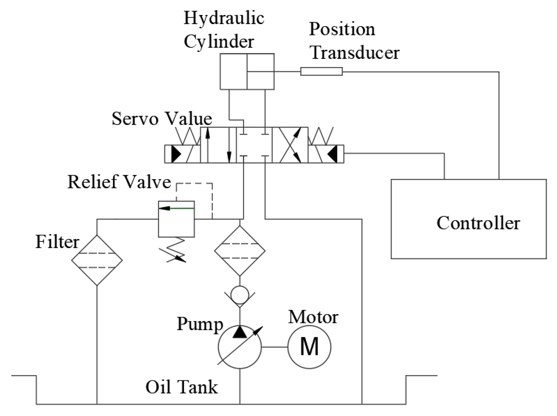
2.1. Introduction of Hydraulic Servo System

As shown in Figure 1, the system consists of a hydraulic pump, servo valve, position transducer, hydraulic cylinder, controller, etc. In each sampling time, the controller measures the tracking signal through the position transducer and produces the control signal to the servo valve, thereby driving the hydraulic cylinder.

2.2. Mathematical Model

The linearized flow equation is derived as follows based on the characteristics of the ideal servo valve [24].

$$q_L=K_q{x}_v-K_c{p}_L$$

(1)

where $q_L$ is the servo valve’s output flow, $K_q$ is the servo valve’s flow gain, $K_c$ is the flow pressure coefficient, $x_v$ is the displacement of the spool valve, and $p_L$ is the load pressure.

The servo amplifier and servo valve are equivalent to the proportional link, and the equations are given by [7,8]:

$$K_u=\frac{\mathrm{i}}{u}$$

(2)

$$K_{pv}=\frac{x_v}{\mathrm{i}}$$

(3)

where $K_u$ is the amplification factor of the servo amplifier; $K_{pv}$ is the gain of the servo valve; $\mathrm{i}$ is the input current of the servo amplifier; $u$ is the input voltage of the servo amplifier, and $x_v$ is the displacement of the servo spool valve.

According to Equations (2) and (3), the relation between the displacement of the servo valve spool and the control signal is as follows:

$$x_v=K_{pv}{K}_{u}u$$

(4)

According to Equation (4), the total flow $Q_L$ is:

$$Q_L=q_L=K_{pv}{K}_u{K}_{q}u-K_c{p}_L$$

(5)

According to the flow continuity equation [25], the flow continuity equation of the obtained asymmetrical hydraulic cylinder is:

$$q_L=A_1\frac{d{x}_p}{dt}+\frac{V_t}{2(1+n^2){\beta }_e}\frac{d{p}_L}{dt}+C_t{p}_L$$

(6)

where $A_1$ is the area of the hydraulic cylinder piston; $x_P$ is the displacement of the piston; $C_t$ is the external leakage coefficient of the hydraulic cylinder; $V_t$ is the total volume of the pipeline and the hydraulic cylinder; ${\beta }_e$ is the volumetric elastic modulus of the hydraulic cylinder; and $n$ is the ratio of the effective area of the rod cavity of the hydraulic cylinder to that of the rod-free cavity [8].

The force balance equation of the piston is as follows [26]:

$$A_1{p}_L=m_t\frac{d^2{x}_p}{d{t}^2}+B_p\frac{d{x}_p}{dt}+K_p{x}_p+F$$

(7)

where $m_t$ is the total mass of the piston and the load; $B_p$ is the viscous damping coefficient of the rod and load; $K_p$ is the elastic stiffness coefficient; and $F$ is the external load force acting on the hydraulic cylinder.

According to Equations (5)–(7), the dynamic model of the system is as follows [27]:

$$Ku=M_y{\stackrel{⃛}{x}}_p+B_y{\ddot{x}}_p+C_{{}_y}\dot{x}+D_y{x}_p+d_y$$

(8)

where $K=K_{pv}{K}_u{K}_q$, $M_y=\frac{V_t{m}_t}{2(1+n^2){\beta }_e{A}_1}$, $B_y=\frac{V_t{B}_p+2(1+n^2){\beta }_e{K}_{CE}{m}_t}{2(1+n^2){\beta }_e{A}_1}$, $C_y=\frac{A_1{}^2+K_p{V}_t}{2(1+n^2){\beta }_e{A}_1}$, $D_y=\frac{K_{CE}{K}_p}{A_1}$ and $d_y=\frac{V_t}{2(1+n^2)}\frac{\dot{F}}{A_1}+\frac{K_{CE}}{A_1}F$.

In the above equations, it assumes $x_1=x_p$, $x_2={\dot{x}}_p$, $x_3={\ddot{x}}_p$, where $x_1$, $x_2$, and $x_3$, respectively, represent the displacement, velocity, and acceleration of the piston. The system’s state space equation can be expressed as [28]:

$$\left\{\begin{array}{c}\dot{x}=Ax+Bu+D\\ y=Cx\end{array}\right.$$

(9)

where $x=\left[x_1,x_2,x_3\right]$, $A=\left[\begin{array}{ccc}0& 1& 0\\ 0& 0& 1\\ a_1& a_2& a_3\end{array}\right]$, $B=\left[\begin{array}{c}0\\ 0\\ G\end{array}\right]$, $C=\left[\begin{array}{ccc}1& 0& 0\end{array}\right]$, $D={\left[\begin{array}{ccc}0& 0& d\end{array}\right]}^T$, $a_1=-\frac{4{\beta }_e{K}_{CE}{K}_p}{m_t{V}_t}$, $a_2=-\frac{K_p}{m_t}-\frac{4{\beta }_e}{m_t{V}_t}\left(A_1{}^2+K_{CE}{B}_p\right)$, $a_3=-\frac{B_p}{m_t}-\frac{4{\beta }_e{K}_{CE}}{V_t}$, $G=\frac{4{\beta }_e{A}_1}{V_t{m}_t}(K_{pv}{K}_p{K}_q)$ and $d=-\frac{\dot{F}}{m_t}-\frac{4{\beta }_e{K}_{CE}}{m_t{V}_t}F$, where $u$ is the system input; $y$ is the system output, $d$ is the external disturbance. When the piston is moving in the positive direction, $K_q=Cw\sqrt{\frac{2\left(p_s-p_L\right)}{\rho \left(1+n^3\right)}}$, $K_{CE}=C_t-C_{d}wx\frac{\sqrt{\frac{2\left(p_s-p_L\right)}{\rho \left(1+n^3\right)}}}{2\left(p_s-p_L\right)}$; otherwise, $K_q=C_{d}w\sqrt{\frac{2\left(n{p}_s+p_L\right)}{\rho \left(1+n^3\right)}}$, $K_{CE}=C_t-C_{d}wx\frac{\sqrt{\frac{2\left(n{p}_s+p_L\right)}{\rho \left(1+n^3\right)}}}{2\left(n{p}_s+p_L\right)}$.

3. SAC-PID Control Strategy

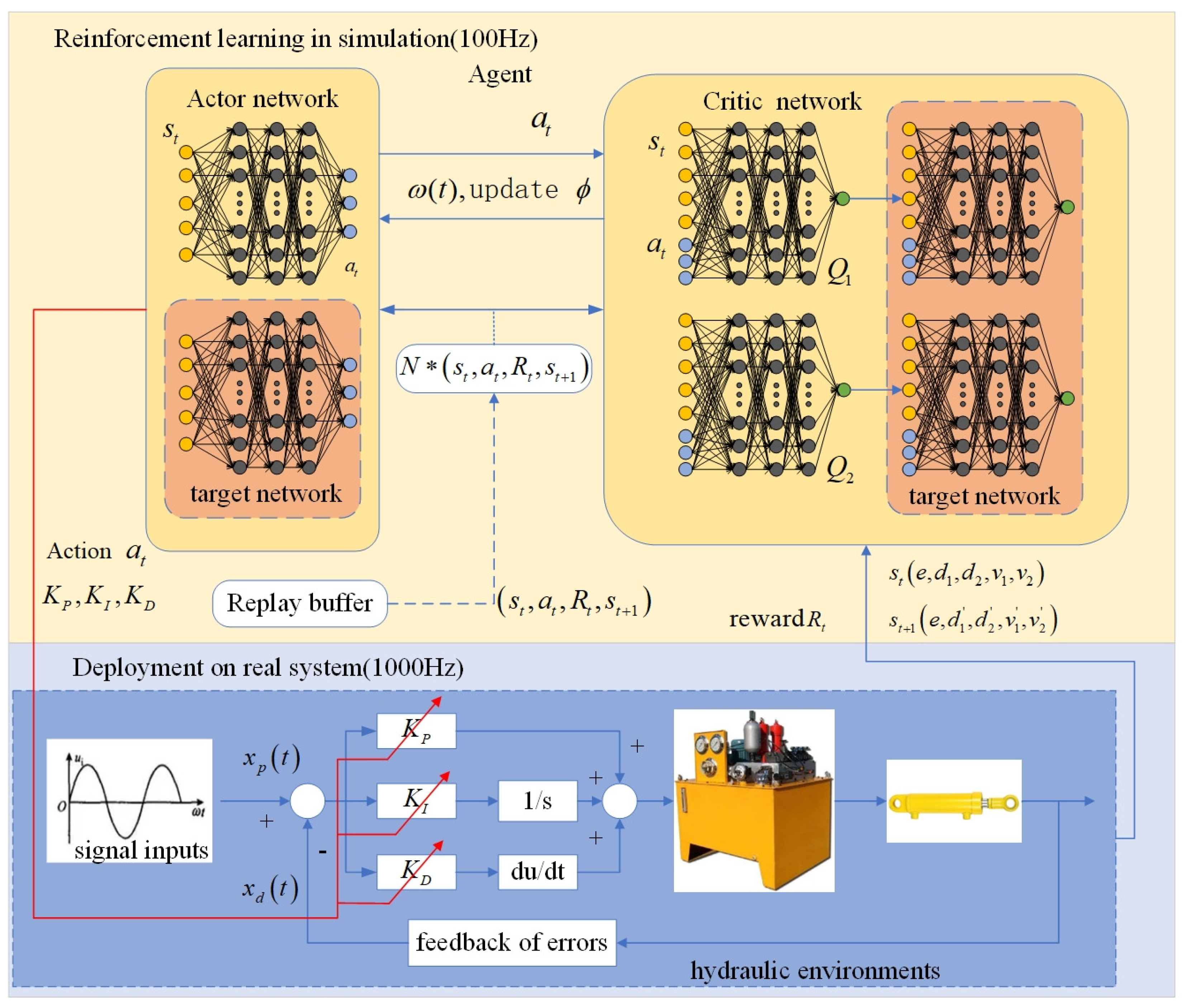
3.1. Overview of the Control Strategy

Compared to the DDPG algorithm, SAC algorithm employs a stochastic exploration strategy that has demonstrated superior performance in open benchmark tests and has been successfully applied to real-world control applications [29]. As shown in Figure 2, we propose a hierarchical controller with an upper controller based on the SAC algorithm and a lower controller based on the PID method. The upper controller continuously adjusts the lower controller’s parameters based on the system’s feedback and tracking error, enabling the lower controller, which runs at 10 times the frequency of the upper controller, to achieve more precise tracking performance, particularly in the presence of unknown disturbances and system uncertainties.

The critic and actor neural networks [30] in the upper controller comprise an input layer, three hidden layers, and an output layer. The rectified linear unit (ReLU) function is adopted as the activation function in the hidden layers, which maps the input to the output signal. The critic network takes both the states $s_t$ and actions $a_t$ as input, while the action network takes only the states $s_t$ as input.

3.2. Design of the Upper Controller

The long-term reward $G_t$ obtained by an agent under a given action strategy can be expressed as Equation (10):

$$G_t=r_t+\gamma r_{t+1}+{\gamma }^2{r}_{t+2}+\dots ={\displaystyle \sum _{i=0}{\gamma }^i{r}_{i+1}}$$

(10)

where $\gamma$ is the discount factor and $r_t$ is the extrinsic reward.

This method employs a maximum entropy objective to facilitate the learning of policies for complex tasks:

$$J\left(\pi \right)={\displaystyle \sum _{t=0}^{T}E\left(s_t,a_t\right)}~{\rho }_{\pi }\left[r\left(s_t,a_t\right)+\alpha H\left(\pi \left(\cdot |s_t\right)\right)\right]$$

(11)

where $\alpha$ is a temperature coefficient. The action state value function $Q\left(s_t,a_t\right)$ in maximum entropy objective can be formulated as Equation (12) [31]:

$$Q\left(s_t,a_t\right)=r\left(s_t,a_t\right)+\gamma E_{S_{t+1}~p}\left[V\left(s_{t+1}\right)\right]$$

(12)

where

$$V\left(s_t\right)=E_{a_t~\pi }\left[Q\left(s_t,a_t\right)-\alpha \log \pi \left(a_t|s_t\right)\right]$$

(13)

The updated critic networks to minimize the loss function can be formulated as Equation (14):

$$J_Q\left(\theta \right)=E_{\left(s_t,a_t\right)~D}\left[\frac{1}{2}{\left(Q_{\theta }\left(s_t,a_t\right)-\widehat{Q}\left(s_t,a_t\right)\right)}^2\right]$$

(14)

With

$$\widehat{Q}\left(s_t,a_t\right)=r\left(s_t,a_t\right)+\gamma E_{s_{t-1}~p}\left[V_{\overline{\psi }}\left(s_{t+1}\right)\right]$$

(15)

The updated of policy ${\pi }_{\varphi }$ trained by actor networks can be expressed as Equation (16):

$$J_{\pi }\left(\varphi \right)=E_{s_t\sim D,{\in }_t\sim {\pi }_{\varphi }}\left[\log {\pi }_{\varphi }\left(f\left({\in }_t;s_t\right)|s_t\right)-Q_{\theta }\left(s_t,f\left({\in }_t;s_t\right)\right)\right]$$

(16)

where ${\in }_t$ is the input noise vector, which is sampled from spherical Gaussian [29].

The reward function is crucial in the upper controller as it determines the controller’s behavior and guides the learning process toward achieving the desired goals. The reward function must consider several factors in the upper controller to ensure effective tracking performance. Firstly, the function should prioritize minimizing the tracking error when following input signals. Secondly, it should encourage reducing the tracking error by comparing the current error $e_{x_t}$ and the previous error $e_{x_{t-1}}$. Thirdly, the function should discourage excessive acceleration to avoid oscillations. To incorporate these considerations, we design the reward function as follows:

$$\left\{\begin{array}{l}r\left(s\right)=r_1+r_2+r_3\hfill \\ r_1=k_1\left|e_x\right|\hfill \\ r_2=\left\{\begin{array}{c}\begin{array}{cc}{k}_2& \left|e_{x_t}\right|>\left|e_{x_{t-1}}\right|\end{array}\\ \begin{array}{cc}{k}_3& \left|e_{x_t}\right|<\left|e_{x_{t-1}}\right|\end{array}\end{array}\right.\hfill \\ r_3=k_4\left|a\right|\hfill \end{array}\right.$$

(17)

where $a$ represents the current acceleration and $k_1, k_2, k_3, k_4$ are negative gain coefficients.

3.3. Algorithm Statement

The proposed control algorithm comprises three phases: initialization, interaction, and optimization. In the initialization phase, the system loads the parameter settings and initializes an empty replay buffer to store the transition tuples.

During the interaction phase, as depicted in Algorithm 1, the agent observes the current state $s_t$, selects an action by sampling from the current actor network according to $s_t$, and receives a reward $r_t$ after executing the action. The transition tuple $(s_t,a_t,r_t,s_{t+1})$ is stored in the replay buffer R after transitioning to the next state $s_{t+1}$.

Algorithm 1: Pseudocode of the SAC-PID control strategy.

Initialize the relevant parameters of the policy network, replay buffer size  for t = 1, 2, … do  $e(t)=x_p(t)-x_d(t)$  $u(t)=K_{P}e(t)+K_I{\displaystyle \sum _{n=0}^{t}e(n)+K_D\left(e\left(t\right)-e\left(t-1\right)\right)}$   if t = 10, 20, … do     for episode = 1, 2, …, E do      Receive initial state $s_1$       for step = 1, 2, …, T1 do        Select actions $a_t$ based on the current state $s_t$        Compute the control signals $u(t)$ according to the action $a_t$        Apply control signals $u(t)$ and observe the next state $s_{t+1}$        Compute the current reward $r_t$        Store following $transition (s_t,a_t,r_t,s_{t+1})$ into replay buffer R           if it is time to update then               Update Q network parameters:$Q_i\leftarrow Q_i-{\lambda }_Q{\widehat{\nabla }}_{Q_i}J\left(Q_i\right)fori\in \left\{1,2\right\}$            Update critic network parameters:$\pi \leftarrow \pi -{\lambda }_{\pi }{\widehat{\nabla }}_{\pi }J\left(\pi \right)$            Update entropy parameters:$\alpha \leftarrow \alpha -\lambda {\widehat{\nabla }}_{\pi }J\left(\alpha \right)$            Updating of target network parameters online           End if        End for     End for    End if  End for

In the optimization phase, the policy $J\left(Q_i\right)$ is optimized using two Q functions during each gradient step. The actor network parameters are updated using the minimum Q-functions for policy gradient in Equation (12). The target network loss function is updated according to Equation (14), and the entropy parameters are updated automatically. Finally, the target network parameters are updated online using Equation (16) where ${\lambda }_Q$ denotes the learning rate and ${\lambda }_{\pi }$ is the target smoothing coefficient.

4. Simulation Environments

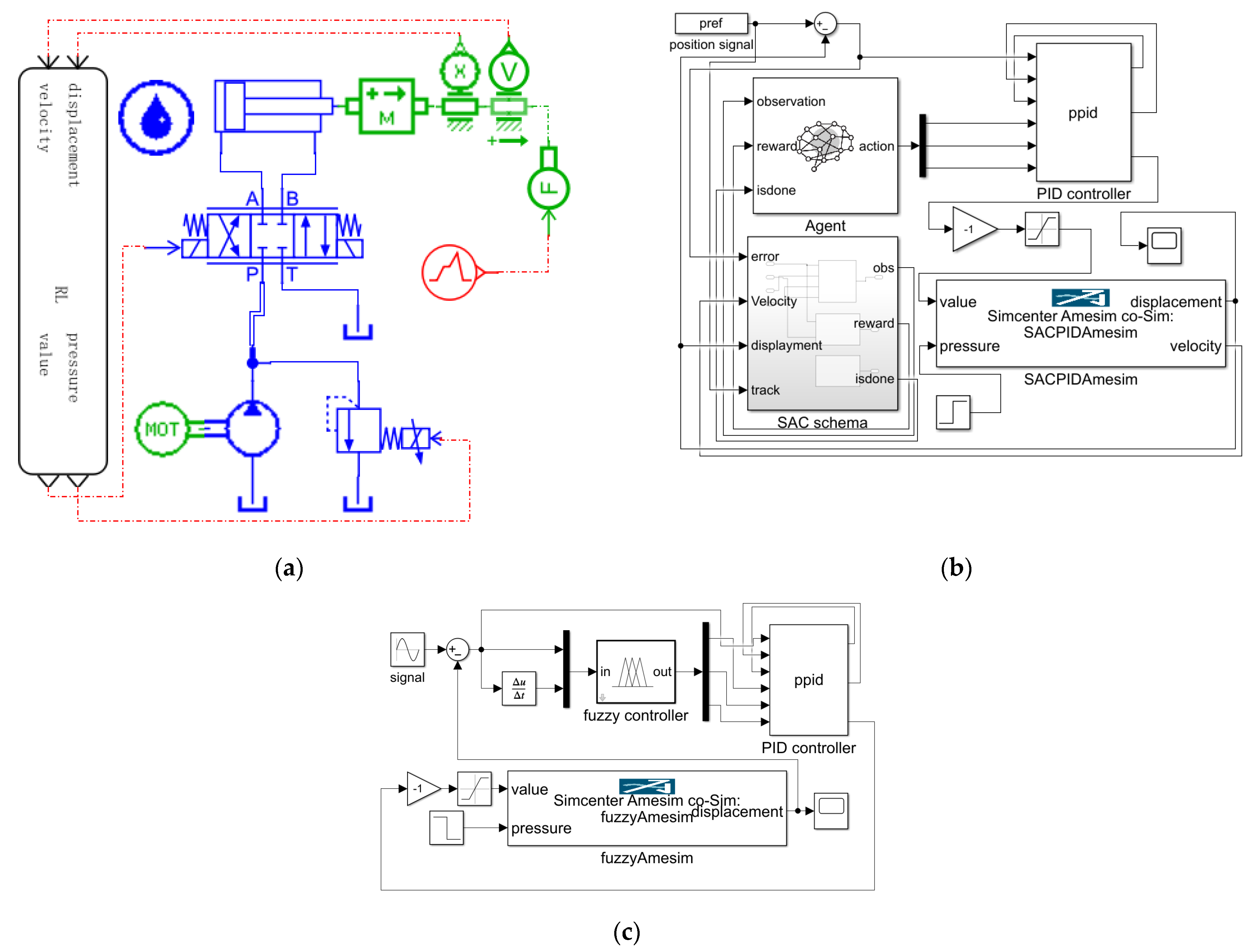
4.1. Simulation Setup

Fuzzy PID control offers the advantage of adaptivity as it can dynamically adjust the controller’s parameters based on fuzzy rules. Therefore, we chose the fuzzy PID control strategy as the baseline to compare with the SAC-PID control strategy. Figure 3 depicts the co-simulation model of the proposed SAC-PID control strategy and fuzzy PID control strategy, which were implemented in AMESim and Matlab software. The main parameters [27] used in the model are shown in

Table 1. Simulation parameters.

Parameter	Value	Parameter	Value
Pump displacement	$5e^{-6} {\mathrm{m}}^3/\mathrm{rev}$	Actuator stroke	$0.2 \mathrm{m}$
Motor speed	$1420 \mathrm{rev}/\min$	Rod diameter	$0.05 \mathrm{m}$
Servo valve’s natural frequency	$65 \mathrm{Hz}$	Piston diameter	$0.1 \mathrm{m}$
Servo valve’s input signal	$\pm 10 \mathrm{V}$	Load mass	$100 \mathrm{Kg}$
Servo valve’s max flow	$4 \mathrm{L}/\min$	Relief valve’s opening pressure	$15 \mathrm{MPa}$

, and the co-simulation step is 1 ms. As shown in Figure 3a, the AMESim hydraulic system model consists of a quantitative pump model, a single-acting hydraulic cylinder model with load, a servo motor model, and two piston rod displacement and velocity measurement sensors. Figure 3b shows that the Simulink model consists of a PID controller, a co-simulation interface, and the SAC strategy model. As shown in Figure 3c, the inputs of the fuzzy controller are the tracking error and the derivative of the tracking error; the output of that is the input parameters of the PID controller.

Table 2. Training hyperparameters setting.

Parameter	Value
Nonlinearity	ReLU
Optimizer	Adam
Learning rate (${\lambda }_Q$ and ${\lambda }_{\pi }$)	0.001
Discount rate $\left(\gamma \right)$	0.99
Size of the replay buffer	$1\times {10}^6$
Numbers of the hidden layers (all networks)	128

presents the hyperparameters used in the SAC-PID control strategy [23,31]. The figures below illustrate the desired trajectory signals, SAC-PID, PID, and fuzzy PID control response and tracking error $e(t)$ curves. Specifically, SPID represents the response and tracking error of SAC-PID, while PID and FPID denote the response and tracking errors of PID control and fuzzy PID control, respectively. Tracking error $e(t)=x_p(t)-x_d(t)$, where $x_p(t)$ is desired trajectory signals, and $x_d(t)$ is tracking response signals.

The fuzzy PID control serves as a comparison experiment with SPID control in this study. The fuzzy rules utilized in the fuzzy PID control are presented in

Table 3. Fuzzy rules for FPID control.

$\mathit{d}\mathit{e}/\mathit{e}$	NB	NM	NS	Z	PS	PM	PB
NB	NB	NB	NB	NM	NM	NS	Z
NM	NB	NB	NM	NS	NS	Z	PS
NS	NB	NM	NS	NS	Z	PS	PM
Z	NM	NS	NS	Z	PS	PS	PM
PS	NM	NS	Z	PS	PS	PM	PB
PM	NS	Z	PS	PS	PM	PB	PB
PB	Z	PS	PM	PM	PB	PB	PB

[9], and they are $e$ (tracking error), $de$ (derivative of tracking error), NB (negative big), NM (negative middle), NS (negative small), ZO (zero), PS (positive small), PM (positive middle), and PB (positive big). The values of $e$, $de$, $K_P$, $K_I$, and $K_D$ are constrained within the range of $e\in \left(-1,1\right)$, $de\in \left(-1,1\right)$, $K_P\in \left(60,120\right)$, $K_I\in \left(1,20\right)$, and $K_D\in \left(0.1,0.6\right)$, respectively.

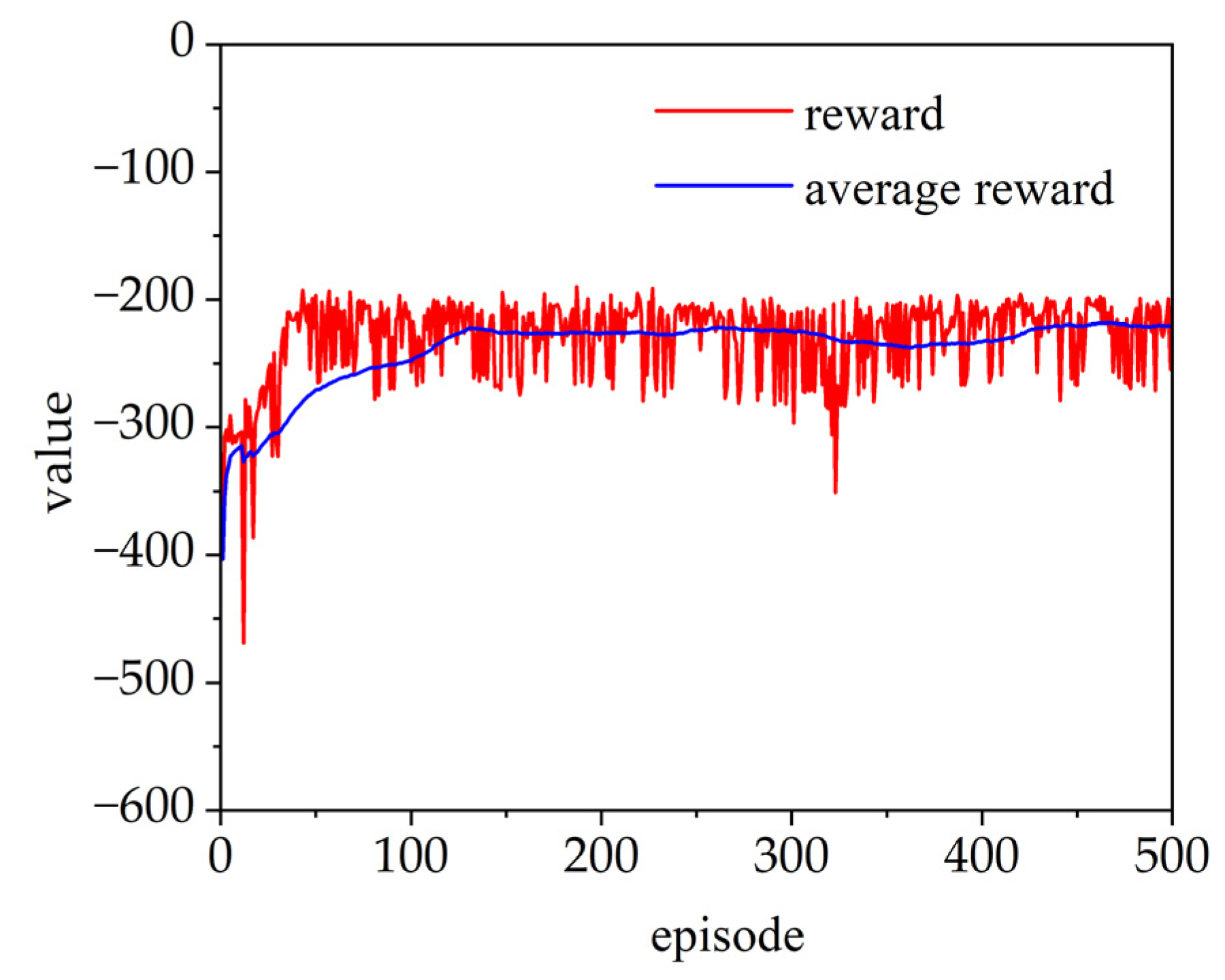
4.2. Training Samples Setup

The whole simulation process is divided into two phases: the training phase and the testing phase. For each training episode (lasting 4 s), we randomly selected tracking signals in

Table 4. Design of training samples.

Sample Types		Training Samples
Random signals	Ramp	$y=\left\{\begin{array}{cc}kt& t\le t_0\\ k{t}_0& t>t_0\end{array}\right.$$k\in \left[1,8\right],k\in N,t_0\in \left[1,3\right]$
	Sinusoidal	$y=a\sin (b\pi t)$ $a\in \left[0.5,8\right],b\in \left[0.2,2\right]$
Signals with disturbance	Pressure drop	$y=2\sin (0.5\pi t)$ $P=\left\{\begin{array}{cc}14& t\le t_0\\ Z& t>t_0\end{array}\right.$$Z\in \left[4,10\right],t_0\in \left[1,3\right]$
	Transient force	$y=2\sin (0.5\pi t)$ $F=\left\{\begin{array}{cc}0& t\notin \left(t_0,t_0+0.02\right)\\ Z& t\in \left(t_0,t_0+0.02\right)\end{array}\right.$$Z\in \left[5,15\right],t_0\in \left[1,3.5\right]$

and randomly assigned values to parameters such as $k$, $t_0$, $a$, and $b$ in the given range. Table 4 displays the signals trained during a single training session for the SAC-PID control strategy. The ramp signals are denoted as $y=\left\{\begin{array}{cc}kt& t\le t_0\\ k{t}_0& t>t_0\end{array}\right.$, with $k$ taking integer values from one to eight and reaching a stable segment at a randomly selected time between one to three seconds. The sinusoidal signal samples are denoted as $y=a\sin \left(b\pi *t\right)$, with $a$ being a random number between 0.5 to 8 and $b$ being a random number between 0.2 to 2.

To enhance the tracking performance of the SAC-PID control strategy under varying system parameters and external disturbances, we devised two types of training samples with interference. The first type involves a sudden drop in hydraulic system pressure from 14 Mpa to a random value between 4 Mpa to 10 Mpa. The second type involves a random transient force of 5 KN to 15 KN randomly appearing for 0.02 s between 1 and 3.5 s.

5. Simulation Results

5.1. The Tracking Response of Random Signals Input

Figure 4 shows the training process of the SAC-PID control strategy using random tracking trajectories, with the average reward value stabilizing after 100 episodes. The average reward curve demonstrates a consistent upward trend, signifying a stable training process.

In the testing phase we use the trained model. Specifically, the parameters of the trained model cannot be changed, and the upper-level controller does not explore in the testing process. During the test, the PID control parameters are set to $K_P=83,K_I=12,K_D=0.2$ when tracking random ramp signals $y=\left\{\begin{array}{cc}2t& t\le 3\\ 6& t>3\end{array}\right.$(S1.1), $y=\left\{\begin{array}{cc}4t& t\le 3\\ 12& t>3\end{array}\right.$(S1.2), $y=\left\{\begin{array}{cc}6t& t\le 3\\ 18& t>3\end{array}\right.$(S1.3), and $y=\left\{\begin{array}{cc}8t& t\le 3\\ 24& t>3\end{array}\right.$(S1.4), respectively.

The performance of SAC-PID in tracking S1.2 was evaluated, and the results are illustrated in Figure 5. In the simulation, the PID control resulted in significant hysteresis with a maximum overshoot of 0.022 mm and a relatively slow convergency. In contrast, the fuzzy PID control produces a minor overshoot of approximately 0.071 mm and $6e^{-4}$ mm oscillation in steady-state. Otherwise, the maximum overshoot of SAC-PID control is approximately 0.046 mm, which is much smaller than that of fuzzy PID and PID control. The corresponding integral of time and absolute error (ITAE) values when tracking S1.1–S1.4 using the three control methods are presented in

Table 5. ITAE values for PID, fuzzy PID, and SAC-PID when tracking different ramp signals.

Ramp Signals/ Control Strategies	PID	Fuzzy PID	SAC-PID
S1.1	116.82	6.81	3.94
S1.2	255.64	10.22	7.57
S1.3	336.23	14.82	11.67
S1.4	446.84	28.63	28.34

, which indicates that the control performance of SAC-PID control is significantly higher than that of fuzzy and PID control.

During the test, the PID control parameters are set to $K_P=83,K_I=12,K_D=0.2$ when tracking random sinusoidal signals $y=\sin \left(5\pi *t/4\right)$ (S2.1), $y=2\sin \left(\pi *t\right)$ (S2.2), $y=3\sin \left(3\pi *t/4\right)$ (S2.3), and $y=4\sin \left(\pi *t/2\right)$ (S2.4), respectively.

The simulation responses and tracking errors of the sinusoidal signal input (S2.2) are depicted in Figure 6, indicating that the tracking error of the SAC-PID control is reduced by 95.1% compared to the PID control and 64.7% compared to the fuzzy PID control. The corresponding ITAE values when tracking S2.1–S2.4 are presented in

Table 6. ITAE values for PID, fuzzy PID, and SAC-PID when tracking different sinusoidal signals.

Sinusoidal Signals/ Control Strategies	PID	Fuzzy PID	SAC-PID
S 2.1	268.71	54.77	16.97
S 2.2	427.51	71.14	22.53
S 2.3	482.68	62.55	21.79
S 2.4	437.08	36.90	12.98

, indicating that the SPID control strategy has the best control performance when tracking random sinusoidal signals.

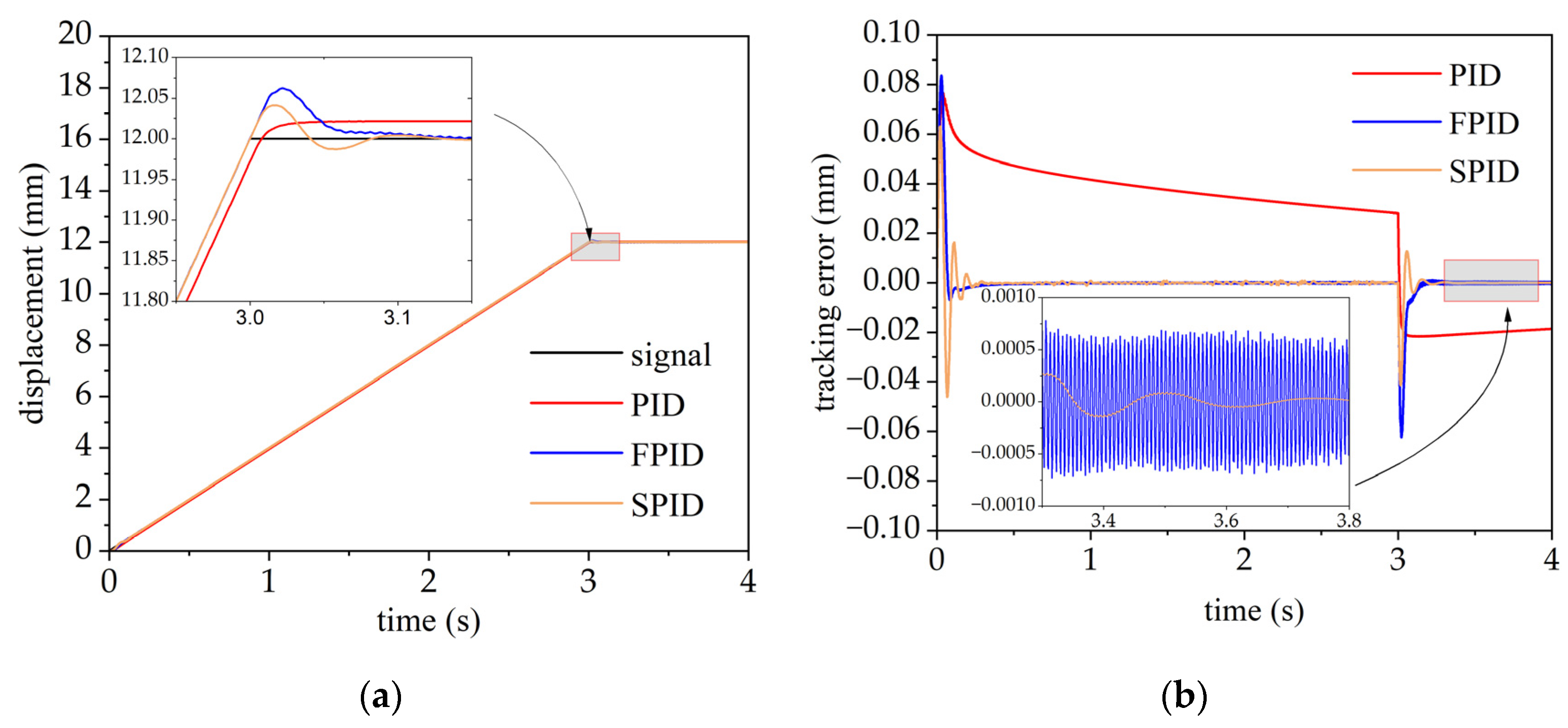
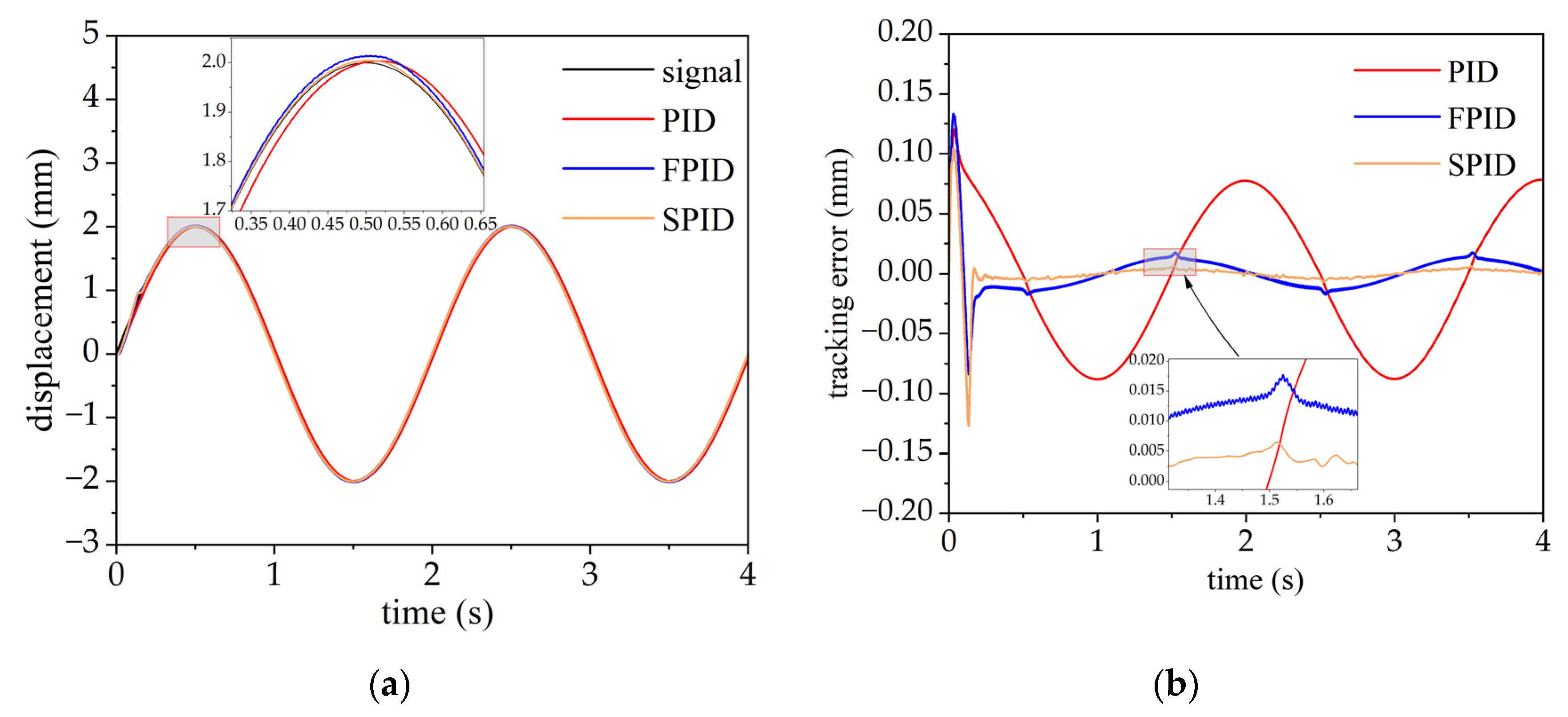
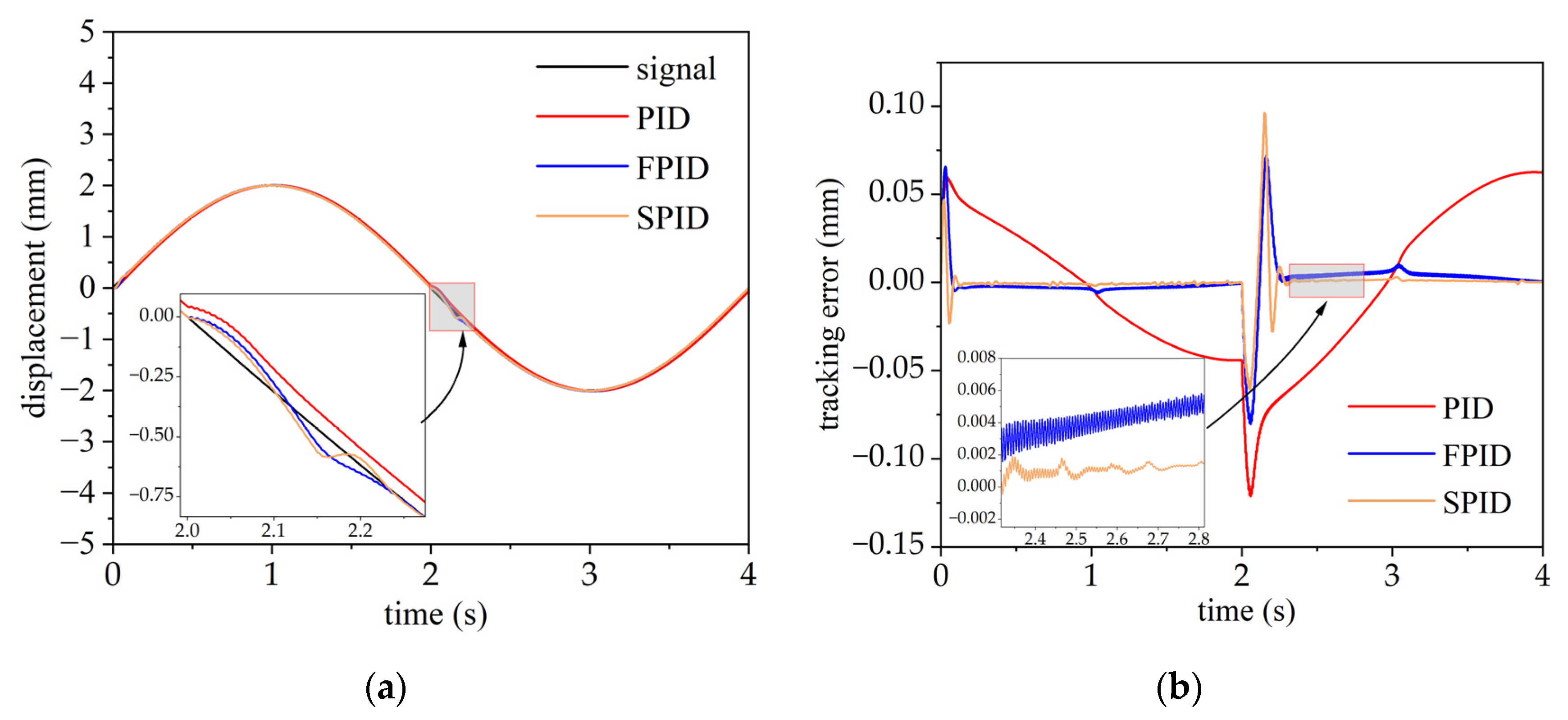
5.2. The Tracking Response of Sinusoidal Signals Input with Sudden Pressure Drop

During the test, the PID control parameters are set to $K_P=83,K_I=12,K_D=0.2$ when tracking sinusoidal signals $y=2\sin (0.5\pi t)$ with varying system parameters $P=\left\{\begin{array}{cc}14& t\le 1\\ 10& t>1\end{array}\right.$ (W1.1), $P=\left\{\begin{array}{cc}14& t\le 1.5\\ 8& t>1.5\end{array}\right.$ (W1.2), $P=\left\{\begin{array}{cc}14& t\le 2\\ 6& t>2\end{array}\right.$ (W1.3), and $P=\left\{\begin{array}{cc}14& t\le 2.5\\ 4& t>2.5\end{array}\right.$ (W1.4), respectively, where the unit of P is MPa. The training process using sinusoidal signals with sudden system pressure drop is shown in Figure 7.

Figure 8 presents the simulation responses and response errors of the sinusoidal signal input with sudden pressure drop (W1.3) for the three control strategies. The simulation lasts 4 s, and the system pressure drops suddenly from 14 MPa to 6 MPa at 2.0 s. The SAC-PID control achieves the best anti-disturbance performance in the presence of a system pressure drop. In contrast, the PID control produces the largest overshoot while the fuzzy PID control produces severe oscillations, indicating that the varying hydraulic servo system parameters have a significant impact on the control performance of the system and that the SAC-PID control strategy can effectively suppress the adverse effects of varying system parameters.

Table 7. ITAE values for PID, fuzzy PID, and SAC-PID when tracking sinusoidal signals with different pressure drops.

Pressure Drop/ Control Strategies	PID	Fuzzy PID	SAC-PID
W 1.1	257.29	22.31	7.24
W 1.2	285.92	27.45	11.17
W 1.3	329.63	48.10	26.19
W 1.4	427.57	169.36	142.65

demonstrates that the SAC-PID control scheme outperformed the PID control and fuzzy PID control, reducing tracking errors of at least 66.7% and 15.8%, respectively.

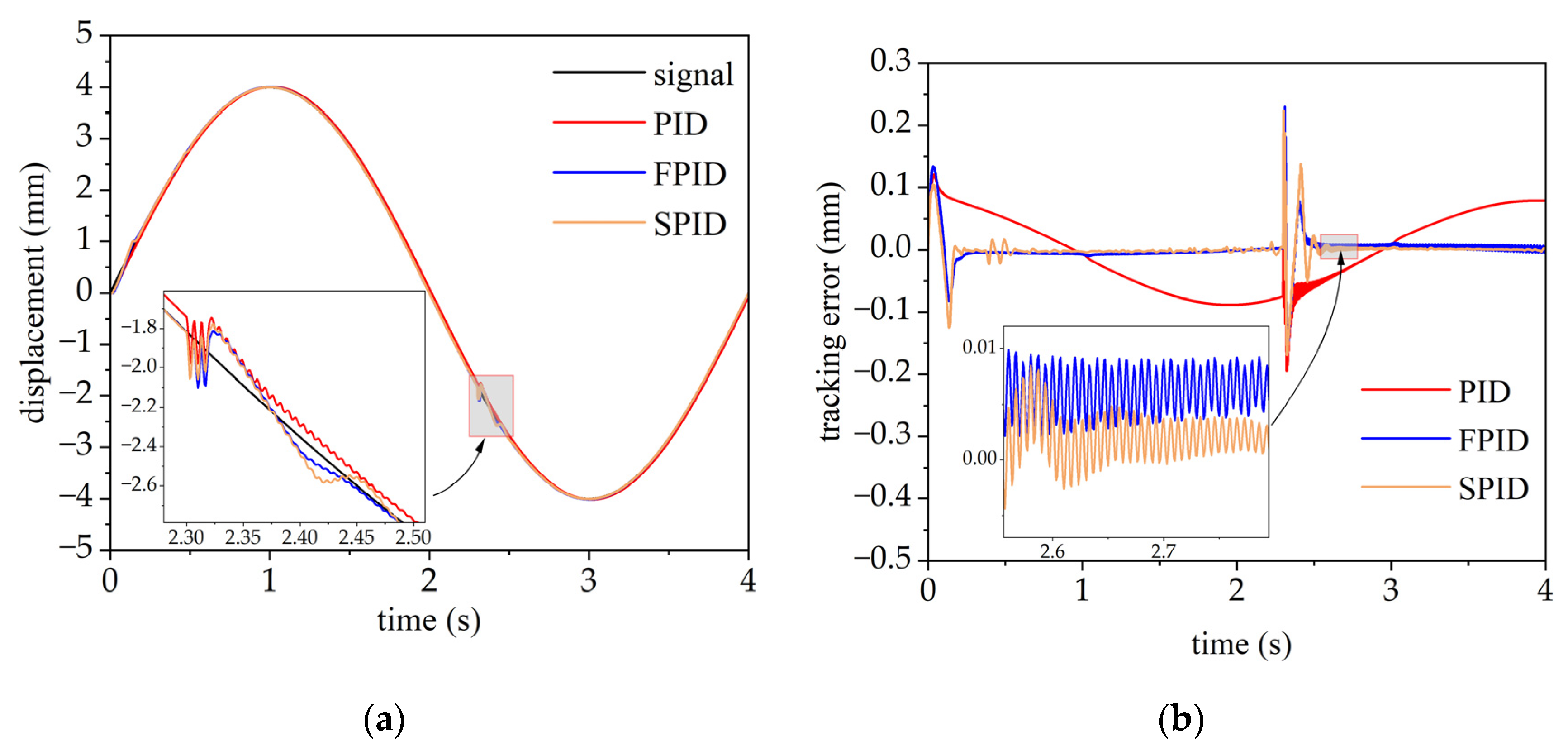
5.3. The Response of Sinusoidal Signals Input with External Disturbance Force

During the test, the PID control parameters are set to $K_P=83,K_I=12,K_D=0.2$ when tracking the sinusoidal signal $y=4\sin (0.5\pi t)$ with external disturbance transient force $F=\left\{\begin{array}{cc}0& 1.3\le t\le 1.32\\ 5& t<1.3 or t>1.32\end{array}\right.$ (W2.1), $F=\left\{\begin{array}{cc}0& 2.3\le t\le 2.32\\ 10& t<2.3 or t>2.32\end{array}\right.$ (W2.2), and $F=\left\{\begin{array}{cc}0& 3.3\le t\le 3.32\\ 15& t<3.3 or t>3.32\end{array}\right.$ (W2.3), respectively, where the unit of $F$ is $\mathrm{kN}$.

Figure 9 presents the responses and response errors of the sinusoidal signal input with external transient force (W2.2). The simulation lasts 4 s and a disturbance force (amplitude 10 kN, starting at 2.3 s and stopping at 2.32 s) is added to the load. The graph shows that all three control strategies lead to significant chattering in the response when disturbance forces are present in the hydraulic servo system. However, in contrast to PID and fuzzy PID control, the SAC-PID control strategy results in minimal response oscillations and can rapidly damp oscillations.

Table 8. ITAE values for PID, fuzzy PID, and SAC-PID when tracking sinusoidal signals with external disturbance force.

Transient Force/ Control Strategies	PID	Fuzzy PID	SAC-PID
W 2.1	437.82	44.75	22.99
W 2.2	443.19	63.21	46.11
W 2.3	447.73	80.08	57.79

demonstrates that when tracking sinusoidal signals with external disturbance force, the SAC-PID control strategy outperformed the PID control and fuzzy PID control, reducing tracking errors by at least 87.1% and 27.1%, respectively.

When tracking the sinusoidal signal with disturbance force W2.2, the comparison of the PID parameters of fuzzy PID and SAC-PID are shown in Figure 9, indicating that the PID parameters of the two control strategies are adaptive updating effectively improve the performance of the control system.

Figure 9 compares the adaptive updated PID parameters between fuzzy PID and SAC-PID control when tracking the sinusoidal signal with disturbance force W2.2. FKP, FKI, and FKD represent the PID parameters $K_P$, $K_I$, and $K_D$ of fuzzy PID control, respectively, while SKP, SKI, and SKD represent the PID parameters $K_P$, $K_I$, and $K_D$ of SAC-PID control, respectively. The results show that the PID parameters in both control strategies can be automatically tuned according to the tracking signal, which enhances the control performance of the hydraulic servo system.

Figure 10a illustrates that when the hydraulic cylinder rod extends, the $K_P$ in SAC-PID control significantly increases compared to when the hydraulic cylinder rod retracts (from one second to three seconds). This indicates that compared with fuzzy PID control, SAC-PID control can effectively learn the critical characteristics of the hydraulic servo system, leading to proactive adjustment of the $K_P$ and reducing the performance difference in tracking when the rod extends and retracts. Figure 10b,c demonstrate that when disturbance force occurs (start at 2.3 s), the $K_I$ and $K_D$ in SAC-PID control significantly decrease compared to fuzzy PID control. This results in SAC-PID control exhibiting better anti-disturbance capability.

6. Conclusions

This study proposes a novel SAC-PID control strategy to improve the control performance of hydraulic servo systems with PID control, especially in the presence of nonlinearity and uncertainty. The SAC-PID control strategy comprises an upper-level controller based on the SAC algorithm and a lower-level controller based on the PID control method. The upper-level controller learns the hydraulic servo system’s hydraulic and disturbance characteristics, enabling dynamic PID parameter adjustment in the lower-level controller. The proposed control strategy can effectively suppress the adverse effects of various uncertainties on the hydraulic servo system.

Simulation experiments were conducted to track random signals, sinusoidal signals with sudden system pressure drops, and sinusoidal signals with external disturbance forces using the SAC-PID, fuzzy PID, and PID control schemes, respectively. The results indicate that when tracking random signals, the SAC-PID control strategy exhibits superior performance compared to the PID and fuzzy PID control strategies, achieving an average track error reduction of 95.6% and 44.7%, respectively. Similarly, when tracking sinusoidal signals with internal and external disturbance, the SAC-PID control strategy outperforms the PID and fuzzy PID control strategies, with an average track error reduction of 89.1% and 41.7%, respectively.

Analysis of PID parameter variation during fuzzy PID and SAC-PID simulation experiments showed that the proposed SAC-PID control strategy efficiently optimizes PID parameters based on tracking errors and learned system characteristics, resulting in improved tracking accuracies in hydraulic servo systems. This approach has significant potential for enhancing hydraulic servo systems’ control accuracy and robustness in various practical applications.

References

1. Huayong, Y.; Hu, S.; Guofang, G.; Guoliang, H. Electro-hydraulic proportional control of thrust system for shield tunneling machine. Autom. Constr. 2009, 18, 950–956. [Google Scholar] [CrossRef]
2. Nguyen, M.T.; Dang, T.D.; Ahn, K.K. Application of Electro-Hydraulic Actuator System to Control Continuously Variable Transmission in Wind Energy Converter. Energies 2019, 12, 2499. [Google Scholar] [CrossRef]
3. Sivčev, S.; Rossi, M.; Coleman, J.; Dooly, G.; Omerdić, E.; Toal, D. Fully automatic visual servoing control for work-class marine intervention ROVs. Control Eng. Pract. 2018, 74, 153–167. [Google Scholar] [CrossRef]
4. Kim, S.; Park, J.; Kang, S.; Kim, P.Y.; Kim, H.J. A Robust Control Approach for Hydraulic Excavators Using μ-synthesis. Int. J. Control Autom. Syst. 2018, 16, 1615–1628. [Google Scholar]
5. Wang, Y.; Zhang, J.; Zhang, H.; Xie, X. Adaptive Fuzzy Output-Constrained Control for Nonlinear Stochastic Systems With Input Delay and Unknown Control Coefficients. IEEE Trans. Cybern. 2021, 51, 5279–5290. [Google Scholar] [CrossRef]
6. Chen, Z.; Yuan, X.; Ji, B.; Wang, P.; Tian, H. Design of a fractional order PID controller for hydraulic turbine regulating system using chaotic non-dominated sorting genetic algorithm II. Energy Convers. Manag. 2014, 84, 390–404. [Google Scholar] [CrossRef]
7. Fan, Y.; Shao, J.; Sun, G. Optimized PID Controller Based on Beetle Antennae Search Algorithm for Electro-Hydraulic Position Servo Control System. Sensors 2019, 19, 2727. [Google Scholar] [CrossRef]
8. Wang, L.; Zhao, D.; Liu, F.; Liu, Q.; Zhang, Z. Active Disturbance Rejection Position Synchronous Control of Dual-Hydraulic Actuators with Unknown Dead-Zones. Sensors 2020, 20, 6124. [Google Scholar] [CrossRef]
9. Çetin, Ş.; Akkaya, A.V. Simulation and hybrid fuzzy-PID control for positioning of a hydraulic system. Nonlinear Dyn. 2010, 61, 465–476. [Google Scholar] [CrossRef]
10. Jin, X.; Chen, K.; Zhao, Y.; Ji, J.; Jing, P. Simulation of hydraulic transplanting robot control system based on fuzzy PID controller. Measurement 2020, 164, 108023. [Google Scholar] [CrossRef]
11. Truong, D.Q.; Ahn, K.K. Force control for hydraulic load simulator using self-tuning grey predictor—Fuzzy PID. Mechatronics 2009, 19, 233–246. [Google Scholar] [CrossRef]
12. Shahid, A.A.; Piga, D.; Braghin, F.; Roveda, L. Continuous control actions learning and adaptation for robotic manipulation through reinforcement learning. Auton. Robot. 2022, 46, 483–498. [Google Scholar] [CrossRef]
13. Coronato, A.; Naeem, M.; De Pietro, G.; Paragliola, G. Reinforcement learning for intelligent healthcare applications: A survey. Artif. Intell. Med. 2020, 109, 101964. [Google Scholar] [CrossRef] [PubMed]
14. Han, M.; May, R.; Zhang, X.; Wang, X.; Pan, S.; Yan, D.; Jin, Y.; Xu, L. A review of reinforcement learning methodologies for controlling occupant comfort in buildings. Sustain. Cities Soc. 2019, 51, 101748. [Google Scholar] [CrossRef]
15. Song, Z.; Yang, J.; Mei, X.; Tao, T.; Xu, M. Deep reinforcement learning for permanent magnet synchronous motor speed control systems. Neural Comput. Appl. 2020, 33, 5409–5418. [Google Scholar] [CrossRef]
16. Naughton, N.; Sun, J.; Tekinalp, A.; Parthasarathy, T.; Chowdhary, G.; Gazzola, M. Elastica: A Compliant Mechanics Environment for Soft Robotic Control. IEEE Robot. Autom. Lett. 2021, 6, 3389–3396. [Google Scholar] [CrossRef]
17. Nascimento, T.P.; Saska, M. Position and attitude control of multi-rotor aerial vehicles: A survey. Annu. Rev. Control 2019, 48, 129–146. [Google Scholar] [CrossRef]
18. Yuan, X.; Wang, Y.; Zhang, R.; Gao, Q.; Zhou, Z.; Zhou, R.; Yin, F. Reinforcement Learning Control of Hydraulic Servo System Based on TD3 Algorithm. Machines 2022, 10, 1224. [Google Scholar] [CrossRef]
19. Wu, T.; Zhao, H.; Gao, B.; Meng, F. Energy-Saving for a Velocity Control System of a Pipe Isolation Tool Based on a Reinforcement Learning Method. Int. J. Precis. Eng. Manuf. Green Technol. 2021, 9, 225–240. [Google Scholar] [CrossRef]
20. Egli, P.; Hutter, M. A General Approach for the Automation of Hydraulic Excavator Arms Using Reinforcement Learning. IEEE Robot. Autom. Lett. 2022, 7, 5679–5686. [Google Scholar] [CrossRef]
21. Carlucho, I.; De Paula, M.; Villar, S.A.; Acosta, G.G. Incremental Q -learning strategy for adaptive PID control of mobile robots. Expert Syst. Appl. 2017, 80, 183–199. [Google Scholar] [CrossRef]
22. Yang, J.; Peng, W.; Sun, C. A Learning Control Method of Automated Vehicle Platoon at Straight Path with DDPG-Based PID. Electronics 2021, 10, 2580. [Google Scholar] [CrossRef]
23. Yu, X.; Fan, Y.; Xu, S.; Ou, L. A self-adaptive SAC-PID control approach based on reinforcement learning for mobile robots. Int. J. Robust Nonlinear Control 2021, 32, 9625–9643. [Google Scholar] [CrossRef]
24. Zhuang, H.; Sun, Q.; Chen, Z. Sliding mode control for electro-hydraulic proportional directional valve-controlled position tracking system based on an extended state observer. Asian J. Control 2020, 23, 1855–1869. [Google Scholar] [CrossRef]
25. He, D.; Wang, T.; Wang, J.; Ren, Z.; Gao, X. Research on the position–pressure cooperative control strategy for full-hydraulic leveler. Adv. Mech. Eng. 2018, 10, 1–14. [Google Scholar] [CrossRef]
26. Guo, W.; Zhao, Y.; Li, R.; Ding, H.; Zhang, J. Active Disturbance Rejection Control of Valve-Controlled Cylinder Servo Systems Based on MATLAB-AMESim Cosimulation. Complexity 2020, 2020, 9163675. [Google Scholar] [CrossRef]
27. Su, S.; Xue, T.; Chen, Y.; Yang, H. Harmonic control of a dual-valve hydraulic servo system with dynamically allocated flows. Asian J. Control 2022, 25, 1939–1956. [Google Scholar] [CrossRef]
28. Zhang, W.; Yuan, Q.; Xu, Y.; Wang, X.; Bai, S.; Zhao, L.; Hua, Y.; Ma, X. Research on Control Strategy of Electro-Hydraulic Lifting System Based on AMESim and MATLAB. Symmetry 2023, 15, 435. [Google Scholar] [CrossRef]
29. Haarnoja, T.; Zhou, A.; Abbeel, P.; Levine, S. Soft actor-critic: Off-policy maximum entropy deep reinforcement learning with a stochastic actor. In Proceedings of the 35th International Conference on Machine Learning, PMLR, Stockholm, Sweden, 3 July 2018; Volume 80, pp. 1861–1870. [Google Scholar]
30. Wong, C.-C.; Chien, S.-Y.; Feng, H.-M.; Aoyama, H. Motion Planning for Dual-Arm Robot Based on Soft Actor-Critic. IEEE Access 2021, 9, 26871–26885. [Google Scholar] [CrossRef]
31. Tang, H.; Wang, A.; Xue, F.; Yang, J.; Cao, Y. A Novel Hierarchical Soft Actor-Critic Algorithm for Multi-Logistics Robots Task Allocation. IEEE Access 2021, 9, 42568–42582. [Google Scholar] [CrossRef]
Figure 1. Schematic of the hydraulic servo system.
Machines 11 00593 g001
Figure 2. The main framework of the SAC-PID control strategy.
Machines 11 00593 g002
Figure 3. The co-simulation model of the proposed SPID and FPID control strategy. (a) AMESim model; (b) Simulink model of SAC-PID control strategy; (c) Simulink model of Fuzzy PID control strategy.
Machines 11 00593 g003
Figure 4. Training process using random signals.
Machines 11 00593 g004
Figure 5. Responses and tracking errors of the ramp input signal for PID, FPID, and SPID control schemes. (a) Comparison of responses; (b) comparison of tracking errors.
Machines 11 00593 g005
Figure 6. Responses and tracking errors of the sinusoidal signal for PID, fuzzy PID, and SAC-PID control schemes. (a) Comparison of responses; (b) comparison of tracking errors.
Machines 11 00593 g006
Figure 7. Training process using sinusoidal signals with sudden pressure drop.
Machines 11 00593 g007
Figure 8. Responses and tracking errors of the sinusoidal signal input with pressure drop for PID, fuzzy PID, and SAC-PID control strategies. (a) Comparison of responses; (b) comparison of tracking errors.
Machines 11 00593 g008
Figure 9. Responses and tracking errors of the sinusoidal signal input with external disturbance force for PID, FPID, and SPID control schemes. (a) Comparison of responses; (b) comparison of tracking errors.
Machines 11 00593 g009
Figure 10. The PID parameters variation of fuzzy PID and SAC-PID when tracking sinusoidal signals with external disturbance force (W2.2). (a) K P ; (b) K I ; (c) K D .
Machines 11 00593 g010