Abstract
The article describes the implementation of road driving tests with a vehicle in urban and extra-urban traffic conditions. Descriptions of the hardware and software needed for archiving the data obtained from the vehicle’s on-board diagnostic connector are presented. Then, the routes are analyzed using artificial intelligence methods. In this article, the reference of the route was defined as the trajectory of the driving process, represented by the engine rotational speed, the driving speed, and acceleration in the state space. The state space was separated into classes based on the results of the cluster analysis. In the experiment, five classes were clustered. The K-Means clustering algorithm was employed to determine the clusters in the variant without prior labelling of the classes using the teaching method and without participation of a teacher. In this way, the trajectories of the driving process in the five-state state space were determined. The article compares the signatures of routes created in urban and extra-urban driving conditions. Significant differences between the obtained results were indicated. Interesting methods of displaying the saved data are presented and the potential practical applications of the proposed method are indicated.
1. Introduction
A road motor vehicle is a special type of machine in which mechanical components and assemblies form a single whole that is subject to the forces of the road environment and is controlled by humans. In addition, the individual units are controlled by computer control units independently of each other and the master control unit. Individual components, such as the gearbox, can be controlled automatically or manually by the driver, or the internal combustion engine is controlled by the electronic control unit (ECU) as a result of the driver’s reaction by pressing the accelerator pedal. The driver’s reactions are also responsible for the operation of other systems, especially those related to active safety, i.e., the suspension and braking systems [1,2,3,4,5]. The control of the braking system is linked to the engine control system, active vehicle suspension, and passive safety systems (airbags, seat belt tensioners, etc.). Controlling the operation of a car engine is extremely important for economic reasons (consumption of fuel and vehicle assemblies) and ecological reasons, which are reflected in the emission of exhaust gas components.
Independent governments of the European Union member states have paid special attention to the nuisance of diesel vehicles. Emission of regulated and unregulated toxic exhaust components from these engines is high, especially when driving in the city [6]. Among the main pollutants emitted into the atmosphere, nitrogen oxides (NOx) can be indicated as characteristic of means of road transport [7,8,9]. The process of restricting diesel vehicles from entering city centers has begun in various countries, with bold plans to completely withdraw diesel passenger vehicles from production. In connection with the above steps, both automotive concerns and scientific units have renewed more intensive development of spark-ignition propulsion units. These include gasoline engines as well as engines powered by alternative fuels burned in an internal combustion engine, operating on the basis of the Otto cycle. It appears that spark-ignition engines still have great development potential [10,11,12]. Another important attribute is the ease of supplying them at the factory level or later converting them to alternative fuel [13,14,15,16,17,18]. Both of these possibilities are allowed under European [19] and Polish law.
Due to intensive development and the introduction of innovative vehicle drive systems by manufacturers, a challenge arises related to their testing. These tests usually concern fuel and energy consumption by individual components of the drive system [20,21,22,23,24,25] and exhaust emissions [26,27,28,29,30,31,32]. For verification and comparative tests of different vehicles, it is necessary to reproduce identical or similar driving conditions [33,34,35,36]. Until now, chassis dynamometers with the possibility of simulating driving tests were used for this purpose. The tests were performed in closed laboratories, taking into account the same climatic conditions.
Since 1 September 2018, the official research test is the WLTP (Worldwide Harmonized Light Vehicles Test Procedure). Despite rigorous research, the WLTP remains a purely laboratory test. In order to ensure even more representative results, a second test procedure was introduced, called the RDE (Real Driving Emissions) test. It requires cars to be tested on the road under conditions that more closely reflect real-world scenarios on the road, thus measuring real fuel consumption and emissions.
The RDE test covers uphill and downhill gradients, low-speed city driving, medium-speed country road driving, and high-speed driving on highways. Additionally, it accounts for the car’s height above sea level, its load, and driving in various ambient temperatures. As of September 2019, all new passenger cars and light commercial vehicles must undergo the RDE test.
The road tests performed and presented in the article meet all the requirements with regard to the RDE test. The innovative hardware and software used can also be applied to carry out RDE tests, but it must be supplemented with a mobile exhaust gas analyzer.
To determine the fuel consumption of vehicles both in emission tests and during the implementation of various types of real transport tasks, it is necessary to determine the route characteristics. The NEDC (New European Driving Cycle) and WLTP emission tests distinguish between urban and extra-urban conditions [37,38]. The entirety of the test, is performed in urban and non-urban conditions, called mixed conditions. A few years ago, opponents of the NEDC test believed that it was far from representing the real-life driving conditions in urban and extra-urban conditions. The new WLTP test resembles driving conditions of European cities and on the highway. This is due to the inclusion of different driving characteristics, containing much more dynamic conditions (acceleration and deceleration). The WLTP test is almost completely devoid of driving at a constant speed.
The authors propose introducing an innovative approach to road driving tests carried out in road conditions based on determining the route signature. Based on the measurement data collected and sent to the cloud while the vehicle is driving, its exact signature can be determined. Thus, it will be possible to compare fuel consumption and exhaust emissions by vehicles travelling completely different routes, but with very similar signatures [39].
Vehicles in the 21st century are devices of the Internet of Things. They generate a lot of measurement data from the engine and other vehicle systems, such as the braking system or wheel suspension. The authors proposed the use of commonly available, but rarely used by scientists, hardware and software tools for data acquisition from a vehicle powered by an internal combustion engine. Another important activity was to present a quick and effective method of processing the acquired measurement data. Artificial intelligence algorithms were used to obtain the signatures of the vehicle routes first in urban driving conditions and then in extra-urban driving conditions. Appropriate operating parameters of the internal combustion engine and the vehicle for signature preparation were selected and tested. The signatures accurately described the routes of the vehicles and took into account the way the vehicle is driven by a given driver. Using these signatures, it is possible to detect anomalies in engine operation and identify dangerous behavior on the road. The authors of the article focused only on the method of creating route signatures. Urban and extra-urban route signatures are shown. Significant differences in their characteristics, which can be seen as a result of the analysis, were indicated.
2. Vehicles as Internet of Things Devices
Vehicles in the 21st century are complex mechatronic devices [40,41]. This means that they contain mechanical and electrical components with electronic control. Due to advanced designs and sophisticated control algorithms, it has been possible to significantly reduce vehicle exhaust emissions [42]. The active and passive safety of vehicles has also been greatly improved. Additionally, because of the advanced electronic and telematics systems, driving the latest vehicles is very comfortable. Many systems use artificial intelligence to assist the driver in choosing the route as well as during its passage. Vehicles in the 21st century are Internet of Things vehicles and are able to communicate with the driver, fleet owner, authorized service stations, and with each other [43].
The individual components and systems in vehicles are usually interconnected via a CAN network (Controller Area Network). Thanks to the CAN bus, it is possible to exchange information quickly and safely between electronic control units in vehicles. This approach reduces the amount of cabling in the wiring harness and avoids the duplication of multiple sensors that are very often used by different systems. A lot of the information circulating in CAN networks in vehicles is used by the on-board diagnostics (OBD) system [44]. Thanks to the presence of the OBD socket in vehicles, it is possible to view selected operating parameters of the drive systems available in the OBD system [44]. Data read in real-time can be analyzed in real-time or sent to a data cloud for archiving, and, later, undergo offline analysis.
Data transmission from the OBD socket to the mobile device is usually wireless. Applications installed on a mobile device can perform calculations using the acquired data in real-time or perform the function of transferring data to the data cloud. Thanks to the built-in GPS functions, both vehicles and the mobile devices inside them enable very precise localization of the vehicle [45]. Thus, the data package obtained from a modern vehicle contains location data and all other data obtained from the OBD system [46]. They make it possible to accurately describe the location of the vehicle together with a description of its operating state. Such data are very often used for vehicle monitoring and tracking as well as for fleet management.
3. Research Object
The Renault Mégane low-emission vehicle was used in the research. The engine with a displacement of 1600 cm3 has gasoline injection into the intake manifold and generates 115 HP [47]. Vehicles produced in 2017 meet the Euro 6 emission standards [48,49]. After a year of running on petrol, the vehicle was converted to run on LPG. The assembly of the components of the sequential LPG gas injection was carried out in accordance with Regulation 115 UN/ECE [19]. All gas injection system components came from Polish manufacturers [13].
The appearance of the tested vehicle is shown in Figure A1. Figure A2 shows the appearance and installation of the LPG gas injectors. The LPG tank is located in place of the spare wheel, as shown in Figure A3. The LPG refueling terminal is located next to the petrol filler neck and is closed with a door, as shown in Figure A4.
4. Communication with the Vehicle’s On-Board Diagnostics System
The on-board diagnostics (OBD) system in vehicles is designed to monitor the correct operation of the engine and evaluate exhaust emissions. Communication with the OBD system occurs through the OBD socket. Diagnostic devices can use it to read and delete stored error codes. In addition, the OBD system allows the current engine operating parameters to be displayed. They can be read by any vehicle owner using the ELM 327 interface [50]. First, however, an application must be installed on the owner’s mobile device to enable wireless communication with the ELM 327 device. The data flow in the research experiment is shown in Figure 1.
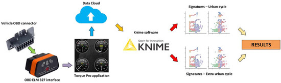
Figure 1.
Data flow in the research experiment.
The Torque Pro application is very helpful in conducting scientific research [51]. It is used by both academics and students. Using the application, the current values of selected parameters of the internal combustion engine can be displayed and saved to a file. These include, among others, the following parameters:
- -
- Engine RPM;
- -
- Calculated load value;
- -
- Coolant temperature;
- -
- Vehicle speed;
- -
- and many others.
The stability of the proposed system of measurement, acquisition, and processing of measurement data was very high. It took some time to install and pair the devices, but the system worked very stably afterwards. The authors repeatedly used the measurement system during short trips in urban conditions as well as long hours of highway driving. The stability of the entire system was greatly affected by access to the GPS system, which generated some of the measurement data. There were cases of GPS signal loss while driving through long tunnels. Therefore, the authors decided to record the speed of the vehicle using both the GPS and the vehicle’s OBD system. The stability of the vehicle’s OBD system was very high. Saved data files were not large in size and were processed very quickly by the software.
5. Road Tests of a Low-Emission LPG Vehicle under Urban Driving Conditions
The Torque Pro application was installed on a mobile tablet device. Almost every such device has a GPS communication module. Using the application, the scientists were able to save the values of the selected engine operating parameters and the position of the vehicle from the GPS system to a file. This made it possible to track the position of the vehicle during the road tests.
During the tests, the car travelled over 7 km. During the tests, the car travelled several kilometers in a typical urban cycle. An interesting solution was the overlay of the route on Google Maps and the use of a color scale to indicate the speed of travel, as shown in Figure 2. The green and yellow colors indicated low and medium speeds, while the orange and red colors indicated high speeds. The presented map clearly shows in which moments and on which sections the tested vehicle was moving at low and high speeds [52]. The maximum speed achieved by the vehicle was 77.26 km/h.
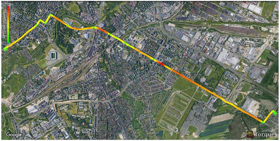
Figure 2.
The route during road tests in urban conditions. Distance: 7.39 km, time: 17 min.
The data collected during road tests of the vehicle were saved in *.csv format. For this reason, they could be easily displayed using a spreadsheet and useful graphs could be created (Table A1).
Graphs were created based on the data from the text file, examples of which are shown in Figure 3. Each graph showed the time course of a different parameter. In this case, eight main pieces of information from the sensors were taken into account:
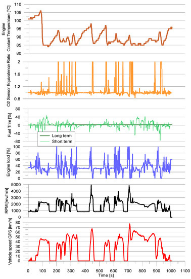
Figure 3.
Urban driving data displayed in graphs.
- -
- Device time [s],
- -
- Engine coolant temperature [°C];
- -
- Engine load [%];
- -
- Engine RPM [rev/min];
- -
- Fuel trim bank 1 long-term [%];
- -
- Fuel trim bank 1 short-term [%];
- -
- O2 sensor1 equivalence ratio [-];
- -
- Speed (GPS) [km/h].
The data collected during the road tests could be displayed in the form of useful graphs. Such examples are shown in Figure 3. On the basis of the selected engine operation parameters over time, it was already possible to determine the correct operation of the internal combustion engine in the tested vehicle. Even more useful information could be obtained by subjecting the measurement data to processing using artificial intelligence.
6. Marking the Route Signature in Urban Driving Conditions
For the offline data analysis, the authors used KNIME version 4.5.1 software. At the beginning of the work, all libraries necessary for the calculations were imported. Then, the measurement data were also imported.
The signature of the analyzed route was conceptualized as a trajectory in the state space. States were defined as clusters, which were created based on the following parameters:
- -
- Speed;
- -
- Engine load;
- -
- Acceleration.
To perform computations using the Python library, it was decided to choose from 5 to 10 clusters that formed the state space of the analyzed process—in the first case, there were five different states in the process, in the second case, there were 10. The trajectory of the analyzed process ran through separate states and the process signature was defined as a trajectory in the state space. In fact, the signature of the route should be generalized, taking into account the context in which the survey takes place. It can be generalized in terms of the driver of the vehicle, the type of route, or the time of day. Driving can occur on the same route, but during or off peak times, on a weekday, or on the weekend [53,54].
Thus, the aim of this article was to present a method of constructing signatures based on process data. The basis of this activity was the functions of the Internet of Things, which are present in the latest vehicles and allow processes to be recorded in the form of a multidimensional time series.
The K-Means method was used in the variant without prior data labelling (unsupervised learning without labelling) to determine clusters identified with process states. This approach was needed in the further validation of the results by determining whether the distinguished states (clusters) corresponded to the states of the process resulting from the expert understanding of the essence of the driving process.
The results of the basic statistical analysis of the data from driving in urban conditions are presented in Table 1.

Table 1.
Results of statistical analysis of data from driving in urban conditions.
Then, scatterplots were generated for the measured quantities (Chart table, Figure A5). The histograms across the diagonal of the figure displayed how often a given value occurred while driving.
Figure 4 shows scatterplots of the relationship between the selected measured values as well as histograms. From the scatterplots, the range of measurement data could be instantly read and concentration of the measurement data in the entire field could be predefined. The histograms represented how often a given value occurred while driving. They showed that during road tests on the analyzed section, the engine worked in the entire load range from 0% to 100%, but the largest share was the work with an average load of 40%.
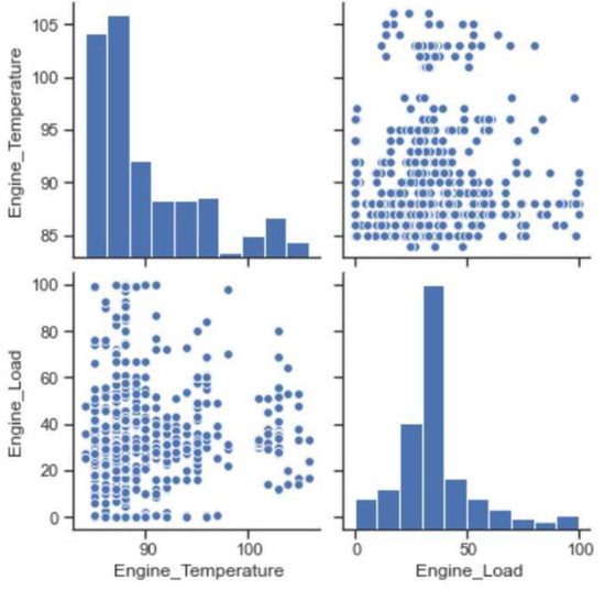
Figure 4.
Scatterplots and histograms.
Table 2 displays the matrix of inter-correlations between the measured quantities. There was a strong correlation between driving speed and engine load.
Table 2.
Correlation matrix.
The computing platform allowed the time course of the individual measurement data to be displayed, as shown in Figure 5.
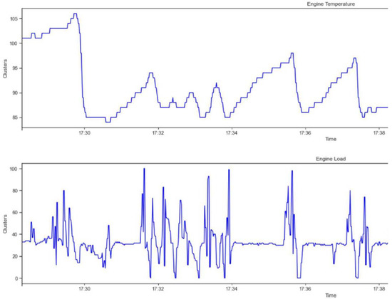
Figure 5.
Time course of engine temperature and load.
Data classification into five clusters (cluster numbers 0 to 4) is presented in Table 3. It is worth noting that the created clusters made physical sense. They could be attributed to terms commonly known in engine and automotive practice. For example, cluster 0 could be described as driving at a constant average speed of 44 km/h at an engine speed of 2231 rpm. Cluster 1 was defined as idling. This was indicated by the idling engine speeds and driving speeds close to 0 km/h. Cluster 3 included the strong acceleration that usually occurred when starting off and reaching speed in city traffic.
Table 3.
Travel speed and acceleration rotation centroids for five clusters.
Then, the trajectories of transition states were generated (Figure 6), corresponding to the five-cluster state classification. Calculations leading to the determination of the trajectory of the process in the state space allowed the probability of transitions between individual states to be determined as well as the probable distribution of the time spent in individual states.
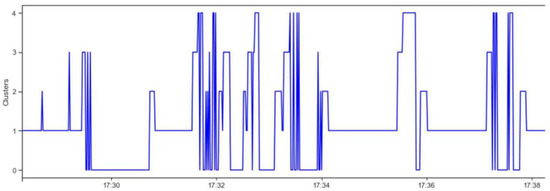
Figure 6.
Transition diagram corresponding to the five-cluster state classification.
How many times a process passed from a given state to another is identified in Table 4. The time spent in each state and the sequence of transitions are included in Table 5.
Table 4.
Table of transition results corresponding to the five-cluster classification of states.
Table 5.
Time spent in individual states and the order of transitions.
The oscillation of transitions in the five-degree state space is shown in Figure 7.
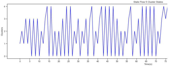
Figure 7.
Oscillation of transitions in the five-degree state space.
The appearances of the empirical densities of the probability distributions for individual states (clusters) are presented in Figure 8 and Figure 9. These graphs allowed us to easily detect the clusters defined in Table 3. Additionally, they were marked with appropriate colors. Cluster 0, corresponding to stable driving at medium speeds, was marked in blue. In the clusters of blue points, driving in individual gears could be easily observed. Cluster 1, defined as idling, was marked in orange. It was characterized by driving speeds close to 0 km/h and accelerations close to 0. However, expert knowledge was required for such an interpretation. The authors’ intention was to use artificial intelligence methods as much as possible in determining route signatures. The expert knowledge in the presented study was limited to the selection of the quantities defining the information space of the tested driving process, i.e., engine revolutions, driving speed and acceleration, as well as engine load.
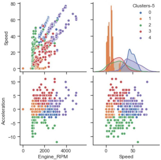
Figure 8.
Scatterplots of states and probability distribution densities for selected variables.
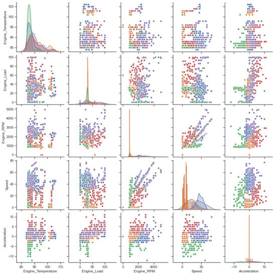
Figure 9.
Scatterplots of measurement data with process states marked in different colors.
7. Road Tests of a Low-Emission LPG Vehicle in Extra-Urban Driving Conditions
The next stage of the research was the execution of the route in extra-urban driving conditions. The journey took 1 h and 39 min. During this time, the vehicle travelled 110.03 km. The exact course of the route from Google Maps is shown in Figure 10. The route was exported from the Torque Pro software. Additionally, a color scale was used to denote the driving speed in this figure. The green and yellow colors indicated low and medium driving speeds, while the orange and red colors indicated high driving speeds [55]. The presented map clearly showed in which moments and on which sections the tested vehicle was moving at low and high speeds.
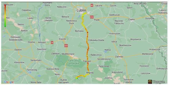
Figure 10.
The route during road tests in extra-urban conditions. Distance: 110.03 km, Time: 1 h, 39 min.
The graph in Figure 11 shows the raw measurement data, which could only be interpreted by an automotive expert. Performing even a simple statistical analysis allowed specific information to be obtained. The determination of the minimum, maximum, and average values, as well as the standard deviation already enabled the preliminary determination of the driving conditions.
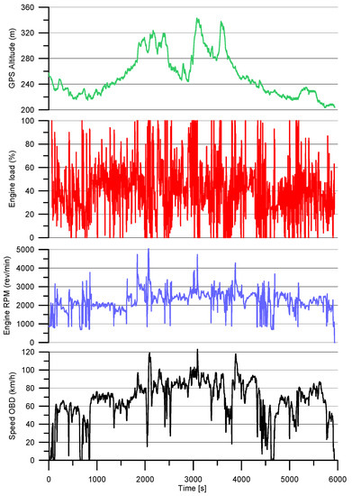
Figure 11.
Extra-urban driving data displayed in graphs.
The results of the basic statistical analysis of the data from driving in extra-urban conditions are presented in Table 6. The statistical analysis showed that the non-urban route was not at all easy. From the messages received from the driver and confirmed by marking the route on the map (see Figure 10), it appeared that the route took place through the Lublin Upland. Statistical analysis provided additional information about the minimum and maximum altitudes above sea level, which were 203 and 343 m above sea level, respectively. It followed that the level difference was significant and amounted to 140 m.
Table 6.
Results of statistical analysis of driving data in extra-urban conditions.
8. Marking the Route Signature in Extra-Urban Driving Conditions
Then, the data were classified into n = 5 states for extra-urban driving conditions. The altitude above sea level as a function of travel time is shown in Figure 12. Again, the system was marked with different colors and the affiliation into five clusters, which were numbered from 0 to 4. The presented data showed that the vehicle, at the beginning of its journey, made a descent from a small hill on which it was located in the city of Lublin and then it rose several times at an altitude of over 300 m above sea level. At present, even an expert found it difficult to make a physical interpretation of the generated cluster spaces. However, observant readers may notice that yellow and green colors predominated at lower altitudes, whereas blue and red colors prevailed at higher altitudes.
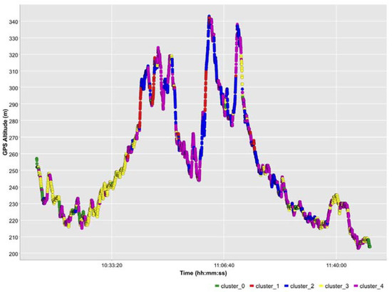
Figure 12.
Location above sea level as a function of travel time.
The authors decided to record the data on vehicle speed from two sources. The first was the OBD system and the second was the GPS satellite positioning system. Figure 13 shows that there was a very large correlation between these data, but its calculation was not important at the moment. The greater correlation was clearly noticeable at higher speeds, while a smaller correlation was observed at lower speeds. The authors considered the speed obtained from the GPS system to be more accurate. The speed obtained from the OBD system was less accurate and depended on the size of the rims, tire size, or even the pressure in the tires.
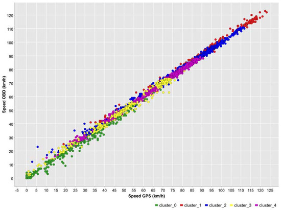
Figure 13.
Dependence of OBD-based driving speed on GPS-based driving speed.
The representation of individual states (clusters) was best illustrated by the diagram shown in Figure 14, indicating the dependence of the engine rotational speed on the engine load. The chart shows that the main determinant, but not the only clustering, was the engine speed. The states defined by cluster 0 were marked in green and contained engine speed points in the state space in the range from 0 to about 1400 rpm. The states defined by cluster 1 were marked in yellow and contained engine speed points in the state space ranging from about 1400 to about 2100 rpm. The states defined by cluster 2 were marked in pink and contained engine speed points in the state space ranging from about 2100 to about 2500 rpm. The states defined by cluster 3 were marked in blue and contained engine speed points in the state space ranging from about 2500 to about 3200 rpm. The states defined by cluster 4 were marked in red and contained engine speed points in the state space in the range from about 3200 to about 6000 rpm, which was the maximum obtained engine speed. Similar state limits determined by the engine rotational speed can be seen in Figure 15, showing the dependence of the driving speed on the rotational speed of the engine. We already noticed a similar dependence in the graph in Figure 8. However, in the case of extra-urban driving, it was even more clearly visible, because it was visualized using a much larger number of measurement points. From Table 2, we also learned that the strongest correlation was between the driving speed and the engine rpm, which was 0.81 for urban driving conditions.
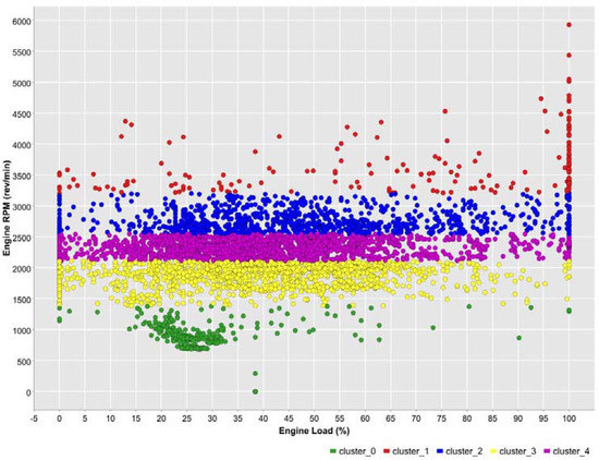
Figure 14.
Dependence of engine speed on engine load.
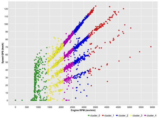
Figure 15.
Dependence of driving speed on engine rotational speed.
The strong correlation between driving speed and engine speed was due to the mechanical design of the vehicle driveline with a manual five-speed gearbox. The smallest correlation occurred between the parameters for gears 1, 2, and 3. The strongest and most visible correlation occurred for gears 4 and 5. This was due to the general characteristics of extra-urban driving. Apart from the initial acceleration of the vehicle, the driver did not use lower gears at all or very rarely, i.e., gears 1 and 2. Sometimes, the driver only used the reduction to gear 3 on long and steep climbs.
The graphs of the parameters shown in Figure 16 and Figure 17 showed that the condition corresponding to cluster 4 (marked in red) usually occurred during steep ascents to high altitudes. This was additionally confirmed by the data presented in Figure 12.
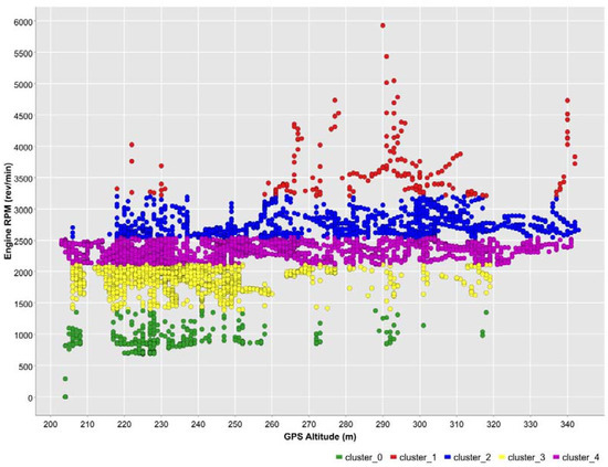
Figure 16.
Dependence of engine rotational speed on height above sea level.
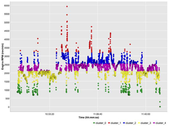
Figure 17.
Engine rotational speed as a function of travel time.
The relationship between the driving speed obtained from the GPS and the engine load is shown in Figure 18. In the case of city driving, there was a very small correlation between these parameters. Additionally, a very small correlation between these parameters occurred in urban driving conditions (see Table 2). Despite the lack of correlation between the driving speed obtained from the GPS and the engine load, clear clusters of points belonging to individual states (clusters) were noticeable. This was confirmed by the assumption made earlier that clustering was not based solely on the engine speed.
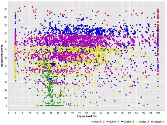
Figure 18.
Dependence of GPS-based driving speed on engine load.
The dependence of the driving speed on the rotational speed of the engine and its load is shown in Figure 19. The 3D visualization clearly showed the spatial distribution of the measurement points.
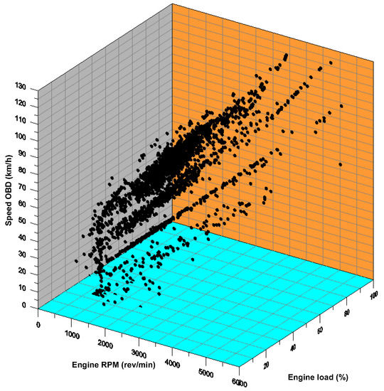
Figure 19.
Dependence of driving speed on engine rotational speed and its load.
The dependence of the driving speed on the engine rotational speed and the altitude above sea level is shown in Figure 20. Unfortunately, the results of clustering presented earlier could not be visualized with the help of 3D charts.
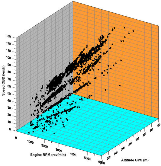
Figure 20.
Dependence of driving speed on engine rotational speed and height above sea level.
9. Summary and Conclusions
The article presents the possibilities of acquiring and processing measurement data from the OBD system of a spark-ignition vehicle converted to LPG. The software functions for communication with the aforementioned OBD and GPS systems were also demonstrated and described. The authors showed an interesting usage of data from both data sources. Moreover, their mutual use and processing were shown. The authors also focused on methods of effective visualization of the obtained data. This approach facilitated the interpretation of the obtained results by an expert from the automotive and transport industry. However, the specific aim of the article was to process the data from the vehicle and analyze the results using artificial intelligence methods.
In this article, the reference of the route was defined as the trajectory of the driving process, represented by the engine rotational speed, driving speed, and acceleration in the state space. The state space was separated based on the results of the cluster analysis. In the experiment, from the classification conducted for n classes, n = 5 was selected for both urban and extra-urban driving conditions. The K-Means algorithm was employed to determine the clusters in the variant without prior labelling of the classes using the teaching method and without participation of the teacher. The trajectories of the driving process in the five-state state space were determined. The class of each data record, the frequency of process switching between each pair of states, and the time spent in each state were determined.
The authors noticed some limitations in the system’s operation. The first was the ability to record only six engine and vehicle operating parameters at the same time. This limitation was due to the capabilities of the Torque Pro application. However, this limitation forced the authors to optimize the selection of appropriate engine and vehicle operating parameters. Another limitation was the loss of the GPS signal while driving through long underground tunnels. The authors compared the driving speed indications from both sources and it turned out that they were highly correlated. It was also a challenge to determine the number of clusters needed to create the signatures. The authors conducted research for 5 and 10 clusters. The division into five clusters turned out to be more useful. The number of clusters may become the subject of optimization studies. Another limitation may be the inability to obtain measurement data from the OBD systems of older vehicles manufactured before the year 2000.
The results of the analysis can be used to construct a probabilistic representation of the process in the form of a Bayesian network. Bayesian networks are one of the methods of artificial intelligence characterized by continuous updating of the process model through machine learning on process data and then reasoning through inferential, predictive, and diagnostic algorithms. In some applications, diagnostic reasoning would be necessary when filtering data in order to detect random disturbances in the course of the driving process (anomaly detection).
The proposed method of determining route signatures can have various applications. The use of algorithms without data labelling was used to validate individual classes of the movement process in urban and extra-urban traffic conditions. These classes can be used to compare trips made by different vehicles and on different routes. The authors are aware of the great potential of the presented data processing method for vehicle diagnostics and the description of driver behavior on the road. The tool used in the form of a Bayesian network is ideal for detecting all kinds of anomalies. This article is an introduction to a larger number of articles that will continue this research. The authors intend to compare the signatures of the same routes covered by different drivers using the same vehicle with simultaneous measurement of fuel consumption. This will identify the driver whose driving style provides the lowest fuel consumption and the greatest savings. Another interesting aspect may be the preparation of route signatures for various manners of urban driving (slow, dynamic, sporty) and determining their impact on road safety.
Author Contributions
Conceptualization, A.M. (Arkadiusz Małek) and J.C.; methodology, A.M. (Arkadiusz Małek), J.C., A.D. and A.M. (Andrzej Marciniak); software, A.M. (Arkadiusz Małek) and A.M. (Andrzej Marciniak); validation, A.M. (Arkadiusz Małek), J.C. and A.D.; formal analysis, A.M. (Arkadiusz Małek), A.D., and A.M. (Andrzej Marciniak); investigation, A.M. (Arkadiusz Małek), J.C., A.D., A.M. (Andrzej Marciniak) and J.V.; data curation, A.M. (Arkadiusz Małek), A.D. and A.M. (Andrzej Marciniak); writing—original draft preparation, A.M. (Arkadiusz Małek), J.C., A.D., A.M. (Andrzej Marciniak) and J.V.; writing—review and editing, A.M. (Arkadiusz Małek), J.C., A.D. and A.M. (Andrzej Marciniak); visualization, A.M. (Arkadiusz Małek), J.C. and J.V.; supervision, J.C. and J.V.; project administration, A.M. (Arkadiusz Małek) and J.C.; funding acquisition, A.D. All authors have read and agreed to the published version of the manuscript.
Funding
This research received no external funding.
Data Availability Statement
The study did not report any data.
Conflicts of Interest
The authors declare no conflict of interest.
Appendix A

Figure A1.
The object of the research in the form of a Renault Mégane vehicle with a low-emission LPG engine.

Figure A2.
Installation of LPG injectors.

Figure A3.
Toroidal LPG tank mounted in place of the spare wheel.

Figure A4.
Mounting location of LPG refueling valve.

Figure A5.
Scatterplots of the measured quantities.
Table A1.
Driving data saved to a text file.
Table A1.
Driving data saved to a text file.
| Engine Load (%) | Engine RPM (rpm) | Speed (GPS) (km/h) | Speed (OBD)(km/h) | GPS Altitude (m) | |
|---|---|---|---|---|---|
| 1 | 31.37 | 858 | 0 | 0 | 257 |
| 2 | 31.37 | 891.5 | 0 | 0 | 257 |
| 3 | 30.98 | 873 | 0 | 0 | 257 |
| 4 | 30.98 | 873 | 0 | 0 | 257 |
| 5 | 30.59 | 869 | 0 | 0 | 256 |
| 6 | 30.59 | 864 | 0 | 0 | 254 |
| 7 | 29.41 | 883.5 | 0 | 0 | 252 |
| 8 | 30.59 | 878.5 | 0 | 0 | 252 |
| 9 | 30.2 | 881 | 0 | 0 | 252 |
| 10 | 30.2 | 869 | 0 | 0 | 252 |
| 11 | 30.98 | 882 | 0 | 0 | 252 |
| 12 | 29.02 | 881.5 | 0 | 0 | 252 |
| 13 | 30.98 | 873.5 | 0 | 0 | 252 |
| 14 | 30.2 | 872.5 | 0 | 0 | 252 |
| 15 | 30.59 | 878 | 0 | 0 | 252 |
| 16 | 30.2 | 856 | 0 | 0 | 252 |
| 17 | 30.59 | 872 | 0 | 0 | 252 |
| 18 | 30.2 | 860 | 0 | 0 | 252 |
| 19 | 29.8 | 889 | 0 | 0 | 252 |
| 20 | 30.2 | 869.5 | 0 | 0 | 252 |
| 21 | 29.8 | 872 | 0 | 0 | 252 |
| 22 | 30.59 | 881 | 0 | 0 | 252 |
| 23 | 29.8 | 853 | 0 | 0 | 252 |
| 24 | 30.98 | 849 | 0 | 0 | 252 |
| 25 | 30.59 | 853.5 | 0 | 0 | 252 |
| 26 | 29.41 | 877.5 | 0 | 0 | 252 |
| 27 | 38.43 | 876.5 | 0 | 0 | 252 |
| 28 | 27.84 | 1326.5 | 0 | 0 | 252 |
| 29 | 29.41 | 1142 | 0 | 0 | 252 |
| 30 | 41.57 | 1105 | 0 | 0 | 252 |
| 31 | 57.65 | 1395.5 | 0 | 0 | 252 |
References
- Borawski, A.; Mieczkowski, G.; Szpica, D. Composites in Vehicles Brake Systems-Selected Issues and Areas of Development. Materials 2023, 16, 2264. [Google Scholar] [CrossRef] [PubMed]
- Faraj, R.; Graczykowski, C.; Hinc, K.; Holnicki-Szulc, J.; Knap, L.; Senko, J. Adaptable pneumatic shock-absorber. In Proceedings of the 8th Conference on Smart Structures and Materials, SMART 2017 and the 6th International Conference on Smart Materials and Nanotechnology in Engineering, SMN 2017, Madrid, Spain, 5–8 June 2017; pp. 86–93. [Google Scholar]
- Jilek, P.; Němec, J. System for Changing Adhesion Conditions in Experimental Road Vehicle. Int. J. Automot. Technol. 2021, 22, 779–785. [Google Scholar] [CrossRef]
- Rybicka, I.; Droździel, P.; Komsta, H. Assessment of the Braking System Damage in the Public Transport Vehicles of a Selected Transport Company. Period. Polytech. Transp. Eng. 2023, 51, 172–179. [Google Scholar] [CrossRef]
- Sejkorová, M.; Verner, J.; Sejkora, F.; Hurtová, I.; Senkýr, J. Analysis of operation wear of brake fluid used in a Volvo car. In Proceedings of the International Conference 2018: Transport Means, Trakai, Lithuania, 3–5 October 2018; Kaunas University of Technology: Kaunas, Lithuania, 2018; pp. 592–596. [Google Scholar]
- Stopka, O.; Kampf, R.; Vrábel, J. Deploying the means of transport within the transport enterprises in the context of emission standards. In Proceedings of the 20th International Scientific Conference Transport means, Kaunas University of Technology, Juodkrante, Lithuania, 5–7 October 2016; pp. 185–190. [Google Scholar]
- Mądziel, M.; Campisi, T. Investigation of Vehicular Pollutant Emissions at 4-Arm Intersections for the Improvement of Integrated Actions in the Sustainable Urban Mobility Plans (SUMPs). Sustainability 2023, 15, 1860. [Google Scholar] [CrossRef]
- Mikulski, M.; Drozdziel, P.; Tarkowski, S. Reduction of transport-related air pollution. A case study based on the impact of the COVID-19 pandemic on the level of NOx emissions in the city of Krakow. Open Eng. 2021, 11, 790–796. [Google Scholar] [CrossRef]
- Ziółkowski, A.; Fuć, P.; Lijewski, P.; Jagielski, A.; Bednarek, M.; Kusiak, W. Analysis of Exhaust Emissions from Heavy-Duty Vehicles on Different Applications. Energies 2022, 15, 7886. [Google Scholar] [CrossRef]
- Dittrich, A.; Beroun, S. Spark Plug with Integrated Chamber. MATEC Web Conf. 2018, 220, 04005. [Google Scholar] [CrossRef]
- Hurtová, I.; Sejkorová, M. Determination of the octane number of automotive gasolines by ftir spectrometry with chemometrics. Perner’s Contacts 2022, 17. [Google Scholar] [CrossRef]
- Szpica, D. Combustion Systems and Fuels Used in Engines—A Short Review. Appl. Sci. 2023, 13, 3126. [Google Scholar] [CrossRef]
- Fabiś, P.; Flekiewicz, M. Optimalisation of the SI Engine Timing Advance Fueled by LPG. Sci. J. Sil. Univ. Technol. Ser. Transp. 2021, 111, 33–41. [Google Scholar] [CrossRef]
- Kriaučiūnas, D.; Pukalskas, S.; Rimkus, A.; Barta, D. Analysis of the influence of CO2 concentration on a spark ignition engine fueled with biogas. Appl. Sci. 2021, 11, 6379. [Google Scholar] [CrossRef]
- Manko, I.; Matijošius, J.; Shuba, Y.; Rimkus, A.; Gutarevych, S.; Slavin, V. Using Mathematical Modeling to Evaluate the Performance of a Passenger Car When Operating on Various Fuels. Energies 2022, 15, 6343. [Google Scholar] [CrossRef]
- Szpica, D.; Kusznier, M. Computational Evaluation of the Effect of Plunger Spring Stiffness on Opening and Closing Times of the Low-Pressure Gas-Phase Injector. Mechanika 2022, 28, 242–246. [Google Scholar] [CrossRef]
- Šmigins, R.; Kryshtopa, S.; Pajak, M. Impact of Low Level N-butanol and Gasoline Blends on Engine Performance and Emission Reduction. In Proceedings of the Transport Means-Proceedings of the International Conference, Online, 6–8 October 2021; pp. 481–486. [Google Scholar]
- Tuan, N.T.; Dong, N.P. Improving Performance and Reducing Emissions from a Gasoline and Liquefied Petroleum Gas Bi-Fuel System Based on a Motorcycle Engine Fuel Injection System. Energy Sustain. Dev. 2022, 67, 93–101. [Google Scholar] [CrossRef]
- Regulation No 115 of the Economic Commission for Europe of the United Nations (UN/ECE). Available online: https://eur-lex.europa.eu/legal-content/EN/TXT/PDF/?uri=CELEX:42014X1107(02) (accessed on 21 March 2023).
- Hanzl, J.; Pečman, J.; Bartuška, L.; Stopka, O.; Šarkan, B. Research on the Effect of Road Height Profile on Fuel Consumption during Vehicle Acceleration. Technologies 2022, 10, 128. [Google Scholar] [CrossRef]
- Jereb, B.; Stopka, O.; Skrúcaný, T. Methodology for Estimating the Effect of Traffic Flow Management on Fuel Consumption and CO2 Production: A Case Study of Celje, Slovenia. Energies 2021, 14, 1673. [Google Scholar] [CrossRef]
- Mikulski, M.; Wierzbicki, S.; Pietak, A. Numerical studies on controlling gaseous fuel combustion by managing the combustion process of diesel pilot dose in a dual-fuel engine. Chem. Process Eng. Inz. Chem. I Proces. 2015, 36, 225–238. [Google Scholar] [CrossRef]
- Osipowicz, T.; Abramek, K.F.; Barta, D.; Drozdziel, P.; Lisowski, M. Analysis of possibilities to improve environmental operating parameters of modern compression-ignition engines. Adv. Sci. Technol. Res. J. 2018, 12, 206–213. [Google Scholar] [CrossRef]
- Skrúcaný, T.; Kendra, M.; Čechovič, T.; Majerník, F.; Pečman, J. Assessing the Energy Intensity and Greenhouse Gas Emissions of the Traffic Services in a Selected Region. LOGI-Sci. J. Transp. Logist. 2021, 12, 25–35. [Google Scholar] [CrossRef]
- Słowiński, P.; Burdzik, R.; Juzek, M.; Turoń, K.; Czech, P. Ecological and economic aspects of transport activities from the point of view of fuel economy of vehicles. In Proceedings of the Transport Means-Proceedings of the International Conference, Juodkrante, Lithuania, 20–22 September 2017; pp. 829–834. [Google Scholar]
- Dziewiątkowski, M.; Szpica, D. Analysis of the Influence of the Selective Reduction System (SCR) Application for a Diesel Engine on the Emission Level of Nitrogen Oxides (NOx). In Proceedings of the Transport Means-Proceedings of the International Conference, Online, 5–7 October 2022; pp. 74–78. [Google Scholar]
- Giakoumis, E.G.; Zachiotis, A.T. Investigation of a Diesel-Engine Vehicle’s Performance and Emissions during the WLTC Driving Cycle—Comparison with the NEDC. Energies 2017, 10, 240. [Google Scholar] [CrossRef]
- Gołębiowski, W.; Wolak, A.; Zając, G. The influence of the presence of a diesel particulate filter (DPF) on the physical and chemical properties as well as the degree of concentration of trace elements in used engine oils. Pet. Sci. Technol. 2019, 37, 746–755. [Google Scholar] [CrossRef]
- Kwon, S.; Park, Y.; Park, J.; Kim, J.; Choi, K.H.; Cha, J.S. Characteristics of on-road NOx emissions from Euro 6 light-duty diesel vehicles using a portable emissions measurement system. Sci. Total Environ. 2017, 576, 70–77. [Google Scholar] [CrossRef] [PubMed]
- O’Driscoll, R.; Stettler, M.E.J.; Molden, N.; Oxley, T.; ApSimon, H.M. Real world CO2 and NOx emissions from 149 Euro 5 and 6 diesel, gasoline and hybrid passenger cars. Sci. Total Environ. 2018, 621, 282–290. [Google Scholar] [CrossRef] [PubMed]
- Rybicka, I.; Stopka, O.; L’upták, V.; Chovancová, M.; Droździel, P. Application of the methodology related to the emission standard to specific railway line in comparison with parallel road transport: A case study. MATEC Web Conf. 2018, 244, 03002. [Google Scholar] [CrossRef]
- Šarkan, B.; Loman, M.; Synák, F.; Skrúcaný, T.; Hanzl, J. Emissions Production by Exhaust Gases of a Road Vehicle’s Starting Depending on a Road Gradient. Sensors 2022, 22, 9896. [Google Scholar] [CrossRef]
- Pechout, M.; Dittrich, A.; Mazac, M.; Vojtisek-Lom, M. Real Driving Emissions of Two Older Ordinary Cars Operated on High-Concentration Blends of N-Butanol and ISO-Butanol with Gasoline. SAE Tech. Pap. 2015, 24, 2488. [Google Scholar] [CrossRef]
- Hlatka, M.; Bartuska, L. Comparing the Calculations of Energy Consumption and Greenhouse Gases Emissions of Passenger Transport Service. Nase More 2018, 65, 224–229. [Google Scholar] [CrossRef]
- Procházka, R.; Dittrich, A.; Beroun, S.; Zvolský, T.; VoŽenílek, R. The Working Cycle of the Motoring Internal Combustion Engine by a New Method with Cylinder Pressures as in Real Engine Operation. Stroj. Cas. 2022, 72, 41–52. [Google Scholar] [CrossRef]
- Šarkan, B.; Hudec, J.; Sejkorova, M.; Kuranc, A.; Kiktova, M. Calculation of the production of exhaust emissions in the laboratory conditions. J. Phys. Conf. Ser. 2021, 1736, 012022. [Google Scholar] [CrossRef]
- Koszałka, G.; Szczotka, A.; Suchecki, A. Comparison of fuel consumption and exhaust emissions in WLTP and NEDC procedures. Combust. Engines 2019, 179, 186–191. [Google Scholar] [CrossRef]
- Pavlovic, J.; Ciuffo, B.; Georgios, F.; Valverde, V.; Marotta, A. How much difference in type-approval CO2 emissions from passenger cars in Europe can be expected from changing to the new test procedure (NEDC vs. WLTP)? Transp. Res. Part A Policy Pract. 2018, 111, 136–147. [Google Scholar] [CrossRef]
- Kaźmierczak, A.R.; Matla, J. Method of verifying the emission level of the exhaust components of a special vehicle in relation to EURO III standard in road conditions. Combust. Engines 2022, 61, 89–93. [Google Scholar] [CrossRef]
- Sharma, A.; Podoplelova, E.; Shapovalov, G.; Tselykh, A.; Tselykh, A. Sustainable Smart Cities: Convergence of Artificial Intelligence and Blockchain. Sustainability 2021, 13, 13076. [Google Scholar] [CrossRef]
- Keertikumar, M.; Shubham, M.; Banakar, R.M. Evolution of IoT in smart vehicles: An overview. In Proceedings of the 2015 International Conference on Green Computing and Internet of Things (ICGCIoT), Greater Noida, India, 8–10 October 2015; pp. 804–809. [Google Scholar] [CrossRef]
- Witaszek, K. Modeling of fuel consumption using artificial neural networks. Diagnostyka 2020, 21, 103–113. [Google Scholar] [CrossRef]
- Devi, Y.U.; Rukmini, M.S.S. IoT in connected vehicles: Challenges and issues—A review. In Proceedings of the 2016 International Conference on Signal Processing, Communication, Power and Embedded System (SCOPES), Paralakhemundi, India, 3–5 October 2016; pp. 1864–1867. [Google Scholar] [CrossRef]
- Lasocki, J.; Chłopek, Z.; Godlewski, T. Driving style analysis based on information from the vehicle’s OBD system. Combust. Engines 2019, 58, 173–181. [Google Scholar] [CrossRef]
- Pourrahmani, H.; Yavarinasab, A.; Zahedi, R.; Gharehghani, A.; Mohammadi, M.H.; Bastani, P.; Van Herle, J. The applications of Internet of Things in the automotive industry: A review of the batteries, fuel cells, and engines. Internet Things 2022, 19, 100579. [Google Scholar] [CrossRef]
- Puchalski, A.; Komorska, I. Driving style analysis and driver classification using OBD data of a hybrid electric vehicle. Transp. Probl. 2020, 15, 83–94. [Google Scholar] [CrossRef]
- Lejda, K.; Kurczyński, D.; Łagowski, P.; Warianek, M.; Dąbrowski, T. The evaluation of the Fiat 0.9 TwinAir engine powered by petrol and LPG gas work cycles uniqueness. J. KONES 2018, 25, 323–330. [Google Scholar] [CrossRef]
- Jaworski, A.; Lejda, K.; Lubas, J.; Madziel, M. Comparison of exhaust emission from Euro 3 and Euro 6 motor vehicles fueled with petrol and LPG based on real driving conditions. Combust. Engines 2019, 58, 106–111. [Google Scholar] [CrossRef]
- Kmieć, M.; Weber, M.; Romijn, M.; Matthews, D. Application of automotive safety design methodologies to the development of Euro 7 emission control systems including on board monitoring. Combust. Engines 2022, 61, 75–82. [Google Scholar] [CrossRef]
- Available online: https://allegro.pl/oferta/obd2-interfejs-bluetooth-3-0-polski-diagnostyczny-9002958407?utm_feed=aa34192d-eee2-4419-9a9a-de66b9dfae24&utm_source=google&utm_medium=cpc&utm_campaign=_mtrzcj_narzedzia_pla_pmax&ev_campaign_id=17996380314&gclid=CjwKCAjw6IiiBhAOEiwALNqnccC6xC8yGR8Ypqo7_wgFzRJc1ArL9-z6h4RSpB1PsfIPNm_DsGHm9hoCsmsQAvD_BwE (accessed on 21 April 2023).
- Torque Pro (OBD 2 & Car). Available online: https://play.google.com/store/apps/details?id=org.prowl.torque&hl=pl (accessed on 17 October 2022).
- Cieślik, W.; Szwajca, F.; Golimowski, J. The possibility of energy consumption reduction using the ECO driving mode based on the RDC test. Combust. Engines 2020, 59, 59–69. [Google Scholar] [CrossRef]
- Engelmann, D.; Hüssy, A.; Comte, P.; Czerwinski, J.; Bonsack, P. Influences of special driving situations on emissions of passenger cars. Combust. Engines 2021, 60, 41–51. [Google Scholar] [CrossRef]
- Chang, H.; Ning, N. An Intelligent Multimode Clustering Mechanism Using Driving Pattern Recognition in Cognitive Internet of Vehicles. Sensors 2021, 21, 7588. [Google Scholar] [CrossRef] [PubMed]
- Nowak, M.; Kamińska, M.; Szymlet, N. Determining if Exhaust Emission From Light Duty Vehicle During Acceleration on The Basis of On-Road Measurements and Simulations. J. Ecol. Eng. 2021, 22, 63–72. [Google Scholar] [CrossRef]


Disclaimer/Publisher’s Note: The statements, opinions and data contained in all publications are solely those of the individual author(s) and contributor(s) and not of MDPI and/or the editor(s). MDPI and/or the editor(s) disclaim responsibility for any injury to people or property resulting from any ideas, methods, instructions or products referred to in the content. |
© 2023 by the authors. Licensee MDPI, Basel, Switzerland. This article is an open access article distributed under the terms and conditions of the Creative Commons Attribution (CC BY) license (https://creativecommons.org/licenses/by/4.0/).