Abstract
This paper proposes a nonlinear flux linkage observer for the PMSM speed controls without motion sensors, introducing the deviation among the real stator flux linkage and an estimated stator flux linkage to suppress feedback and integral flux drift. In the position detection of an interior PMSM without a speed sensor, the traditional back EMF integration method uses a pure integrator, or LPF, to estimate the stator flux. Its inherent defects inevitably lead to inaccurate flux estimation, which directly affects the estimation of the motor mover position, resulting in the decline in motor control operation and the distortion of phase current. This paper uses an improved integrator with adaptive compensation. The projected value of the stator flux linkage has been derived from the estimated value of the rotor permanent magnetic flux linkage position angle and the algebraic model (m-model) of the stator flux linkage, along with a synchronous coordinate system. The IPMSM stator coil flux linkage obtained from the stator coil current and integral voltage models in the static coordinate system is compared to form a feedback closed-loop to suppress the integral drift, and using the cross-product approach of the actual and estimated flux linkage yields the projected value of the IPMSM rotor speed and position through a PLL. Compared with the existing motion-sensorless observers, the methodology proposed in this article is simple and exhibits better dynamic and static estimation performance. Extensive and comprehensive MATLAB computer simulation and experimental findings validate the proposed motion-sensorless control mechanism.
1. Introduction
With the development of high-performance permanent magnet materials, power electronics devices technology, and microcontroller technology, the control and speed regulation performance of the permanent magnet synchronous motor (PMSM) is improving and is increasingly widely used [1]. In practical application, vector control is the most used control strategy for PMSM. Generally, rotor position and speed information are achieved by installing resolver or encoder sensors. However, the installation of sensors is restricted by environment, increased space, and system cost and is vulnerable to electromagnetic interference. Therefore, PMSM sensorless technology has been applied in harsh climates and in situations which are sensitive to system costs. The relevant theories and research methods have been studied in Ref. [2]. Even though the technology is an advanced, stable operation of ac drives, the extremely low-speed zone remains a critical issue due to the low back EMF.
The widely accepted motion-sensorless control algorithms of PMSM are mainly divided into algorithms ideal for moderate- and high-speed areas and algorithms suitable for low or even zero speed. A position sensorless control technique is perfect for application in the moderate- and high-speed range, including for flux estimation, the sliding mode observer (SMO), the model-reference adaptive approach, the extended Kalman filter, etc. [3,4,5,6]. These algorithms are generally used for permanent surface magnet synchronous motors (SPMSM). On the basis of the voltage flux mathematical model of SPMSM in static coordinates, the back EMF is obtained, and the position angle of the rotor is estimated through the arctangent function, or PLL. For the interior PMSM, due to the different inductance of the direct and quadrature axes, the inductance in the static coordinate system is a function of motor rotor angle position, which can make the design of the IPMSM sensorless control system much more difficult [7,8]. Refs. [7,8] analyze the reason why the sensorless control method, suitable for SPMSM, cannot be used for IPMSM, proposing an extended electromotive force (EEMF) model ideal for IPMSM. After estimating EEMF, the position estimation of rotor flux can be obtained from its phase, as is the case for the back EMF in SPMSM. The disturbance observer is employed in Ref. [7] to calculate the extended back EMF. The arctangent operation is utilized to compute the position of the rotor angle. The adaptive observer obtains the estimated speed to realize the motion-sensorless position control of interior PMSM. However, the parameter configuration method is complex, and the inverse tangent function is sensitive to noise, which can easily cause the deviation of rotor position estimation. The research in ref. [8], established on the extended back EMF model, uses the extended Kalman method to compute the estimated EEMF, obtains the rotor position through the arctangent operation, and realizes the motion-sensorless control of IPMSM. However, the design of the extended Kalman method is complex, the amount of calculation is extensive, and the variance matrix structure affects the algorithm’s convergence.
The above observation algorithm fails whenever the interior PMSM is at slow or zero speed because the back EMF is low or equivalent to zero. The motion-sensorless method of PMSM studied in the existing literature, at low velocity or even zero speed, mainly uses motor saliency to determine the position angle of the rotor. The most typical algorithm detects the high-frequency current response generated by a motor. It obtains the rotor’s position information by injecting voltage or current excitation far higher than the fundamental frequency of the IPMSM [9]. However, injecting high-frequency voltage or current will produce torque ripple. In addition to the above high-frequency injection method, some open-loop observation algorithms, such as V/F (voltage-frequency ratio) and I/F (current frequency ratio) control strategies, exist. Unfortunately, these algorithms are unsuitable for high dynamic response situations because they have no closed-loop system.
The EMF methodology is simple to implement and performs well across a broad speed range, and the EMF estimate method based on a least-order observer has been widely employed [10,11,12]. The least-order observer reconstructs the IPMSM voltage equation. This method is simple to develop, but increases speed and position inaccuracies due to the lack of self-feedback.
A pure integrator is a core part of the design of a classical rotor flux observer based on the PMSM voltage and flux models [13,14]. Mismatched parameters, an incorrect integral initial value, stator voltage, current detection faults, and converter interruption generate high-frequency harmonics and DC offset in computed flux. Consequently, the estimated rotor velocity and position angle are inaccurate due to the saturation effect because of the incorrect initial integral value [15]. As a result, certain studies have optimized the pure integration based on the rotor flux observer. In Refs. [14,15], a gradient approach based on an initial flux condition analyzer is designed to calculate the rotor flux compensation’s incorrect initial integral value [16,17], and new coefficient designs are used to strengthen the stability of the rotor flux observer. Ref. [18] proposes a disturbance observer that utilizes the stator flux integrator to obtain the rotor flux.
Due to the drift and saturation issues associated with back electromotive force (EMF) integration, the LPF is typically utilized in place of the pure integrator [14]. While this approach eliminates the DC component, phase shifts may occur in the projected equivalent rotor flux linkage. As a result, the proposed method cannot precisely determine the rotor speed and angular position. Ref. [19] uses a programmable cascaded LPF, which can theoretically overcome the mitigation of the DC offset. However, this method has stringent requirements for selecting the cut-off frequency of the cascaded LPF, and it is not easy to achieve ideal results in practice.
On the other hand, an SMO model is developed to enhance the precision and robustness of motor speed and position estimations. Due to its inherent resilience and simplicity, the sliding mode technique is a well-known and significant nonlinear control method. The “chattering effect”, which can generally be mitigated by employing an LPF, is the primary drawback of these approaches [4,20]. The motor speed and position are estimated using the SMO method based on the active flux principle [21]. When combined with high-frequency signal injection (HFSI), a zero-speed operation is achievable. In Ref. [22], the super-twisting algorithm was introduced to improve the performance of steady-state observation by reducing sliding mode chattering. The back-EMF 2nd-order sliding mode observer is developed using the active flux to reconstruct the voltage model based on the super-twisting technique.
Speed-adaptive full-order or reduced-order Luenberger observers are used to estimate the stator current and flux vectors [17,23,24]. The speed is computed by feeding the current error via a PI (proportional-integral) adaptation mechanism. A stable operation of a reduced-order position angle observer with stator resistance adaptation at 30 r/min with step load is reported in Ref. [17]. When combined with HFSI, a zero-speed operation is achievable [25].
The 2nd-order integral flux observer with the frequency-locked loop (SOIFO-FLL) approach is proposed in Ref. [26], reducing the amplitude, but not eliminating the DC offset. The direct current component and high-order frequency harmonic can be eliminated by a 2nd-order integral flux observer with the frequency-locked loop (SOIFO-FLL), as reported in Ref. [27]. A 2nd-order SOIFO-FLL computation process is complex. Additionally, an improved rotor flux observer was proposed in Ref. [28], reducing the DC offset and high-order frequency harmonics. However, this approach is ineffective during speed reversals and may result in significant position estimation inaccuracy. In addition, a novel PLL-type estimation scheme for the sensorless control of PMSM machines was proposed in Ref. [29]. The PLL observer employs the d-axis current error as an adjustment item for the 2nd-order PLL position observer and the q-axis current error for the third-order extended speed Luenberger observer to precisely control the motor speed in the absence of a position sensor. However, this method is highly dependent on motor parameters, and the control system is quite complex. Among the magnetic flux estimation methods, a paper applying the active magnetic flux concept has been published, showing that rotor position estimation is possible even in the slow-speed operation region [30,31]. Because the current estimation error is fed back to estimate the magnetic flux, it is mandatory to use a current estimator.
Nevertheless, the presented current estimator is relatively complex, and the position estimation performance deteriorates due to the error of the motor parameter [31]. The proposed motion-sensorless control approach applies to various industrial applications, including electric vehicles and servo systems. Its features include a broad speed range, easy implementation, and the potential to reduce DC components and high-order frequency harmonics. As a result, no additional parameter identification or disturbance suppression structures are required. Remarkably, the proposed method can be applied in the 1.0–100.0% range of rated speed. In contrast, 95.0% of motion-sensorless control techniques established on the back-EMF estimate are inefficient, i.e., below 5.0% of the rated speed.
This article presents an improved IPMSM position sensorless system design scheme. The projected value of the IPMSM stator flux linkage is calculated from an estimated value of the rotor permanent magnetic flux linkage angle and the algebraic model (m-model) of the stator flux linkage within a synchronous coordinate system. In the alpha-beta, () frame, the IPMSM stator flux linkages obtained from the stator voltage and the current integral models are compared to form a feedback closed-loop to suppress the integral drift. The estimated IPMSM rotor position angle/speed values are obtained using the cross-product of the actual and estimated flux linkage through the phase-locked loop. Compared with the existing motor rotor position angle/speed estimation methods, the methodology proposed in this article is simple and has better dynamic and static estimation performance. The MATLAB/Simulink and experimental outcomes show that the suggested speed estimation algorithm works effectively, regardless of the variation in machine parameters for different speed ranges and loads.
The structure of this article is as follows. Section 2 discusses the mathematical and stability analysis of the presented rotational position and speed estimation technique. The presented algorithm for a speed sensorless PMSM drive is implemented in MATLAB/Simulink, and preliminary findings are shown in Section 3. The Myway PE-expert4 -based PMSM drive laboratory prototype is used to verify the estimation method in the hardware. Section 4 presents the corresponding findings. The conclusion is presented in Section 5.
2. Theory and Application of Flux Observer with Phase Lock Loop
The stator flux measurement’s precision directly impacts the control system’s performance. In the high-performance PMSM sensorless control system, the pure integrator, with a simple structure, is employed to estimate the stator flux. Although the system structure is simplified, efficient, and easy to implement, and the reliance on motor parameters is reduced, the pure integrator observation method exhibits the initial value, DC offset, and current sampling problem, causing harmonics amplification. At the same time, because the pure integrator has no inhibitory effect on the DC component in the input signal, even a small DC component will eventually lead to the saturation of the integrator. While the motor is running, the direct current component can be created by sampling the stator current. Therefore, the typical flux observer cannot precisely determine the rotor’s speed and position. The LPF can solve the pure integrator problem in practical applications, but can also lead to amplitude and phase inaccuracies in observing stator flux compared with the actual flux. The inaccuracies may have an impact on the motor’s speed control performance. In the position sensorless PMSM system, this article proposed an improved flux observer design with a PLL, as shown in Figure 1. This article discusses its stability analysis and design methods.
Figure 1.
Design of the flux observer with a PLL in the position motion-sensorless system of PMSM.
In Figure 1,
, , , and are the -axis and -axis components of the stator voltage and stator current of the motor in the static coordinate system, respectively. is the estimated value of the motor rotor angle obtained by the phase-locked loop, i.e., the estimated value of the rotor permanent magnet flux linkage orientation angle; the corresponding coordinate system is called an estimated synchronous coordinate system, is the permanent magnet flux linkage of the motor, , and is the projection value of the stator current in the estimated synchronous coordinate system, ,,,; the calculation is as shown in Figure 1. , and is the stator flux obtained by integrating the voltage and current model of the motor; and are the projection values in the static coordinate system, , .
Because the phase-locked loop has two integral links, when the motor speed is constant (i.e., when the motor rotation angle is a ramp function of time), the static error of the phase-lock loop is equal to zero to establish a steady-state solution of the system at this time
Since the system has multiple equilibrium points, it cannot be globally asymptotically stable.
2.1. Stability Analysis of Flux Observer with the Phase-Locked Loop
Suppose the stator current of the motor is equal to zero (that is, no external load or field weakening current, hereafter referred to as no load), namely . The stator voltage , represents the electromotive force generated by the permanent magnets of the rotor rotating on the stator winding.
Defining the error signal
Appendix A contains the appropriate deduction of Equations (6) and (7). The error model (large-signal nonlinear model) is shown in Figure 2.
Figure 2.
A large-signal nonlinear model of the flux observer with a PLL.
The error model (large-signal nonlinear model) shown in Figure 2 is a nonlinear time-varying system in which the time-varying characteristic comes from the change of time, and the nonlinear characteristic comes from the cross-product and angle calculation. The following discussion mainly applies the stability analysis method based on passivity.
In Figure 2, , , the error model of Figure 2 can be further represented as shown by Figure 3. Near the origin
Figure 3.
The equivalent large-signal nonlinear model of the flux observer with a PLL.
Firstly, the linearized model (small signal model) near the steady-state operating point is given. It is linear and time-varying and cannot be used to analyze the stability by calculating the eigenvalue. However, it is difficult to solve the stability problem of the equilibrium point of the nonlinear time-varying system using the small gain theorem.
From Equation (9) above, the expression () is further derived to obtain the linearization model (small signal model) for the nonlinear model of the flux observer with a PLL, as follows
Similarly, from Equation (9) above, the expression is further derived to get the linearization model near the steady state, as follows
Based on Equations (9)–(11), Equation (12) is derived as follows
Thus, the linearization model near the steady state is shown in Figure 4.
Figure 4.
Small-signal linearization model near the steady-state.
The linearized model near the steady state, shown in Figure 4, can also be equivalently represented as the system in Figure 5. When the transfer function is strictly positive in real-time, and the signal vector satisfies the sufficient excitation condition, the origin of the system is asymptotically stable.
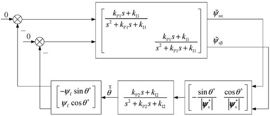
Figure 5.
The equivalent model of a small-signal model near the steady-state.
The stability problem of the large-signal nonlinear error model, shown in Figure 2 and Figure 3, is discussed below. For this reason, the error model in Figure 3 is expressed as an equivalent form in Figure 6.
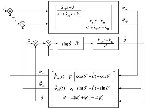
Figure 6.
The equivalent form of the error model (large signal error model).
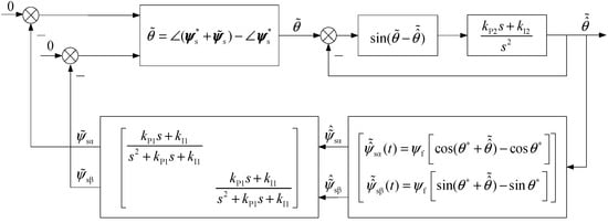
Figure 7.
The series form of the error model.
The typical phase-locked loop system in the upper right corner of Figure 7 is stable, with a static gain of 1, and there is enough bandwidth in the design to approximate it as unity gain, showing ; therefore, the system shown in Figure 7 can be approximated to the system shown in Figure 8.
Figure 8.
When ignoring the dynamics of the PLL, the approximate system to that shown in Figure 7.
Small-gain theorems play a crucial role in stabilizing nonlinear feedback interconnected systems as an essential application of gain analysis. Many control issues involve an input-output map from a disturbance input v to a regulated output y, which must be minimal. With input signals, the control system is designed to stabilize the input-output map and minimize the gain. In such cases, it is critical not only to be able to determine whether the system is finite gain stable, but also to compute the gain, or an upper constraint on it. The necessary criteria for the stabilization and the weighted gain are derived. The feedback path of the system in Figure 8 consists of two nonlinear links in series. Now, we calculate their gain. Among them , is the input nonlinear time-varying link
It crosses the origin (when , ), as shown in Figure 9, in , which is within the range
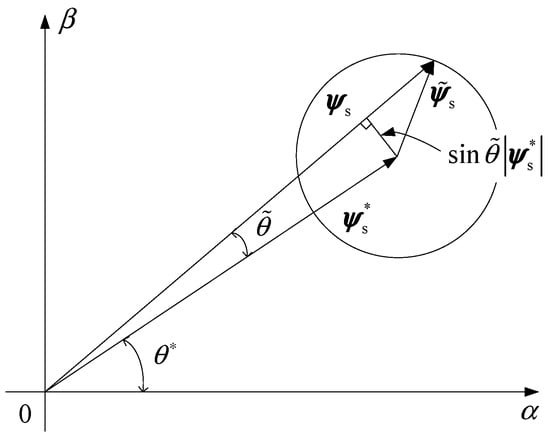
Figure 9.
The gain of nonlinear link .
At no load , for scalar , (where denotes a 2-norm, which is represents absolute value), resulting in
When , is the minimum, and , then start to increase at , equivalent to .
Nonlinear time-varying link, with as input
It passes through the center of the circle of the vector (when , ), and has
When , the value of begins to decrease, equal to 0.6366 at . When two links are connected in series, the gain of feedback link is in the range of
That is to say, the gain of the nonlinear system in the feedback path in Figure 9 is less than or equal to when is equal to 1, and then its maximum value begins to increase when the maximum value of is equal to 1.414.
The following is proof of the large-scale stability of the system shown in Figure 8, using the theory of passivity.
Figure 10 shows the process of calculating from for the nonlinear system in the feedback path of the system shown in Figure 8. From Figure 10, it can be seen that the angle between and is always less than or equal to (the figure shows , , and the same can be proved for other situations ), so
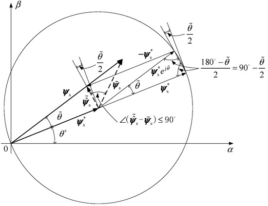
Figure 10.
Calculation of from .
That is, the feedback block of the system shown in Figure 10 is passive. According to the conclusion of system superstability, as long as the transfer function of the forward box is equal to
it is strictly true, and the system in Figure 10 is asymptotically stable (exponentially stable). The lower bound of the dot product . is given below. In , within the range of and also , so there is
in within range , so there is
That is to say, for a finite , the lower bound of the dot product tends to be zero because , so it cannot provide excessive passivity for the system.
2.2. When the Stator Current of the Motor Is Not Zero
In this portion, we will discuss the system’s stability when the motor stator current is not equal to zero (corresponding to the motor with external load or field weakening operation, hereafter referred to as external load). For the convenience of description, the system shown in Figure 1 is reconstructed in Figure 11. In the proposed method, there are four integral function blocks (I–IV), as shown in Figure 11. The first and second, namely I and II, are the integral blocks which are used for estimating the flux linkage observer, and the third and fourth, namely, the III and IV integral blocks, are the PLL speed and angle estimation integrals, respectively, which examine whether the system responses of the four integrators in Figure 11 converge together at different initial values.
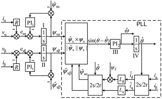
Figure 11.
Design of the flux observer with a PLL with external load.
The analysis method is the same as before, assuming
This is the steady-state solution of the system in Figure 11. Similarly, the system cannot be globally asymptotically stable because it has multiple equilibrium points. We will take the case of origin as an example.
Defining error signal
According to Figure 11, the corresponding equations are presented below
where
Henceforth,
Similarly,
Obviously, for the SPMSM () let ; therefore, it is the same as the situation under no load.
That is, for the hidden pole motor, in the error model, only the rotor error angle is adopted.
For any feedback action, the same linearization model and large-signal error model exist near the static working point. The PMSM with load is the same as without load. Figure 11 shows that the system is asymptotically stable. The above characteristics are very important for the application of the flux observer with a phase-locked loop in the asynchronous motor. At this time, the substitution inductance matrix L is a first-order inertial dynamic system with equal diagonal elements, and the static gain is equal to the mutual inductance among the stator and rotor of the motor, and the time constant is equal to the rotor’s time constant.
For salient pole motors, , hence
Thus, there is the small-signal model shown in Figure 12. It can be seen that under load conditions, unless , the conclusion that the linearized small-signal model is stable cannot be obtained by this method when the stator current of the motor is equal to zero.
Figure 12.
Small-signal model of the system with external load operation.
For the IPMSM , to discuss the stability of the large signal system in Figure 11, it is the same as that of no-load; it is considered that the frequency band of PLL is wide enough; therefore, we replace it with unity gain because
The above equations are represented in the system block diagram shown in Figure 13.
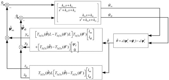
Figure 13.
The approximate system of Figure 11 when the dynamic of PLL is ignored.
Obviously, for a given stator current and , the static nonlinear systems of the two feedback branches are finite gains and cross the origin. Among them, the operation relationship of the nonlinear branch from to
The operational relationship with the first section
is the same, as shown in Figure 10; therefore,
and it is passive. However, the nonlinear branch from to , although it has finite gain and passes through the origin, is not passive. Next, the loop transformation method is used to compensate for the feedback path’s insufficient passivity by using the forward path’s excessive passivity.
For to , the nonlinear branches of the system are
In the above formula,
Use the Taylor series to expand around = 0, ignoring the second-order infinitesimal , and get
Therefore, for small-angle estimation errors, the following equation is used
In this way, when substituting . Let
Among these, the rotation transformations , are orthogonal matrices, and orthogonal transformation does not change the length of the vector, so the calculation of the induced norm of the matrix is as follows (suppose )
Therefore, there is
In this way, if the forward path transfer function in Figure 13 exhibits excessive passive k > 0, the loop transformation method is applied, as shown in Figure 14. Its stability is equivalent to that of the system shown in Figure 13 and the forward path transfer function of the system in Figure 14.
is strictly true, and the feedback path shows
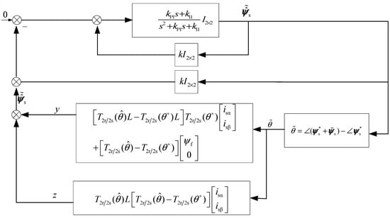
Figure 14.
Application of the loop transformation method to prove the stability of the system in Figure 11.
From the above results, when , take
When , the feedback path is also passive. Therefore, the system of Figure 11 is asymptotically stable near the equilibrium point when the relation is satisfied in non-heavy loads and deep weak magnetic fields. For a closed-loop transfer function composed of a PI regulator and an integrator
the condition of strictly true, as , , , namely . In this way, it can be deduced that the above transfer function is not too passive when , i.e., the maximum positive feedback coefficient is k = 0, which keeps the closed-loop transfer function strictly positive real, and when , the maximum positive feedback coefficient k = 1 keeps the closed-loop transfer function strictly positive real as shown in Appendix B.
The following content explains the stability region mentioned in the above results.
The matrix in formula () is
Its norm satisfies the relation
The characteristic equation of the matrix in the radical on the right side of the last equal sign in the above formula is
Its two characteristic roots are
Assume , then
When , , it is consistent with the results of the previous small-signal model.
The above results demonstrate that the flux observer design with PLL is unsuitable for the reluctance motor because the inductance of the two axes of the reluctance motor is not equal, and the flux value of a motor is equivalent to the product of the stator current times the inductance.
3. Simulation Results and Analysis
The velocity regulation system and block diagram of motion-sensorless control based on the proposed method is depicted in Figure 15 and Figure 16 respectively. The FOC, or vector control, is utilized as the primary control scheme. Based on a fundamental model, Figure 15 depicts an overall block diagram of a vector-controlled electrical motor drive with motion sensorless control. A sampled voltage and current are initially executed in the Clarke transformation to obtain the fixed reference frame voltage and current. The proposed method then provides the estimated rotor speed and position angle. The projected speed is sent back to the speed control loop, while the estimated position angle is employed to execute a rotating reference frame and inverse DQ transformation. This article proposes an improved switching method that utilizes an S-type function as a switching function to achieve a smooth state transition.
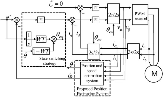
Figure 15.
A schematic representation of a proposed motion-sensorless velocity regulation system.
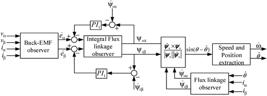
Figure 16.
A proposed motion-sensorless speed and position estimation block diagram.
The amplitude of torque current, an S-type function, is used as the weight function during the angle-switching process. Select an S-type function:
Among them is the given angular frequency of the motor, is the corresponding angular frequency when the weight changes to 0.5, and is a constant that can adjust the rate of change of the weight function. The variation curve of the weight function with angular frequency is shown in Figure 17.
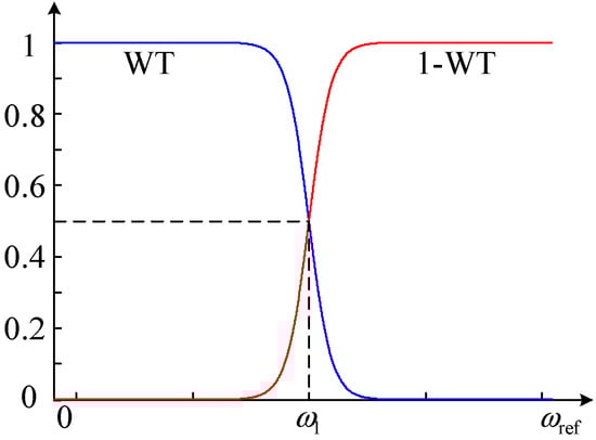
Figure 17.
S-type weight function variation curve.
The simulated interior PMSM parameters are shown in Table 1. Observer gains are shown in Table 2. Simulation/Simulink studies are conducted in this section to evaluate the performance of the new proposed rotor position angle estimator.

Table 1.
The specifications for the IPMSM used in the Simulink simulation and the experiment.
Table 2.
Observer gains.
A. Verification of Dynamic tracking performance
To verify the effectiveness of the proposed sensorless control algorithm and state-switching strategy, a model was built using MATLAB/Simulink for simulation verification. Figure 18 illustrates the performance of the proposed scheme under speed command variations.
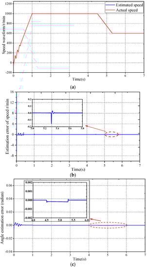
Figure 18.
Simulation results of the wide speed-range sensorless control system: (a) machine speedwaveform; (b) speed estimation deviation waveform; (c) rotor position estimation deviation.
Simulation setup: A ramp with a slope of 1000 r/min/s is set for the speed at 0–1 s. The speed increases from 0 r/min to 1000 r/min, and the speed is constant from 1–4.5 s. The command speed is reduced from 1000 r/min to 600 r/min at a rate of −1000 r/min/s at 4.5–5.5 s, and the speed is constant at 5.5–7 s; the motor is loaded with 10 Nm, and the initial given torque current is 20.51 A.
Figure 18a,b show that the speed estimated by the method proposed in this article can accurately track the actual value, with only a few speed estimation deviations below 400 r/min. After the state switch is completed, the speed estimation deviation is 0. The speed estimation deviation only exhibits a small deviation when the speed or torque current suddenly changes, which can be ignored. Figure 18c shows that in the first 0.4 s of the simulation, there is a certain deviation between the estimated and actual rotor positions. After the state switch is completed, the estimation deviation converges quickly. In the steady-state state, the estimation deviation of the rotor position is zero, and only a small deviation is caused by a phase-locked loop when the speed or torque current suddenly changes; overall, the simulation results show that the rotor position estimation method proposed in this paper can accurately estimate the position and speed of the rotor. Figure 19a shows that during the acceleration process, the torque current only fluctuates slightly when the speed loop is switched at 0.4 s, without significant fluctuation or oscillations. In the A-phase current curve shown in Figure 19b, there is no significant current mutation; from the speed waveform in Figure 18a, it can also be seen that there is no significant fluctuation in the speed during the state-switching process. The simulation results verify the feasibility and effectiveness of the proposed sensorless control method and state-switching strategy.
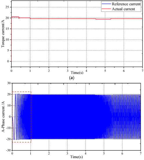
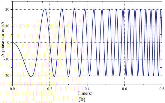
Figure 19.
Simulation results of the wide speed-range sensorless control system: (a) torque currentwaveform; (b) phase A current curve and its partially enlarged view.
B. Simulation results analysis of initial value
It is evident that the proposed design scheme in this article is a nonlinear system, and its stability is related to the type of input (the system in Figure 1 and Figure 11 is not asymptotically stable under any stator voltage or current input). To verify the asymptotic stability of the system in Figure 1 and Figure 11 under sinusoidal voltage and current inputs, it is only necessary to examine whether the system responses of the four integrators in the figure converge together at different initial values. Figure 20 shows the simulation results of the motor running at a constant speed of 30 rad/s with a load of 5 Nm. The system takes the sinusoidal voltage and current of the motor as inputs, and the integrators I, II, III, and IV give different initial values of 0.1 Wb, 0.05 Wb, 40 rad/s, 5.9 rad, and 0.09 Wb, 0.06 Wb, 20 rad/s, and 0.6 rad, respectively.
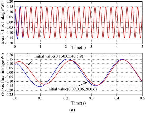
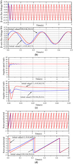
Figure 20.
System response under different initial values: (a) α-axis flux linkage; (b) β-axis flux linkage; (c) angular speed; (d) rotor position.
From the simulation results, it can be seen that under the condition of sinusoidal voltage and current input, and given different initial values of the four integrators, the outputs of the four integrators in the system shown in Figure 1 and Figure 11 can converge together, i.e., they can converge to the equilibrium state. From this, it can be seen that the design scheme shown in Figure 1 and Figure 11 is asymptotically stable under sinusoidal voltage and current inputs.
C. DC Disturbance Elimination
To further validate a proposed observer’s better DC elimination performance, results under DC disturbances are investigated, i.e., taking the -axis as an example. Figure 21 shows that no feedback is added when the stator back EMF contains a DC offset of 0.1 V. The PI regulators (), and coefficients are tuned to zero, while in the feedback function, the PI regulators (), and coefficients are adjusted to 100 and 200, respectively). However, when there is feedback, the gains of the PI regulator () can be selected in a wide range, and a good adjustment effect can be obtained. It is evident that when the stator flux linkage deviation feedback is not added, the flux linkage integral output shows a serious integral drift problem. After adding the feedback, the integral drift is well suppressed. Simulation comparison has verified that this method can effectively suppress the integral drift problem caused by DC bias.
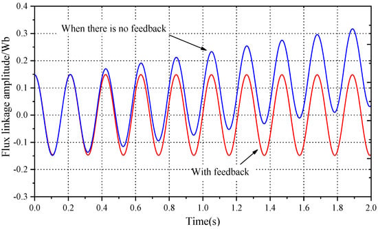
Figure 21.
Comparison between integral output, with and without feedback, under DC bias.
D. Verification of Robust Performance
The effectiveness of motion-sensorless control can be adversely affected, particularly in the low-speed region, by position errors caused by motor parameter variations. To verify the robustness of the motion sensorless control method proposed in the paper, the direct axis inductance is reduced by 20%, the permanent magnet flux linkage is increased by 5%, and the quadrature axis inductance parameter is reduced by 20%. All the simulation tests applying parameter mismatch are carried out at a constant speed of 80 rad/s with load torque 5 Nm. The simulation results are shown in Figure 22. It can be seen that under the condition of initial estimation bias when the system has no parameter error, the steady-state rotor position estimation bias can converge to 0; when there is an electrical parameter deviation in the system, there is a certain deviation in the estimated rotor position, but the system is still stable. In the proposed scheme, model parameters ,, and have a minimal effect on the angle error. The errors in result in a positional error but do not affect the system’s stability. Using the voltage and current of the motor loaded with 5 Nm, under variable speed operating conditions (as shown in Figure 23a) as input, simulation was conducted under the same parameter deviation. The simulation results are shown in Figure 23. Figure 2a shows the waveform of motor angular velocity variation. It operates at a constant speed of 80 rad/s at 0–1 s, increases from 80-rad/s to 100 rad/s at 1–1.05 s, then runs at a constant speed, decelerates from 100 rad/s to 80 rad/s at 2.95–2.98 s, and then runs at a constant speed. Figure 23b shows the scheme’s rotor position estimation deviation curve from Figure 1, with and without parameter errors. It can be seen from Figure 23b that the rotor position estimation deviation is 0 when there is no electrical parameter deviation. In the presence of electrical parameter deviations, the estimated deviation of the rotor position is −0.058 rad, when operating at a constant speed of 80 rad/s, and −0.043 rad, when operating at a constant speed of 100 rad/s, and it is also stable during acceleration and deceleration. The results of Figure 22 and Figure 23 illustrate the robust stability and performance of the scheme in Figure 1.
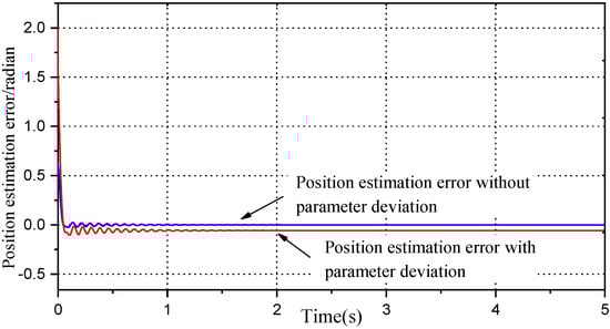
Figure 22.
Estimated position deviation with parameter deviation.
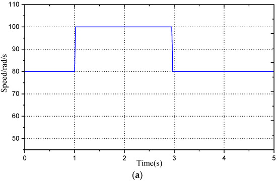
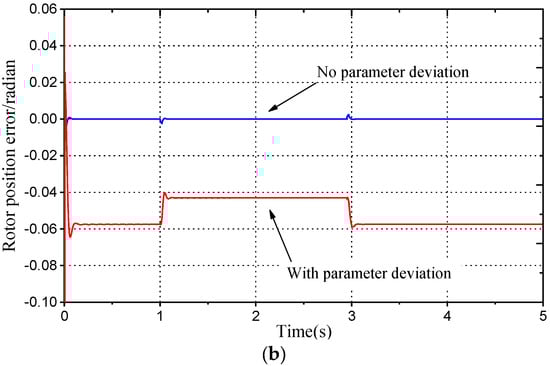
Figure 23.
Position estimation deviation under acceleration and deceleration conditions with parameter deviation: (a) angular velocity variation waveform; (b) rotor position deviation.
4. Experimental Results and Analysis
Using the Myway Company’s PE-expert4 platform, an experimental study of the proposed design observer’s operation was conducted. Power electronics and motor control systems are developed and experimented with on the PE-Expert4 platform as shown in the Figure 24. The platform uses Myway’s PE-View X integrated development environment in conjunction with T.I.’s high-speed floating point DSP (TMS320C6657) as its core, facilitating the development of a power converter and motor control system. A 14-bit A/D converter acquires the current signal, the PWM uses a 10 kHz carrier modulation output, and the motion-sensorless control strategy has a 100 µs control cycle. The stator voltage input of the rotor position estimation algorithm in the experiment is reconstructed from the motor command voltage, and the DC bus voltage is 200 V shown in the Figure 25. The rotor position is measured using the resolver. This position is not used for IPMSM speed control, but only for comparison with the estimated position.
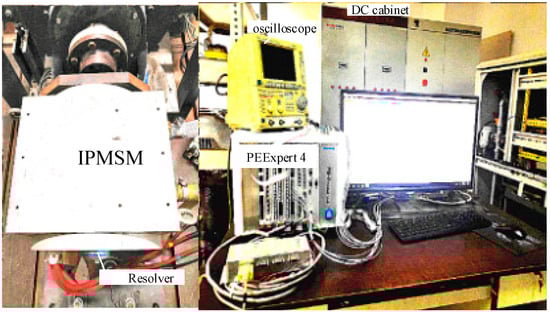
Figure 24.
Motor control system PE-Expert4.
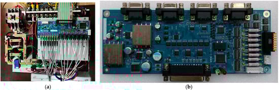
Figure 25.
Myway PE-expert4 experimental platform. (a) Inverter Unit MWINV-9R144; (b) MWACS-PSIF-01 Signal Conversion Board.
To validate whether the initial operations strategy can smoothly start the motor, in the experiment, the motor is initiated from a standstill and accelerated to a certain speed. In the experiment, the IF control method is initially used to accelerate the IPMSM motor from a speed of zero. The initial torque is specified as a current of 5 A, and the rotational speed is specified as a slope of 160 r/min/s. During state transitioning, the corresponding rotational speed is approximately 400 r/min and finally increases to 1000 r/min.
From Figure 26a, it is apparent that the estimated rotational speed can accurately follow the actual rotational speed, and when changing from the current closed-loop rotational speed open loop state to the current closed-loop rotational speed double closed-loop state, the rotational speed rises steadily in accordance with the reference value, without any abrupt changes or significant fluctuations, confirming the reliability of the rotational speed estimation method and the efficiency of the state switching method. Figure 26b shows the waveform of the actual position, estimated position, and estimated position deviation of the rotor, respectively, after the motor speed stabilizes. Figure 26b demonstrates that the estimated position follows the actual position accurately, and the estimated deviation is less than 0.07 rad, indicating the precision of the algorithm’s estimated position.
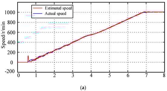
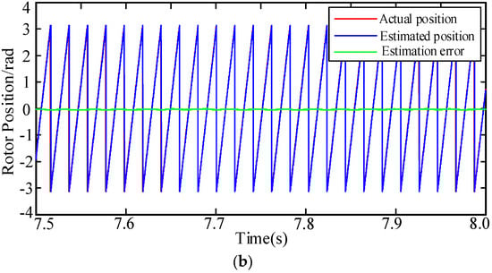
Figure 26.
Experimental results of motor starting strategy test: (a) motor speed tracking curve; (b) rotor position and position estimation deviation at steady state.
Figure 27 depicts the experimental results of the proposed observer dynamic performance under the rated load of the IPMSM, with a step change in rotational speed of 100–200 r/min. In the experiment, the motor was initially accelerated to 100 r/min and then maintained at a constant velocity. A dynamometer was used to apply a load of 15 Nm and provide a speed step command of 100–200 r/min at about 2.5 s.
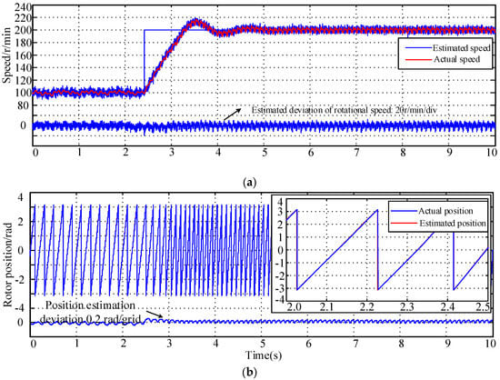
Figure 27.
Speed step test results under rated load: (a) motor speed and speed deviation waveform;(b) rotor position and rotor position estimation deviation waveform; (c) torque current waveform.
Figure 27a depicts the IPMSM reference rotational speed, real rotational speed, estimated rotational speed, and estimated rotational speed deviation curves. The figure demonstrates that the estimated rotational speed of the algorithm suggested in this article can always follow the actual rotational speed of the IPMSM, and the estimated rotational speed deviation is about 10 r/min in a steady state. When a given rotational speed step changes, an estimated deviation of only about 20 r/min occurs at a given time. During the process of increasing rotating speed, the estimated deviation of rotating speed is within 10 r/min for the majority of the time. Figure 27b depicts the waveforms of the real rotor position, estimated rotor position, and estimated rotor position deviation. The figure shows that the estimated rotor position value is nearly identical to the real value. In steady conditions, the average estimated rotor position deviation is about 0.015 rad, with a fluctuation amplitude of about 0.025 rad. When a given rotational speed step changes, the maximum estimated rotor position deviation does not surpass 0.07 rad. By increasing the integration coefficient in the phase-locked loop, error deviation can be reduced. The torque current trajectory is depicted in Figure 27c. The figure shows that the torque current is always around 40 A in a steady state, owing to a load of about 15 Nm. As the reference rotational speed is changed in steps, the torque current rapidly rises to around the amplitude limit of 50 A, causing the rotational speed to increase. Whenever the rotational speed reaches the desired magnitude, the torque current drops to around 40 A.
Although the proposed method is not applicable near zero speed, it may also have good operating characteristics at low speeds due to the compensation and DC bias suppression measures taken for inverter nonlinearity. To verify the lowest speed at which the method in this article can operate when the motor is under the rated load, the motor should be operated at low speed under the rated load. Through experimental testing, it was found that the algorithm in this paper can still achieve sensorless control of the motor at around 30 r/min with a load of 15 Nm. The estimated rotor position and speed are shown in Figure 28.
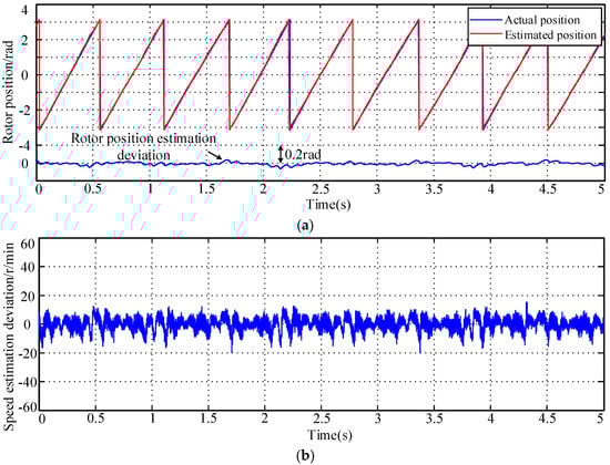
Figure 28.
Experimental results of motor operation under a rated load with 30 r/min: (a) rotor position and rotor position estimation deviation waveform; (b) speed estimation deviation waveform.
Figure 28 show that the rotor position estimation value proposed in this paper can still track the actual rotor position value when operating at 30 r/min with a rated load. The rotor position estimation deviation fluctuates around 0 rad, with a maximum estimation deviation of 0.06 rad. The speed estimation deviation fluctuates between 0–10 r/min. From the experimental results, it can be seen that under a rated condition, the estimated values of this method can accurately track the actual rotor position and speed, also exhibiting good dynamic estimation performance. Under a rated load, the motor can achieve sensorless operation at a low speed of 30 r/min. In summary, the position sensorless control method and state-switching strategy proposed in this article are feasible and effective.
5. Conclusions
The accurate rotor position angle estimation is essential to sensorless interior PMSM vector control. Its estimation accuracy will directly affect the operational effectiveness of the motor speed control system, especially its low-speed performance. A rotor angle and speed estimation technique based on the improved integrator using an adaptive compensation algorithm is proposed for the initial value problem and the DC bias problem of traditional back-EMF sensorless position detection of interior PMSM. An estimated value of a stator flux linkage has been obtained from the projected value of a rotor permanent magnetic flux linkage angle and the algebraic model (m-model) of a stator flux linkage, along with a synchronous coordinate system. An IPMSM sinusoidal stator flux linkage obtained from the stator current and integral voltage models in the static coordinate system is compared to form a feedback closed-loop to suppress the integral drift, and the estimated value of the IPMSM rotor speed and angle is achieved by using a cross product of the two through the phase-locked loop. An improved integrator flux observer is employed to remove the DC component, as well as high-order frequency harmonics, to minimize an angle error produced from current sampling and the converter’s nonlinearity. Compared to the traditional flux linkage observer, the proposed approach can eliminate the adverse effects of harmonics and the DC coefficient. The proposed method is relatively straightforward and can be used in a slow-speed area. The MATLAB/Simulink and experimental results demonstrate that the proposed model is robust for either rated or uncertain parameters. The proposed method can more precisely estimate the motor rotor angle in the broader speed range. Similarly, this technique is also applicable to the asynchronous motor. The possibility of implementing motion-sensorless control of a synchronous reluctance motor (SynRM) using the proposed technique will be further investigated.
Author Contributions
Conceptualization, C.X. and S.U.R.; methodology, C.X.; software, S.U.R.; validation, C.X. and S.U.R.; formal analysis, C.X.; investigation, S.U.R.; resources, C.X.; data curation, C.X.; writing—original draft preparation, C.X. and S.U.R.; writing—review and editing, C.X. and S.U.R.; visualization, C.X. and S.U.R.; supervision, C.X.; project administration, C.X.; funding acquisition, C.X. All authors have read and agreed to the published version of the manuscript.
Funding
This research received no external funding.
Data Availability Statement
All the data are shown in the tables and figures included in this paper.
Conflicts of Interest
The authors declare no conflict of interest.
Appendix A
When the stator current of the motor is equal to zero (no load condition) , according to Figure 1, the corresponding equations are presented below
where , and substituting into the Equation (A1) yields
Generally, if is the angle between the given vectors A and B, then the equation used for the vector cross product is:
Based on Equation (A2a), we can write Equation (A2b) as follows
Defining the error signal
Substituting Equation (A2c) into Equation (A2b), we get
The relationship between and is shown in Figure A1.

Figure A1.
A large-signal nonlinear model of a flux observer with a PLL.
Appendix B
For the PLL design in Figure A1, when the intersection angle between and is minimal, we get ; subsequently, the transfer function of the phase-locked loop near the equilibrium point is
and in Equation (A3) are the proportional gain and the integral gain. The estimation performance is determined solely by the PI gains of and . In this paper, the design proportion and integral coefficients are
The damping coefficient of the system , is the undamped oscillation frequency of the system, and is 1000 rad/s, based on the motor’s speed operating range. Because the open-loop transfer function of PLL has two integral links, is the ramp input for the step input of speed, which can achieve no static error, that is, in the steady-state; for the ramp input of speed, is a parabolic input with static error, and the size of the static error is inversely proportional to .
References
- Bolognani, S.; Oboe, R.; Zigliotto, M. Sensorless Full-Digital PMSM Drive with EKF Estimation of Speed and Rotor Position. IEEE Trans. Ind. Electron. 1999, 46, 184–191. [Google Scholar] [CrossRef]
- Solsona, J.; Valla, M.I.; Muravchik, C. Nonlinear Control of a Permanent Magnet Synchronous Motor with Disturbance Torque Estimation. IEEE Trans. Energy Convers. 2000, 15, 163–168. [Google Scholar] [CrossRef] [PubMed]
- Yao, Y.; Huang, Y.; Peng, F.; Dong, J. Position Sensorless Drive and Online Parameter Estimation for Surface-Mounted PMSMs Based on Adaptive Full-State Feedback Control. IEEE Trans. Power Electron. 2020, 35, 7341–7355. [Google Scholar] [CrossRef]
- Qiao, Z.; Shi, T.; Wang, Y.; Yan, Y.; Xia, C.; He, X. New Sliding-Mode Observer for Position Sensorless Control of Permanent-Magnet Synchronous Motor. IEEE Trans. Ind. Electron. 2013, 60, 710–719. [Google Scholar] [CrossRef]
- Li, Z.; Ao, N.; Wang, X. Position Sensorless Control of PMSM Based on a Sliding Mode Observer. J. Inst. Ind. Appl. Eng. 2016, 4, 33–39. [Google Scholar] [CrossRef]
- Lara, J.; Chandra, A. Performance Investigation of Two Novel HSFSI Demodulation Algorithms for Encoderless FOC of PMSMs Intended for E.V. Propulsion. IEEE Trans. Ind. Electron. 2018, 65, 1074–1083. [Google Scholar] [CrossRef]
- Chen, Z.; Tomita, M.; Doki, S.; Okuma, S. An Extended Electromotive Force Model for Sensorless Control of Interior Permanent-Magnet Synchronous Motors. IEEE Trans. Ind. Electron. 2003, 50, 288–295. [Google Scholar] [CrossRef]
- Xu, Z.; Rahman, M.F. Comparison of a Sliding Observer and a Kalman Filter for Direct-Torque-Controlled IPM Synchronous Motor Drives. IEEE Trans. Ind. Electron. 2012, 59, 4179–4188. [Google Scholar] [CrossRef]
- Liu, J.M.; Zhu, Z.Q. Novel Sensorless Control Strategy With Injection of High-Frequency Pulsating Carrier Signal Into Stationary Reference Frame. IEEE Trans. Ind. Appl. 2014, 50, 2574–2583. [Google Scholar] [CrossRef]
- Han, D.Y.; Cho, Y.; Lee, K.-B. Simple Sensorless Control of Interior Permanent Magnet Synchronous Motor Using PLL Based on Extended EMF. J. Electr. Eng. Technol. 2017, 12, 711–717. [Google Scholar] [CrossRef]
- Morimoto, S.; Kawamoto, K.; Sanada, M.; Takeda, Y. Sensorless Control Strategy for Salient-Pole PMSM Based on Extended EMF in Rotating Reference Frame. IEEE Trans. Ind. Appl. 2002, 38, 1054–1061. [Google Scholar] [CrossRef]
- Lee, J.; Hong, J.; Nam, K.; Ortega, R.; Praly, L.; Astolfi, A. Sensorless Control of Surface-Mount Permanent-Magnet Synchronous Motors Based on a Nonlinear Observer. IEEE Trans. Power Electron. 2010, 25, 290–297. [Google Scholar] [CrossRef]
- Choi, J.; Nam, K.; Bobtsov, A.A.; Pyrkin, A.; Ortega, R. Robust Adaptive Sensorless Control for Permanent-Magnet Synchronous Motors. IEEE Trans. Power Electron. 2017, 32, 3989–3997. [Google Scholar] [CrossRef]
- Feng, G.; Lai, C.; Mukherjee, K.; Kar, N.C. Online PMSM Magnet Flux-Linkage Estimation for Rotor Magnet Condition Monitoring Using Measured Speed Harmonics. IEEE Trans. Ind. Appl. 2017, 53, 2786–2794. [Google Scholar] [CrossRef]
- Bobtsov, A.A.; Pyrkin, A.A.; Ortega, R.; Vukosavic, S.N.; Stankovic, A.M.; Panteley, E.V. A Robust Globally Convergent Position Observer for the Permanent Magnet Synchronous Motor. Automatica 2015, 61, 47–54. [Google Scholar] [CrossRef]
- Ortega, R.; Praly, L.; Astolfi, A.; Lee, J.; Nam, K. Estimation of Rotor Position and Speed of Permanent Magnet Synchronous Motors With Guaranteed Stability. IEEE Trans. Control Syst. Technol. 2011, 19, 601–614. [Google Scholar] [CrossRef]
- Po-ngam, S.; Sangwongwanich, S. Stability and Dynamic Performance Improvement of Adaptive Full-Order Observers for Sensorless PMSM Drive. IEEE Trans. Power Electron. 2012, 27, 588–600. [Google Scholar] [CrossRef]
- Park, Y.; Sul, S.-K. Sensorless Control Method for PMSM Based on Frequency-Adaptive Disturbance Observer. IEEE J. Emerg. Sel. Top. Power Electron. 2014, 2, 143–151. [Google Scholar] [CrossRef]
- Bose, B.K.; Patel, N.R. A Programmable Cascaded Low-Pass Filter-Based Flux Synthesis for a Stator Flux-Oriented Vector-Controlled Induction Motor Drive. IEEE Trans. Ind. Electron. 1997, 44, 140–143. [Google Scholar] [CrossRef]
- Song, J.; Niu, Y.; Zou, Y. Asynchronous Sliding Mode Control of Markovian Jump Systems with Time-Varying Delays and Partly Accessible Mode Detection Probabilities. Automatica 2018, 93, 33–41. [Google Scholar] [CrossRef]
- Boussekra, F.; Makouf, A. Sensorless Speed Control of IPMSM Using Sliding Mode Observer Based on Active Flux Concept. Model. Meas. Control A 2020, 93, 1–9. [Google Scholar] [CrossRef]
- Chen, S.; Zhang, X.; Wu, X.; Tan, G.; Chen, X. Sensorless Control for IPMSM Based on Adaptive Super-Twisting Sliding-Mode Observer and Improved Phase-Locked Loop. Energies 2019, 12, 1225. [Google Scholar] [CrossRef]
- Piippo, A.; Hinkkanen, M.; Luomi, J. Analysis of an Adaptive Observer for Sensorless Control of Interior Permanent Magnet Synchronous Motors. IEEE Trans. Ind. Electron. 2008, 55, 570–576. [Google Scholar] [CrossRef]
- Piippo, A.; Hinkkanen, M.; Luomi, J. Adaptation of Motor Parameters in Sensorless PMSM Drives. IEEE Trans. Ind. Appl. 2009, 45, 203–212. [Google Scholar] [CrossRef]
- Hinkkanen, M.; Tuovinen, T.; Harnefors, L.; Luomi, J. A Combined Position and Stator-Resistance Observer for Salient PMSM Drives: Design and Stability Analysis. IEEE Trans. Power Electron. 2012, 27, 601–609. [Google Scholar] [CrossRef]
- Jiang, Y.; Xu, W.; Mu, C. Improved SOIFO-based rotor flux observer for PMSM sensorless control. In Proceedings of the IECON 2017—43rd Annual Conference of the IEEE Industrial Electronics Society, Beijing, China, 29 October–1 November 2017; pp. 8219–8224. [Google Scholar]
- Xu, W.; Jiang, Y.; Mu, C.; Blaabjerg, F. Improved Nonlinear Flux Observer-Based Second-Order SOIFO for PMSM Sensorless Control. IEEE Trans. Power Electron. 2019, 34, 565–579. [Google Scholar] [CrossRef]
- Xu, W.; Wang, L.; Liu, Y.; Blaabjerg, F. Improved Rotor Flux Observer for Sensorless Control of PMSM with Adaptive Harmonic Elimination and Phase Compensation. CES Trans. Electr. Mach. Syst. 2019, 3, 151–159. [Google Scholar] [CrossRef]
- Lascu, C.; Andreescu, G.-D. PLL Position and Speed Observer With Integrated Current Observer for Sensorless PMSM Drives. IEEE Trans. Ind. Electron. 2020, 67, 5990–5999. [Google Scholar] [CrossRef]
- Lee, S.-J.; Kim, T.-W.; Kim, W.-S.; Kim, M.-G.; Jung, Y.-S. Performance Improvement of Sensorless Control of IPMSM Using Active Flux Concept by Improved Current Estimators. Trans. Korean Inst. Power Electron. 2013, 18, 587–592. [Google Scholar] [CrossRef]
- Foo, G.; Rahman, M.F. Sensorless Vector Control of Interior Permanent Magnet Synchronous Motor Drives at Very Low Speed without Signal Injection. IET Electr. Power Appl. 2010, 4, 131. [Google Scholar] [CrossRef]
Disclaimer/Publisher’s Note: The statements, opinions and data contained in all publications are solely those of the individual author(s) and contributor(s) and not of MDPI and/or the editor(s). MDPI and/or the editor(s) disclaim responsibility for any injury to people or property resulting from any ideas, methods, instructions or products referred to in the content. |
© 2023 by the authors. Licensee MDPI, Basel, Switzerland. This article is an open access article distributed under the terms and conditions of the Creative Commons Attribution (CC BY) license (https://creativecommons.org/licenses/by/4.0/).