Fault Detection, Diagnostics, and Treatment in Automated Manufacturing Systems Using Internet of Things and Colored Petri Nets

Abstract

Internet of things (IoT) applications, which include environmental sensors and control of automated manufacturing systems (AMS), are growing at a rapid rate. In terms of hardware and software designs, communication protocols, and/or manufacturers, IoT devices can be extremely heterogeneous. Therefore, when these devices are interconnected to create a complicated system, it can be very difficult to detect and fix any failures. This paper proposes a new reliability design methodology using “colored resource-oriented Petri nets” (CROPNs) and IoT to identify significant reliability metrics in AMS, which can assist in accurate diagnosis, prognosis, and resulting automated repair to enhance the adaptability of IoT devices within complicated cyber-physical systems (CPSs). First, a CROPN is constructed to state “sufficient and necessary conditions” for the liveness of the CROPN under resource failures and deadlocks. Then, a “fault diagnosis and treatment” technique is presented, which combines the resulting network with IoT to guarantee the reliability of the CROPN. In addition, a GPenSIM tool is used to verify, validate, and analyze the reliability of the IoT-based CROPN. Comparing the results to those found in the literature shows that they are structurally simpler and more effective in solving the deadlock issue and modeling AMS reliability.

1. Introduction

The growth of the “internet of things” (IoT) and “information and communications technology” (ICT) [1] has made it possible for “cyber-physical systems” [2] to be used to control and manage AMS. The IoT is a set of real objects equipped with “sensors”, “software”, and other ICT systems that enable them to interact with other systems and devices over the internet. ICT, on the other hand, is any type of “computing/communication” equipment, “networking devices”, and “information systems” that make it easier to interact in the digital world. The IoT is an essential component of the next generation of information methods; it is the internet that connects physical objects, which in turn connect the internet with the real world. In accordance with the agreement, physical objects are linked to the internet for information communication and exchange via “radio frequency identification” (RFID), “sensors”, and a few other tools. Therefore, things can be intelligently identified, located, and controlled [3].

Cyber-physical systems (CPS) integrate sensor networks and embedded computing to control and monitor the physical environment in the context of manufacturing systems, including control loops that enable environmental stimuli to activate the control, communication, or computing automatically [4]. The development of the IoT and ICT provides the capability to control, monitor, and manage CPS via the prompt delivery of real-time data from the manufacturing system. In CPS of manufacturing systems, machine/resource failures are common. Managers are frequently concerned with whether the planned due dates of orders can be achieved if machines fail, i.e., if the AMS is robust against failures. Even though IoT and ICT can detect real-time information in CPS, including “resource failures”, poor response to “resource failures” can damage CPS and reduce performance. The CPS can only be robust when the real-time data presented by “IoT” and “ICT” is employed to enhance decision-making and adapt to a dynamic environment in a timely way. Information from IoT and ICT about “resource failures” in real time is only relevant if an efficient system exists to assess and analyze the impacts of “resource malfunctions” and deal with them [3]. Therefore, the CPS requires a strategy to evaluate the effects of “resource failures”, support decision-making, and take the necessary actions in response to “resource failures”. This motivates us to design a technique to evaluate the effects of “resource failures” on CPS operations and provide the necessary decision support.

Several manufacturers have concentrated their efforts on improving the effectiveness of computer numerical control (CNC) machine tools with high accuracy and superior surface quality. In CNC machines, managing frequent failures, such as “tool wear”, “noise”, and “tool breakage”, is a problem. Tool wear is a complex process to control because it is not a linear operation; tools degrade quickly at first, then at a reasonable rate for a duration of time, and finally at an increasing rate until complete failure. Tool wear is a common and unavoidable problem during most machining processes. It presents a variety of obstacles to the quality and productivity of automated machining operations, impeding the possibility of intelligent and integrated industrial companies [5].

Nowadays, the construction of an intelligent online method for condition monitoring based on industrial IoT for manufacturing systems has become a solution for advanced predictive maintenance systems that continuously monitor and record the status of CNC machine tools [6].

Recently, effective fault diagnosis and detection approaches based on IoT, CPS, and artificial machine learning have been developed. The authors of [7] developed a new IoT architecture for online monitoring of induction motor faults. The developed IoT architecture recognizes the fault categories of the motor using effective machine learning methods. In addition, cyber-attacks are considered, and the proposed IoT architecture can detect and avoid cyber-attacks. The results highlight the advantages of the proposed IoT infrastructure to accurately identify motor faults and cyberattacks. The authors of [8] proposed a new smart IoT system for vibration monitoring and control of the milling CNC machine center. The milling machine was connected to a force sensor to record the vibrations caused by the cutting process. The IoT system employing the “message queue telemetry transport” (MQTT) protocol was built to connect the sensor node to the cloud server in order to record the cutting conditions. Deep learning neural networks are used to classify cutting states such as “stable cutting”, “unstable cutting”, and “fake cutting”. Moreover, if there is a cyberattack, the proposed method can switch the IoT system automatically to the backup broker to keep cutting operations safe and reliable. The authors of [9] developed and prototyped an “event-driven tool condition monitoring” (EDTCM) system that is activated “just in time” after the workpiece begins processing. The authors of [10] proposed a flexible and simple tool condition monitoring system in which the algorithms use repetitive machining processes in mass production and employ similarity analysis between the data of known conditions and received signals. The authors of [11] reviewed and evaluated direct and indirect sensing approaches for tool condition monitoring in milling, and discussed the strengths, drawbacks, and future prospects of such measurement techniques. The authors of [12] conducted research on energy harvesting systems for “wireless sensor nodes” (WSNs), directly addressing the issue of wireless sensor batteries’ sustainability.

The authors of [13] presented a practical lightweight model EPN and a definition “language EPNML” based on Petri nets (PNs) to represent the IoT services’ behavior and business processes, such as process control and logic relationship architecture. To improve the efficiency and adaptability of IoT services, this model was developed. The authors of [14] modeled the connection between different sensors and the “geographic environment” by employing “colored Petri nets” (CPNs). As data and processing services, they categorize the “IoT service”, the “geographic entity”, and the “Geographic Information System” (GIS) service. In order to do this, CPNs and an algebra were used to represent and evaluate “geo characteristics”, “IoT”, and “Geographic Information System” services, and the connection activity between a “sensor” node and its “geographic environment”. Using three different case studies, they illustrated the validity of the CPN-based assessment method. The authors of [15] presented a CPN technique to represent the global behavior of “wireless sensor networks”, which contains the energy usage of the network. CPNs and the principle of “component-oriented modeling” form the basis of their method. Two components are highlighted: the “radio system” and the “MAC Protocol”. Models for each subnet and interface were then developed separately. The study evaluated the network based on its energy usage, allowing them to estimate its life. In [16], CPNs were used to represent the “1-wire protocol” that is employed to connect a master device with many small, inexpensive devices, including “digital thermometers” and “weather sensors”, throughout a single shared bus with “low data rates” and “large ranges”.

As aforementioned in the literature, manufacturers use careful operational technology to avoid these failures in order to avoid costly tool wear and damage [17]. This, unfortunately, leads to less productive and costly operations due to the requirement to replace the tool early, the downtime of a machine, and replacement costs. To solve this problem, manufacturers can apply sensors to monitor tool conditions and manage the system in real time. These sensors include acoustic emission sensors [18], accelerometers and current sensors [19]. Because a single sensor cannot accurately determine the status of a tool under varying operational conditions, combining the data from multiple sensors can be the main obstacle. Using information that is partially redundant, this data acquisition can provide decision-making information for a process with less uncertainty. Earlier solutions attempted to derive a tool’s status from data by extracting relevant characteristics. Therefore, this study aims to propose a “colored resource-oriented Petri nets” (CROPNs)-based IoT for sensor systems in order to detect and remedy failures. Using the main CROPN properties, we are able to construct a system with a huge number of sensors. The study’s purpose is to present a technique for modeling reliability, based on CROPN and IoT, to identify critical reliability measures in AMS, including “mean time to failure”, “mean time to repair”, and “availability”. First, a CROPN that considers “resource failures” is designed to guarantee the liveness of the CROPN. Then, a method is developed for “fault detection and treatment” that integrates IoT and CROPN to ensure the system’s reliability. Moreover, the system’s reliability is evaluated using CROPN and IoT. The following is a list of the significant contributions of the study:

(1)

The development of a new approach for modeling the reliability and deadlock control of complicated AMS.

(2)

The IoT-based CROPN is used to present tool-wear monitoring on a milling machine as an example of an actual system that is generally difficult to model, evaluate performance, and monitor tool status on various machines.

(3)

The GPenSIM tool [20,21,22,23,24] is used to propose a comprehensive simulation program for the IoT-based CROPN that is then employed to simulate, verify, and evaluate results.

The rest of this paper is structured as follows: Section 2 shows the development of the CROPN and its “deadlock avoidance” strategy. The CROPN and IoT combination for “fault detection and treatment” and the reliability model are illustrated in Section 3. In Section 4, we present the actual AMS example that demonstrates the experimental outcomes of the designed methodology. In Section 5, the developed CROPN based on the IoT is validated and compared to other existing approaches. Conclusions and research directions are presented in Section 6.

2. Synthesis Method of CROPN

Based on its stated processing paths, a ROPN defines a component production process as a component sequentially visiting the resources. ROPN expresses machines and buffers as H-resources [25,26,27,28] of the same resource type. Each resource is created in a single location. The paths a product travels to obtain its resources define its production processes. If each component’s production process is constructed in an efficient manner, the model is highly compressed and demonstrates a number of important structural characteristics. Moreover, the ROPN considers material handling equipment to be a special type of resource, known as G-resources [25,26,27,28]. Due to the restricted resources available in the production system, a limited capacity PN with its related firing rules is employed. A transition in a ROPN indicates the movement of a part from one resource to another. The AMS can be modeled by the ROPN in two steps: (1) designing the component manufacturing process regardless of component transportation, and (2) designing the component handling operations using the model constructed in step 1.

A CROPN can be expressed by N = (P, T, C, I, O, K, M), where

(1)

P = {p_o} ∪ {p_r} ∪ P_R is a number of model places, where p_o is a load/unload idle place, p_r is a global place that represents material handling equipment resources, and P_R = ∪_i∈m{p_i}, represents a set of model resource places, m > 0;

(2)

T = ∪_j∈n{t_j} represents a number of model transitions, where n > 0, P ∩ T = φ, and P ∪ T ≠ φ;

(3)

C(p) and C(t) are, respectively, the sets of color related to CROPN places and transitions, where

(4)

∀p_i ∈ P, C(p_i) = ∪_i∈m{a_iu}, u = |C(p_i)|

(5)

∀t_j ∈ T, C(t_j) = ∪_j∈n{b_jv}, v = |C(t_j)|;

(6)

I(p, t): C(p) × C(t) →IN represents the function of the input of the CROPN, and IN = {0, 1, 2,...};

(7)

O(p, t): C(p) × C(t) →IN represents the function of the output of the CROPN;

(8)

K: P →IN denotes the capacity function, which allocates the maximum tokens for each p_i ∈ P and is represented as K(p_i);

(9)

M: P → N indicates the function of the CROPN state (marking) that adds tokens to each place in a CROPN. M(p_i) represents the tokens in place p_i regardless of its color. M(p_i, a_ij) represents the tokens in place p_i with color a_ij. M_o denotes the initial state of the CROPN.

Assuming that F= I(p_i, t_j) ∪ O(p_i, t_j), ∀(p_i, t_j) ∈ F, the preset (input) and postset (output) transitions of place p_i can be expressed as “^•p_i = {t_j ∈ T | (t_j, p_i) ∈ F}” and “p_i^• = {t_j ∈ T | (p_i, t_j) ∈ F}”, respectively. Similarly, the preset (input) and postset (output) places of transition t_j can be, respectively, expressed as “^•t_j = {p_i ∈ P | (p_i, t_j) ∈ F}” and “ t_j^• = {p_i ∈ P | (t_j, p_i) ∈ F}”. A CROPN can be called

(1)

ordinary when “I(p_i, t_j)(a_ih, b_jk) = 1”, ∀(p_i, t_j) ∈ F, p_i ∈ P, t_j ∈ T;

(2)

weighted when “I(p_i, t_j)(a_ih, b_jk) > 1”, (p_i, t_j) ∈ F, ∃p_i ∈ P, and ∃t_j ∈ T;

(3)

self-loop-free when “I(p_i, t_j)(a_ih, b_jk) > 0”, “O(p_i, t_j)(a_ih, b_jk)= 0”, and ∀(p_i, t_j) ∈ P ∪ T;

(4)

self-loop when “I(p_i, t_j)(a_ih, b_jk) > 0”, “O(p_i, t_j)(a_ih, b_jk) > 0”, and ∀(p_i, t_j) ∈ P ∪ T.

In a CROPN, a t_j ∈ T is “process-resource-enabled” [28] if

“M(p_i, a_ih) ≥ I(p_i, t_j)(a_ih, b_jk), ∀p_i ∈ P, ∀p_i ∈ ^•t_j, a_ih ∈ C(p_i), b_ik ∈ C(t_j),”

(1)

and

“K(p_i) ≥ M(p_i, a_ih) + O(p_i, t_j)(a_ih, b_jk) − I(p_i, t_j)(a_ih, b_jk), ∀p_i ∈ P, ∀p_i ∈ t_j^•, a_ih ∈ C(p_i), b_ik ∈ C(t_j).”

(2)

At state M, if a transition t_j ∈ T is enabled, it fires, and the state changes from M to M’, denoted as M[t_j⟩M′ and stated as

“∀p_i ∈ P, a_ih ∈ C(p_i), b_ik ∈ C(t_j), M′(p_i, a_ih) = M(p_i, a_ih) + O(p_i, t_j)(a_ih, b_jk) − I(p_i, t_j)(a_ih, b_jk).”

(3)

A CROPN has multiple circuits due to its high connectivity. Production process circuits (PPCs) are unique circuits in a CROPN that play a significant influence in its liveness. There are no idle places in PPCs, which are denoted as PPCs = {e₁, e₂, …, e_r}, r > 0, where e_r is a circuit in PPCs. When an e_r flows from a node a to multiple nodes and then back to the originating node a without duplicating any nodes, it said to be an elementary circuit. An e_r is non-elementary if it does not return to the initial node a. Moreover, in the e_r, the sets transitions must equal the sets of places, such that “|P(e_r)| = |T(e_r)|”, where P(e_r) represents the number of places in the e_r and T(e_r) denotes the number of transitions in the e_r, respectively, and the input places of transition t_j for an e_r “(^•t_j∈ P(e_r), p_i ∈ ^•t_j)” must be included in the e_r. If the t_j in a circuit e_r fires and the tokens leave the e_r, the tokens are described as the “departing tokens” and the “cycling tokens” when they do not leave a circuit e_r, and can be formulated as

p_i ∈ P(e_r), M(e_r) = ΣM(p_i, e_r)

(4)

where M(p_i, e_r) indicates the number of tokens in p_i, which enables t_j in an e_r.

It is said that a circuit e_r^c is an interactive subnet, which contains c PPCs, c > 0, if its transitions and places are shared with at least one other PPC and its connections are strong. If a transition t_j in e_r^c (p_i ∈ P(e_r^c) and t_j^•∈ (p_i^•∩ T(e_r^c))) fires and the tokens leave the e_r^c, where P(e_r^c) represents the set of places and T(e_r^c) denotes the set of transitions in an e_r^c, the tokens in e_r^c are known as the “departing tokens”; otherwise, they are said to be the “cycling tokens”, and can be stated as

p_i ∈ P(e_r^c), M(e_r^c) = ΣM(p_i, e_r^c)

(5)

where M(p_i, e_r^c) denotes the number of tokens in p_i, which enables t_j in an e_r^c.

In a CROPN,

(1)

if the t_j satisfies conditions in Equations (1) and (2), it said to be a controlled transition;

(2)

if there is at least one controlled transition t_j, then the CROPN is called a controlled net;

(3)

if a circuit e_r satisfies the conditions in Equations (1) and (2), then it is said to be enabled;

(4)

if the t_j ∈ T(e_r) is live (deadlock-free), the t_j is called live;

(5)

the t_j is called an input and output transition of an e_r^c if the t_j ⊄ T(e_r^c), t_j^• ∈ P(e_r^c), and ^•t_j ∈ P(e_r^c).

The following are the conditions necessary for a deadlock-free CROPN:

1.

Condition 1 [28]: A CROPN is not deadlock-free if

“M_o(p_o) ≥ K(e_r).”

(6)

2.

Condition 2 [28]: At any state M ∈ R(N, M_o), a circuit e_r is live if

“S′(e_r) ≥ 1,”

(7)

where R(N, M_o) represents the CROPN reachable states, and S′(e_r) is the current number of spaces in an e_r, and can be expressed as

“S′(e_r) =K(e_r) − M(e_r).”

(8)

3.

Condition 3: At any state M ∈ R(N, M_o), when Condition 2 is satisfied, transitions in T(e_r) and T_I(e_r) are controlled, where T_I(e_r) represents the set of input transitions in an e_r (see DFC-Policy in [29]);

4.

Condition 4 [28]: At any state M ∈ R(N, M_o), a circuit e_r^c is deadlock-free if

“S′(e_r) ≥ 1,” ∀e_r

(9)

and

“η(e_r^c, M) ≥ 1,”

(10)

where η(e_r^c, M) denotes the enabled PPCs in an e_r^c

5.

Condition 5 [28]: At any marking M, an e_r^c is deadlock-free if

(a)

any t_j ∈ T_I(e_r^c) is controlled, where T_I(e_r^c) denotes the set of input transitions in the e_r^c;

(b)

before a controlled t_j fires, each e_r ∈ V_en(t_j), S′(e_r) ≥ 2, where V_en(t_j) represents the set of PPCs in the CROPN and the t_j denotes the input transition of these PPCs;

(c)

the state M can be modified to M’ after the firing of the t_j, such that “η(e_r^c, M) ≥ 1”.

6.

Condition 6 [28]: If a CROPN has no PPC, then it is always live.

Based on the above conditions, Algorithm 1 shows the deadlock avoidance algorithm for a CROPN model.

Algorithm 1Policy for avoiding deadlock in the CROPN.

Input:TheCROPN model; Output:The controlled CROPNmodel; Compute PPCs = {e1,e2, …, er}, r > 0 of the CROPN model; Compute all reachable markings R (N, Mo) of the CROPN model; ifthe PPCs ≠φ, then  for (1 ≤ | PPCs | ≤ r++), do   if an er is not an interactive and p ∈ P(er), then       for (0 ≤ | R (N, Mo)| ≤ k++), do         K(er) = ΣK(p, er);         Mk(er) = ΣMw(p, er);         S′(er) =K(er) − Mk(er);         if S′(er) ≥1, then           The er has no deadlock states;         else if           The er has deadlock states;           Implement the DFC-Policy in [29] to avoid deadlock states;       end for  else if an er is an interactive and p ∈ P(er), then       for (0 ≤ | R (N, Mo)| ≤ j++) do         K(er) = ΣK(p, er);         Mk(er) = ΣMj(p, er);         S′(er) =K(er) − Mj(er);         if S′(er) ≥ 1 and η(erc, Mj) ≥1, then           The er has no deadlock states;         else if           The er has deadlock states;           Implement the condition 5 to avoid deadlock states;       end for   end if  end for else if The er is deadlock-free based on condition 6; end if Output:A controlled CROPN model End

3. Hybrid CROPNs and IoT

3.1. CROPN Synthesis Based on IoT

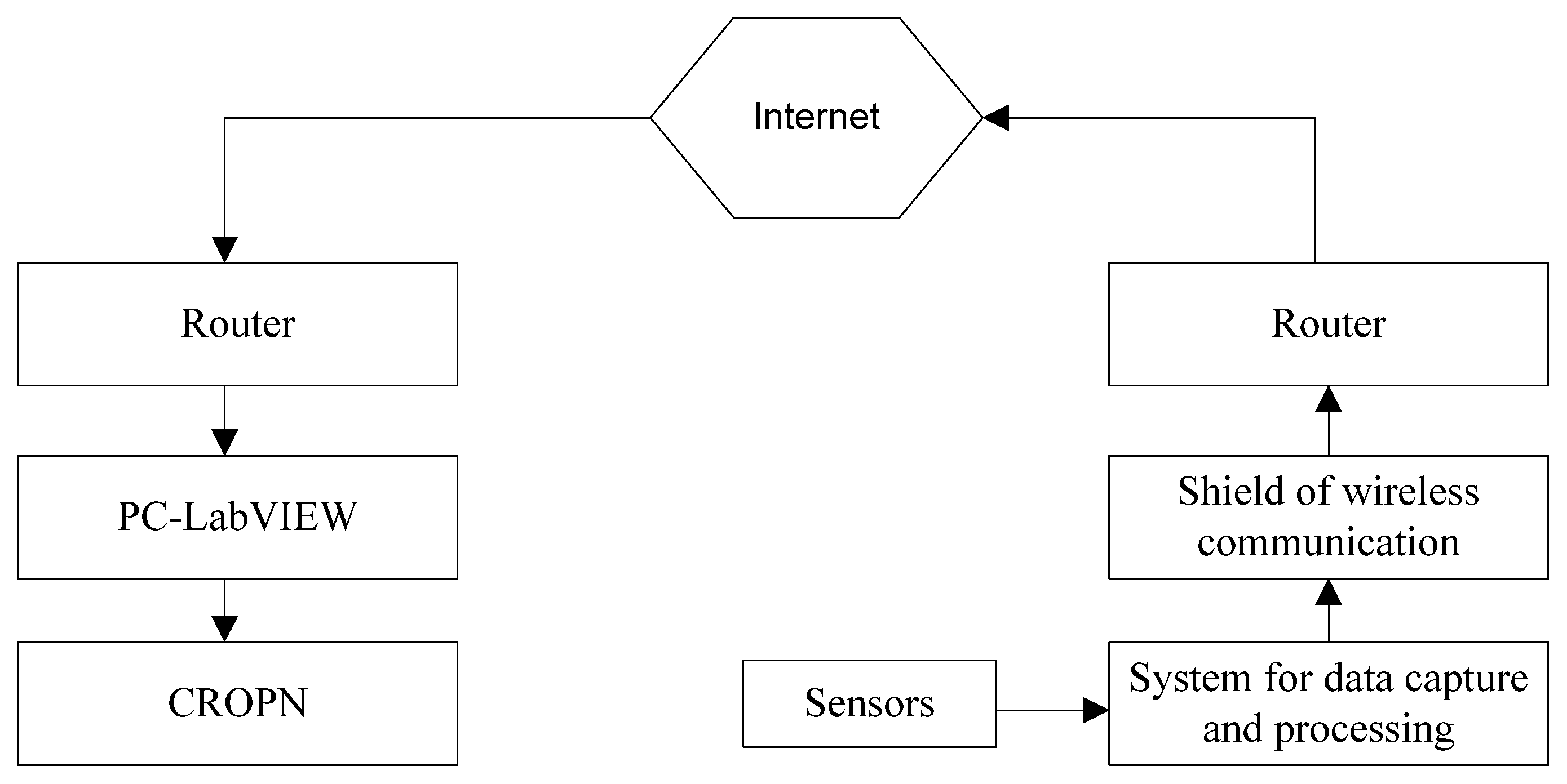
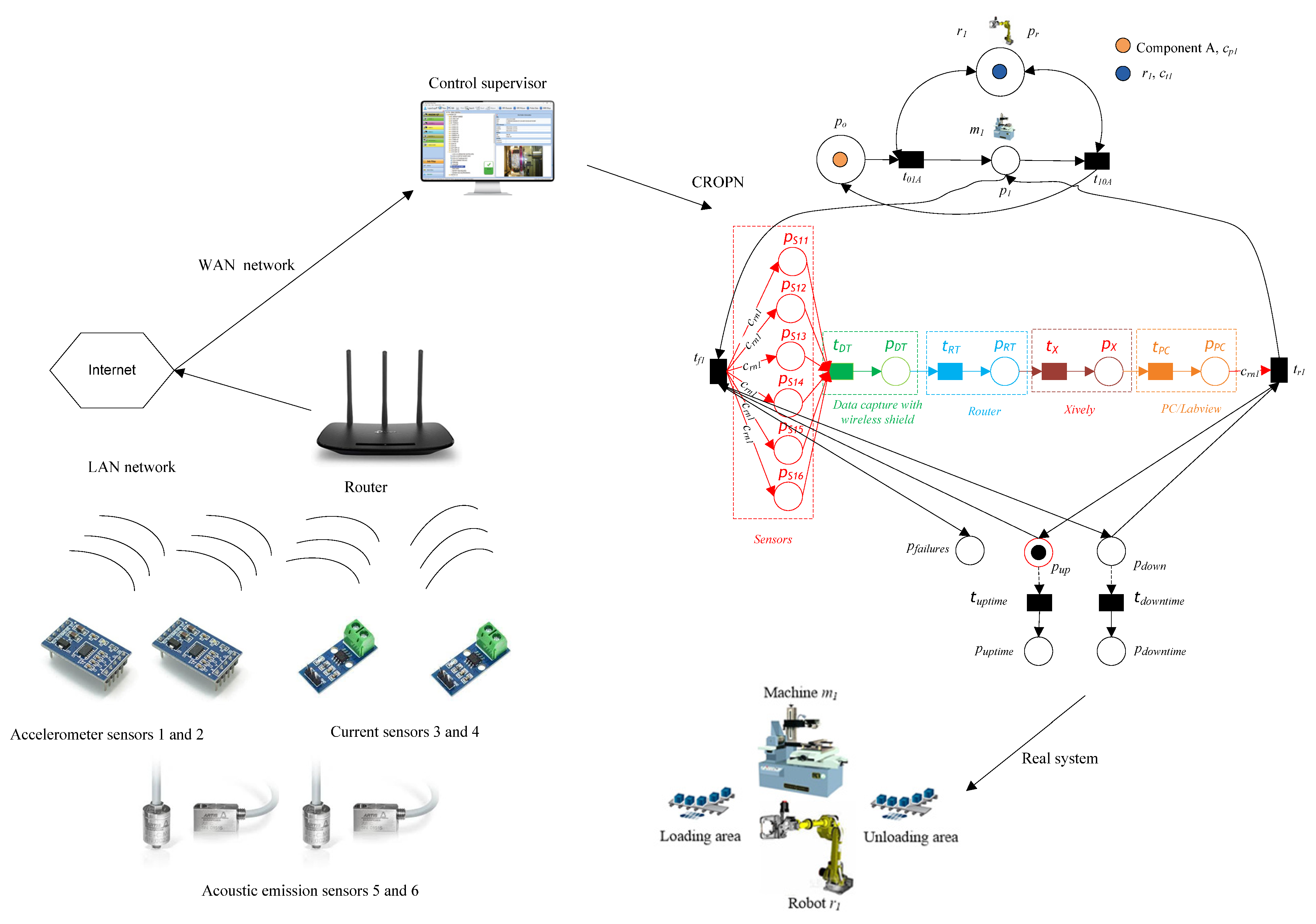
In AMSs, the “resource failure” represents a problem with temporal uncertainty. If a “resource failure” happens, we construct a “recovery subnet” that is capable of repairing it. The resource is then reusable. Moreover, for AMS to work effectively, reliably, and safely, “fault detection and treatment” should occur rapidly [21,22,23,30]. In this section, formal definitions are presented in order to build “recovery”, “detection”, and “treatment” networks for faults in AMS using IoT. Assume the system uses sensors to detect resource failures. The sensors transmit the data to the internet. Thus, the collected data can be viewed from any location in the world. Once the data have been sent to the internet, a computer will download them and use them to find and fix failures. Thus, if one of the resources fails, online operations can continue with the remaining resources. The value measured by the sensors is used as a “set point” or “threshold value” to help the system decide how to control itself. The flowchart and structure of the implemented systems are depicted in Figure 1.

The “open systems interconnection model” (OSI) application layer communication protocols, including “dynamic host configuration protocol” (DHCP) and “hypertext transfer protocol” (HTTP), were implemented for the capture and data processing system using C++ libraries. “Transmission Control Protocol” is implemented at the transport layer. The wireless connection between the sensors and the router is performed by employing the “Wi-Fi libraries” of the capture and data processing system to detect the “service set identifier” (SSID) and password for the “Wi-Fi protected access” or “wired equivalent privacy” security protocol, which is linked to the “Wi-Fi shield” [31]. Computer software is used to transfer all data to the cloud.

Let N be a CROPN with N = (P, T, C, I, O, K, M₀). Let N_IoT = ({p_i, p_Sij, p_DT, p_RT, p_X, p_PC}, {t_fi, t_ri, t_DT, t_RT, t_X, t_PC}, F_IoT, c_rni) be a “recovery net” of p_i based on IoT and M_IoTo represents initial states of the N_IoT, and F_IoT = {(p_i, t_fi), (t_fi, p_Sij), (p_Sij, t_DT), (t_DT, p_DT), (p_DT, t_RT),(t_RT, p_RT), (p_RT, t_X), (t_X, p_X), (p_X, t_PC), (t_PC, p_PC), (p_PC, t_ri)}, and M_IoTo(p_i) ≥ 0, where p_Sij, j > 0 is the sensor’s system for resource p_i failure sensing, p_DT represents the “data capture with wireless shield”, and p_RT denotes the router. The sensors p_Sj transmit the data to the Internet (represented by p_X), namely to the servers of Xively (“a platform designed for the IoT”). The collected data can be viewed from PC-LabVIEW (represented by p_PC). The transitions t_fi, t_ri, t_DT, t_RT, t_X, and t_PC indicate a "failure transition" of the resource p_i, a "recovery transition" of the resource p_i, a transition of the data capture, a transition of the router, a transition of the data capture, the transition of the Xively, and a transition of the PC/lab view, respectively. An unreliable net is constructed if CROPN (N, M_o) is combined with the recovery net (N_IoT, M_IoTo); this is represented by the expression (N_U, M_Uo) = (N_IoT, M_IoTo) ∥ (N, M_o), where ∥ represents the integration of (N_IoT, M_IoTo) and (N, M_o).

Based on the above notations, Algorithm 2 presents the IoT-based synthesis of CROPN. Algorithm 2 can immediately observe the change in sensors using the monitoring function software of the resource failure monitoring system. When a significant failure occurred in any machine in the system, the sensors’ amplitude also increased significantly. The software will provide a warning if the resource has a significant failure and the sensor data exceed the threshold. At this time, the machine tool number with the corresponding red symbol on the PC-LabVIEW represents an abnormal tool, while the green symbol denotes the tool is online and operating normally.

Algorithm 2Constructing CROPN based on IoT.

Input:The controlled CROPN with N = (P, T, C, I, O, K, M0); Output:The controlled CROPN based on IoT;   Insert places pDT, pRT, pX, pPC to the CROPN ;   Add transitions tDT, tRT, tX, tPC to the CROPN;   Draw arcs (tDT, pDT), (pDT, tRT), (tRT, pRT), (pRT, tX), (tX, pX), (pX, tPC), (tPC, pPC);   for (1 ≤ |PR| ≤ i++), do   Add a sensor transition tfi of the resource pi, pi ∈ PR;   Add a recovery transition tri of the resource pi, pi ∈ PR;   for (1≤ ψi ≤ j++), do/* ψi represents the number of sensors in pi*/   Add a sensor place psj for resource pi failure sensing;   Draw an arc from sensor transition tfi to a sensor psj;   Add an arc from sensor psj to a transition tDT;       end for   Draw an arc from the PC-LabVIEW pPC to a transition tri;   Add an arc from a transition tri to the resource pi; end for  Output: A controlled CROPN based on IoT;  End

3.2. Reliability Design of IoT-CROPN

The proposed unreliable net based on IoT was changed so that the reliability parameters of the AMS could be estimated. Note that both the “unreliable net” and the method for estimating reliability described in [22,32] were employed to determine the system’s reliability parameters. Let (N_U, M_Uo) be a CROPN based on IoT. Let N_RM = ({p_up, p_down, p_uptime, p_downtime, p_failures}, {t_fi, t_ri, t_uptime, t_downtime}, F_RM) be a “ reliability model” of CROPN based on IoT and M_RMo represent the initial states of the N_RM, and F_RM = {(p_up, t_fi), (t_fi, p_down), (p_down, t_ri), (t_ri, p_up), (p_up, t_uptime), (t_uptime, p_uptime), (p_down, t_downtime), (t_downtime, p_downtime)}, and M_RMo(p_up) =1, M_RMio(p_down) = 0, M_RMo(p_uptime) =0, and M_RMo(p_downtime) = 0, where p_up is the “on condition place”, p_down represents the “off condition place”, p_uptime denotes the on time counter place, p_downtime represents the downtime counter place, and p_failures denotes the number of occurred failures in a system. The transitions t_uptime and t_downtime represent an uptime deterministic transition and the downtime deterministic transition of the system, respectively. The reliability model of the CROPN based on IoT is constructed if a CROPN based on IoT (N_U, M_Uo) is combined with the reliability model (N_RM, M_RMo); this is represented by the expression (N_RU, M_RUo) = (N_RM, M_RMo) ∥ (N_U, M_Uo).

The “failure transition” t_fi and “recovery transition” t_ri of the CROPN based on IoT presented in Section 3.2 are connected to two places: the “off condition place” p_down and “on condition place” p_up {(p_up, t_fi), (t_fi, p_down), (p_down, t_ri), (t_ri, p_up)}, and the initial marking of the p_up = 1 and p_down = 0 that define the system’s down and up conditions. When a “failure transition” t_fi is fired, a token is removed from the “p_up” and a token is added to the “p_down”. The uptime and downtime of a system can be easily estimated by introducing a “time counter” expressed by a “test arc”, a downtime deterministic transition “t_downtime” and an uptime deterministic transition “t_uptime”, and two places a downtime place “p_downtime” and a uptime place “p_uptime” with arcs (p_up, t_uptime), (t_uptime, p_uptime), (p_down, t_downtime), (t_downtime, p_downtime), and the initial marking of the place p_uptime = 0 and the place p_downtime = 0. In addition, a place “p_failures” is inserted in the net to calculate the number of actual failures (denoted as “N_failures”). The parameters of reliability can be determined as follows:

“T_MTTF = T_uptime/N_failures.”

(11)

“T_MTTR = T_downtime/N_failures.”

(12)

“As = T_uptime/(T_uptime+ T_downtime).”

(13)

where T_MTTF, T_MTTR, and As represent the “mean time to failure”, the “mean time to repair”, and the “availability” of the IoT-based unreliable CROPN, respectively.

3.3. Computational Complexity

The computation time required to execute an algorithm can be considerable, depending mainly on the complexity of the algorithm. Computer scientists have devised a method for categorizing algorithms according to the number of operations they must execute; more operations require more time. Therefore, Theorems 1 and 2 demonstrate the computational complexity of Algorithms 1 and 2, respectively.

Theorem 1.

The computational complexity of Algorithm 1 is polynomial.

Proof. 

Algorithm 1 is used to show the deadlock avoidance policy for a CROPN model (N, Mo) (N, M_o) with N = (P, T, C, I, O, K, M_o). Algorithm 1 contains nested loops; let y represent the number of production process circuits (PPCs) in a CROPN model, i.e., y = |PPCs|. For each state M ∈ R(N, M_o), the liveness of each PPC will be verified using conditions 1–4; consequently, we refer to z as the CROPN reachable states, i.e., z = | R(N, M_o)|. The number of times “nested for loops” are conducted is yz when designing the deadlock avoidance policy for a CROPN model (N, M_o). Thus, the computational complexity of Algorithm 1 is O(yz). As the computational complexity of Algorithm 1 is polynomial, it is applicable to large-scale systems. □

Theorem 2.

The computational complexity of Algorithm 2 is polynomial.

Proof. 

Algorithm 2 is used to design the CROPN-model-based IoT (N_U, M_Uo) with (N_U, M_Uo) = (N_IoT, M_IoTo) || (N, M_o), where N = (P, T, C, I, O, K, M_o) and N_IoT = ({p_i, p_Sj, p_DT, p_RT, p_X, p_PC }, {t_fi, t_ri, t_DT, t_RT, t_X, t_PC}, F_IoT, c_rni, M_IoTo). Algorithm 2 has nested loops; let β be the number of machines (resources places) in a CROPN model, i.e., β = |P_R|, where PR is the set of resource places in (N_U, M_Uo). For each resource place p_i, where p_i ∈ P_R, the sensors will be connected to it using steps 7–11 of Algorithm 2; thus, we define the parameter λ to be the number of sensors in resource place p_i, and this is constant for all resource places in (N_U, M_Uo). When designing the CROPN-model-based IoT, the number of “nested for loops” executed is βλ. Therefore, Algorithm 2 has a computational complexity of O(βλ), is polynomial, and is appropriate for large-scale systems. □

3.4. Illustrative Example

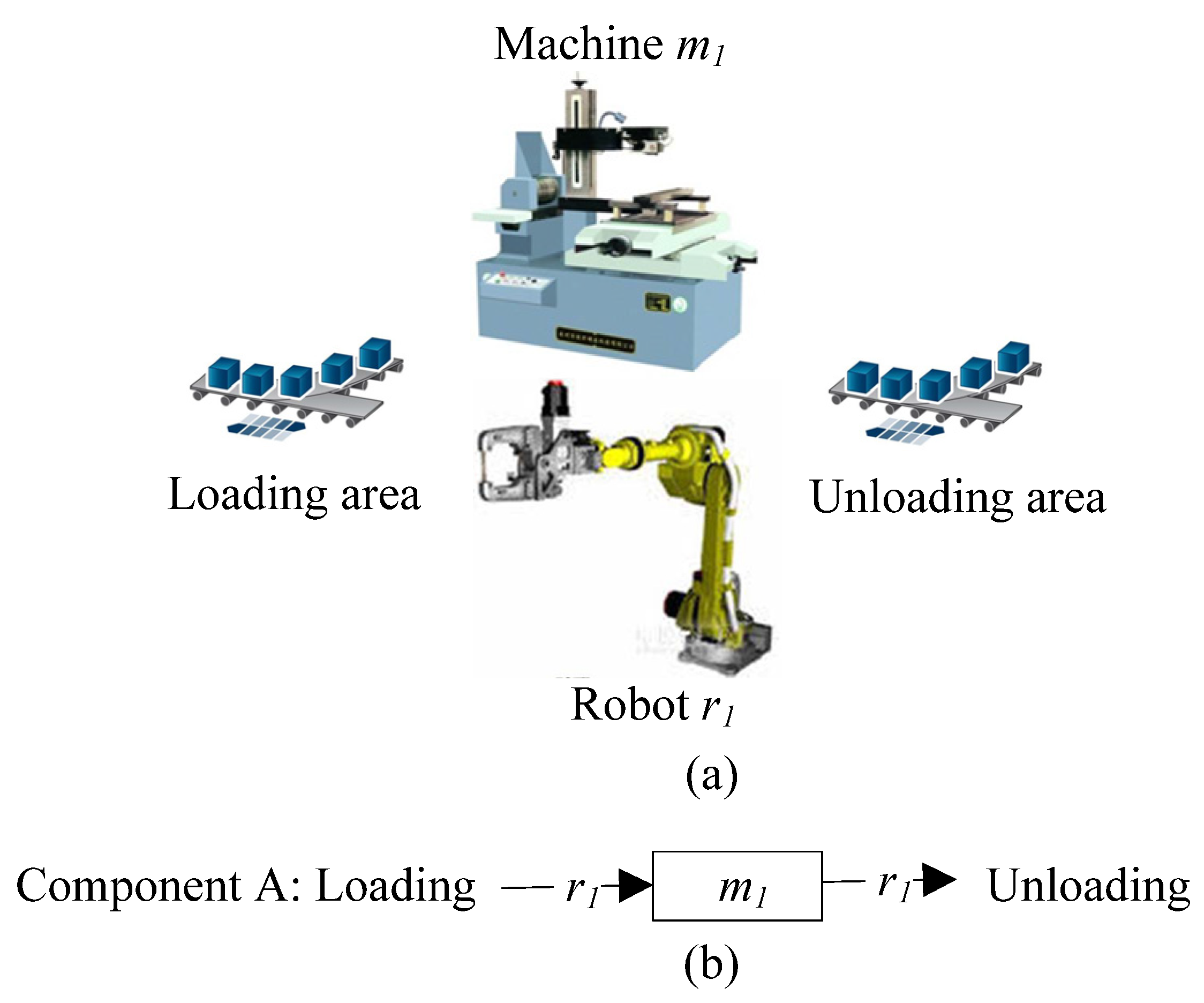
Consider the AMS [24] presented in Figure 2a to illustrate the CROPN construction. It consists of one CNC machine m₁ (operation resource), one robot r₁ (material handling equipment resource), and a load/unload station. The AMS produces one component type A. The AMS operation route is presented in Figure 2b.

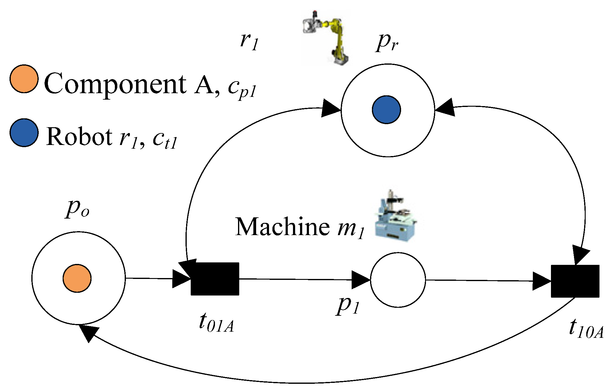
The developed CROPN is shown in Figure 3. As illustrated in Figure 3, places p₁ and p_r model machine m₁ and robot r₁, respectively. Transitions t_01A and t_10A model the transporting component A to/from p₁, respectively. The initial marking of the developed CROPN model is M_o(p_o, p₁ p_r) = M_o(c_p1, 0, c_t1), where c_p1 indicates that a raw component A is available at the load/unload station p_o, c_t1 denotes robot r₁, which means that the robot r₁ is idle and can transport the raw component A, and M_o(p₁) = 0 means that the machine m₁ is free and available to process a raw component A. The component process route is as follows: a component A is placed at the place p_o, the robot r₁ transports a component to the machine m₁ (p₁) via a transition t_01A, and if the processing time of the machine m₁ is finished, the robot r₁ transports the completed component via a transition t_10A to the place p₀. The CROPN’s behavior is as follows: When a transition t_01A is enabled, it fires, and selects, respectively, from places p_o and p_r, one token c_p1 and one token c_t1. If a transition t_01A is fired, it adds, respectively, to places p₁ and p_r, one token c_p1 and one token c_t1. When the machine’s m₁ processing time is finished, a transition t_10A is enabled, and it selects, respectively, from places p₁ and p_r, one token c_p1 and one token c_t1. If a transition t_10A is fired, it adds, respectively, a token c_p1 and a token c_t1 to the p_o and the p_r. According to Algorithm 1, the CROPN has no production process circuits that meet condition 6. Thus, it is live.

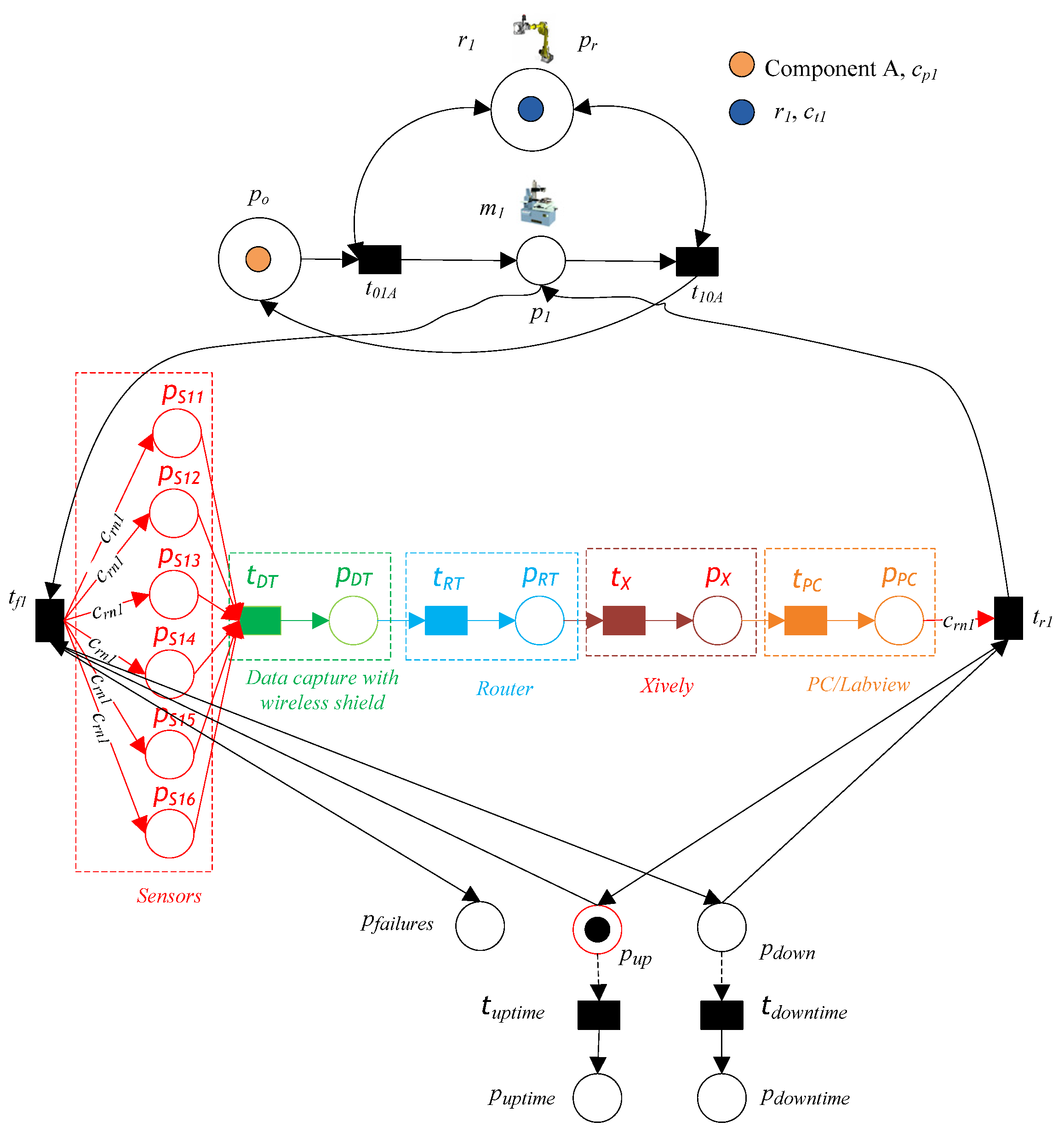
Figure 4 illustrates the CROPN based on an IoT network for the system depicted in Figure 3 in order to demonstrate how to recognize and treat tool wear. We used a part of a mill dataset to evaluate the tool status under a single operational condition, as performed by [33]. This data set was collected through controlled laboratory experiments of milling machine operations performed using a variety of parameters, including depth of cut, feed rate, and material type. The collection of data was sampled by three different types of sensors (“acoustic emission sensor”, “vibration sensor”, and “current sensor”) at various positions [33].

In [33], a high-speed data acquisition board with a maximum sampling rate of 100 kHz was used to transmit the data. The output of the sampled data was utilized by the signal processing software. Multiple sensor signals were preprocessed. In most instances, the signal was amplified to meet equipment threshold requirements. Specifically, the data from the “acoustic emission sensors” and the “vibration sensors” were amplified to be within the range of ±5 V for maximum load, taking into account the equipment’s maximum permitted range. The signals were screened using a “high-pass filter”, and the “vibration sensor” signals were further screened using a “low-pass filter”. The corner frequencies were selected based on the noise noticed on an “oscilloscope”. On the oscilloscope, 180 Hz of periodic noise was observed for the vibration signal, matching the third harmonic of the primary power source. Consequently, 400 Hz was chosen as the corner frequency for the “low-pass filter”. The 1 kHz “high-pass filter” was selected. The range of the “acoustic emission sensor” ends at 8 kHz. Thus, observations exceeding this frequency cannot be attributable to any machining process occurrence. Because it unnecessarily muddies the signal, it was filtered out.

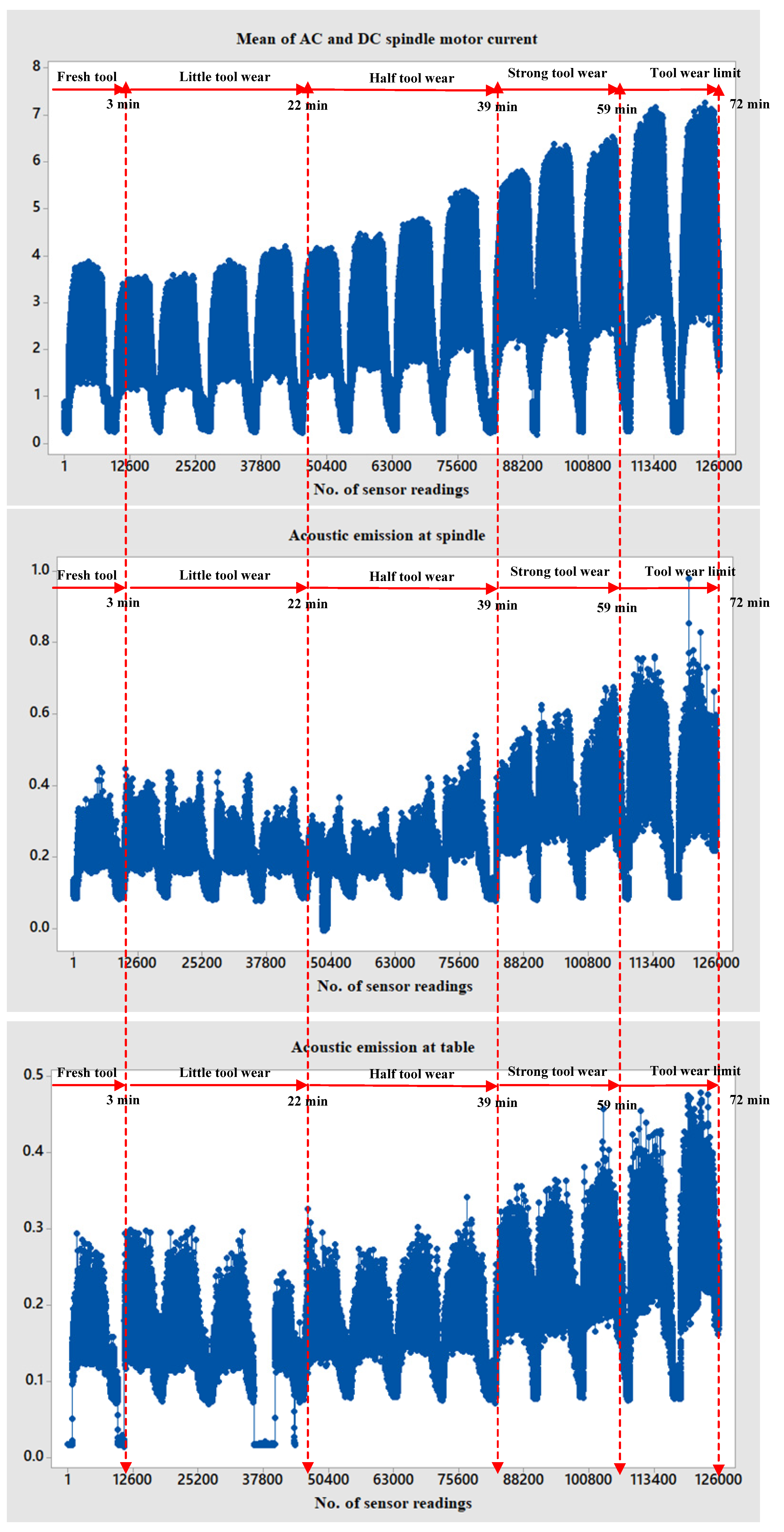
As seen in Figure 4, the system uses six sensors for tool failure sensing: the current sensors p_s1 and p_s2, which, respectively, gauge variations in an alternating current (AC) and a direct current (DC) spindle motor; the accelerometer sensors p_s3 and p_s4, which, respectively, gauge table and spindle vibrations; and the acoustic emission sensors p_s5 and p_s6, which, respectively, measure acoustic stress wave effects at the table and spindle for the diagnosis of a tool break. There are multiple phases to the process of transmitting data to the Internet. The sensors p_s1, p_s2, p_s3, p_s4, p_s5, and p_s6 first take the readings and send them to the “Wi-Fi wireless shield” (represented by t_DT and p_DT). The shield then transfers the data to a “wireless router” (denoted by t_RT and p_RT). Integrating objects into a communication network is an important component of the IoT. In other words, it symbolizes a new method in which all objects are integrated into the Internet and interact in real time. Practically, it is built on the integration of sensors, equipment, and “household” items with the internet via “wired or wireless networks”. The use of this method is achievable, and its implementation will be cost-effective due to the Internet’s global reach. It will enable the “sensors” to be connected in “homes”, “workplaces”, and various “automation operations”. Thus, every object can be linked to a web environment in order to save all of its data and display it in the actual world. The objective of this research is to introduce the PC-LabVIEW-based system designed to communicate Internet data to the CROPN. Using a PC equipped with Labview (represnted by t_PC and p_PC), the cloud-stored data is downloaded for processing and transmission to the CROPN. Through the OPC communication standard, the CROPN is responsible for executing the PC-LabVIEW-programmed fault detection and treatment control (communication between the CROPN and PC-LabVIEW). Figure 5 shows the reliability design of the net illustrated in Figure 4.

The system depicted in Figure 6 is the “graphical user interface” (GUI) that enables communication with the sensor system and presents the collected information. Consequently, it supervises and monitors the operation. If the sensor data exceed the threshold, the CROPN executes the system’s action.

The information gathered by the “sensors” and sent to the Internet is depicted in Figure 7. It enables the filtering and graphing of data to identify potential patterns or important events. Regardless of the exact location of the sensors, the data can be accessed from anywhere on Earth.

4. Experimental Results

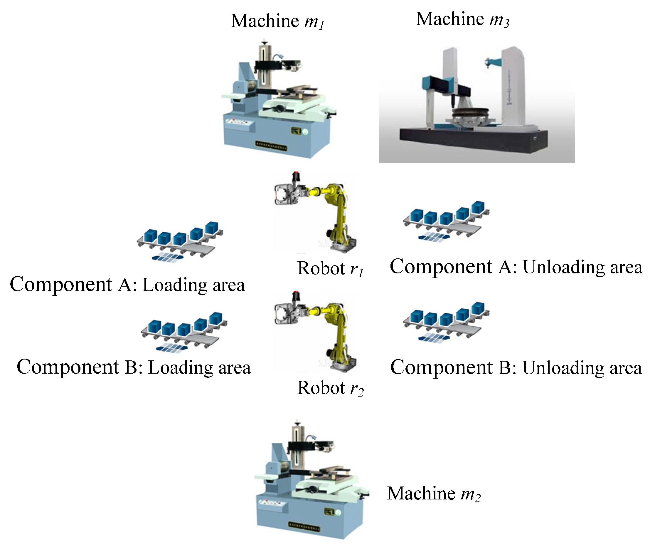
This section uses an existing automated manufacturing system in [21,24] to describe the implemented sensor system. The system is illustrated in Figure 8. It includes three machines, m₁–m₃ (resources for operations); two robots, r₁ and r₂ (resources for material handling equipment); and a load/unload station. The AMS produces two component types, A and B. The experimental conditions and parameters were determined by industry applicability and manufacturer-recommended settings. The conditions and parameters of the system were as follows: For machine 1, the cutting speed was set to 200 m/min, which corresponds to 826 rev/min, the depth of cut was 1.5 mm, and the feed rate was 0.5 mm/rev, which translates to 413 mm/min. For machine 2, the cutting speed was set to 200 m/min, the depth of cut was 0.75 mm, and the feed rate was 0.25 mm/rev, which translates to 206.5 mm/min. Cast iron (component A) and stainless steel J45 (component B) were used as the materials. The collection of data was sampled by three different types of sensors (“acoustic emission sensor”, “vibration sensor”, and “current sensor”) at various positions.

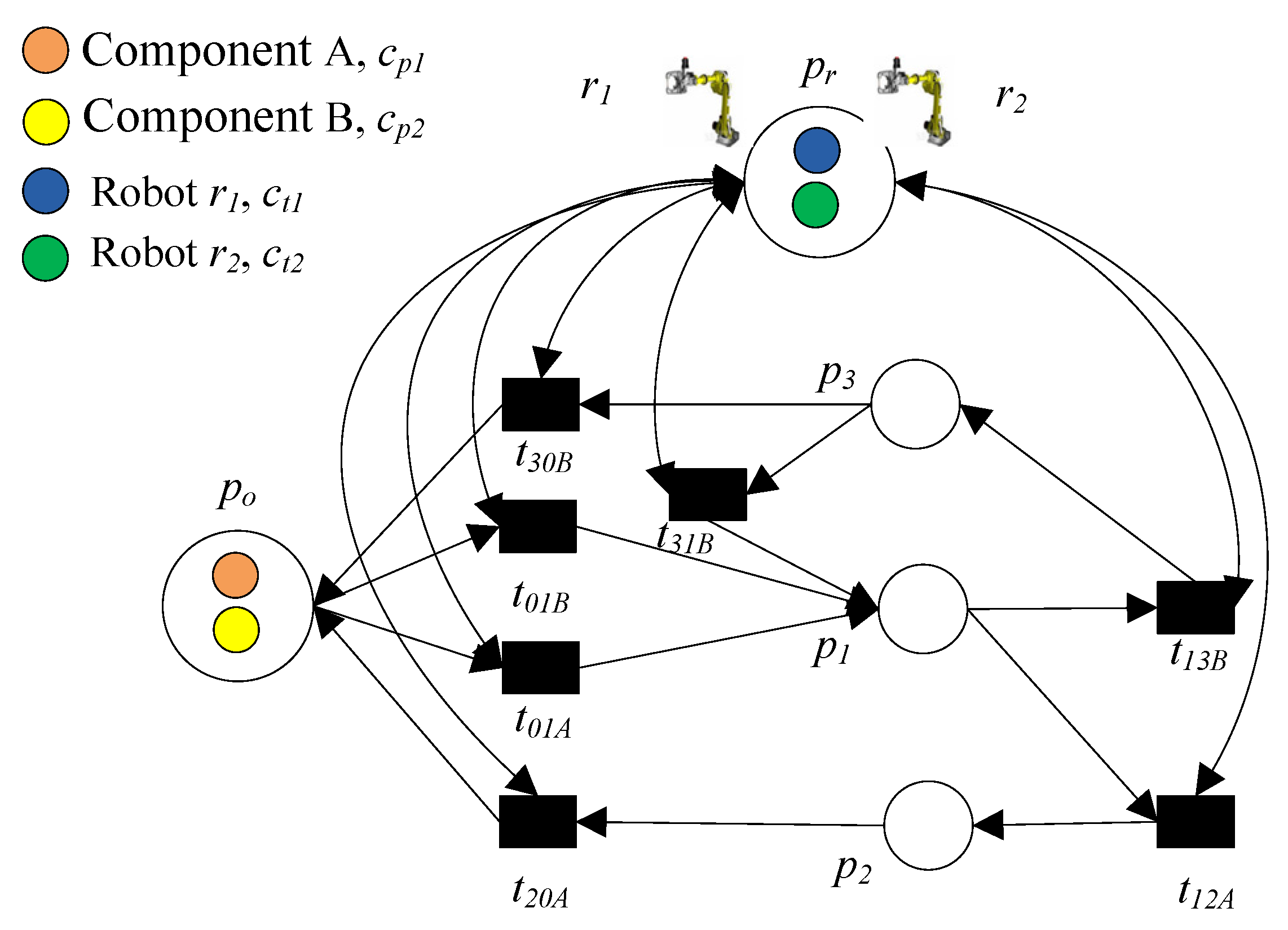
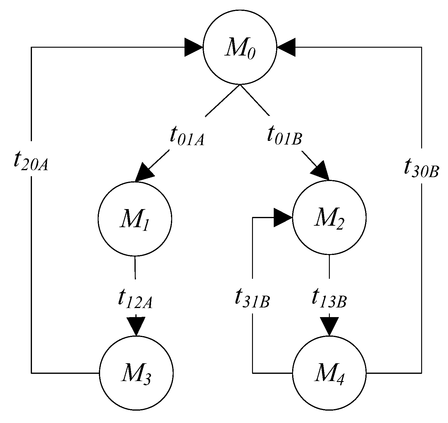
The description of places, transitions, and colors in the CROPN model presented in Figure 9 is as follows: Places p₁, p₂, p_r, and p₀ represent a machine m₁, a machine m₂, a transportation place for robots r₁ and r₂, and the loading and unloading station, respectively. Transitions t_01A, t_12A, t_20A, t_01B, t_13B, t_31B, and t_30B model, a transporting of the component A from the p₀ to the machine m₁ by robots r₁, a transporting of the component A from the machine m₁ to the machine m₂ by robots r₁, a transporting of the component A from the machine m₂ to the p₀ by robots r₁, a transporting of the component B from the p₀ to the machine m₁ by robots r₂, a transporting of the component B from the machine m₁ to the machine m₃ by robots r₂, a transporting of the component B from the machine m₃ to the machine m₁ by robots r₂, and a transporting of the component B from the machine m₃ to the p₀ by robots r₂, respectively. The colored tokens c_p1, c_p2, c_t1, and c_t2 represent component A, a component B, a robot r₁, and a robot r₂, respectively.

The initial states of the developed CROPN are M_o(p_o, p₁, p₂, p₃, p_r) = M_o({c_p1, c_p2}, 0, 0, 0, {c_t1, c_t2}), where c_p1 and c_p2 indicate, respectively, that raw components A and B are available at load/unload station p_o; c_t1 and c_t2 denote, respectively, robots r₁ and r₁, which mean that the robot r₁ is idle and can transport the raw component A and the robot r₂ is idle and can transport the raw component B; and M_o(p₁) = M_o(p₂) = M_o(p₃) = 0, which mean that the machines m₁–m₃ are free and available to process raw components. In addition, the following describes the process routes of the components A and B:

(1)

Component A is available in the place p_o and the robot r₁ transports it to the place p₁ (m₁) via a transition t_01A. If the processing time of the m₁ is finished, the r₁ transports the component from m₁ to the place p₂ (m₂) via a transition t_12A. If the processing time of the m₂ is finished, the robot r₁ transports the completed component via a transition t_20A to the place p₀.

(2)

Component B is available in the place p_o and the robot r₂ transports it to the place p₁ (m₁) via a transition t_01B. If the processing time of the m₁ is finished, the r₂ transports the component from to the place p₃ (m₃) via a transition t_13B, when the component has no defects, the r₂ places the completed component via a transition t_30B to the place p₀; otherwise the component returns to the place p₁ (m₁) via a transition t_31B, then to a transition t_13B, a place p₃, a transition t_30B, and a place p₀.

To determine if the developed CROPN is live, reconsider the net presented in Figure 9. Figure 10 depicts its reachability markings and can be stated as

M₀ = ({c_p1, c_p2}, 0, 0, 0, {c_t1, c_t2}).

M₁ = (c_p2, c_p1, 0, 0, {c_t1, c_t2}).

M₂ = (c_p1, c_p2, 0, 0, {c_t1, c_t2}).

M₃ = (c_p2, 0, c_p1, 0, {c_t1, c_t2}).

M₄ = (c_p1, 0, 0, c_p2, {c_t1, c_t2}).

The CROPN consists of a PPC: e₁ = {p₁, t_13B, p₃, t_31B}. We assume that p₁, p₂, and p₃ each have a capacity of one. The control condition 6 stated in Equation (8) is employed to determine the number of available spaces in an e₁, which are displayed in

Table 1. The free spaces in an e₁.

State	K(e1) = ΣK(pi, e1)	M(e1) = ΣMk(pi, e1)	S′(e1) = K(e1) − M(e1)
0	2	0	2 ≥ 1
1	2	1	1 ≥ 1
2	2	1	1 ≥ 1
3	2	0	2 ≥ 1
4	2	1	1 ≥ 1

. As illustrated in Table 1, the condition 6 was achieved for all markings displayed in Figure 10, and the subnet e₁ was live. Thus, we can concluded that the developed CROPN was live.

Next, Figure 11 illustrates the IoT-based CROPN and reliability model for the system depicted in Figure 9 in order to demonstrate how to recognize and treat faults. As seen in Figure 11, we have the following nomenclature: Places p_s11 and p_s21 represent the “current sensors”, which gauge changes in an AC of the spindle motor for machines m₁ and m₂, respectively; p_s12 and p_s22 model the “current sensors”, which gauge changes in a DC of the spindle motor for machines m₁ and m₂, respectively; p_s13 and p_s23 represent accelerometer sensors that gauge table vibration for machines m₁ and m₂, respectively; p_s14 and p_s24 model the “accelerometer sensors” that gauge spindle vibration for machines m₁ and m₂, respectively; p_s15 and p_s25 represent the “acoustic emission sensors” that gauge “acoustic stress wave” impacts at the table for machines m₁ and m₂, respectively; p_s16 and p_s26 model the “acoustic emission sensors” that gauge “acoustic stress wave” impacts at the spindle for machines m₁ and m₂, respectively. In addition, places p_DT, p_RT, p_X, p_PC, p_up, p_down, p_uptime, p_downtime, and p_failures represent the “data capture with wireless shield,” the router, the transmitting the data from sensors p_Sij to the Internet, the PC-LabVIEW, the “on condition place” for machines m₁ and m₂, the “on condition place” for machines m₁ and m₂, the “off condition place” for machines m₁ and m₂, the “uptime place” for machines m₁ and m₂, the “downtime place” for machines m₁ and m₂, and number of actual failures in machines m₁ and m₂, respectively. Finally, transitions t_f1, t_f2, t_r1, t_r2, t_DT, t_RT, t_X, t_PC, t_downtime, and t_uptime represent the failure of the machine m₁, the failure of the machine m₂, the recovery of the machine m₁, the recovery of the machine m₂, the data capture, the router, the Xively, the PC-LabVIEW, the downtime deterministic for machines m₁ and m₂, and the uptime deterministic for machines m₁ and m₂, respectively.

5. Performance Evaluation

Finally, a MATLAB-based GPenSIM tool [20,24,30,34,35] was used to execute verification and validation of the constructed IoT-based CROPN and the reliability model presented in Figure 11. The GPenSIM tool was developed in order to simulate and evaluate AMS. Using MATLAB R2015a, the developed code for the reliability model was executed. The length of the simulation (denoted as T_Simulation) was 450 min.

Table 2. Data of the machine maintenance for the model illustrated in Figure 11.

Machine	Processing Time (min)		TMTTF (min)		TMTTR (min)
	Com. A	Com. B	Without Sensor System	With Sensor System	tt1	tt2
m1	5	7	74	Based on sensor system	10	-
m2	6		84		-	13
m3	-	2	-		-	-

provides data on machine maintenance for the system depicted in Figure 10. Moreover,

Table 3. Comparison of the proposed IoT-CROPN shown in Figure 11 with existing methods.

	Performance
	Throughput (Components)		Throughput Time (min/Component)		Utilization (%)
	Com. A	Com. B	Com. A	Com. B	m1	m2	m3
Al-Shayea et al. [30]	26	27	17.31	16.67	76.23	34.98	13.45
Kaid et al. [22]	28	29	16.07	15.52	81.61	37.67	14.35
Al-Ahmari et al. [23]	27	28	16.67	16.07	80.94	36.77	13.90
Alzalab et al. [36]	29	29	15.52	15.52	83.56	38.06	14.19
IoT-CROPN	29	30	15.52	15	84.68	39.19	14.86

summarizes the result of the simulation, which contains the total components that go through the time of simulation (denoted as N_Throughput), the throughput time for component (represented by T_Throughput), which can be expressed as

$$T_{Throughput}=\frac{T_{Simulation}}{N_{Throughput}},$$

(14)

and the utilization of the machine, that can be formulated as

$$U_{Machine}=\left(\frac{T_{Machine}}{T_{Simulation}}\right)·100$$

(15)

where U_Machine and T_Machine represent the utilization of the machine and the total occupation time of the machine, respectively.

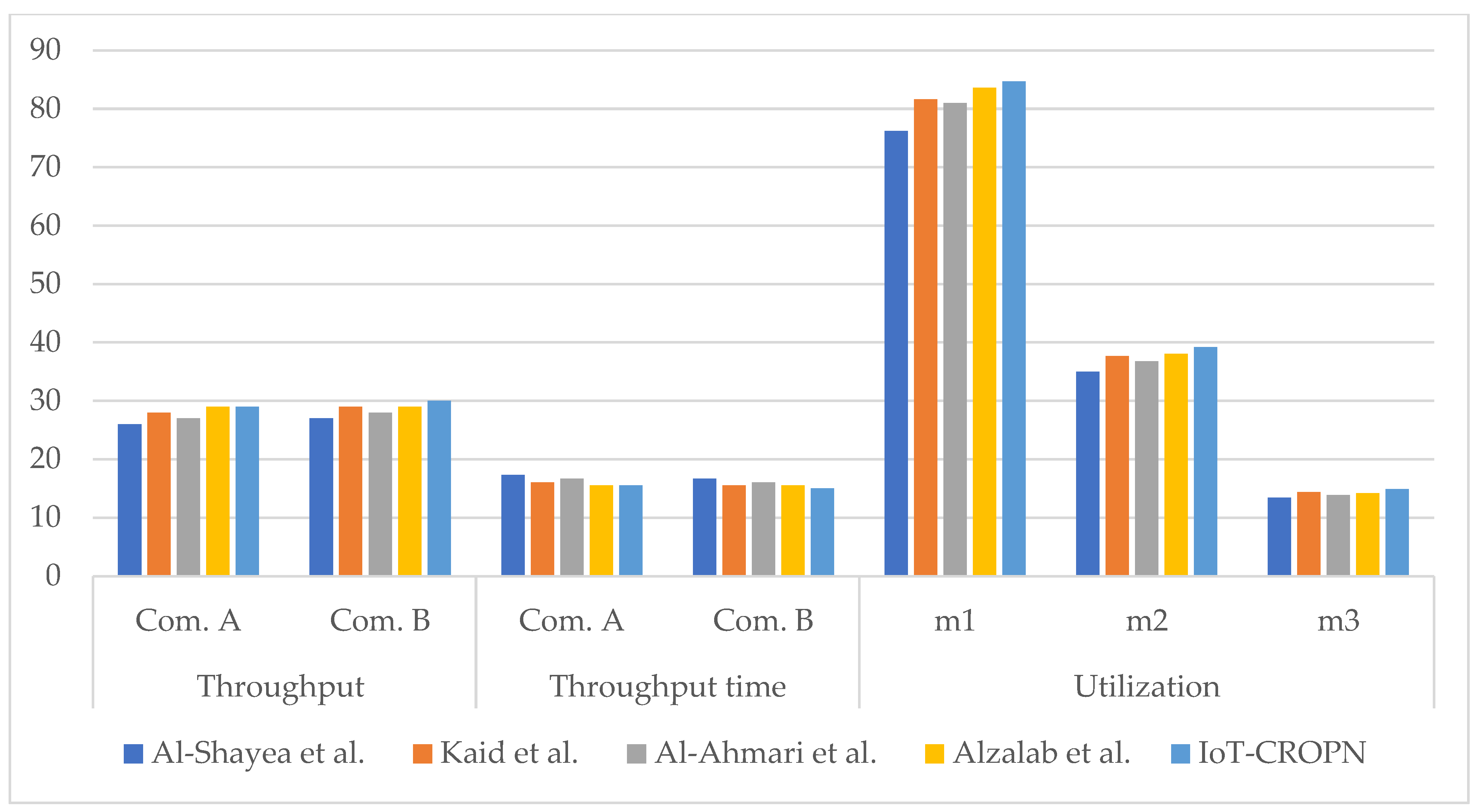
As depicted in Figure 12, the results of these experiments were compared with [22,23,30,36], where the same conditions and parameters were used for all studies. In terms of “throughput”, “throughput time”, and “utilization”, the results show that the IoT-based CROPN outperformed the other approaches. Moreover,

Table 4. The parameters of the reliability for the IoT-CROPN shown in Figure 11.

	Reliability Parameter
	Tuptime (min)	Tdowntime (min)	As (%)
Al-Shayea et al. [30]	347	103	77.11
Kaid et al. [22]	372	78	82.67
Al-Ahmari et al. [23]	384	66	85.53
Alzalab et al. [36]	394	56	87.55
IoT-CROPN	397	53	88.22

contains the reliability metrics of the IoT-based CROPN: “uptime”, “downtime”, and “availability”. The availability of the model was observed to be 88.22%, outperforming two existing approaches.

6. Conclusions

In this paper, we emphasize the significance of techniques, tools, and procedures designed to support automatic threat (i.e., fault, error, and failure) diagnosis and recovery due to the immense interest and development of IoT-based cyber-physical systems in AMS, where a certain degree of adaptability is crucial. We propose an IoT-based CROPN to facilitate self-detection and self-treatment of failures and to obtain essential reliability measurements in the IoT-based CROPN, such as “uptime”, “downtime”, and “availability”. Existing system examples are used to demonstrate the effectiveness of the developed technique. First, the tool wear condition of a CNC milling machine was evaluated using an IoT-based CROPN that provided a systematic classification of tool wear status. This technique can lead to more effective monitoring of tool replacement due to a more effective evaluation of tool wear. First, “sufficient and necessary conditions” were presented for the liveness of the CROPN. Second, we developed a “fault diagnosis and treatment” method, which combines the obtained CROPN with IoT to guarantee the reliability of the CROPN. A simulation tool was used to verify, validate, and analyze the reliability of the IoT-based CROPN, and the results were compared with those reported in the literature.

The advantages of the IoT-based CROPN are as follows:

(1)

Compared to the research in [22,23,30,36], it has been demonstrated to be simpler in configuration and more effective at overcoming the deadlock problem, “fault diagnosis and treatment”, and designing CROPN reliability.

(2)

It provides a hybrid model that is simultaneously simulated in real time and on the plant floor.

(3)

It was experimentally validated to demonstrate how to evaluate performance and monitor tool status on various machines.

Future research will address other discrete variables, such as product quality, overall energy utilization, reconfiguration of an AMS, and product rescheduling. In addition, operations on an “intelligent vehicle highway system” (IVHS) are highly non-linear and subject to rapid environmental change. In order to guarantee safe travel for humans, accurate diagnosis and reliable sensor data are required. Therefore, an internet-of-things-based CROPN can be employed to improve IVHS capacity and safety on the highway. Finally, in some occurrences of multiple failures, symptoms may be mutually exclusive. In large-scale problems, it may not be as simple to recognize and model these occurrences that deviate from the default model. Thus, a technique for capturing these occurrences should be designed.