Online System Prognostics with Ensemble Models and Evolving Clustering

Abstract

An online evolving clustering (OEC) method equivalent to ensemble modeling is proposed to tackle prognostics problems of learning and the prediction of remaining useful life (RUL). During the learning phase, OEC extracts predominant operating modes as multiple evolving clusters (EC). Each EC is associated with its own Weibull distribution-inspired degradation (survivability) model that will receive incremental online modifications as degradation signals become available. Example case studies from machining (drilling) and automotive brake-pad wear prognostics are used to validate the effectiveness of the proposed method.

1. Introduction

Prognostics for a system or a process focuses on predicting the remaining useful life (RUL), and the presence of incipient failures within a foreseeable horizon. It is a critical function of prognostics and health management (PHM) systems that utilize results from diagnostics and prognostics modules to monitor the severity of faults and the overall trajectory for a system’s state of health. This type of knowledge, acquired or predicted, facilitates management decisions and actions related to maintenance, logistics, and personnel [1,2]. In the literature, diagnostics and prognostics are typically combined within a condition-based monitoring (CBM) module where various model-based, data-driven, and hybrid methods have been proposed. The choice and implementation of a CBM program are dependent on the nature of the system, associated critical components, how each problem is framed, and the depth and coverage of expert knowledge to be incorporated into solving them [3].

Cluster analysis or clustering focuses on identifying major groups in data such that data in the same group has more similarity than data from a different group [4,5]. As a result, it partitions a single set of data into several subsets so the system can zoom into each subset as a sub-problem. It is a commonly used method in CBM applications as a pre-processing step to reduce complexity and noise in the data to “divide, conquer and simplify” otherwise very complex problems. Clustering is an unsupervised task because there are no truth values or labels. To this end, clustering is distinctly different from other popular methods in CBM, such as “classification”, where the truth or label information is assumed to be available. Clustering methods, such as fuzzy c-means (FCM) [6], k-means clustering [7], and mountain clustering [8], are a few of the most popular algorithms, and they have been widely applied for exploratory data mining and visualization, object detection, novelty detection, and knowledge discovery in a wide range of applications. Among these methods, DBSCAN [9] received a lot of attention recently due to its performance, flexibility, and the ability to represent large amounts of data where the clusters may not necessarily be represented by exactly the same set of features, and the number of clusters may not have to be specified. Online evolving clustering (OEC), a relatively new class of clustering methods, enables the adaptation in both their structure and parameters [10,11,12,13,14]. Due to the added capability of performing incremental modifications to the model, it is well suited for data with indefinite length (or data streams). In [15] it was reported that its performance is on par with a physics-based model for complex systems.

With the advances in machine learning, and the access to large-scale datasets shared across the academia and industry sectors, there has been an acceleration in the development of new techniques. In [16], challenges in data alignment and noise reduction mechanisms were addressed with ARMA graph convolution, adversarial adaptation, and multi-layer multi-kernel local maximum mean discrepancy (ML-LMMD). To address the increasingly common issues associated with multi-sensors and uncertainty quantification in the predicted RUL information, Ref. [17] proposed a gated graph convolutional network (GCCN) which simultaneously models the temporal and spatial dependencies in the data. A graphical neural network combines the capability and learning mechanisms of modern neural networks for diagnostics and prognostics progressions and maintains learned knowledge/state representations [18]. Probabilistic approaches, such as Bayesian networks with recurrent mechanisms, have been improved for generic RUL problems, where uncertainties from different sources are handled by separate layers in the network [19]. Attention mechanisms were designed and implemented for semi-supervised fault detection by exploiting dependencies between similar data and neighboring nodes in the network in an effort to deal with imperfect information that arise due to natural signal variation under different working conditions and controls for different planned tasks [20]. In [21], a hybrid robust convolutional autoencoder (HRCAE) and a parallel convolutional distribution fitting (PCDF) module was constructed to conduct unsupervised anomaly detection of machine tools under a noisy environment when labels of data may not be available most of the time. To deal with frame-based inputs where repetitions and variable length of data and similar inputs have been addressed with dynamic time warping and PCA [22]. In [23] two novel neural network variants were proposed, namely the growing neural network (GNN) and a variable sequence LSTM for the diagnosis, prognosis, and health monitoring framework. The domain application was on an aerospace industry where the accuracy of predicted results have implications to ensure safe and successful completion of planned flight tasks, and the models improved management of repair and maintenance costs.

In the work of [23], the common practice of transfer learning in certain ML domains (i.e., natural language processing) have been surveyed with limited references to CBM applications. The authors break down the tasks into three methods, as follows: model and parameter transfer, feature matching, and adversarial adaptation with examples on machinery diagnostics and prognostics. For the consistently increasing complexity of modern-day industrial systems, Ref. [24] emphasized the need for a comprehensive integrated health monitoring (IHM) system using the vehicle as an example of the type of systems of systems that are rapidly growing in complexity. Traditionally, the OEM’s focus is mainly on the improvement of diagnostics capabilities with key sub-systems, but the trend is now heading toward a more integrated approach and accurate prognostics information. This is due to the demand from the customers, as well as from the OEMs, due to the significance of these tools for discovering the emerging quality issues and quantifying the associated warranty costs. Hybrid approaches that incorporate multiple RUL learning and prediction mechanisms continue to be investigated to improve the final model’s capability to generalize information to balance between robustness and accuracy for extremely challenging problems, such as RUL estimation of modern lithium-ion batteries [25].

For human behaviors and early detection of medical conditions, steady progress was made with relatively recent ML architectures. Deep structured models, such as EEGNet and DeepconNet, were investigated and were shown to yield high precision results for autism spectrum disorder (ASD) with EEG signals in a transfer learning setting [26]. Researchers have also investigated, from the healthcare system and practitioner’s perspective, the implications of AIML-aided diagnosis and prognosis in practice, as well as their educational impacts on the society [27]. Furthermore, as large-scale data collection becomes more prevalent, the sheer volume of data poses significant challenges in all phases of machine learning-based systems and data-driven operations. In [28] the latest advances in few-shot learning (FSL) are studied to facilitate learning from a few samples with prior knowledge. In [29], the team focused on similar issues with applying online learning methodologies, where feature extraction and subsequent model learning were performed online, meaning it goes through a few data points (flow through the data stream) at a time to greatly reduce the computational footprint.

In this paper, the focus is on the prognostics applications of a mutual information-based Gustafson–Kessel-like clustering algorithm (MIRGKL) embedded with local approximation functions. This work is inspired by an online evolving clustering (OEC) algorithm originated from an extended version of the Gustafson–Kessel (GK) clustering algorithm [10]. The MIRGKL applies the mutual information formulation to the Mahalanobis distance to produce a conservative assessment of the similarity calculations between objects. With the filtered version of the similarity measure, choices are made between cluster maintenance actions, including the creation of a new cluster, merging of existing clusters, or update of an existing cluster. Degradation information of a system is typically made available much less frequently but is necessary to train cluster-specific degradation (survival) models according to a cluster assignment. In the case when the cluster assignment and degradation information are asynchronous, inferred degradation information needs to be estimated, such that the learning of cluster-specific degradation function takes place subsequently right after cluster assignment. The modifiable cluster-specific degradation model is based on the linearized version of the well-known Weibull survival function that can be learned in real-time. Note that while we do not put emphasis on insignificant clusters (i.e., small population and/or low utilization), the frequencies of their occurrences are related to novel emerging patterns and, therefore, may be of interest for diagnostics purposes for mission critical systems [30,31]. Treating prognostics as a function learning and prediction problem makes it well suited for various methods that are designed for this purpose. Bundling with an evolving clustering method allows such a learning-based system to start from scratch, initiate RUL predictions early due to the lower data requirement, and to leverage modern incremental training to keep track of newly available data with a small footprint on the computational requirement. Other state of the art tools for tackling similar problems (RUL estimation) as a function approximation problem include support vector regression [32], Kalman filter [33], and deep neural networks [34]. In addition, decision trees and tree-based methodologies, due to their flexibility to incorporate a mixture of related variables, ease of interpretation for predictive purposes, and robustness in performance, continue to be one of the most applied method for many real-world applications [35,36].

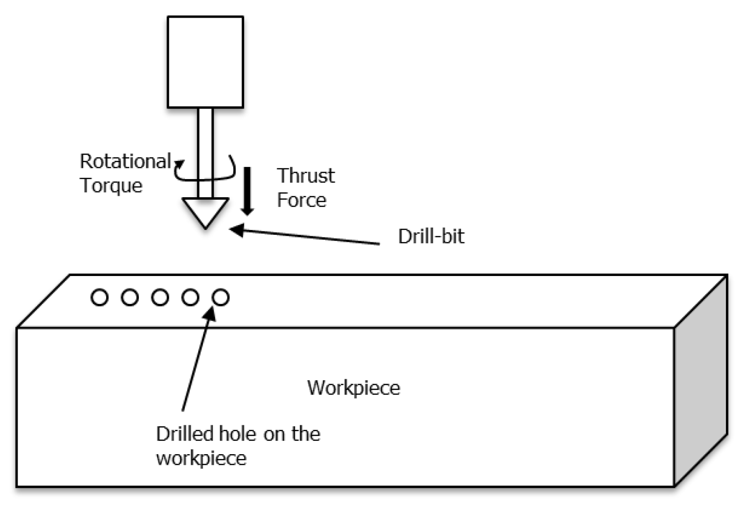
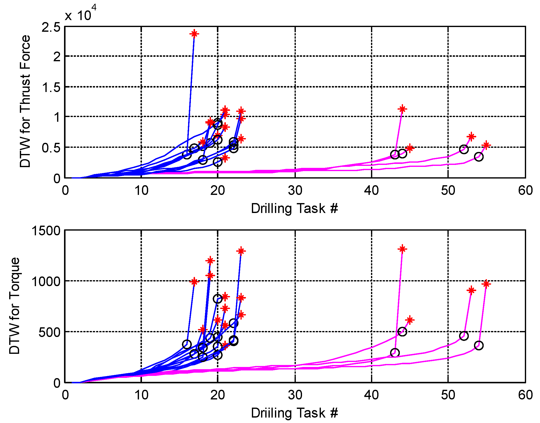
As in most diagnostics and prognostics problems, the signal processing and feature extraction procedure comes from the physical understanding of the problem. To demonstrate the effect of the proposed generic prognostics method, we kept feature extraction at very high levels. For the drill-bit example, we mainly rely on the dynamic time warping (DTW) algorithm to process signal profiles (as a while) acquired during the drilling process with varying lengths. For brake wear monitoring, a more generic descriptive statistics in the form of pre-defined fixed interval distributions is used to summarize the drive content as the primary features. After signal processing and feature processing, MIRGKL with local functions are applied for prognostics purpose.

Therefore, the goal of the research is to develop a generic data-driven algorithm that automatically learns to perform prognostics tasks through the dynamic construction of multiple local (cluster-specific) degradation models and to apply the appropriate model to predict the remaining RUL of a machine or subcomponent. With the advancement in sensing and computer hardware (cloud), we aim at using this research for further development of common and generic learning and computer modules as the essential part of a larger CBM ecosystem.

The rest of the paper is organized as follows. Section 2 formally introduces the MIRGKL clustering algorithm with the proposed addition of cluster-specific degradation functions. Section 3 demonstrates the application of the proposed prognostics algorithm on two real-world examples, namely (i) a drill-bit life prediction, and (ii) brake pad wear prediction. Finally, Section 4 summarizes the results and discusses directions for future research.

2. Method: Clustering with Embedded Local Functions

This section formally introduces the proposed OEC-based prognostics method. To this end, we first describe the mutual information-based recursive Gustafson–Kessel-like (MIRGKL) algorithm [37], which was inspired by [10,38]. Building on MIRGKL, we develop a new method called MIRGKL-plus, where each cluster is embedded with a cluster-specific local function that may be adapted through an asynchronously observed signal. In the case of a typical prognostics problem, this signal is a generic degradation signal or its normalized version that is indicative of the remaining useful life of a system. The purpose and rationale of having a local function in place is multi-faceted, as follows:

-

Using generic cluster-specific local functions represents decomposing the overall more sophisticated function as a combination of several simpler functions. Each (cluster-specific) local function is learned from a set of similar data points (that belonged to the same cluster) and, therefore, represents the localized behaviors of the overall space. At the predictions phase, it follows the same logic where a given data point’s RUL prediction will be originated from one of the clusters that is most similar to it;

-

Using multiple cluster-specific local functions reduces the complexity of having one governing function that may be much more complicated where the explicit formulation may not be available. Since the choices of local functions are usually simple linear function or generic distributions, using them to approximate a localized phenomenon (represented by data belong to a single cluster) may be more appropriate because of the increased inter-cluster data similarity.

The authors chose the Weibull function for both of the examples in the paper due to its flexibility to capture varying curvatures in a monotonic decreasing curve (i.e., RUL). More details about this choice can be found in Section 2.2. For other applications, where different considerations and general domain knowledge might be different, the local function can be replaced with other types of functions or models (i.e., a neural network) as long as the recursion procedure is in place to support that. When compared with neural network-based approaches [16,18,20,21], the proposed method differs in the following perspectives:

-

The proposed approach applies a “divide and conquer” principle through the combination of evolving clustering and local function approximation. We are assuming that the clustering mechanism untangles the original overall RUL problem into smaller but simpler ones and allows each location function to capture them individually. The local Weibull function is mainly chosen for the RUL type of problem; if the function of interest (problem domain specific) has fundamentally different properties, this choice needs to be revisited.

-

The proposed approach can start from scratch and is in online learning mode from the beginning, which requires few samples, similar to few-shot learning (FSL) in the neural networks. For RUL problems where labeled data is abundant and the user is expecting extremely high non-linearity and noise in the data, one should consider higher capacity learning machines architectures [18,20,21,23], as well as the additional system design considerations mentioned in [24].

2.1. Mutual Information-Based Gustafson-Kessel-Like (MIRGKL) Clustering Algorithm

In MIRGKL, the measure of similarities is estimated using mutual information-based formulation where a mixture distribution is obtained through combining the two distributions, and their similarities are the primary interest at the moment. One can also understand this as we are putting equal weights on two alternative ways of computing similarities. Example similarities include common measures, such as Euclidean distances or cosine similarities.

$${\aleph }_M=\raisebox{1ex}{$1$}\!\left/ \!\raisebox{-1ex}{$2$}\right.\ast {\aleph }_0+\raisebox{1ex}{$1$}\!\left/ \!\raisebox{-1ex}{$2$}\right.\ast {\aleph }_1$$

(1)

In (1), ${\aleph }_0$ and ${\aleph }_1$ represent the subject distributions and ${\aleph }_M$ is the mixture distribution where its descriptive statistics can be obtained from the appropriate sampling theory. The default descriptive statistics in MIRGKL include the mean and covariance matrix, namely ${\mu }_1$, ∑₁, ${\mu }_2$, and ∑₂ for the two subject distributions, and ${\mu }_M$ and ∑_M for the mixture distribution. After the mixture distribution is obtained, a bounded and symmetric similarity measure can be formulated as (2) and (3), where D_MD represents the use of the original Mahalanobis distance as the similarity measure where ellipsoidal shaped clusters with different centroids and varying orientations are formed in the multi-dimensional space.

$$D_{MM}({\aleph }_0||{\aleph }_1)=\frac{1}{2}{D}_{MD}({\aleph }_0||{\aleph }_M)+\frac{1}{2}{D}_{MD}({\aleph }_1||{\aleph }_M)$$

(2)

where ${\aleph }_M=\frac{1}{2}{\aleph }_0+\frac{1}{2}{\aleph }_1$ and $D_{MD}$ is the original Mahalanobis Distance:

$$D_{MD}({\aleph }_i||{\aleph }_M)=\sqrt{{\left({\mu }_i-{\mu }_M\right)}^T{{\displaystyle \sum }}_M^{-1}\left({\mu }_i-{\mu }_M\right)}$$

(3)

The same similarity measure calculation is applied in cluster maintenance decisions related to cluster creation and cluster merging with the different thresholds ${\mathcal{X}}_{n,{\beta }_C}^2$ and ${\mathcal{X}}_{n,{\beta }_M}^2$. The n denotes dimensionality, and β_C (for cluster creation) and β_M (for cluster merging) are different probability thresholds based on Chi-square statistics.

$$D^2<{\mathcal{X}}_{n,{\beta }_C}^2$$

(4)

$$D_M^2<{\mathcal{X}}_{n,{\beta }_M}^2$$

(5)

As a result, the first step of MIRGKL involves using (1) to (3) to obtain the similarities between the current data and existing cluster(s). If the current database is empty, the first cluster is created with the initial data. After the first step, the threshold in (4) is evaluated with the closest cluster (minimum of similarities between current data and all clusters) and, if the criterion is met, i.e., step 2-a, the closest cluster is considered the winning cluster and receives an update based on the current data; otherwise, one should consider the creation of a new cluster started with the current data. This is considered as step 2-b. After step 2-a or 2-b, the parameter (if it followed 2-a) or structure (if 2-b) of the overall cluster has been modified; as a result, in step 3 we use (1)–(3) to calculate the similarities between the updated (from 2-a) or newly created (from 2-b) cluster to all other clusters and evaluate whether merging should take place with (5). It is possible to iteratively continue such a process until (5) is not violated. In MIRGKL in its current form, such an operation is not yet being considered.

2.2. Clusters Embedded with Weibull Survival (Degradation) Functions

Clusters produced from MIRGKL encapsulate major operating conditions as clusters that receives most of data in the information stream. These can be naturally extended as function approximators with each cluster attached with its own local function. This type of scheme naturally fits the notion of constructing a knowledge base consisting of a set of IF–THEN rules over data streams of indefinite length [38,39,40,41]. It can also be viewed as an ensemble modeling approach that may enable case-based reasoning and predictions where the most well suited rule(s) or model(s) is (are) activated to perform predictive tasks. In the absence of a good analytical model and in cases where multiple significantly different degradation modes may exist, it represents a class of data-driven and online adaptable models that can effectively extract knowledge regarding dominating degradation patterns in a sparse format. In this paper, we refer to degradation as the process whereby the system’s performance and health status reduces from its nominal value (i.e., 1 or 100%) monotonically with usage. It is closely related to the definition of remaining useful life (RUL) that represents the remainder lifespan on the usage horizon.

A hazard function (HZF) represents the operation of a population of devices and can be viewed to have three distinct phases including (A) infant mortality (burn-in), (B) random failure, and (C) wear-out period [42]. The HZF takes the following form:

$$h\left(t\right)=\frac{f\left(t\right)}{1-F\left(t\right)}$$

(6)

where f(t) is the failure distribution function and F(t) is the cumulative failure distribution. We chose the Weibull distribution due to its flexibility to deal with accelerated, constant, and decelerated degradation phases which are typical for any degradation phenomenon. Furthermore, it can be linearized so the learning process can be implemented efficiently with batch or online approximation. First proposed by (Weibull, 1951), the Weibull probability distribution defines a random variable x representing “time-to-failure” (TTF) to produce a distribution of failure rates proportional to the power of time. In Weibull distribution, k, the shape parameter, when smaller than 1, represents the cases where failure rate decreases over time; when it is equal to 1, it represents cases for a constant failure rate and, when it is larger than 1, it represents cases where failure rate increases with time.

$$f\left(x;\lambda ,k\right)=\{\begin{array}{c}\frac{k}{\lambda }{(\frac{x}{\lambda })}^{k-1}{e}^{-{(\frac{x}{\lambda })}^k},x\ge 0\\ 0 , x<0\end{array}$$

(7)

Weibull distribution has been widely applied in studies of reliability, failure, and fatality analysis, in engineering and biological studies [43,44,45,46,47]. It has been found to be a practical representation of a HZF with a generic bathtub shape (covering common and distinct failure phases), due to its high flexibility and the relationship of its statistical moments to the interpretation of failure rates. Its complementary cumulative distribution function is related to the modeling of the survival probability. The probability distribution function, f, cumulative distribution function, F, and the complementary of F are shown in (7)–(9).

The CDF of Weibull distribution is often associated with modeling of a hazard function, as follows:

$$F\left(x,\lambda ,k\right)=1-e^{-{(\raisebox{1ex}{$x$}\!\left/ \!\raisebox{-1ex}{$\lambda $}\right.)}^k}$$

(8)

The complementary CDF of Weibull is often associated with modeling of a survival function, S(.), as follows:

$$S\left(x,\lambda ,k\right)=e^{-{(\raisebox{1ex}{$x$}\!\left/ \!\raisebox{-1ex}{$\lambda $}\right.)}^k}$$

(9)

Linearization of (9) as shown in (10) makes the recursive local function updates feasible with recursive least square or Kalman filtering. This proposed implementation agrees with MIRGKL’s recursive processing of the datastream in situations when online operation is preferable due to constraints on data buffering and computational resources.

$$\ln (-\ln S\left(x,\lambda ,k\right))=k\ast \ln \left(\mathrm{x}\right)-k\ast \ln \left(\mathsf{\lambda }\right)$$

(10)

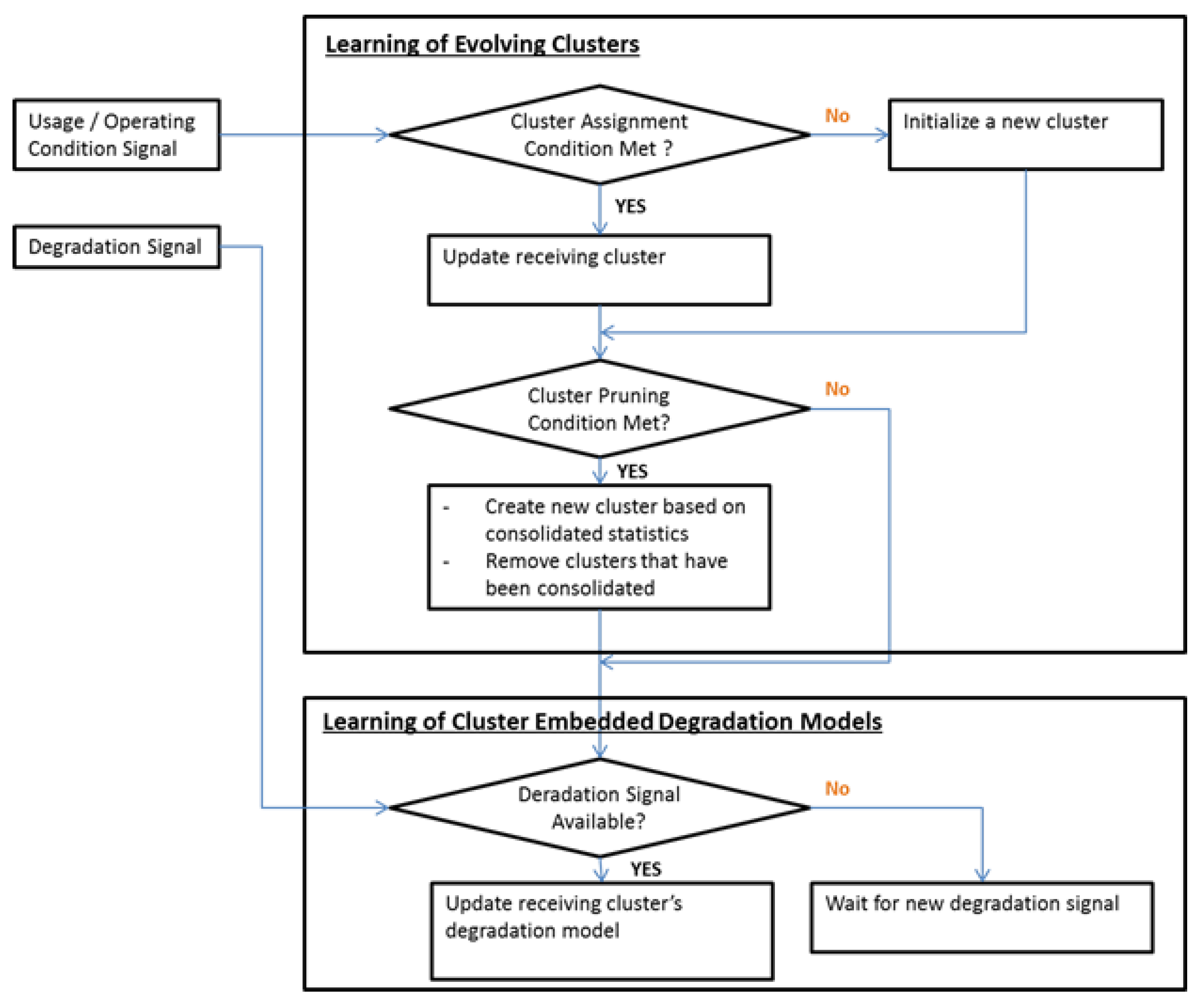
In Scheme 1, the overall integrated method’s major procedures are summarized. It is broken down into two parts. The upper part A of the flowchart focuses on the identification of the usage and operation condition through the MIRGKL clustering algorithm (cluster assignment or creation). The lower part B of the flowchart deals with the learning of cluster-specific degradation models. At the prediction phase, after a cluster has been assigned, the corresponding cluster’s local degradation function will be applied to make a prediction.

For most systems, data required for part A are typically more readily available for control and generic processing monitoring purposes. For a machine with rotational parts, they could include things, such as the RPM readings or loadings and may include temperature information from a thermocouple. From these measured signals, statistical, model-based, or expert experience-based features can be calculated. When combined with other state information, such as the on/off status or predefined operation modes, conditional usage patterns can be extracted, and trends can be obtained separately for each known state. Such predefined states can be understood as an alternative to the clusters identified by the MIRGKL algorithm. When such predefined major operating conditions are absent, unsupervised clustering algorithms, such as MIRGKL, becomes useful to identify them through continuous monitoring. In addition, if predefined operational states of the machine is available, MIRGKL can still be helpful in identifying different sub-modes for each known states if desirable (i.e., the presence of multiple/nonlinear modes of degradation). One example of such a case would be from historical data, where there may exist multiple failure patterns within the same predefined operational state, indicating that the underlying failure path may be multi-modal.

2.3. Learning Multiple Degradation Paths with MIRGKL-Plus

The lower part B of Scheme 1 separates the learning procedure of cluster-specific local models from A. Unlike part A of the flowchart, the degradation signal in part B is often not available without some definition of the progression of degradation being defined and measured with additional sensor(s) or estimation. Different alternatives exist as to obtaining indirectly inferred degradation signals. For example, the survival probability within a predefined time window can be computed from machine maintenance records where operation time to failure (OTTF) and time to repair (TTR) information are available. Another example to infer degradation information would be to expect a brand-new part or machine (inspected) to have zero or close to zero degradation. Inferred degradation would increase dramatically (i.e. over a pre-specified failure limit) when the part or machine is determined to be non-functional for its designated task. In real-world problems, intermediate degradation levels are typically determined with scheduled measurements and estimations to produce quantifiable measures of the well-being of the system that can be physically interpreted.

Because A and B of Scheme 1 are highly asynchronous, the training in part B can be either inactive or create inferred degradation information through interpolation in an effort to facilitate the learning process (requires buffering of the clustering assignment history information). Depending on how the degradation data is obtained, part B would most likely be executed in a delayed fashion with a log of cluster assignments and local models, e.g., if RUL is applied as the degradation signal and such information is unavailable until EOL (end-of-life) has been confirmed. In this situation, part B would not be executed until occurrence of an EOL event.

3. MIRGKL-Plus for Prognostics Tasks

In this section, experiments are performed on real-world case studies to study the effectiveness of the proposed MIRGKL-plus method. The case studies focus on the following two common applications in PHM: (i) drilling process, and (ii) brake wear monitoring. One should note that the formats of the RUL are different; in (i) the drilling process, the RUL is expressed as the number of additional drills the drill-bit will be able perform, which decreases as integers as the number of drilling tasks been completed, while for (ii) brake wear monitoring, the RUL is the actual brake pad thickness.

3.1. Drilling Process Application

3.1.1. Experimental Setup

The drilling process is one of the most widely applied machining processes and is chosen as the test bed for validation of the proposed autonomous prognostics framework. A HAAS VF-1 CNC Machining Center with a Kistler 9257B piezo-dynamometer (250 HZ) is used to drill holes in 1/4-inch stainless steel bars. Sensors are in place to measure the following: (1) thrust force (F), and (2) rotational torque (Q). High-speed twist drill-bits with two flutes were operated at a feed rate of 4.5 inch/minute and spindle speed at 800 rpm without coolant. An illustration of the experimental setup is shown in Figure 1. Illustration of experimental setup showing the controlled drill-bit, sequential drilling on the workpiece, rotational torque, and thrust force Figure 1, where the workpiece arrangement, holes produced after each drilling operation, drill-bit orientation, and applied thrust force and rotational torque are shown.

A drill-bit is a cutting tool to create holes by removing materials with controlled thrust force and rotational movements. Each new drill-bit was visually inspected to ensure that no visible defects were present on the unit. Once the drill process starts, it repeats the same drilling tasks multiple times until a physical failure is detected. These physical failures are typically associated with excessive wear and deformation resulting from being subjected to high temperatures during operation. During each drilling task, a dynamometer captures a thrust force and torque signal from a torque sensor in the form of time series data. While we demonstrate the effectiveness of the proposed method utilizing the drill-bit data, it should be straightforward to apply to a wide array of machine and systems in a cooperative learning setup. Due to the varieties in the natures of different systems and how they degrade and age over time, signal processing, feature extraction, and degradation signal inference designs may differ to be able to effectively identify underlying failure paths.

3.1.2. Dynamic Time Warping (DTW) Algorithm

In real-world problems, time series data from repeated measurements or data from different channels may have different sample rates, time-varying sampling rate(s), or both, which make them out of phase when pairwise comparisons need to be performed. In those situations, widely applied Euclidean distances, due to their known weakness of sensitivity to distortion in the time axis [48], may not be the best choice for such tasks. Dynamic time warping (DTW) is a distance (similarity) measure originally developed in the speed recognition community [49], which proposes a non-linear mapping procedure to minimize the difference of the time series pair of interest before computing their differences. Despite its computational complexity, the method’s ability to deal with local out-of-phase signals, improve signal alignment, and ability to deal with signals of different lengths make it the ideal algorithm to compare and derive a quantifiable measure for time series patterns in the data mining [50,51,52], bioinformatics [53], medicine and engineering communities.

Here, DTW focuses on computing the similarity between two time series, one sequence Q with length of n and another sequence C with length m, where the following is true:

$$Q=q_1,q_2,\cdots ,q_i,\cdots ,q_n$$

(11)

$$C=c_1,c_2,\cdots ,c_j,\cdots ,c_m$$

(12)

The associated warping cost is expressed as follows:

$$DTW\left(Q,C\right)=min\left\{\sqrt{{{\displaystyle \sum }}_{k=1}^K{w}_k}\right\}$$

(13)

An n-by-m matrix with the squared (Euclidean) distance between q_i and c_j is computed through (q_i–c_j)², and w_k is the matrix element (i,j)_k that belongs to the kth element of a warping path W. The optimal path is typically calculated by dynamic programming.

3.1.3. Feature Extraction of Drill-Bit Data with DTW

To demonstrate the capability of MIRGKL embedded with a survival function for prognostics purposes, we resort to conceptually simple features computed using DTW. For each drilling task of a drill-bit, the DTW computation will compute the distances of thrust force (F) and torque (Q) with respect to a pair of nominal thrust force (TF_n) and nominal torque (TQ_n) profiles conducting the same task. Essentially, the functioning features we are using are the deviations between the most current thrust force and torque profiles compared with some nominal ones. The 2-D feature vector as a result can be expressed as follows:

$$X_{T=1,2,\cdots ,t}=x_1,x_2,\cdots ,x_t$$

(14)

$$x_t=\left[DTW\left(T{F}_n,T{F}_t\right),DTW\left(T{Q}_n,T{Q}_t\right)\right]$$

(15)

It should be noted that T is the cumulative count of the number of drilling tasks conducted for the current drill-bit. The feature calculation as described in (14) and (15) takes place after the completion of a drilling task when the thrust force profile and torque profile become available to compute $DTW\left(T{F}_n,T{F}_t\right)$ and $DTW\left(T{Q}_n,T{Q}_t\right)$ according to (15). Here, $T{F}_t$ and $T{Q}_t$ are, respectively, the force and torque measures for the drill task number t. Nominal thrust force, TF_n, and nominal torque, TQ_n, are typically determined from the first few fully completed drills. For this dataset we have determined that the second drilling task for each drill-bit is to be used as the nominal profiles due to large variability among the first drilling profiles between drill-bits. This may be due to different levels of minor residues (non-visible) on each drill-bit initially; furthermore, after the first drilling task (as a conditioning step) each drill-bit was mechanically cleaned to a more similar initial condition. Because we define the nominal state to be obtained from the second drilling task, the learning and prediction procedure will actually start with the third drilling task for each drill-bit.

In Figure 2, feature calculation using DTW with thrust force (upper figure) and torque (lower figure) with multiple drill-bits are shown. Using data from the second drill task as the nominal profiles, both DTW-based features trended up as the drill-bit degrades and eventually reaches a high point after which the drill-bit no longer usable. The last feature values for each drill-bit are marked with a red star marker and the prior value is marked with a black circle. To make the outcome of the prognostic prediction from proposed algorithm more useful, we determine the RUL of the drill-bit to be close to zero for the drilling task prior to the last one, the reason being that if the last drilling were to be started, it is highly likely that the finished drilling would be deemed unsatisfactory. Therefore, the algorithm shall be able to predict if RUL is reached or is fairly close after the drill prior to the last one was completed to avoid defective parts being produced as a result of a bad drill-bit. At the high level, if a drill-bit went through six successful drills and failed at the seventh, we have the RUL back-computed similar to the following illustration:

Drill Task #1: RUL count = n/a;

Drill Task #2: RUL count = n/a (nominal drill);

Drill Task #3: RUL count = 7 − (3+1) = 3;

Drill Task #4: RUL count = 7 − (4+1) = 2;

Drill Task #5: RUL count = 7 − (5+1) = 1;

Drill Task #6: RUL count = 7 − (6+1) = 0;

Drill Task #7: RUL count = n/a.

The RUL count is a number that represents how many “good” drills are remaining for the drill-bit to produce. The last drill task’s RUL will not be available because, in the experiment, they come to a stop due to failures that are not deemed as satisfactory drills. The $RU{L}_N$ is formally defined in Section 3.1.4, but they are directionally proportional to the illustration above.

The two-dimensional DTW-based feature is applied to the MIRGKL clustering algorithm, as shown in the upper portion of Scheme 1, to identify major operating patterns as clusters that are reasonably unique when compared to one another. The following paragraph will describe in detail the determination of RUL-based normalized degradation information for the training of cluster-specific degradation models.

3.1.4. Inferred RUL Information

As described in previous paragraph, we obtain nominal profiles from the second drilling task of each drill-bit to perform DTW-based feature calculation. In addition, we define the drill prior to the last one for each drill-bit as RUL being reached to avoid additional drilling tasks being performed. As a result, the normalized RULs for the third drilling task and the drilling task prior to the last one for each drill-bit was set as follows:

$$RU{L}_N\left(D, T=3\right)=1-\epsilon ;$$

(16)

$$RU{L}_N\left(D,T=T_D-1\right)=\epsilon ;$$

(17)

Equation (16) can be regarded as providing the maximum value representative of a close to new drill-bit at the beginning; (17), on the contrary, represents when the drill-bit is almost at the end of the life. Here, ε are small values (i.e., 0.005) to avoid numerical problems during recursions. Furthermore, D represents the drill-bit number, T_D represents the total number of drills a drill-bit performed, and ε represents a small number to avoid numerical difficulties in the learning procedure of cluster-specific local models as described in (M). For the RUL_N of drills between T = 3 and T = T_D − 2, we linearly interpolate their values according to $RU{L}_N\left(D, T=3\right)$ and $RU{L}_N\left(D,T=T_D-1\right)$. This interpolation procedure enables cluster-specific local models to undergo more updates rather than a total of only two updates amongst all existing clusters during a drill-bit’s life cycle. The inferred normalized RUL of intermediate drills can be expressed through the following interpolation:

$$RU{L}_N\left(D, T\right)=1-\epsilon -\frac{1-2\epsilon }{T_D-3}\ast \left(T_D-T\right); 2<T<T_D$$

(18)

In summary, inferred normalized RUL for the nominal drill (third drill) is assigned to have a value close to 1 and the drill before the last for each drill-bit is assigned to be close to 0. From these two initial and final inferred normalized RUL values, intermediate ones were generated by linear interpolation. Since T_D will not be known until the drill-bit actually reaches its end-of-life, $RU{L}_N\left(D, T\right)$ information and subsequent cluster-specific degradation models’ updates will occur in a delayed fashion with the obtained cluster sequence buffered throughout the drilling process.

3.1.5. Initial Data Analysis

With the setup described in Section 3.1.1, total of 16 drill-bits were used in the experiment where each piece was in brand new condition with no noticeable visual imperfections. After the test, during which each drill-bit performed an identical drill task until EOL, we obtained the following information as to how many drills each drill-bit completed.

As shown in Figure 3, drill-bits #5, 6, 7, and 8 in the experiment lasted almost twice the number of total drilling tasks as all other samples. Given that the subjects of the drilling, stainless steel bars, were of the same spec, we assume this large variance in the useful life may be the result of the following factors:

• Parts (drill-bit and stainless bar) may have non-uniformity or manufacturing variations that may not be easily detectable from visual inspections
• Drilling process controls (programmed thrust force and/or torque profiles) may be close to the operational limit of the setup

However, such large variation in their degradation profiles also makes this particular set of experimental data suitable for data-driven prognostics methods based on evolvable models, such as the one we are proposing. The rationale is that the MIRGKL will identify online evolving clusters matching different groups of repeated operational patterns with local degradation models (learned in a delayed online fashion) corresponding to uniquely different degradation profiles.

With total of 16 similarly conditioned new drill-bits, a total of 443 drilling tasks were carried out. As described in Section 3.1.3, the data for the first drillings of each drill-bit were skipped due to excessive noise and, as a result, the DTW-based feature calculation using the second drilling task of each drill-bit as the nominal pattern starts from the third drilling task (self-comparison is skipped). Adding the definition of the drilling task before the last one to have the lowest assigned normalized RUL value, the number of each drill-bit’s drilling tasks being used for modeling will be reduced by three. Therefore, the original 443 drilling tasks from 16 drill-bits were reduced to 443 − 48 = 395 to validate the method.

Using the MIRGKL online clustering algorithm, a total of 33 clusters were identified with the top three most utilized clusters being #1, #2, and #11, as each experienced more than 39 (or 10% of all populations) updates from drilling patterns being assigned to them. Clusters #3, #5 ~ #10, #12, #13, #15, #16, #21, #25, and #28 ~ #33 each experienced less than five (or 1% of all populations) updates, making them candidates to be dropped off during the prediction phase due to a lack of training/significance. The total numbers of updates each of the identified 33 clusters are shown in Figure 4.

3.1.6. Setup #1—Fully Online Mode (Perfect Information)

As previously described, the inferred normalized RUL information will not become available until the drill-bit in the current experiment has reached RUL. As a result, the training of cluster-specific local model in reality would take place in a delayed manner relative to the MIRGKL clustering algorithm. However, to demonstrate the model’s performance in cases when (inferred) RUL may indeed be available enabling the local degradation model to be updated subsequent to cluster assignment, we present the DTW pattern and inferred normalized RUL information in a fashion to simulate such a scenario. In other words, for each drilling task, the DTW-based patterns is first applied to determine a cluster with the best match to predict the remaining useful life (prediction phase) or, if the closest cluster is not sufficiently close, a new cluster is created. After that, the cluster learns from the pattern by either updating an existing cluster or creating a new one. Finally, assuming the availability of inferred RUL information, the active cluster’s local degradation model learns from that in a recursive fashion. Since the overall model is updated essentially at a one sample delay, the overall performance in this setup is quite good. In Figure 5, Figure 6 and Figure 7, we observe that the predictions track the inferred RUL values very closely.

In

Table 1. Cluster assignment history of drill-bits #1 ~ #4.

	Cluster Assignment
Drilling Task #	Drill-Bit #1	Drill-Bit #2	Drill-Bit #3	Drill-Bit #4
1	*1	1	1	1
2	*2	1	1	1
3	2	1	1	1
4	2	1	1	1
5	2	2	1	1
6	*3	1	1	1
7	*4	1	1	1
8	3	2	1	11
9	*5	2	1	11
10	*6	2	1	11
11	*7	1	2	1
12	*8	*11	2	2
13	*9	1	4	1
14	9	*12	*17	2
15	*10	12	17	4
16	10	*13	17	*20
17	8	*14	17	20
18	8	12	*18	18
19		*15	*19
20		*16	16

and

Table 2. Cluster assignment history of drill-bits #5 ~ #8.

	Cluster Assignment
Drilling Task #	Drill-Bit #1	Drill-Bit #2	Drill-Bit #3	Drill-Bit #4
1	1	1	1	1
2	1	1	1	1
3	11	1	1	1
4	11	1	1	1
5	1	1	1	1
6	11	1	1	1
7	11	1	1	11
8	11	11	11	1
9	11	11	11	11
10	11	11	11	11
11	11	11	11	11
12	11	11	11	11
13	11	11	11	11
14	11	11	11	11
15	11	11	11	11
16	11	11	11	11
17	11	11	11	11
18	11	11	11	11
19	11	11	11	11
20	11	11	11	11
21	11	11	11	11
22	11	11	11	11
23	11	11	11	11
24	11	11	11	24
25	11	11	11	24
26	11	11	11	24
27	11	11	11	24
28	11	11	11	11
29		11	1	24
30		11	11	11
31		11	*24	24
32		1	1	11
33		2	1	11
34		2	1	11
35		2	11	11
36		2	1	24
37		2	1	11
38		2	11	1
39		*23	1	11
40		*23	1	1
41		19	1	1
42			1	1
43			1	1
44			11	1
45			2	1
46			20	2
47			20	24
48			20	1
49			17	26
50			*25	20
51				22
52				14

, we also show the history of cluster assignment history, where new cluster creation is marked with ∗.

Without additional processing (i.e., smoothing or averaging) of the predicted RUL values, fully online implementation of the MIRGKL with local models provides estimations closely following the inferred truth values (inferred normalized RUL). These results show that through the use of multiple learned degradation distributions, effective estimation of the RUL can be achieved even if the true underlying distributions and their quantities may be unknown.

3.1.7. Setup #2—Semi-Online Mode (Delayed Information)

In Section 3.1.6, we describe a setting where each drilling patterns comes with an inferred normalized RUL reading to demonstrate MIRGKL with embedded local functions to make a one-step-ahead prediction based on the models that are incrementally updated online. However, assuming that perfect information is made available which is aligned with clustering process is not realistic. The drill-bit experiment is a good example of such a case, because it is not possible to know the actual RUL information until actual EOL (end-of-life) has been reached. RUL information of past drilling tasks can only be labeled after failure takes place. The initial nominal normalized RUL is assigned to have a value close to 1 (1-ε) and the last drill is assigned to have a RUL close to zero ε, as shown in Section 3.1.4.

In this section, to reflect the actual timing when the inferred RUL become available, we engage in the local function update only when a drill-bit’s EOL has been reached. Before such a scenario occurs, the MIRGKL operates its clustering portion (updating, creating, and pruning) without any update made to the local degradation model from which RUL predictions are made. In other words, we introduce a variable delay in the learning of the local degradation models that is caused by the fact that each drill-bit will last somewhat different numbers of drilling tasks before they fail. This is a much more challenging setup in comparison to Section 3.1.6, but it matches closely to the real-world scenario where RUL information becomes available at EOL. That is when refinement (training) of local degradation models can take place, because the truth values of the overall process degradation become available in a usable form for the learning process.

In Figure 8 and Figure 9, in comparison to Figure 5 and Figure 6, one can see the effect when variable delays have been introduced. For the first drill-bit (first drill-bit data in Figure 8), predicted results are constant values because all clusters’ local model parameters are still default values and no update can be performed until the first drill-bit reaches its end-of-life (EOL). From drill-bit 2 and 3, prediction results started to improve slowly as each cluster’s local model started to receive additional updates. For the fifth drill-bit in Figure 9, existing clusters’ local models were not able to anticipate the significantly extended usage time (42 drilling tasks), as existing clusters’ local models were trained with data from drill-bits 1–4 that, at most, lasted 20 tasks. Nevertheless, prediction results for drill-bits 6–8 improved significantly as local models gradually adapted with data from drill-bits 5–7. The results for drill-bits 9–16, as shown in Figure 10, are largely similar to what is shown in Figure 7 (the perfect information setting in Section 3.1.6), since predictions are made from models that have already seen similar degradation profiles exhibited in drill-bits 1–4.

Figure 11 and Figure 12 (the corresponding zoomed-in view) show the degradation profile not by drill-bit but by each cluster, so we can verify if distinct degradation profiles were captured with different clusters. Clusters with at least 3% (10 updates) are shown in their individual local degradation models. Note that these clusters are not ordinal, meaning that cluster #2 does not necessarily have a longer tail than cluster #1 and a shorter tail when compared to cluster #3. By that same token, some of these degradation profiles could be similar events, though we know that, in the feature space where the clustering takes place, these clusters occupy different regions. This is interpreted as the fact that some combinations of the torque and thrust force end up having similar normalized RUL patterns at least within certain value ranges on the cumulative usage axis (cumulative number of drilling tasks performed).

In Figure 12, a zoomed-in view of Figure 11, if we were to set up the warning threshold for predicted RUL to be around 0.05, one can clearly see that degradation models can be divided into approximately 3 groups that will exceed that threshold at around 25 samples, 30 samples, and 70+ samples. The setup of such a threshold requires special care, as the value should be sufficiently large (pessimistic) such that the warning will be in time before the actual EOL is reached (a couple of drills ahead). In other words, if the threshold is set too low (too optimistic) it causes the warning to come up too late, and this may result in a higher chance of producing parts with bad drills that need to be scrapped or reworked.

3.2. Brake Wear Monitoring with MIRGKL-Plus Algorithm

Brake and tire systems are critical elements that allow the variable increments, decrements, and maintenance of propulsive forces as commanded by the driving inputs to achieve desired vehicle speed. Both of these systems are subjects to wear that may be impacted by the vehicle setup, driving patterns and their operating conditions, which is the subject of other investigations of other type of systems, where their wear and tear have even direr implications. Therefore, the ability to predict prognostics information is of critical importance [30,43,54]. With MIRGKL-plus, we are taking a more data-driven approach to the problem of brake pad wear as an example of systems with slow degradation dynamics. The benefits of taking such an approach are as follows:

• Using only existing signals from the vehicle—unlike a physics-based approach, MIRGKL-plus does not require added high rate and high-fidelity sensory information, which could have otherwise made this type of solution prohibitive in a real-world setting. For this particular experiment, we only require the access to read and store the existing signals from the CAN network and to have the pad depth be measured infrequently;
• Detailed system characterization is not needed.

Typical model-based approaches are costly, requiring detailed mathematical representation of failure processes, extensive parameter tuning, and access to laboratory collected data. With a data-driven method, less effort is required on the modeling side of the system, but more effort is needed to obtain a set of feature calculations that will have a noticeable impact on the progression and variability of various degradation processes.

3.2.1. Experiment Setup

The experiment involved five identical vehicles that entered their individual employer-sponsored management leases at different times. We chose such a setting due to the fact that these vehicles are maintained at a centralized location where infrequent but periodic measurements of the brake pad thickness are taken. Front left (FL), front right (FR), rear left (RL), and rear right (RR) brake pad measurements are taken separately with several repetitions, and the mean values of FL, FR, RL, and RR measurements are recorded during maintenance visits. Measured thickness will be the summation of the pad, backing plate, and insulator. An example of such measurements is shown in

Table 3. Example brake pad thickness measurement table.

	FDI	FDO	FPI	FPO	RDI	RDO	RPI	RPO
Top Right	17.87	17.66	18.00	17.65	15.57	15.58	15.92	15.75
Top Left	18.11	17.81	17.85	17.71	15.86	15.73	15.38	15.35
Bottom Left	18.01	17.92	17.71	17.87	15.69	15.87	15.46	15.51
Bottom Right	17.77	17.75	17.92	17.80	15.50	15.78	15.80	15.77
Average	17.94	17.79	17.76	17.66	15.66	15.74	15.64	15.60

The five participants used these test vehicles as their personal cars with varying mileages, usages, and driving road conditions. The reason we are not performing the test in a more controlled driving environment is to be able to accumulate valuable data from real-world usages where multiple pad wear patterns may present themselves. Signals are collected at 50 HZ and include brake torque request (in newton-meter), actual brake torque applied (in newton-meter), brake on and off signal, brake pedal percentage, vehicle speed (in kph), and odometer reading (in kilometers).

In Figure 13, an example of part of a CAN message recording is shown. Similar to any CAN message, each message with a unique message ID has its own dedicated encoded bits that need to be decoded to obtain the actual recorded values. This has to be carried out message by message and then sample by sample, guided by a data dictionary that defines what information each message carries and how to decode them individually. Message ID 7D represents the message for torque-related signals, message ID 415 represents the messages related to vehicle speed, and message ID 430 is associated with the odometer reading. The brake pedal percentage signal (in message ID 165, not shown in Figure 13) has known consistency issues and, as a result, this signal is not included in subsequent analysis. Note that GPS information was not included as part of the signals being collected. As a result, using such information to retrieve grade information to take out the effect of grade on the acceleration and deceleration is not possible.

Brake pad measurement for each individual participant takes place on a monthly basis. For each wheel (Front driver side or FD, front passenger side or FP, rear driver side or RD, and rear passenger side or RP), eight measurements are taken at the top right, top left, bottom right, and bottom left from both inside and outside facing angles. An example of a typical measurement record table is shown in Table 3 above. The overall data collection process lasted approximately 6 months due to resource limitations and the leasing terms.

3.2.2. Feature Extraction

In [55,56], the granulation form (interval partition for valued variables) of information representation were treated as states in Markov chain modeling. This technique captures multiple models with different context combinations allowing learned state transition patterns to be sensitive to contexts. In the case of brake data, we applied partitioning in the space spanned by speed and acceleration but without the tracking of transitions between defined granules. Instead, we obtain accumulative statistics individually for each defined partition, resulting in a granule-based braking pattern map (GBBP map) containing the conditional behaviors of each driver.

A 10 × 10 pace partitioning in terms of speed and acceleration is defined as follows:

-

Vehicle speed—0-5-10-15-25-35-45-65-85-105-120 (kilometers per hour);

-

Vehicle acceleration—0-0.05-0.1-0.2-0.3-0.5-0.75-1-1.25-1.5-1.75 (G or 9.81 m/second).

For both speed and acceleration, an additional partition (11th partition) is reserved for values exceeding either the min or max of defined regions. The 11th partition is in place to capture the full picture of the usage profile. Such information is necessary to extrapolate the usage space in the prediction phase. For example, for the same amount of 1000 km worth of driving, driver A may engage in braking actions for approximately 10 km while driver B may engage in braking actions for approximately 20 km due to variations in their driving content and each individual’s style of operation. If we were to predict the RUL for the brake pad to be the same of 100 km, meaning that we predict braking pad will reach end-of-life after braking for an additional 100 km, this would translate into different remaining driving distances because, on average, driver B brakes more per unit distance of driving. For driver A, this translate to approximately 1000 ∗ (100/10) = 10,000 km of driving distance remaining, but for driver B this would translate to only 1000 ∗ (100/20) = 5000 km of driving distance remaining.

In

Table 4. Braking distance vs. driving distance comparison among participants.

	Total Braking	Total Driving	Braking
	Distance (km)	Distance (km)	Distance %
Driver #1	876.73	14,232.24	6.16%
Driver #2	551.20	7535.11	7.32%
Driver #3	475.96	8614.74	5.52%
Driver #4	450.08	14,973.91	3.01%
Driver #5	326.14	7420.22	4.40%

above, we show the total driving distances, braking distances, and percentage of braking in total driving distances to highlight the significant variations across drivers. Among the five participants, we saw the lowest percentage of braking distance in terms of total driving distance to be around 3% for driver #4 and the highest to be 7.32% in driver #2. As a result, even if the brake wear rate was assumed to be the same in braking situations, we expect driver #2 to wear out the brake pad much faster (at least two times faster) than driver #4. If a system were to present information associated to “distance until brake pad replacement”, we believe this type of individual behavior differences has to be considered.

The resulting GBBP maps, which are re-calculated at a predefined interval (25 km), and results from the previous intervals are stored. Mainly, a total of three types of GBBP-maps are obtained, as follows:

-

Distance travelled (GBBP_Dist);

-

Deceleration (GBBP_Decel);

-

Actual toque applied (GBBP_Torq).

Out of the three GBBP maps, we calculated two features that shall intuitively capture first the preferences on the braking levels (exhibited and controlled by the driver) and secondly the braking system’s performance degradation progression over time. We defined these two features as follows:

$$X_{decel\_pref}\left(t\right)={\int }_{i=1}^{k}w\left(i,t\right)\ast \frac{GBB{P}_{Decel}\left(i,t\right)}{GBB{P}_{Dist}\left(i,t\right)}$$

(19)

$$X_{decel\_effi}\left(t\right)={\int }_{i=1}^{k}w\left(i,t\right)\ast \frac{GBB{P}_{Dist}\left(i,t\right)}{GBB{P}_{Torq}\left(i,t\right)}$$

(20)

where i denotes the unique index of the granule, w(i) stands for the normalized weight obtained from normalizing GBBP_Dist, and k represents the total number of granules being taken into consideration. In our case, although a total of 11 ∗ 11 = 121 granules are defined, only 10 ∗ 10 = 100 of them will be included in the calculation. This is because the 11th partition in both the speed and acceleration spaces contains “non-braking” driving activities and we assume no pad wear should take place in those situations.

Since brake wear is a slowly progressing phenomenon, we imposed a moving window of 6 or the equivalent of 6 ∗ 25 = 150 km as a way to filter and smooth out the information. Here, $X_{decel\_pref}$ represents a quantifiable measure as to the driver’s preference in terms of the level of deceleration during such events. For a more spirited or sporty type of braking behavior, the overall value of $X_{decel\_pref}$ will be larger relative to the value of $X_{decel\_pref}$, corresponding to a more comfortable or relaxed type of behavior. Driving content and sudden extreme conditions (i.e., crash avoidance) may skew $X_{decel\_pref}$ to various extents, and the effect of them should be minimized by the use of a moving window. Here, $X_{decel\_effi}$ represents the efficiency for the overall braking action. When the braking system is operating at high efficiency, $X_{decel\_effi}$ will have a “low” absolute value indicating unit torque achieved over a “short” breaking distance; when $X_{decel\_effi}$ is “high” in absolute value, it represents a lower efficiency for the braking system as unit torque results in a “longer” braking distance.

In the upper plot of Figure 14, it is interesting that, in the long run, despite differences in the driving content, the deceleration intensity preferences (level of deceleration per unit distance) for participating drivers remain as relatively constant values for each of the participants. This observation corresponds well with the intuition that an individual’s preference in terms of the feel of a deceleration level regulated by a driver’s control inputs is largely a personal driving attribute that does not change or evolve rapidly. On the other hand, in the lower plot of Figure 14, one should note that for all drivers, even though each individual’s deceleration preferences remain almost constant (upper plot), there are clear trends of degradation in terms of the braking systems’ performance. For drivers #1, #3 and #4, initial signs of improvement (downward trends) led to later degraded trends after they deflected at different cumulative brake mileages. For drivers #2 and #5, their trends in the lower plot of Figure 14 are rather monotonic, except for a somewhat extended flat region for driver #2.

3.2.3. Normalized Remaining Useful Life

From

Table 5. Nominal front and rear geometrical brake thickness.

	Nominal Value (mm)	Threshold Value (mm)
Geometrical Front	18.350 (FBTn)	15.175 (FBTx)
Brake Thickness
Geometrical Rear	16.150 (RBTn)	12.975 (RBTx)
Brake Thickness

, one can see that the nominal values of thickness (thickness combining pad, backing plate, and insulator) of the front and rear brakes are different. However, the minimum threshold limits are the nominal values subtracted by 1/8 inch (25.4 mm) according to specifications. With the knowledge of the above information, we can obtain the normalized remaining useful life of both front and rear brakes as follows:

$$RU{L}_{Front Brake}\left(t\right)=\frac{X_{Front Brake}\left(t\right)-FB{T}_x}{FB{T}_n-FB{T}_x}$$

(21)

$$RU{L}_{Rear Brake}\left(t\right)=\frac{X_{Rear Brake}\left(t\right)-RB{T}_x}{RB{T}_n-RB{T}_x}$$

(22)

In (21), (22), the term t represents cumulative braking distance according to our assumption of no break wear during vehicle engagement in non-braking (idle, cruise, and acceleration) activities. As a result, t increases only in the presence of a braking activity. The initial values for different participants are different because each of them started to have their data collected months after their lease started and the data collection stopped before any of the brake pads on all vehicles reached end-of-life (6 months’ worth of data). In other words, we do not have access to both near-brand-new or near-of-life types of data from this set of data.

In the experimental setup, the generic in-vehicle signals to obtain (19), (20) arrive much more frequently than the brake pad measurements used to calculate (21), (22). Although not ideal from a data alignment perspective, this would be fairly typical for systems with similar tires and brakes. This means that precise information regarding thread and brake thickness (and wear) is made available with manual measurements and will always have the variable lag for data availability. As a result, a procedure to generate artificial normalized RUL information is applied to increase the occurrence of learning opportunities of cluster-specific degradation models. Note that since the feature is extracted then filtered as described in Section 3.2.2 based on cumulative stats, the system also need to generated inferred intermediate RUL values accordingly.

In Figure 15, T(a1)–T(a3) represents times when actual measurements of the brake pad thickness were taken. The T(b1)–T(b5) values are times when the clustering procedure took place due to availability of new features based on cumulative statistics. When clustering procedures are applied, possible outcomes include cluster assignment, cluster creation, or pruning. The red dotted line at T(b1)–T(b5) represents interpolations taken with mileage information recorded at those times with measured thickness and observed at T(a1)–T(a3).

Figure 16 (x-axis: odometer) and Figure 17 (x-axis: cumulative braking distance) shows the RUL curves of the front driver side’s brake pads for all five participants. Due to the asynchronous nature between manual measurements and how features were calculated, we show the RUL calculated from actual measurements as solid dots and inferred RUL as unfilled circles, and color coded all five participants with different colors. We noted that the rate of reduction in RUL for driver #2 is 1.63% per 1000 miles driven vs. 0.67% per 1000 miles driven by driver #4. This observation can be partially explained by driver #2′s high brake distance to total driving distance ratio and the same ratio for driver #4 turned out to be the lowest. Such a relationship holds well for both front brakes but much less so for the rear brakes. Note that when compared between Figure 16 and Figure 17, one can clearly see that with cumulative braking distance, as the x-axis aligns data from all participants better. It also better demonstrates the notion of the degradation patterns from all five participants, which may be summarized by a few prototypes (Figure 17) as to all have to be individually treated (as shown in Figure 16). The main reason for cumulative braking distance being a more effective horizon for presenting brake wear data is due to the fact that, under normal vehicle usages when the brake system is assembled properly, the wear to the brake pads will be minimal.

Figure 18 conveys similar message to Figure 17 where when information when processed in a meaningful horizon, baking patterns from several drivers may be summarized as a few prototypes. One thing to note is that the clusters shown in Figure 17 and Figure 18 are slightly different because in Figure 17 the black line (driver #2) was distinct from the rest while in Figure 18 it is visible close to the blue line (driver #1)

Essentially, we are taking the effect of different ratios of braking distances to overall driving distances exhibited by different drivers, as depicted in Table 4. If we were to build models with the information as shown in Figure 17 and Figure 18, where similar degradation patterns can be clustered and learned collectively, a learning and prediction horizon matching the underlying degradation phenomenon need to be identified and taken into account appropriately.

3.2.4. Results

Initially, we set the probability at 0.95; for two-dimensional data, this corresponds to a threshold value for chi-square statistics is 5.9915. With the features as described in Section 3.2.2, it produced an unexpected result in terms of the clusters that were identified. In this setting, as shown in

Table 6. Log of data sequence, cluster assignment, and driver identification number with probability threshold set at 0.95.

Data#	Cluster#	Driver#	Data#	Cluster#	Driver#
1	1	1	19	1	1
2	1	1	20	3	3
3	1	1	21	3	3
4	1	1	22	3	3
5	2	4	23	1	1
6	3	3	24	1	1
7	3	3	25	1	1
8	3	3	26	1	1
9	1	1	27	2	4
10	1	1	28	4	2
11	1	1	29	4	2
12	2	4	30	4	2
13	2	4	31	4	2
14	2	4	32	4	2
15	2	4	33	5	5
16	1	1	34	5	5
17	1	1	35	5	5
18	1	1

, five clusters correspond to the five participating drivers. One thing to note is that we arranged the data by the time of measurement taken, as they correspond to the time data becoming available to the system and subject to processing. Since driver numbers were assigned by each driver’s name in alphabetical order and cluster numbers are assigned at the time when it is created, in Table 6 cluster #4 matches driver #2, cluster #2 matches driver #4, and drivers #1, #3, and #5 match cluster #1, #3, and #5, respectively.

In the ideal setting where a large number of the same type of vehicles’ data are being collected, we expect the model to be able to summarize drivers with similar patterns into the same cluster. In other words, the number of prototypical patterns as represented by identified clusters should be smaller than the total number of individuals that formed the crowd or participating drivers. As drivers belonging to the same cluster incrementally contribute to the cluster-specific model, the model can be trained at the accelerated pace with respect to a portion of the population (belongs to the same cluster) for predictive purposes. To test this notion, even though we only have total of five participants, we tightened the probability threshold to an extremely high value of 0.999 to limit its criteria to create new clusters. In

Table 7. Log of cluster assignment and driver identification number with probability threshold set at 0.999.

Data#	Cluster#	Driver#	Data#	Cluster#	Driver#
1	1	1	19	1	1
2	1	1	20	3	3
3	1	1	21	3	3
4	1	1	22	3	3
5	2	4	23	1	1
6	3	3	24	1	1
7	3	3	25	1	1
8	3	3	26	1	1
9	1	1	27	2	4
10	1	1	28	2	2
11	1	1	29	2	2
12	2	4	30	2	2
13	2	4	31	2	2
14	2	4	32	2	2
15	2	4	33	2	5
16	1	1	34	2	5
17	1	1	35	2	5
18	1	1

, one can see that in this setting driver #2, #4, and #5 are grouped as one cluster in cluster #2, and that driver #1 and driver #3 continued to have clusters of their own.

In

Table 8. Mean square error for each driver, each driver’s individual brakes, and overall values with probability threshold at 0.999.

Probability Threshold: 0.999
Driver#1 FD	Driver#1 FP	Driver#1 RD	Driver#1 RP	Driver#1 Overall
0.0062	0.0056	0.0059	0.0052	0.0057
Driver#2 FD	Driver#2 FP	Driver#2 RD	Driver#2 RP	Driver#2 Overall
0.0027	0.0015	0.002	0.0031	0.0023
Driver#3 FD	Driver#3 FP	Driver#3 RD	Driver#3 RP	Driver#3 Overall
0.0202	0.0211	0.0179	0.0171	0.0191
Driver#4 FD	Driver#4 FP	Driver#4 RD	Driver#4 RP	Driver#4 Overall
0.018	0.0188	0.0158	0.0167	0.0173
Driver#5 FD	Driver#5 FP	Driver#5 RD	Driver#5 RP	Driver#5 Overall
0.00048	0.0003	0.00063	0.00057	0.000495
				Overall
				0.0086

, we summarize the performance in terms of mean square error for each driver, each driver’s individual brakes, and the overall values of all drivers. When studied together with

Table 9. Mean square error for each driver, each driver’s individual brakes, and overall values with probability threshold at 0.999.

Probability Threshold: 0.95
Driver#1 FD	Driver#1 FP	Driver#1 RD	Driver#1 RP	Driver#1 Overall
0.0062	0.0056	0.0059	0.0052	0.0057
Driver#2 FD	Driver#2 FP	Driver#2 RD	Driver#2 RP	Driver#2 Overall
0.0067	0.0084	0.0059	0.0058	0.0067
Driver#3 FD	Driver#3 FP	Driver#3 RD	Driver#3 RP	Driver#3 Overall
0.0202	0.0211	0.0177	0.0145	0.0184
Driver#4 FD	Driver#4 FP	Driver#4 RD	Driver#4 RP	Driver#4 Overall
0.0175	0.0186	0.0154	0.0164	0.017
Driver#5 FD	Driver#5 FP	Driver#5 RD	Driver#5 RP	Driver#5 Overall
0.026	0.0272	0.0219	0.023	0.0245
				Overall
				0.0117

where the probability threshold was set at 0.95, one can see that, with a tighter probability threshold, although fewer clusters (a total of three) were created, the algorithm shows a good capability to generalize information, and produced a better MSE over 26% lower than the setting that created more clusters (a total of five).

Finally, Figure 19, Figure 20, Figure 21, Figure 22 and Figure 23 show that from driver #1 to driver #5, the observed and predicted RUL of their four brakes’ (front driver side, front passenger side, rear driver side, and rear passenger side) inferred normalized brake pad thickness versus predicted value in a one-step-ahead prediction setup. These results are generated with the probability threshold set to be 0.999 when three clusters are formed to collectively learn and predict RUL profiles.

4. Conclusions

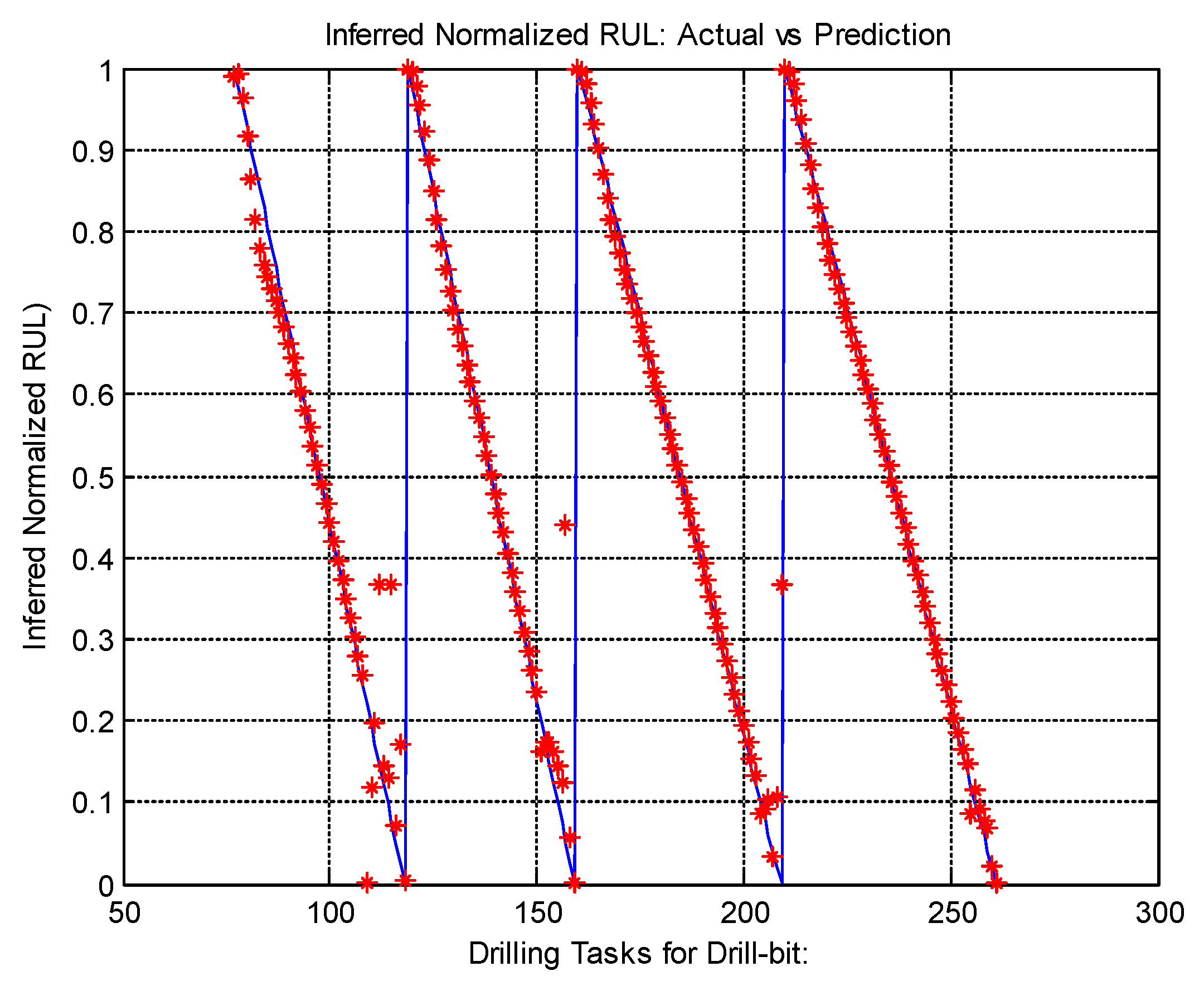
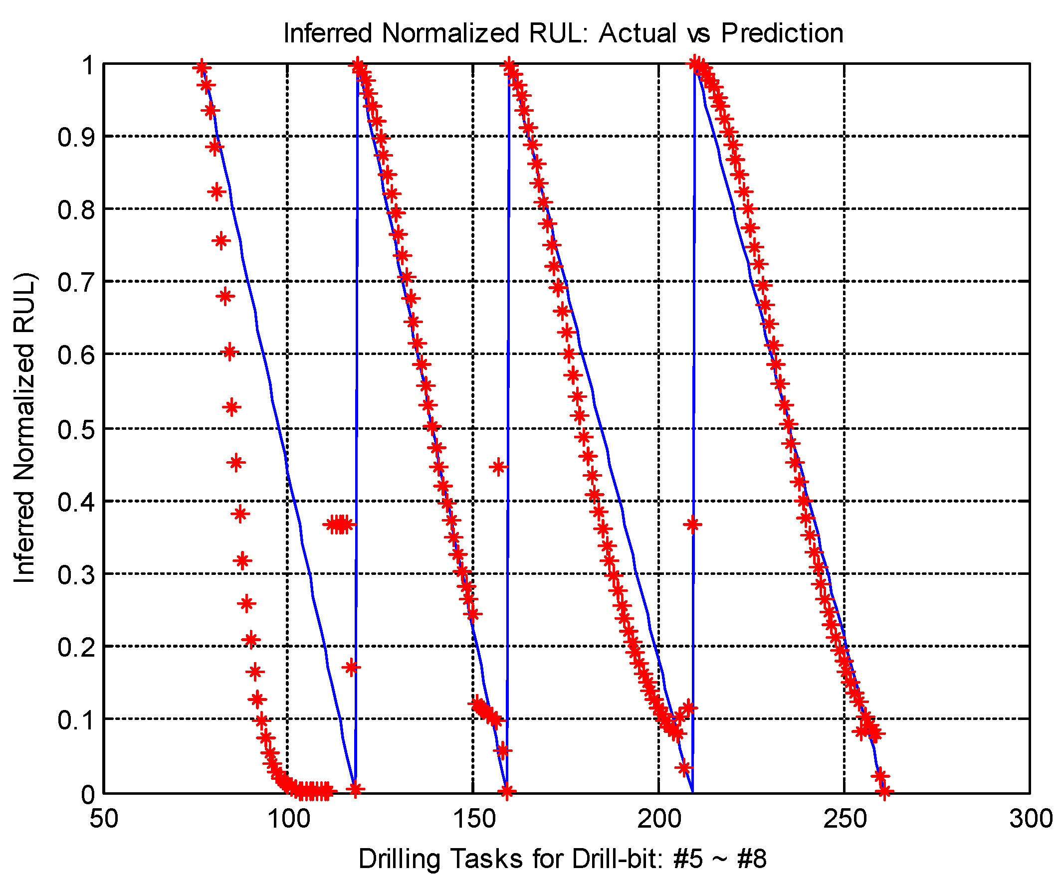
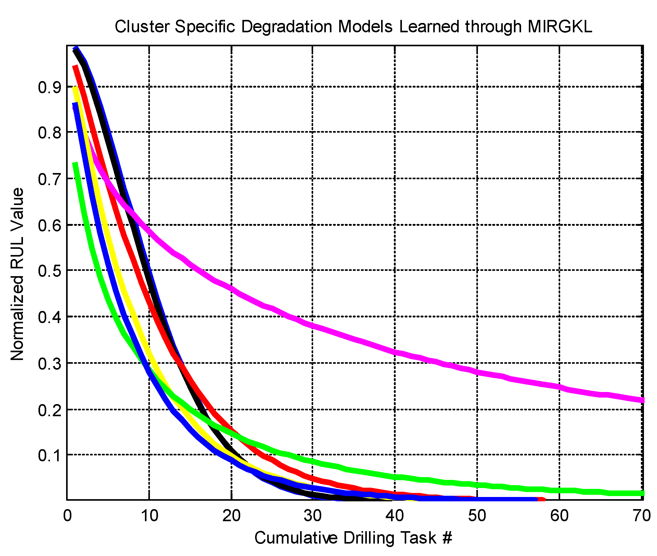
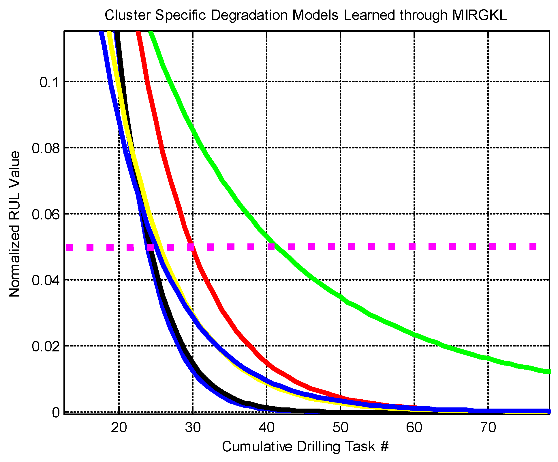
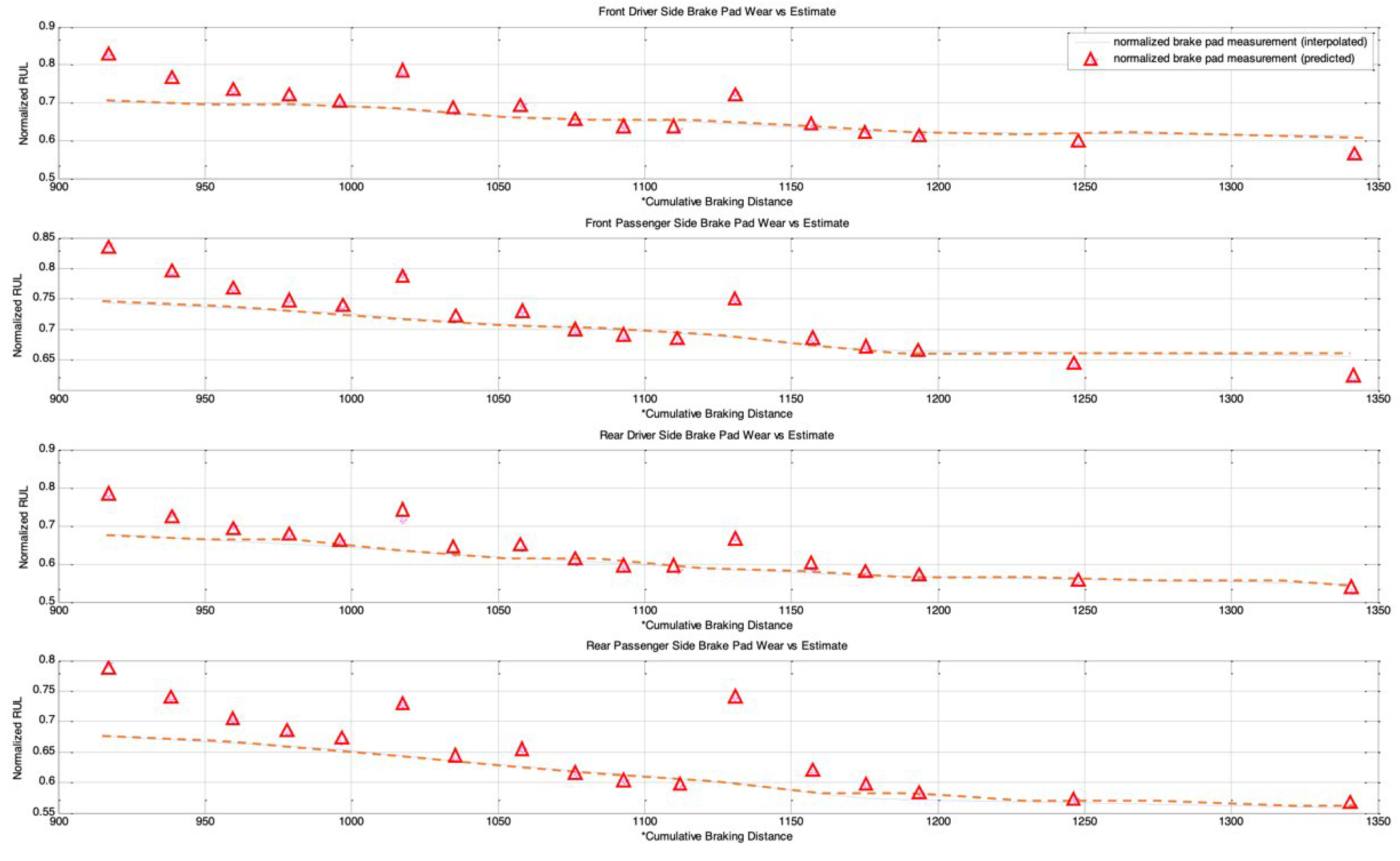
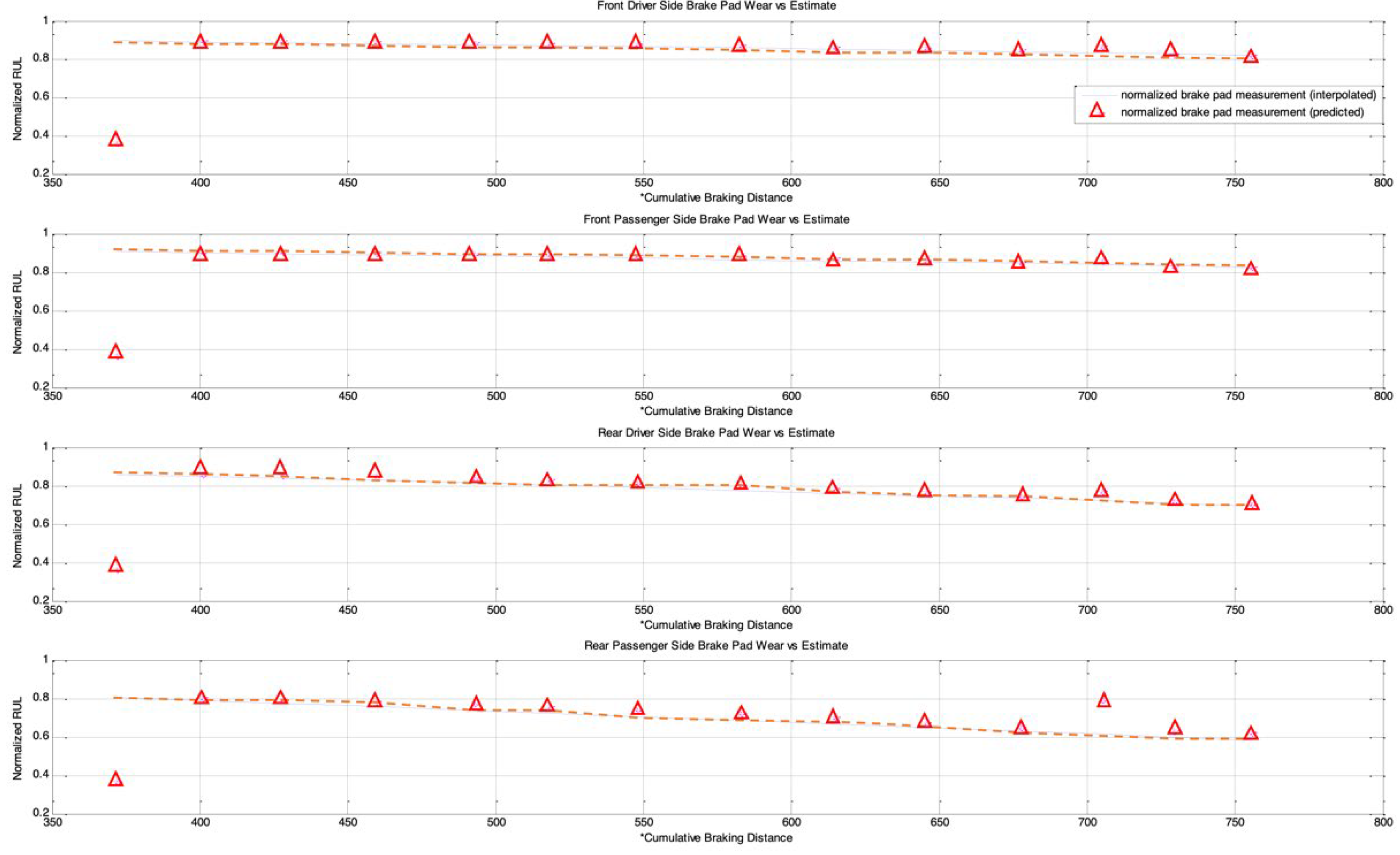
In this paper, we introduced a novel MIRGKL-plus method (MIRGLK embedded with local functions) for the prognostics of common RUL problems. We demonstrate the effectiveness of the proposed prognostic framework with the same generic local function formulation through extensive experiments with two different applications. First, the drill-bit data was obtained in a controlled experimental setting with similar brand-new conditions to determine if the number of successful drilling tasks for different drill-bits could be predicted. Second, the brake wear data was obtained from a fleet of vehicles in the field with variable initial states to determine if the brake wear could be predicted for different vehicles with different usages and driving styles. For prognostic purposes, they present significant challenges that can be summarized as follows: (1) Physical representation of the system with high enough precision for a prognostics purpose is difficult to obtain. From this perspective, we wanted to see if different simplified local models can effectively perform the learning and prediction tasks; (2) Large piece-to-piece variations cannot be well explained or tracked once experiments have been completed and with different initial states. From this perspective, we wanted to see if the proposed evolving cluster approach result in meaningful number of clusters that effectively generalizes population-level variations and behaviors; (3) Multiple underlying degradation modes may be present; (4) During the life of each test subject, the models have access to limited and infrequent observability to determine the actual degradation level. Case studies demonstrated that the proposed prognostic model was able to address the aforementioned problems and provide accurate prognostic predictions.

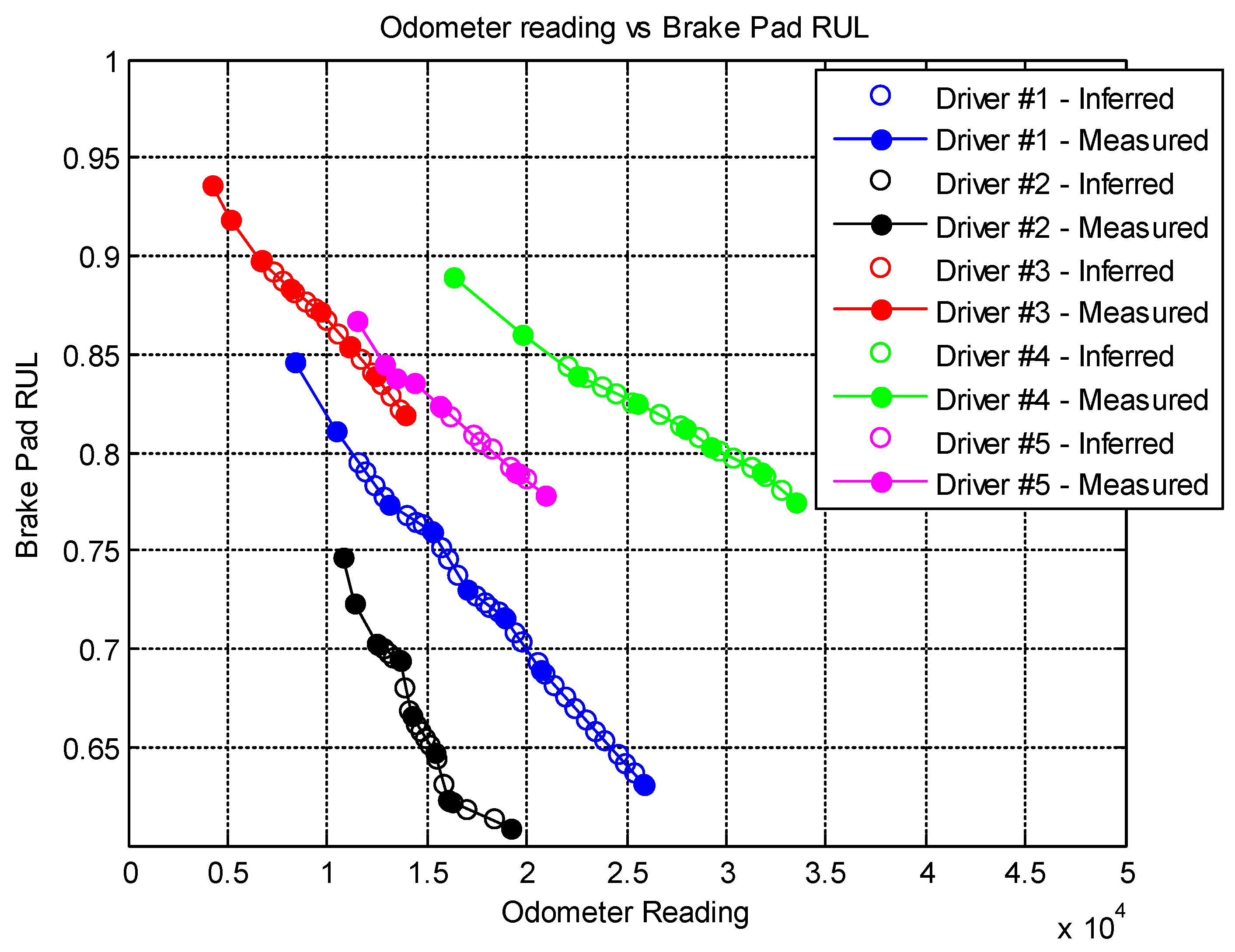
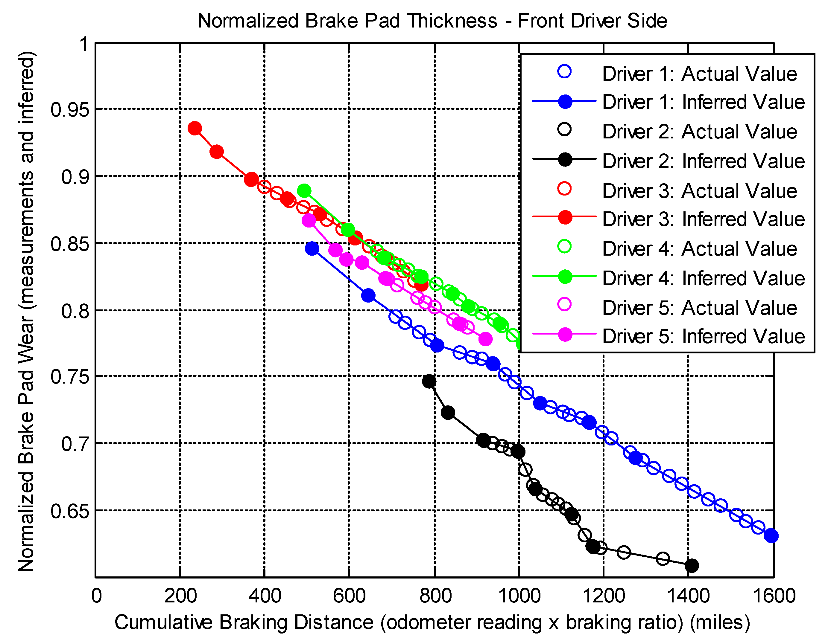
Both case studies clearly demonstrated the applicability of an evolving clustering algorithm to systems of the same type under somewhat different usage patterns. The proposed model effectively separates the data streams into groups (clusters) where different degradation patterns can be extracted for RUL prediction purposes. We have also proposed the use of limited degradation information that arrives at a different rate when compared to the generic signals. This is achieved with the use of clustering results coupled with linear interpolation and normalization of the operation limits of the crucial system parameter. Aligned normalized degradation through inference allows cluster-specific local models to be updated along with the update procedure of the overall clustering process. In the brake wear example, one thing to note is that the degradation (inferred normalized brake thickness) has to be presented in a meaningful horizon (cumulative braking distance) in order to observe and obtain meaningful results. Even though some drivers may exhibit a similar rate of wear in the horizon of cumulative braking distance, the final odometer value is where the limit may differ significantly due to their differences in braking/driving ratios, which is an aggregate of individual driving content and behavior.

Future research on the evolving clustering method and applications to investigate will be focused on the following:

A.

Improvement to MIRGKL clustering algorithm.

• Refinement to cluster merging and division mechanisms;
• Online tracking and continual characterization of both individual and overall clustering progression as additional means for process prognostics.

B.

Applications to user and behavior prognostics;

C.

Transfer learning and federated learning to improve cold/initial start issues.

For direction A, the focus will be to further devise and develop the MIRGKL algorithms, as this is key to its application not only for RUL estimation but also as a tool for auto-labeling data streams with partial labels. For B, in user related applications, we foresee that this method can be applicable to the extraction and learning of user preferences and intents and their progression during different usage horizons. One example would be a driver’s intent to take a break from driving or to refill the vehicle. This type of learning and prediction process can be facilitated with a similar hypothesis and interpolation procedure to the one shown in Section 3.2, with limited need to engage users to create the labels themselves all the time, which can be viewed as inconvenient and intrusive. Direction C points out an important aspect of leveraging many users’ data to create and update a base model, as suggested in federated learning [57]. Because MIRGKL-plus is inherently a linear combiner model, similar computes can be performed without losing its original interpretability and, if the choice of the local model is also linear, we would expect the combined model to be fairly stable. Having a base model has several implications for ML models. First of all, it can help to alleviate the cold start issues common in all ML methods. Similar to few-shot learning, a system can have all users start out with an average preference and behavior model to evolve with user’s own data over time. Secondly, for applications that have safety implications, the base model may need to be the acting model all the time, meaning that it will be the updated “base” but not the personal version of the model to be active for each user.

References

1. Lee, J.; Wu, F.; Zhao, W.; Ghaffari, M.; Liao, L.; Siegel, D. Prognostics and health management design for rotary machinery systems—Reviews, methodology and applications. Mech. Syst. Signal Processing 2014, 42, 314–334. [Google Scholar] [CrossRef]
2. Dalzochio, J.; Kunst, R.; Pignaton, E.; Binotto, A.; Sanyal, S.; Favilla, J.; Barbosa, J. Machine learning and reasoning for predictive maintenance in Industry 4.0: Current status and challenges. Comput. Ind. 2020, 123, 103298. [Google Scholar] [CrossRef]
3. Duchi, J. Derivations for Linear Algebra and Optimization; Stanford University: Berkeley, CA, USA, 2007. [Google Scholar]
4. Jain, A.K.; Murty, N.M.; Flynn, P.J. Data clustering: A review. ACM Comput. Surv. 1999, 31, 264–323. [Google Scholar] [CrossRef]
5. Xu, R.; Wunsch, D. Survey of clustering algorithms. IEEE Trans. Neural Netw. 2005, 16, 645–678. [Google Scholar] [CrossRef] [Green Version]
6. Bezdek, J.C.; Ehrlich, R.; Full, W. FCM: The fuzzy c-means clustering algorithm. Comput. Geosci. 1984, 10, 191–203. [Google Scholar] [CrossRef]
7. Hartigan, J.A.; Wong, M.A. Algorithm AS 136: A k-means clustering algorithm. J. R. Stat. Soc. Ser. C 1979, 28, 100–108. [Google Scholar] [CrossRef]
8. Yager, R.; Filev, D. Approximate clustering via the mountain method. IEEE Trans. Syst. Man. Cybern. 1994, 24, 1279–1284. [Google Scholar] [CrossRef]
9. Ester, M.; Kriegel, H.P.; Sander, J.; Xu, X. A density-based algorithm for discovering clusters in large spatial databases with noise. In Proceedings of the KDD, Portland, OR, USA, 2–4 August 1996; Volume 96, pp. 226–231. [Google Scholar]
10. Filev, D.; Georgieva, O. An Extended Version of the Gustafson-Kessel Algorithm for Evolving Data Stream Clustering. In Evolving Intelligent Systems: Methodology and Applications; IEEE Press Series on Computational Intelligence; John Wiley & Sons, Inc.: Hoboken, NJ, USA, 2010; pp. 273–299. [Google Scholar] [CrossRef]
11. Serir, L.; Ramasso, E.; Zerhouni, N. Evidential evolving Gustafson–Kessel algorithm for online data streams partitioning using belief function theory. Int. J. Approx. Reason. 2012, 53, 747–768. [Google Scholar] [CrossRef]
12. Tefaj, E.; Kasneci, G.; Rosenstiel, W.; Bogdan, M. Bayesian online clustering of eye movement data. In Proceedings of the Symposium on Eye Tracking Research and Applications, Santa Barbara, CA, USA, 28–30 March 2012; pp. 285–288. [Google Scholar]
13. Ahmed, H.; Mahanta, P.; Bhattacharyya, D.; Kalita, J.K. GERC: Tree Based Clustering for Gene Expression Data. In Proceedings of the 2011 IEEE 11th International Conference on Bioinformatics and Bioengineering 2011, Taichung, Taiwan, 24–26 October 2011; pp. 299–302. [Google Scholar] [CrossRef]
14. Dovzan, D.; Škrjanc, I. Recursive clustering based on a Gustafson–Kessel algorithm. Evol. Syst. 2010, 2, 15–24. [Google Scholar] [CrossRef]
15. Lughofer, E.D. FLEXFIS: A Robust Incremental Learning Approach for Evolving Takagi–Sugeno Fuzzy Models. IEEE Trans. Fuzzy Syst. 2008, 16, 1393–1410. [Google Scholar] [CrossRef]
16. Kavianpour, M.; Ramezani, A.; Beheshti, M.T. A class alignment method based on graph convolution neural network for bearing fault diagnosis in presence of missing data and changing working conditions. Measurement 2022, 199, 111536. [Google Scholar] [CrossRef]
17. Wang, L.; Cao, H.; Xu, H.; Liu, H. A gated graph convolutional network with multi-sensor signals for remaining useful life prediction. Knowl. Based Syst. 2022, 252, 109340. [Google Scholar] [CrossRef]
18. Li, T.; Zhou, Z.; Li, S.; Sun, C.; Yan, R.; Chen, X. The emerging graph neural networks for intelligent fault diagnostics and prognostics: A guideline and a benchmark study. Mech. Syst. Signal Process. 2021, 168, 108653. [Google Scholar] [CrossRef]
19. Caceres, J.; Gonzalez, D.; Zhou, T.; Droguett, E.L. A probabilistic Bayesian recurrent neural network for remaining useful life prognostics considering epistemic and aleatory uncertainties. Struct. Control Health Monit. 2021, 28, e2811. [Google Scholar] [CrossRef]
20. Yan, S.; Shao, H.; Xiao, Y.; Zhou, J.; Xu, Y.; Wan, J. Semi-supervised fault diagnosis of machinery using LPS-DGAT under speed fluctuation and extremely low labeled rates. Adv. Eng. Inform. 2022, 53, 101648. [Google Scholar] [CrossRef]
21. Yan, S.; Shao, H.; Xiao, Y.; Liu, B.; Wan, J. Hybrid robust convolutional autoencoder for unsupervised anomaly detection of machine tools under noises. Robot. Comput. Manuf. 2023, 79, 102441. [Google Scholar] [CrossRef]
22. Kowdiki, M.; Khaparde, A. Automatic hand gesture recognition using hybrid meta-heuristic-based feature selection and classification with Dynamic Time Warping. Comput. Sci. Rev. 2020, 39, 100320. [Google Scholar] [CrossRef]
23. Yao, S.; Kang, Q.; Zhou, M.; Rawa, M.J.; Abusorrah, A. A survey of transfer learning for machinery diagnostics and prognostics. Artif. Intell. Rev. 2022, 1–52. [Google Scholar] [CrossRef]
24. Soleimani, M.; Campean, F.; Neagu, D. Diagnostics and prognostics for complex systems: A review of methods and challenges. Qual. Reliab. Eng. Int. 2021, 37, 3746–3778. [Google Scholar] [CrossRef]
25. Catelani, M.; Ciani, L.; Fantacci, R.; Patrizi, G.; Picano, B. Remaining Useful Life Estimation for Prognostics of Lithium-Ion Batteries Based on Recurrent Neural Network. IEEE Trans. Instrum. Meas. 2021, 70, 1–11. [Google Scholar] [CrossRef]
26. Wadhera, T.; Kakkar, D.; Rani, R. Behavioral Modeling Using Deep Neural Network Framework for ASD Diagnosis and Prognosis. In Emerging Technologies for Healthcare: Internet of Things and Deep Learning Models; John Wiley & Sons, Inc.: Hoboken, NJ, USA, 2021; pp. 279–298. [Google Scholar] [CrossRef]
27. Mirbabaie, M.; Stieglitz, S.; Frick, N.R.J. Artificial intelligence in disease diagnostics: A critical review and classification on the current state of research guiding future direction. Health Technol. 2021, 11, 693–731. [Google Scholar] [CrossRef]
28. Wang, Y.; Yao, Q.; Kwok, J.T.; Ni, L.M. Generalizing from a few examples: A survey on few-shot learning. ACM Comput. Surv. 2020, 53, 1–34. [Google Scholar] [CrossRef]
29. Johansson, C.; Bergkvist, M.; Geysen, D.; De Somer, O.; Lavesson, N.; Vanhoudt, D. Operational Demand Forecasting In District Heating Systems Using Ensembles Of Online Machine Learning Algorithms. Energy Procedia 2017, 116, 208–216. [Google Scholar] [CrossRef]
30. Coble, J.; Ramuhalli, P.; Bond, L.; Hines, J.W.; Upadhyaya, B. A Review of Prognostics and Health Management Applications in Nuclear Power Plants. Int. J. Progn. Health Manag. 2015, 6. [Google Scholar] [CrossRef]
31. Huynh, K.T.; Grall, A.; Berenguer, C. A Parametric Predictive Maintenance Decision-Making Framework Considering Improved System Health Prognosis Precision. IEEE Trans. Reliab. 2018, 68, 375–396. [Google Scholar] [CrossRef] [Green Version]
32. Nuhic, A.; Terzimehic, T.; Soczka-Guth, T.; Buchholz, M.; Dietmayer, K. Health diagnosis and remaining useful life prognostics of lithium-ion batteries using data-driven methods. J. Power Sources 2013, 239, 680–688. [Google Scholar] [CrossRef]
33. Baraldi, P.; Mangili, F.; Zio, E. A Kalman Filter-Based Ensemble Approach With Application to Turbine Creep Prognostics. IEEE Trans. Reliab. 2012, 61, 966–977. [Google Scholar] [CrossRef]
34. Jia, F.; Lei, Y.; Lin, J.; Zhou, X.; Lu, N. Deep neural networks: A promising tool for fault characteristic mining and intelligent diagnosis of rotating machinery with massive data. Mech. Syst. Signal Process. 2016, 72–73, 303–315. [Google Scholar] [CrossRef]
35. Bukhsh, Z.A.; Saeed, A.; Stipanovic, I.; Doree, A.G. Predictive maintenance using tree-based classification techniques: A case of railway switches. Transp. Res. Part C Emerg. Technol. 2019, 101, 35–54. [Google Scholar] [CrossRef]
36. Kaparthi, S.; Bumblauskas, D. Designing predictive maintenance systems using decision tree-based machine learning techniques. Int. J. Qual. Reliab. Manag. 2020, 37, 659–686. [Google Scholar] [CrossRef]
37. Tseng, F.; Filev, D.; Chinnam, R.B. A mutual information based online evolving clustering approach and its applications. Evol. Syst. 2017, 8, 179–191. [Google Scholar] [CrossRef]
38. Georgieva, O.; Filev, D.P. Gustafson-kessel algorithm for evolving data stream clustering. In Proceedings of the International Conference on Computer Systems and Technologies and Workshop for PhD Students in Computing; Association for Computing Machinery: New York, NY, USA, 2009; p. 62. [Google Scholar]
39. Chenaghlou, M.; Moshtaghi, M.; Leckie, C.; Salehi, M. Online Clustering for Evolving Data Streams with Online Anomaly Detection. In Proceedings of the Pacific-Asia Conference on Knowledge Discovery and Data Mining, Melbourne, Australia, 3–6 June 2018; pp. 508–521. [Google Scholar] [CrossRef]
40. Škrjanc, I.; Iglesias, J.A.; Sanchis, A.; Leite, D.; Lughofer, E.; Gomide, F. Evolving fuzzy and neuro-fuzzy approaches in clustering, regression, identification, and classification: A Survey. Inf. Sci. 2019, 490, 344–368. [Google Scholar] [CrossRef]
41. Angelov, P.P.; Filev, D.P. An approach to online identification of Takagi-Sugeno fuzzy models. IEEE Transactions on Systems, Man, and Cybernetics, Part B (Cybernetics). 30 January 2004. Volume 34, pp. 484–498. Available online: https://ieeexplore.ieee.org/xpl/RecentIssue.jsp?punumber=3477 (accessed on 8 September 2022).
42. Keogh, E.; Kasetty, S. On the Need for Time Series Data Mining Benchmarks: A Survey and Empirical Demonstration. Data Min. Knowl. Discov. 2003, 7, 349–371. [Google Scholar] [CrossRef]
43. Bebbington, M.; Lai, C.-D.; Wellington, M.; Zitikis, R. The discrete additive Weibull distribution: A bathtub-shaped hazard for discontinuous failure data. Reliab. Eng. Syst. Saf. 2012, 106, 37–44. [Google Scholar] [CrossRef]
44. Cordeiro, G.M.; Lemonte, A.J. On the Marshall–Olkin extended Weibull distribution. Stat. Pap. 2012, 54, 333–353. [Google Scholar] [CrossRef]
45. Almalki, S.J.; Nadarajah, S. Modifications of the Weibull distribution: A review. Reliab. Eng. Syst. Saf. 2013, 124, 32–55. [Google Scholar] [CrossRef]
46. Neuner, S.; Albrecht, A.; Cullmann, D.; Engels, F.; Griess, V.C.; Hahn, W.A.; Hanewinkel, M.; Härtl, F.; Kölling, C.; Staupendahl, K.; et al. Survival of Norway spruce remains higher in mixed stands under a dryer and warmer climate. Glob. Chang. Biol. 2015, 21, 935–946. [Google Scholar] [CrossRef] [Green Version]
47. Urrutia, J.; Gayo, W.S.; Bautista, L.A.; Baccay, E.B. Survival Analysis of Patients with End Stage Renal Disease. In Journal of Physics: Conference Series; IOP Publishing Ltd.: Bristol, UK, 2015; Volume 622. [Google Scholar] [CrossRef] [Green Version]
48. Keogh, E.; Ratanamahatana, C.A. Exact indexing of dynamic time warping. Knowl. Inf. Syst. 2005, 7, 358–386. [Google Scholar] [CrossRef]
49. Sakoe, H.; Chiba, S. Dynamic programming algorithm optimization for spoken word recognition. In IEEE Transactions on Acoustics, Speech, and Signal Processing; IEEE: New York, NY, USA, 1978; Volume 26, pp. 43–49. [Google Scholar] [CrossRef] [Green Version]
50. Keogh, E.J.; Pazzani, M.J. Scaling up dynamic time warping for datamining applications. In Proceedings of the Sixth ACM SIGKDD International Conference on Knowledge Discovery and Data Mining, Boston, MA, USA, 20–23 August 2000; pp. 285–289. [Google Scholar]
51. Ding, H.; Trajcevski, G.; Scheuermann, P.; Wang, X.; Keogh, E. Querying and mining of time series data: Experimental comparison of representations and distance measures. Proc. VLDB Endow. 2008, 1, 1542–1552. [Google Scholar] [CrossRef] [Green Version]
52. Rakthanmanon, T.; Campana, B.; Mueen, A.; Batista, G.; Westover, B.; Zhu, Q.; Zakaria, J.; Keogh, E. Searching and mining trillions of time series subsequences under dynamic time warping. In Proceedings of the 18th ACM SIGKDD International Conference on Knowledge Discovery and Data Mining, Beijing, China, 12–16 August 2012; pp. 262–270. [Google Scholar]
53. Aach, J.; Church, G.M. Aligning gene expression time series with time warping algorithms. Bioinformatics 2001, 17, 495–508. [Google Scholar] [CrossRef] [Green Version]
54. Wood, A.R.; The Electronic Medical Records and Genomics (eMERGE) Consortium; Esko, T.; Yang, J.; Vedantam, S.; Pers, T.H.; Gustafsson, S.; Chu, A.Y.; Estrada, K.; Luan, J.; et al. Defining the role of common variation in the genomic and biological architecture of adult human height. Nat. Genet. 2014, 46, 1173–1186. [Google Scholar] [CrossRef] [PubMed] [Green Version]
55. Filev, D.P.; Kolmanovsky, I. Generalized Markov Models for Real-Time Modeling of Continuous Systems. IEEE Trans. Fuzzy Syst. 2013, 22, 983–998. [Google Scholar] [CrossRef]
56. Filev, D.; Kolmanovsky, I.; Yager, R. Developing Fuzzy State Models as Markov Chain Models with Fuzzy Encoding. In Fifty Years of Fuzzy Logic and Its Applications; Springer: Berlin/Heidelberg, Germany, 2015; pp. 79–106. [Google Scholar] [CrossRef]
57. Yi, J.; Wu, F.; Wu, C.; Liu, R.; Sun, G.; Xie, X. Efficient-fedrec: Efficient federated learning framework for privacy-preserving news recommendation. arXiv 2021, arXiv:2109.05446. [Google Scholar]
Scheme 1. Flowchart of evolving clustering with embedded local (survival/degradation) functions for system prognostics.
Machines 11 00040 sch001
Figure 1. Illustration of experimental setup showing the controlled drill-bit, sequential drilling on the workpiece, rotational torque, and thrust force.
Machines 11 00040 g001
Figure 2. Feature calculation using dynamic time warping (DTW) with thrust Force (upper figure) and torque (lower figure) with multiple drill-bits. Blue lines represent drill-bits which lasted less than 30 drilling tasks, and pink lines represent those which lasted more than 30 drilling tasks. Red stars indicate the instance of failure (x-axis: drilling task number) or the last drill task a drill bit undertook but failed.
Machines 11 00040 g002
Figure 3. x-axis: Drill-bit # is an unique identification number for each drill-bit used in the experiment. There are total of 16 drill-bits so they are marked as 1 – 16 accordingly. y-axis: total number of drilling tasks completed for each of the 16 drill-bit in the experiment.
Machines 11 00040 g003
Figure 4. Population of each cluster identified by the MIRGKL algorithm.
Machines 11 00040 g004
Figure 5. Normalized inferred RUL (blue line) vs. predicted RUL (red dotted line) for drill-bits #1 ~ #4.
Machines 11 00040 g005
Figure 6. Normalized inferred RUL (blue line) vs. predicted RUL (red dotted line) for drill-bits #5 ~ #8.
Machines 11 00040 g006
Figure 7. Normalized inferred RUL (blue line) vs. predicted RUL (red dotted line) for drill-bits #9~#16.
Machines 11 00040 g007
Figure 8. Normalized inferred RUL (blue line) vs. predicted RUL (red dotted line) for drill-bits #1~#4 in a delayed online setup.
Machines 11 00040 g008
Figure 9. Normalized inferred RUL (blue line) vs. predicted RUL (red dotted line) for drill-bits #5~#8 in a delayed online setup.
Machines 11 00040 g009
Figure 10. Normalized inferred RUL vs. predicted RUL for drill-bits #9~#16 in a delayed online setup.
Machines 11 00040 g010
Figure 11. Learned cluster-specific degradation models of clusters with 3% (10 points) of all data points. Each color represents one specific cluster’s learned degradation profile.
Machines 11 00040 g011
Figure 12. Zoom-in view of Figure 11. Each color represents one specific cluster’s learned degradation profile. Pink dotted line is the threshold for RUL prediction.
Machines 11 00040 g012
Figure 13. Example CAN messages recorded from a vehicle containing time stamp, message ID, and hexadecimal encoded data.
Machines 11 00040 g013
Figure 14. Upper plot shows X d e c e l _ p r e f , which is the first type of deceleration attribute. Lower plot shows X d e c e l _ e f f i (lower) which is the second type of deceleration attribute.
Machines 11 00040 g014
Figure 15. Example of the timeline of events of data upload, clustering triggered by features calculated from cumulative statistics and interpolated through inferred RUL.
Machines 11 00040 g015
Figure 16. Measured (solid dots) and inferred (unfilled circles) RUL of front driver’s side brake pad thickness.
Machines 11 00040 g016
Figure 17. Measured (solid dots) and inferred (unfilled circles) RUL of front driver’s side brake pad thickness against cumulative braking distance as the x-axis.
Machines 11 00040 g017
Figure 18. Measured (solid dots) and inferred (unfilled circles) RUL of front driver’s side brake pad thickness against cumulative braking distance as the x-axis.
Machines 11 00040 g018
Figure 19. Driver #1, inferred normalized brake wear (dashed-line) vs. predicted brake wear (triangle). Top–bottom shows front driver side, front passenger side, rear driver side, and rear passenger side.
Machines 11 00040 g019
Figure 20. Driver #2, inferred normalized brake wear (dashed-line) vs. predicted brake wear (triangle). Top–bottom shows front driver side, front passenger side, rear driver side, and rear passenger side.
Machines 11 00040 g020
Figure 21. Driver #3, inferred normalized brake wear (dashed-line) vs. predicted brake wear (triangle). Top–bottom shows front driver side, front passenger side, rear driver side, and rear passenger side.
Machines 11 00040 g021
Figure 22. Driver #4, inferred normalized brake wear (dashed-line) vs. predicted brake wear (triangle). Top–bottom shows front driver side, front passenger side, rear driver side, and rear passenger side.
Machines 11 00040 g022
Figure 23. Driver #5, inferred normalized brake wear (dashed-line) vs. predicted brake wear (triangle). Top–bottom shows front driver side, front passenger side, rear driver side, and rear passenger side.
Machines 11 00040 g023