Abstract
Optimal demodulation band extraction is a significant step in rolling bearing fault analysis. However, existing methods, primarily based on global indexes and neglecting negative local outliers, cannot identify compound faults in intense noise environments. To address this problem, a novel demodulation band extraction method based on weighted geometric cyclic relative entropy (WGCRE) is proposed. WGCRE is defined on the cyclic sub-bands model of the logarithmic envelope spectrum (LES) to fully consider the bearing characteristic frequency of pseudo-cyclostationarity. In detail, local and global thresholds are separately set by the white noise parameter and harmonic-to-noise ratio to exclude the exogenous noise outliers. On this basis, the WGCRE is defined as a geometrically weighted index of several different fault types to avoid harmonic interference and improve the identification of composite faults. WGCRE–gram, similar to fast kurtogram (FK), is then constructed by replacing kurtosis with WGCRE to extract the optimal demodulation band. Compared with FK and another LES-based method, logarithmic-cycligram, the proposed method is more robust for accurately identifying single and compound faults under external noise. The effectiveness of this method is verified through simulations and actual tests. Simulation experiments of different kinds and intensities of exogenous noise interference preliminarily determine the superior robustness of WGCRE in the face of solid noise. The inner ring, outer ring, and composite fault experiments further confirmed the robust adaptability of WGCRE in the face of complex working conditions.
1. Introduction
The performance of rotating machinery is often directly affected by the operation of rolling bearings; thus, monitoring the early fault diagnosis of bearings is of great significance [1]. Rolling bearings are usually composed of inner and outer races, the rolling element, and a cage. When the surface has a local defect, the generated pulse will arouse the resonance of the adjacent parts, resulting in the modulation phenomenon, which causes the collected vibration signal to contain multiple resonance bands [2]. To obtain a good demodulation effect, the optimal resonance frequency band must often be selected before demodulation to enhance the effect of fault extraction.
To explore the optimal frequency band, Antoni et al. [3] first proposed formalized spectral kurtosis with a kurtogram, which is momentous in the fault diagnosis field. Further, the fast kurtogram (FK) method was developed [4]. It applies a 1/3 binary tree filter, significantly improving the efficiency. However, intense noise and random pulse can easily interfere with FK. Therefore, Antoni et al. [5] constructed Infogram concerning the entropy in thermodynamics. Considering signal correlation, McDonald et al. [6] proposed correlation kurtosis. On this basis, some indexes [7,8,9] are even used to monitor other rotors, such as the gearbox. Moreover, Zhang et al. [10] utilized the convex optimization technique to weight the kurtosis, eliminating the dilemma of impulsive feature splitting. Wang et al. [11] constructed a sub-band-averaging kurtogram to avoid non-Gaussian noise interference. Other methods have also been adopted, such as the L2/L1 norm index [12], the square envelope spectral Gini index [13], and the smoothness index [14]. Most of these indexes can be perceived as sparsity metrics for measuring the signal’s sparsity. Wang et al. [15] recently compared the sensitivities of these indexes in experiments and mathematically deduced their connection—both can be reduced to the ratio of two generalized quasi-arithmetic averages. The only difference is in the corresponding order. However, the above indexes ignore the pseudo-cyclostationarity, which introduces calculation errors [16]; and because of the calculation on the square envelope spectrum, they are easily affected by abnormal pulse [17].
Regarding pseudo-cyclostationarity, some scholars have conducted detailed research on the ideal second-order cyclostationarity (CS2). Barszcz et al. [18] proposed Protrugram focusing on cyclostationarity. For the first time, the spectral kurtosis is calculated on a squared envelope spectrum to extract the proper demodulation band. Unfortunately, this method does not use known important information, that is, the characteristic frequency of bearing faults, for which the specific components cannot be detected. To this end, Borghesani et al. [19] proposed the ratio of cyclic content (RCC), finding the optimal resonance band by defining a narrow band in the filter band covering the bearing fault frequency. Based on the periodicity of the CS2 signal’s autocovariance function, Moshrefzadeh et al. [20] used unbiased autocorrelation to replace the original and obtained Autogram. Xu et al. [21] regarded bearing faults as a combination of harmonic and noise components and applied the envelope harmonic-to-noise ratio (EHNR) to characterize periodic pulse. According to the definition of the fault frequency narrowband in the RCC, Mo et al. [22] divided the spectrum into several bands to analyze each HNR and proposed the concept of a weighted cyclic harmonic-to-noise ratio. The research idea of dividing the signal into multiple cyclic parts, examining each local index, and merging them into a global one shows excellent potential.
In terms of the signal envelope spectrum, some studies [23] found that the logarithmic envelope spectrum has better robustness than the square envelope spectrum and can decrease the mutual interference between cyclostationarity and impulse. Therefore, Smith et al. [24] proposed an optimal frequency band selection method, log-cycligram (LC).
Although the above algorithm can reliably select the optimal demodulation frequency band under certain conditions, potential problems remain. (1) Pseudo-cyclostationarity is rarely involved in the analysis [14]. Most scholars regard the fault signal as an ideal CS2, and the calculation may be biased. (2) The design of the cyclic narrowband is not precise enough. For example, the fault narrowband is not compared with the surrounding signal but with the global index in the LC. Under intense noise around the narrow fault band, the fault information may be drowned. (3) The weighting method of each narrowband is overly simplistic. In the RCC, harmonic interference (the first and second-order narrowband values are extremely large) will affect the final result.
To further reduce the influence of local abnormal impulse signals and improve diagnostic performance, this paper proposes a weighted geometric cyclic relative entropy (WGCRE). Compared with existing methods, the method based on WGCRE has the following contributions. (1) The pseudo-cyclostationarity, which is ignored in most methods, is considered when dividing the cyclic sub-band. (2) The outliers in the spectrum are excluded by the global threshold and the local threshold based on the white noise parameter and harmonic-to-noise ratio separately. (3) A weighted index based on fault type—WGCRE—is defined; the index optimizes the performance of single-fault diagnosis and realizes the composite diagnosis of rolling bearings.
The rest of this paper is organized as follows. Section 2 briefly introduces relevant theories and reviews some existing band selection methods. Section 3 presents a detailed explanation of WGCRE. Section 4 discusses the verification of the robustness of the proposed index under external noise through simulation experiments. Section 5 uses the rolling bearing fault experimental data to verify the feasibility and effectiveness of the proposed method for single and compound fault diagnoses. The conclusion is presented in Section 6.
2. Theoretical Backgrounds
2.1. 1/3-Binary Tree Filter Bank
To improve the computational efficiency of spectral kurtosis, the 1/3-binary tree filter was first introduced into signal decomposition in FK [4], depending on quasi-analytical filters. The spectral kurtosis of the nonstationary shock signal under strong noise interference is closely related to the frequency and frequency resolution of the short-time Fourier transform. The reasonable selection of the center frequency and decomposition layers can maximize the spectral kurtosis, effectively reflecting the impulse fault characteristic. Replacing the short-time Fourier transform with the quasi-analytic filter yields FK.
Let and be the cutoff frequencies ( where is a minimal value greater than zero), respectively, corresponding to the prototype low-pass filter of the binary and ternary tree parts. A quasi-analytical bandpass filter bank () is then constructed as follows:
As shown in Figure 1, the decomposition is iterated in a pyramid fashion, while and are used in the binary tree part (Layers 1, 2, 3, 4, 5), and , , and are used in the ternary tree part (Layers 1.6, 2.6, 3.6, 4.6).
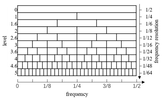
Figure 1.
1/3-binary tree filter bank.
In the entire iterative process, the number of filtering sequences doubles, and the length is reduced by half for each layer of the binary tree, while the number increases by two times, and the size is reduced by two-thirds for each of the ternary tree layers. Overall, the increase in number and decrease in length keep the data volume unchanged. The frequency band position increases in accuracy with the decomposition level’s rise, but the obtained information’s size decreases. FK selects the optimal frequency band to balance the decomposition layer and the signal length. The above method only introduces the construction of the 1/3-binary tree filter bank in FK. For studies on this index, refer to [4].
2.2. Logarithmic Envelope Spectrum and Log-Cycligram
The joint analysis of kurtosis and envelope is one of the most successful and widely used methods in the early fault diagnosis of rolling bearings. Exploring the “most impulsive” (i.e., maximum index value) frequency band for envelope analysis has been proven effective [25]. However, the two methods are based on different analytical foundations. The former is based on the impulsiveness of the signal [3], while the latter is based on second-order cyclostationarity [23]. The second-order cyclostationary (CS2) component, a typical fault feature in rotating and alternating mechanical systems, has recently received extensive attention. The squared envelope spectrum (SES) in the analytical form of a raw signal is the most commonly used index for monitoring the CS2 component [26]. According to Parseval’s theorem, the analytical identity of the SES and the corresponding filtered signal kurtosis can be derived as follows [19]:
where is the mean operator. and , respectively, represent the squared envelope and squared envelope spectrum of the time-domain signal decomposed in the j-th segment of the i-th layer of the 1/3-binary tree filter bank, and L is the signal length. This formula converts the definition of spectral kurtosis into a function of the SES, which intuitively explains why spectral kurtosis can test impulsiveness. The value of spectral kurtosis is high when the bearing characteristic frequency exists with a high amplitude. Meanwhile, as in Equation (3), the SES can also be equivalent to the autocorrelation of the discrete Fourier transform. is the convolution operator. The presence of the CS2 component leads to an increase in the amplitude of the fault frequency and harmonic, which increases the SES value.
However, recent studies revealed that even with appropriate preprocessing (e.g., pre-whitening using ARMA linear prediction models [2]), monitoring typical healthy mechanical systems using the SES may result in false positives [17]. Considering this phenomenon, the logarithmic envelope spectrum (LES) is proposed to improve the monitoring of the CS2 component [27]. LES is defined as follows:
where obtains the logarithm with base e. and , respectively, represent the logarithmic envelope and logarithmic envelope spectrum of the time-domain signal decomposed in the j-th segment of the i-th layer.
The LES can comprehensively analyze the impulsiveness and cyclostationarity of the signal. The advantage of the LES over the SES lies in its excellent statistical properties [23]. On the one hand, the LES is unbiased in the parameter estimation of the Gaussian white noise following the chi-square distribution. On the other hand, in the presence of harmonic interference, the LES is more confident than the SES regarding the mixture signal as a chi-square distribution. Therefore, the LES can eliminate the interference of irrelevant components better than the SES.
Based on the LES, log-cycligram (LC), which is sensitive to both impulsiveness and cyclostationarity, is proposed as follows [24]:
where indicates the sum of the maximum values of each in the cycle range of the i-th layer and the j-th segment when the cyclic narrowband is preset as N. Usually, the number of harmonics involved in the calculation is not expected to exceed 4 [22] because the computational complexity is affected by the number. Under the environment of strong noise and transient pulse interference, LC has been proven more accurate in frequency band extraction than FK, Infogram, Protrugram, and Autogram, which employ the SES [24].
In bearing diagnosis with random sliding of the rollers, like other methods for narrow bands, LC may increase the probability of uncorrelated disturbances affecting the detection of CS2 components if the narrow band is vast. However, research [2] shows that the slip rate does not usually exceed 2%. By computing the envelope spectrum, this probability can be further reduced. As for the number of fault frequencies, for a single fault, the fault frequencies of all the possible fault locations (e.g., outer race, inner race, and roller) can be brought into Equation (6) as the band of interest for calculation; for composite faults, separately calculating them is the best approach.
2.3. Envelope Harmonic-to-Noise Ratio
In bioacoustics, the HNR is an effective method of characterizing acoustic periodicity and hoarseness. Xu et al. recently introduced this concept into the field of bearing fault diagnosis and proposed the envelope harmonic-to-noise ratio (EHNR). Using the envelope rather than the signal itself, the EHNR can effectively identify faults [21]. The basic formula for the HNR is as follows:
where H represents the energy of the harmonic components, and N represents the energy of the noise components. Given that the ideal characteristic information of bearing faults is periodic pulses at specific intervals, the fault impulse could excite multiple resonant frequencies. In theory, the envelope signal can be viewed as the sum of harmonic and noise components. Therefore, the EHNR can be expressed as follows [21]:
where represents the autocorrelation operation. is the lag value that maximizes the autocorrelation of . represents the harmonic energy, while represents the total energy. is of the decomposed signal corresponding to the i-th layer and the j-th segment.
In fault diagnosis, the EHNR is related to correlation, which can characterize periodic pulses well, that is, the fault component, and is positively correlated with the fault energy. However, there are also two problems with EHNR. On the one hand, the autocorrelation calculation must set a short window, which is challenging to define correctly in practice [28]. On the other hand, the bearing fault signal does not strictly obey second-order cyclostationary but pseudo-cyclostationary, resulting in deviation. Thus, and are not directly equivalent to the energy of the harmonic and noise in actual nonstationary signals [29], but the concept of HNR is still an excellent reference.
3. Proposed Method
In this section, the cyclic narrowband of LC is expanded to the cyclic sub-band (BC) model. The global and local thresholds for excluding outliers are designed based on the statistical properties of the LES and the HNR, respectively. Finally, a new indicator, WGCRE, is proposed and introduced into the 1/3-binary tree filter bank to extract the optimal demodulation frequency band.
3.1. Model of Cyclic Sub-Band
To address Problems 1 and 2 in the Introduction (Section 1), the cyclic narrowband in LC is reconstructed and extended to the cyclic sub-band (BC) model for the fault and its surrounding noise. Some improvements have been made to the cyclic narrowband to achieve the local refinement of the index and highlight the amplitude of the fault frequency. As shown in Figure 2, the signal is divided into several sub-bands with unequal lengths, covering the actual bearing characteristic frequency or its harmonics in the frequency domain. In , great attention is paid to the bearing characteristic frequency in fault narrowband , while other components are ignored. Meanwhile, the noise band is refined into left and right noise narrowband groups and . The specific construction of the BC model is as follows:
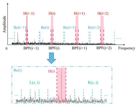
Figure 2.
Schematic of BC division.
3.1.1. The Determination of the Fault Narrowband
Theoretical bearing characteristic frequency can be calculated based on the inherent properties of the bearing and rotational speed, according to [2]. The failure frequency here refers to the single failure frequency of the inner race, the outer race, or the rolling element. The actual fault frequency and harmonics () could then be calculated:
where is the operation to find the point of maximum value in range . Meanwhile, the left and right boundaries ( and , respectively) of could be defined as follows:
where is the specific error value, satisfying , and is the relative error. Given the pseudo-cyclostationarity of the fault signal, fault frequency BPF may slip within a particular range [30], and this relative error () is generally 1–2% [16]. To ensure that is always within , the relative error () is selected as 2%. Rather than directly selecting the theoretical bearing characteristic frequency and harmonics as the calculated values, taking the maximum value in as the actual value according to Equations (9)–(11) can accurately determine the position of the next-order fault harmonic, thus defining the narrowband (). Considering that the gap between the actual harmonic and the theory will gradually increase with the accumulation of errors, the narrowband width is a linear function that varies with .
3.1.2. The Definition of the Left and Right Noise Narrowband Groups
Based on the position of , a set of left and right noise narrow bands ( and ) with ranges of and are, respectively, defined as follows:
where , while is the number of or . To ensure that the widths of and are equal to with full data utilization, the following should be satisfied:
where denotes the rounding to 0, such that ⌊3.7⌋ = 3.
3.1.3. The Acquisition of the Cyclic Sub-Band
Combining , , and , cyclic sub-band can be obtained. Each has a corresponding fault and noise part. If the ratio of the energy of the fault part to the noise is large, then this segment has a large amount of fault information. A large ratio in each indicates that this demodulated signal can reflect the fault characteristics. This ratio is the cyclic logarithmic HNR (CLHNR) mentioned next.
3.2. Cyclic Relative Entropy with Thresholds
Referring to the definition of the HNR, the CLHNR based on the LES can be obtained as follows:
In addition to a high degree of identification for and , the expected index should be sensitive enough to the large amplitude and energy of . Thus, a good index, that is, CRE, is defined as follows:
The CRE based on the cyclic sub-band is theoretically reasonable and has a certain similarity in design with the Kullback–Leibler divergence [31]. However, two defects remain. (1) Irrelevant frequency may be selected as in the absence of fault in . (2) In the presence of a fault in , CRE may be abnormally large when harmonic interference exists or negative when is more minor than . Therefore, the CRE must be limited by some thresholds.
For Defect 1, two assumptions are first set:
- Assumption 1: belongs to the white noise component.
- Assumption 2: does not belong to the white noise component.
The SES and LES of complex white noise separately obey the following chi-square distribution with 2 degrees of freedom [23]:
The LES of complex white noise has a unique property. The scale factor is known in advance and does not depend on the characteristics of the signal other than length N. Thus, in the process of judging white noise, the LES is superior to the SES. According to Equation (18), the global threshold parameter η can be obtained as follows:
where p is the probability of a false alarm and is set to 0.01 in this paper. A 99% confidence level in probability and statistics is sufficient to determine whether the event is valid. The amplitudes of the LES could be re-defined as follows:
To avoid the influence of the absence of fault and extreme outliers, upper and lower thresholds are set for the LES, and linear scaling is performed. If Assumption 1 is satisfied and 0.1 is taken as the amplitude. If , Assumption 2 is met.
For Defect 2, considering the existence of harmonic interference, an upper threshold is set for . When the upper threshold is reached, a great degree of discrimination exists. To avoid a negative CRE, a local threshold is established for the CLHNR part. When CLHNR < , let CLHNR = . is a tiny value set to 0.001 in this paper. is set to 0.001 to ensure the parameter is small enough to affect the subsequent calculation and not set to 0 to ensure the analysis does not ignore the influence of other sub-bands in the following geometric weighting.
After setting the global and local thresholds, the CRE can screen potential fault characteristic frequencies during calculation, reducing the error in selecting the possibility of white noise or harmonic interference. A large CRE in particular means that the corresponding frequency is likely the fault frequency or its harmonics. In addition, if the CRE in two continuous is not prominent, the following higher harmonics calculation will be terminated. This approach can identify the fault well, avoid noise masking, and save computing time.
3.3. Weighted Geometric Cyclic Relative Entropy
By synthetically substituting the CRE in each into the geometric mean calculation, the GCRE could be obtained as follows:
where N represents the number of selected . The higher N means a more straightforward diagnosis and a higher calculation cost. N is set to 5 in this paper.
The main failures of bearings are inner race, outer race, and rolling element failures [2]. Thus, the GCRE corresponding to the three fault conditions is obtained, and the corresponding average MGCRE is calculated as follows:
Then, the benchmark value of BGCRE is defined as follows:
where σ represents the scale factor . In most cases, the scale factor is taken to be 1. The “mean principle” [32] ensures that the GCRE participating in the weighting under different fault types satisfies the presence of the corresponding fault. If , it has no corresponding fault type on the demodulation frequency band and does not participate in the weighting calculation. Then, is defined after screening by the BGCRE, and the final index (WGCRE) is obtained as follows:
After defining the WGCRE, the optimal frequency band could be obtained, as shown in Figure 3. The main steps are 3 and 4, where the BC model is established and WGCRE with thresholds is defined.
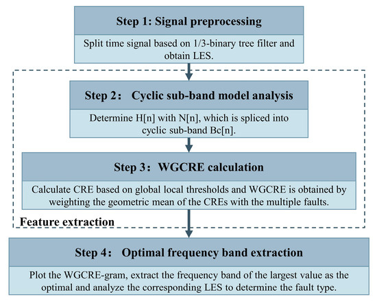
Figure 3.
Approach steps.
4. Comparison of Numerically Generated Signals
A vibration signal model of a single-fault bearing under the influence of different exogenous noises is constructed in this section.
4.1. Rolling Bearing Vibration Signal Composition
The rolling bearing vibration signal spectrum comprises the fundamental and harmonics vibration component, the impulse vibration component, and the noise component.
4.1.1. Fundamental and Harmonics Vibration Component
Under normal working conditions, the fundamental vibration component is mainly a cosine signal whose frequency is the rotational frequency. Given the vibration caused by shaft bending, cracks, installation errors, and so on, the harmonic frequency must be considered. Therefore, the fundamental and harmonics vibration component can be represented as follows:
where are the fundamental frequency and harmonics. , , and are the order, amplitude, and phase of the basic and harmonic vibration components, respectively.
4.1.2. Impulse Vibration Component
When local damage, such as pitting, spalling, and other faults, occurs during the operation, a periodic impulse is generated, stimulating the damped natural vibration. Therefore, the vibration signal usually contains the following impulse vibration component:
where represents the periodic impulse, and is the amplitude. , , and are the damping ratio, the natural frequency of the bearing system, and the damping attenuation frequency (), respectively. is the period, that is, the reciprocal of the bearing characteristic frequency.
4.1.3. Noise Component
As long as the bearing is running, it will generate noise. Noise is caused by many factors, including the impact of the rolling elements and environmental noise, which have strong randomness.
4.2. Single-Fault Vibration Model
Based on the signal composition, the single-fault vibration model can be obtained as follows:
The first term is the rotation frequency with two harmonics, the second is the bearing characteristic frequency with four harmonics, the third is the fault impulse vibration, the fourth is the exogenous noise, and the last is Gaussian white noise. is a typical random sequence with a mean of 1 and a standard deviation of 0.1, while is a convolution operator. The relevant parameters are set as shown in Table 1, where is the sampling frequency.

Table 1.
The parameters in the single-fault vibration model.
For exogenous noise with different HNRs set by scale factor B and five types of noises, as shown in Figure 4, are added to the model:
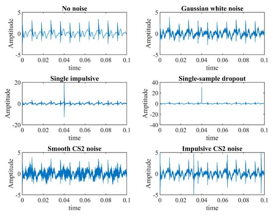
Figure 4.
Different exogenous noises.
- Single impulse:where and ;
- Single-sample dropout: A one-sample outlier with an amplitude of 30 at 0.04 s;
- Smooth CS2 noise:where and ;
- Impulsive CS2 noise:where and .
4.3. Comparison under Different Exogenous Noise
Based on the single-fault vibration model under different exogenous noises, FK, LC, and WGCRE are compared at the optimal demodulation frequency band extraction. The HNR is adjusted by scale factor B, decreasing from 20 dB to −60 dB at the rate of 1 dB. A small HNR indicates blatant noise interference. Referring to [24], the frequency bands selected under all noise levels are drawn in a graph, clearly presenting the influence of noise. The selected frequency band does not necessarily reflect the quality of diagnosis and identification, but it can provide basic and targeted judgments.
The diagrams of the Gaussian white noise, the single impulse, the single-sample dropout, the smooth CS2 noise, and the impulsive CS2 noise are presented in Figure 5, Figure 6, Figure 7, Figure 8 and Figure 9. The black and red dotted lines represent the fault and noise resonance frequency, respectively. The demodulation frequency band covering or near the black dotted line has a good diagnostic effect, while that near the red line is susceptible to the corresponding noise. Moreover, the narrower the selected band is, the more accurate the demodulation performance will be.
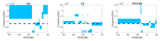
Figure 5.
Selected optimal demodulation bands under Gaussian white noise for different HNR.
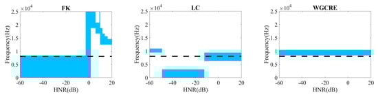
Figure 6.
Selected optimal demodulation bands under single impulse for different HNR.
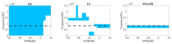
Figure 7.
Selected optimal demodulation bands under single-sample dropout for different HNR.
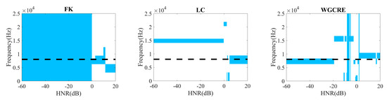
Figure 8.
Selected optimal demodulation bands under smooth CS2 noise for different HNR.
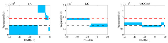
Figure 9.
Selected optimal demodulation bands under impulsive CS2 noise for different HNR.
It is worth noting that when the HNR is small, the kurtosis of FK, the narrow band amplitude of LC, and the relative entropy of WGCRE will be disturbed by different levels due to the fault signal drowning in the noise. Therefore, to a certain extent, if it can still perform well in an intense noise environment, it can prove that WGCRE has good robustness to external noise.
In Figure 5, under Gaussian white noise, FK can only select the frequency band containing the fault resonance frequency near 0 dB. However, LC and WGCRE can choose the band covering or near the fault resonance frequency in most cases, where the bandwidth is much narrower. Overall, the WGCRE can often select a reasonable frequency band. It is worth mentioning that when the HNR is close to −20 dB, FK, LC, and WGCRE all produce large fluctuations. It takes more than −20 dB to stabilize, but the center frequency is offset from the theoretical fault resonance frequency. The offset here may be due to the white noise intensity increasing to a critical point, and the signal is gradually drowned out by noise, resulting in distortion in the selected frequency band. As the white noise rises further, the signal is completely drowned out, and the center frequency of the optimal band is naturally set to stabilize. Still, a specific offset is generated due to the white noise as the dominance. FK is the kurtosis of the calculation, and while white noise drowns out the prominent signal, the deviation will naturally be significant. LC and WGCRE consider the amplitude of the corresponding fault frequency and the relative noise size of the amplitude after frequency band envelope demodulation, which naturally has less impact.
In Figure 6, FK has noticeable distortion under a single impulse where the HNR is greater than 0 dB. The bandwidth is too enormous to demodulate where the HNR is less than 0 dB. LC exhibits an excellent demodulation performance where the HNR is greater than −10 dB. Still, the diagnosis has a noticeable distortion in the intense noise environment where the HNR is less than −10 dB. The demodulation band of WGCRE fails to cover but is near the fault resonance frequency and has a much smaller demodulation bandwidth than the other two. Therefore, the fault signal in WGCRE can still be globally diagnosed.
In Figure 7, under single-sample dropout, FK fails to detect the optimal demodulation band where the HNR is greater than 5 dB, and the bandwidth is vast where the HNR is less than 5 dB. LC has a good demodulation performance where the HNR is greater than −10 dB but not ideal where the HNR is less than −10 dB. WGCRE can globally select a very outstanding demodulation frequency band, and the accuracy is extremely high.
In Figure 8, under smooth CS2 noise, FK has noticeable distortion where the HNR is greater than 10 dB, the bandwidth is enormous, and the accuracy is insufficient where the HNR is less than 0 dB. LC has a good demodulation performance when the HNR is greater than 5 dB, a poor performance in the intense noise environment where the HNR is less than 5 dB. WGCRE can select an ideal demodulation band in −20 dB to 0 dB, covering or near the fault resonance frequency, and the bandwidth is small, with higher accuracy than the former two. The smooth CS2 noise intensity continues to increase, and the FK and LC are distorted at the optimal frequency band selected at low HNR. While WGCRE overcomes this flaw in most cases, there are still miscalculations when the HNR approaches −20 dB. The reason may be that the smooth CS2 noise is similar to the fault signal at this time because they are all cyclostationary, which causes the misjudgment of the noise as a fault signal. In turn, this causes the natural fault frequency to be higher than the actual. After its energy gradually increases, the characteristics of smooth CS2 noise become more apparent, and WGCRE can distinguish it based on relative entropy. However, LC is based on the magnitude and still considers it part of the fault and, therefore, cannot reject it.
In Figure 9, under impulsive CS2 noise, FK has low accuracy where the HNR is greater than −10 dB and the selected frequency band is near the noise resonance frequency band. This noise has a substantial interference, the same as LC, where the HNR is less than −20 dB. Moreover, the bandwidth in FK is vast when the HNR is less than 0 dB. However, WGCRE has perfect global performance and accuracy.
The comparison of the three different methods under five exogenous noises reveals the following:
- For the model that only adds Gaussian white noise, FK is easily affected by intense noise, whereas LC and WGCRE have good robustness globally.
- When adding single impulse or single-sample dropout, FK still has certain disadvantages; LC performs well, but considerable fluctuations remain in intense noise environments; WGCRE shows strong robustness and is unaffected.
- When smooth CS2 noise is added, FK can select the correct frequency band, but most of the bandwidth is extremely large with low accuracy. LC is wholly distorted in a robust noise environment. WGCRE also has distortion but still has a good advantage where the HNR is enormous, covering the fault resonance frequency and presenting high accuracy.
- For impulsive CS2 noise, FK has distortion in the weak noise environment; LC is distorted in the intense noise environment; only WGCRE maintains good frequency band extraction performance globally.
In general, for this single faulty rolling bearing model with different exogenous noises added, the performance of WGCRE is excellent. However, specific situations must be experimentally verified.
5. Comparison on Experimentally Measurement
5.1. Introduction to Experimental Data
To verify the correctness and rationality of the proposed method (i.e., WGCRE), multiple data were used to analyze the pros and cons of the three extraction methods: FK, LC, and WGCRE. Higher numbers and larger amplitudes of the BPFs with harmonics captured in the LES and the more negligible noise imply more accurate and rational diagnosis results.
The fault types of the bearing in the data include the outer race, inner race, and compound inner and outer race faults (see Figure 10 for the types of rolling bearing faults). The experimental signals used are from the bearing data Center of Case Western Reserve University (CWRU), the condition monitoring experimental dataset based on vibration and motor current signals of Paderborn University (UPB), and the data of the HZXT-008 bearing experimental platform (HZXT-008). Moreover, all data were pre-whitened according to [2] to remove linearly predictable components before analysis.
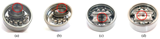
Figure 10.
The common fault of rolling bearing: (a) outer race crack; (b) outer race pitting; (c) inner race crack; (d) inner race pitting.
Six experimental data sets were analyzed, including two outer race faults, two inner race faults, and two compound faults. The experimental data are all from the drive end. According to [2], the corresponding inner and outer race characteristic frequencies (BPFI, BPFO) can be calculated. Other important parameters, such as the sampling frequency (Fs) and the rotation speed (w), are shown in Table 2.
Table 2.
Experimental data statistics.
CWRU experiments [33] collected the drive-end vibration signals through an acceleration sensor. The experimental bearings are SKF 6205. The bearing faults were captured by electrical discharge machining (EDM) single-point damage, and the inner and outer fault types were cracks. Both damage diameters were 0.007 inches.
The UPB experiments [34] mainly consist of a bearing housing and an electric motor. The experimental bearing is MTK 6203. The radial load applied to the practical approach was more significant than the bearing load under normal conditions, shortening the bearing life and accelerating the fatigue damage. The inner and outer fault types were single-point pitting caused by accelerated lifetime tests through overload, wrong viscosity, and contamination. The damage geometry was 1.5 mm long and 6 mm wide.
The HZXT-008 bearing experimental platform is shown in Figure 11. It comprises a control device, a DC drive motor, a reducer, drive and fan end bearings, two acceleration sensors, and a fan. The control device adjusts the speed, and the DC drive motor drives the entire platform through the coupling. The acceleration sensor is mounted on the bearing housing of the drive fan end. The experimental bearing is NSK 6200. Four bearing failure types were simulated by EDM, as shown in Figure 10. The inner and outer fault types in Case 2 and Case 6 were 1.2 mm deep cracks, and the inner fault in Case 4 was single-point pitting with a 1.2 mm damage diameter.
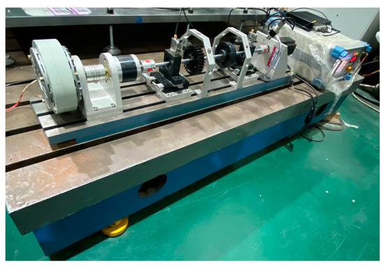
Figure 11.
HZXT-008 bearing experimental platform.
5.2. Single-Fault Diagnosis
5.2.1. Outer Race Fault Diagnosis
The outer race fault data adopt the CWRU experiment (Case 1) and is verified with the HZXT-008 (Case 2). The numbers of captured BPFOs, which could reflect the fault location, are listed in Table 3.
Table 3.
Captured serial numbers n of BPFs with computation cost t statistics table.
For Case 1, we used a low sampling frequency for analysis, and the extraction of optimal demodulation frequency bands and the corresponding LES of FK, LC, and WGCRE are shown in Figure 12. FK, LC, and WGCRE elite the bands at Level 3 with a center frequency of 5625 Hz, Level 4 with 5437.5 Hz, and Level 2.6 with 1500 Hz as the optimal bands, respectively. Given the low sampling frequency and the high-level selection, the LES of FK and LC is extremely short of analyzing the high harmonics. However, they could be accurately detected in WGCRE. WGCRE could capture more BPFO with harmonics than the other two, and their computation costs are approximately equal.
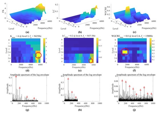
Figure 12.
Optimal bands extraction of Case 1 (outer race fault). (a–f) are 3D and 2D FK, LC, and WGCRE–gram, respectively (optimal bands are circled in red). (g,h,j) are LES of FK, LC, and WGCRE, respectively (BPFOs with harmonics are marked with red triangles).
At the low sampling frequency, less and less information can be obtained as the number of decomposition layers increases. Therefore, the decomposition frequency band that is too high is not conducive to fault diagnosis. FK and LC have entered the misunderstanding of blindly pursuing the overall kurtosis and high amplitude, so the high-level frequency band with less information is identified as optimal, leading to their inability to analyze too many fault frequency multiplications. Due to the geometric average in WGCRE, the overall large can only be satisfied when the amplitude of each octave is large. This operation ensures that the extracted optimal frequency band contains more fault multiplication information in WGCRE.
For Case 2, FK, LC, and WGCRE extract the bands at Level 2.6 with a center frequency of 22,000 Hz, Level 4 with 20,250 Hz, and Level 3.6 with 15,000 Hz, respectively, in Figure 13. WGCRE can capture six BPFOs, thus better than FK and LC. Moreover, in the LES of the WGCRE, the fault information is prominent with a small amplitude of the noise component. As for the computation costs, WGCRE could catch up with LC to a certain extent.
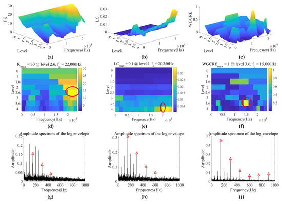
Figure 13.
Optimal bands extraction of Case 2 (outer race fault). (a–f) are 3D and 2D FK, LC, and WGCRE–gram, respectively (optimal bands are circled in red). (g,h,j) are LES of FK, LC, and WGCRE, respectively (BPFOs with harmonics are marked with red triangles).
FK only focuses on the kurtosis of a given signal but does not consider whether the main contributor is faulty. In this case, unrelated impact noise is the most significant contributor. The diagnostic capabilities of FK are weakened due to interference from impact noise, and LC performs better in this regard. WGCRE goes further, selecting a band with a smaller noise amplitude by setting local thresholds in Section 3, and the entire spectrum is extremely clean.
5.2.2. Inner Race Fault Diagnosis
The inner race fault data also adopt the CWRU (Case 3) and HZXT-008 (Case 4) experiments, and the numbers of captured BPFIs are listed in Table 3.
For Case 3, FK, LC, and WGCRE select the bands at Level 4 with a center frequency of 11,250 Hz, Level 4 with 2250 Hz, and Level 3 with 13,500 Hz as the optimal bands, respectively, in Figure 14. WGCRE can capture six BPFIs more than FK and LC. FK only captures two BPFIs under this data which LES has an intense noise; consequently, it is difficult to clarify whether they are from harmonic interference or fault signal.
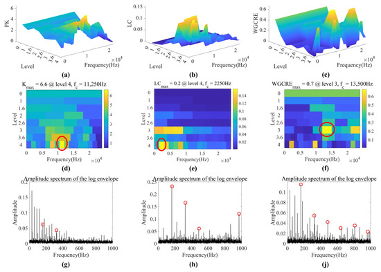
Figure 14.
Optimal bands extraction of Case 3 (inner race fault). (a–f) are 3D and 2D FK, LC, and WGCRE–gram, respectively (optimal bands are circled in red). (g,h,j) are LES of FK, LC, and WGCRE, respectively (BPFIs with harmonics are marked with red circles).
In the face of this inner ring, the diagnosis of FK is even more disturbed by noise than in Case 2, so it is impossible to determine whether the fault exists. LC and WGCRE are also subject to noise interference but can achieve basic diagnostics. However, due to the lack of fourth and fifth harmonics information in the extraction frequency band, LC can still misjudge the diagnosed fault as harmonic interference. WGCRE, on the other hand, circumvents these confusions by setting local thresholds in Section 3.
For Case 4, FK, LC, and WGCRE elite the bands at Level 1 with a center frequency of 18,000 Hz, Level 4 with 750 Hz, and Level 3.6 with 3000 Hz, respectively, in Figure 15. In the LES of WGCRE, the amplitude of the noise component is small, and the fault information is prominent.
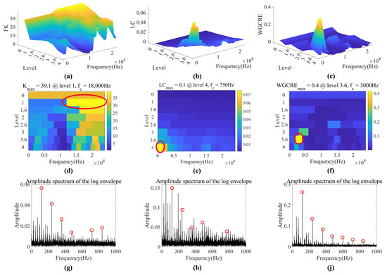
Figure 15.
Optimal bands extraction of Case 4 (inner race fault). (a–f) are 3D and 2D FK, LC, and WGCRE–gram, respectively (optimal bands are circled in red). (g,h,j) are LES of FK, LC, and WGCRE, respectively (BPFIs with harmonics are marked with red circles).
This case fully demonstrates the advantages of WGCRE in setting global and local thresholds. The global threshold ensures a small noise amplitude, and the local provides sufficiently prominent fault information. Because of these two thresholds, WGCRE can stand out in this case without having to extricate itself from the quagmire of intense noise like FK and LC.
5.3. Compound Fault Diagnosis
The compound fault data adopts UPB (Case 5) and HZXT-008 (Case 6). The numbers of captured BPFOs and BPFIs are listed in Table 3.
The captured BPFOs and BPFIs of Case 5 are marked with red triangles and circles, respectively, in Figure 16. FK, LC, and WGCRE elite the bands at Level 1 with a center frequency of 24,000 Hz, Level 3.6 with 30,666.66 Hz, and Level 2.6 with 13,333.33 Hz, respectively. WGCRE can capture nine BPFOs and seven BPFIs, thus better than FK and LC.
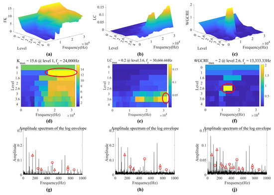
Figure 16.
Optimal bands extraction of Case 5 (compound fault). (a–f) are 3D and 2D FK, LC, and WGCRE–gram, respectively (optimal bands are circled in red). (g,h,j) are LES of FK, LC, and WGCRE, respectively (BPFOs with harmonics are marked with red triangles and BPFIs are with red circles).
In the face of compound fault, the situation is more complicated, and noise is inevitable to a certain extent. The optimal bands of FK and LC can no longer recognize nearly half of the fault harmonics. However, WGCRE still chooses the bar containing the most prominent harmonics as much as possible and can still make certain judgments.
As for Case 6, the optimal band extraction and the corresponding LES are shown in Figure 17. FK, LC, and WGCRE select the bands at Level 4 with a center frequency of 21,750 Hz, Level 4 with 2250 Hz, and Level 2 with 15,000 Hz, respectively. The noise amplitude in FK is enormous, which influences judgment. LC only captures two BPFOs and two BPFIs; too challenging to determine these two faults’ positions. WGCRE can capture eight BPFOs and eight BPFIs, thus better than FK and LC.
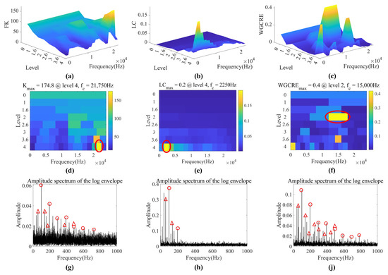
Figure 17.
Optimal bands extraction of Case 6 (compound fault). (a–f) are 3D and 2D FK, LC, and WGCRE–gram, respectively (optimal bands are circled in red). (g,h,j) are LES of FK, LC, and WGCRE, respectively (BPFOs with harmonics are marked with red triangles and BPFIs are with red circles).
In this case, WGCRE’s performance is even more prominent. FK suffered from substantial white noise interference, and the fault information was drowned out by noise. LC shows only two fault multipliers and cannot determine whether it is fault information or harmonic interference. Only WGCRE overcomes intense white noise and harmonic interference due to the analysis of GCRE in Section 3 and the index weighting of each composite fault.
Overall, although having a blemish in computation cost, WGCRE has a significant advantage in fault diagnosis precision over the other two. The proposed method can automatically optimize the compound faults analysis to guide the band extraction, which is a significant contribution.
6. Conclusions
This paper proposes a new index, WGCRE, to extract the optimal demodulation band. This method has stronger robustness than FK and LC under external noise interference and a significant advantage in diagnosing single and compound faults of rolling bearings. Considering the pseudo-cyclostationarity of the fault, the signal is divided using the BC model, and CRE is defined in each sub-band. To exclude the influence of outliers, global and local thresholds are established. For compound faults, the WGCRE is determined by geometrically averaging and weighting the CRE of each sub-band. Moreover, the LES, which is superior to the SES, is used to demodulate the signal. The signal simulations under five different noises show that WGCRE has stronger robustness than FK and LC. Meanwhile, six rolling bearing fault experiments proved that WGCRE could more accurately and effectively diagnose the single outer or inner ring fault and compound fault of rolling bearings. The simulation and experiment results analysis finally proved that the proposed method has a better effect on compound fault diagnosis and stronger robustness than FK and LC.
It is worth noting that WGCRE is a little inferior to FK and LC in terms of computation cost due to the more complex indicators. It needs improvement later. In addition, the noise interference at about −20 dB HNR during simulation still cannot be overcome, and further progress is required. On the whole, however, WGCRE still has considerable prospects for excavation, which is worth further studying.
Author Contributions
Conceptualization, C.W. and J.X.; methodology, C.W.; software, C.W.; validation, C.W. and A.G.; formal analysis, C.W. and A.G.; investigation, C.W. and A.G.; resources, C.W.; data curation, C.W.; writing—original draft preparation, C.W.; writing—review and editing, C.W. and A.G.; visualization, C.W.; supervision, C.W.; project administration, C.W.; funding acquisition, J.X. All authors have read and agreed to the published version of the manuscript.
Funding
This research was funded by the National Key R&D Program of China (Grant No. 2020YFB2007700), and the National Natural Science Foundation of China (Grant No. 52175094).
Institutional Review Board Statement
Not applicable.
Informed Consent Statement
Not applicable.
Data Availability Statement
Not applicable.
Conflicts of Interest
The authors declare no conflict of interest.
References
- Tandon, N.; Choudhury, A. A review of vibration and acoustic measurement methods for the detection of defects in rolling element bearings. Tribol. Int. 1999, 32, 469–480. [Google Scholar] [CrossRef]
- Randall, R.B.; Antoni, J. Rolling element bearing diagnostics—A tutorial. Mech. Syst. Signal Process. 2011, 25, 485–520. [Google Scholar] [CrossRef]
- Antoni, J. The spectral kurtosis: A useful tool for characterising nonstationary signals. Mech. Syst. Signal Process. 2006, 20, 282–307. [Google Scholar] [CrossRef]
- Antoni, J. Fast computation of the kurtogram for the detection of transient faults. Mech. Syst. Signal Process. 2007, 21, 108–124. [Google Scholar] [CrossRef]
- Antoni, J. The infogram: Entropic evidence of the signature of repetitive transients. Mech. Syst. Signal Process. 2016, 74, 73–94. [Google Scholar] [CrossRef]
- McDonald, G.L.; Zhao, Q.; Zuo, M.J. Maximum correlated Kurtosis deconvolution and application on gear tooth chip fault detection. Mech. Syst. Signal Process. 2012, 33, 237–255. [Google Scholar] [CrossRef]
- Yu, X.; Huangfu, Y.; He, Q.; Yang, Y.; Du, M.; Peng, Z. Gearbox fault diagnosis under nonstationary condition using nonlinear chirp components extracted from bearing force. Mech. Syst. Signal Process. 2021, 180, 109440. [Google Scholar] [CrossRef]
- Su, H.; Shi, T.; Chen, F.; Huang, S. New method of fault diagnosis of rotating machinery based on distance of information entropy. Front. Mech. Eng. 2011, 6, 249–253. [Google Scholar] [CrossRef]
- Kong, Y.; Wang, T.; Li, Z.; Chu, F. Fault feature extraction of planet gear in wind turbine gearbox based on spectral kurtosis and time wavelet energy spectrum. Front. Mech. Eng. 2017, 12, 406–419. [Google Scholar] [CrossRef]
- Zhang, H.; Chen, X.; Du, Z.; Yan, R. Kurtosis based weighted sparse model with convex optimization technique for bearing fault diagnosis. Mech. Syst. Signal Process. 2016, 80, 349–376. [Google Scholar] [CrossRef]
- Wang, L.; Liu, Z.; Cao, H.; Zhang, X. Subband averaging kurtogram with dual-tree complex wavelet packet transform for rotating machinery fault diagnosis. Mech. Syst. Signal Process. 2020, 142, 106755. [Google Scholar] [CrossRef]
- Wang, D.; Zhao, Y.; Yi, C.; Tsui, K.-L.; Lin, J. Sparsity guided empirical wavelet transform for fault diagnosis of rolling element bearings. Mech. Syst. Signal Process. 2018, 101, 292–308. [Google Scholar] [CrossRef]
- Miao, Y.; Wang, J.; Zhang, B.; Li, H. Practical framework of Gini index in the application of machinery fault feature extraction. Mech. Syst. Signal Process. 2021, 165, 108333. [Google Scholar] [CrossRef]
- Wang, D.; Miao, Q. Smoothness index-guided Bayesian inference for determining joint posterior probability distributions of anti-symmetric real Laplace wavelet parameters for identification of different bearing faults. J. Sound Vib. 2015, 345, 250–266. [Google Scholar] [CrossRef]
- Hou, B.; Wang, D.; Xia, T.; Wang, Y.; Zhao, Y.; Tsui, K.-L. Investigations on quasi-arithmetic means for machine condition monitoring. Mech. Syst. Signal Process. 2021, 151, 107–451. [Google Scholar] [CrossRef]
- Antoni, J.; Randall, R. Differential Diagnosis of Gear and Bearing Faults. J. Vib. Acoust. Trans. ASME. 2002, 124, 165–171. [Google Scholar] [CrossRef]
- Borghesani, P.; Antoni, J. CS2 analysis in presence of non-Gaussian background noise–Effect on traditional estimators and resilience of log-envelope indicators. Mech. Syst. Signal Process. 2017, 90, 378–398. [Google Scholar] [CrossRef]
- Barszcz, T.; JabŁoński, A. A novel method for the optimal band selection for vibration signal demodulation and comparison with the Kurtogram. Mech. Syst. Signal Process. 2011, 25, 431–451. [Google Scholar] [CrossRef]
- Borghesani, P.; Pennacchi, P.; Chatterton, S. The relationship between kurtosis- and envelope-based indexes for the diagnostic of rolling element bearings. Mech. Syst. Signal Process. 2014, 43, 25–43. [Google Scholar] [CrossRef]
- Moshrefzadeh, A.; Fasana, A. The Autogram: An effective approach for selecting the optimal demodulation band in rolling element bearings diagnosis. Mech. Syst. Signal Process. 2018, 105, 294–318. [Google Scholar] [CrossRef]
- Xu, X.; Zhao, M.; Lin, J.; Lei, Y. Envelope harmonic-to-noise ratio for periodic impulses detection and its application to bearing diagnosis. Meas. J. Int. Meas. Confed. 2016, 91, 385–397. [Google Scholar] [CrossRef]
- Mo, Z.; Wang, J.; Zhang, H.; Miao, Q. Weighted Cyclic Harmonic-to-Noise Ratio for Rolling Element Bearing Fault Diagnosis. IEEE Trans. Instrum. Meas. 2020, 69, 432–442. [Google Scholar] [CrossRef]
- Borghesani, P.; Shahriar, M.R. Cyclostationary analysis with logarithmic variance stabilisation. Mech. Syst. Signal Process. 2016, 70–71, 51–72. [Google Scholar] [CrossRef]
- Smith, W.A.; Borghesani, P.; Ni, Q.; Wang, K.; Peng, Z. Optimal demodulation-band selection for envelope-based diagnostics: A comparative study of traditional and novel tools. Mech. Syst. Signal Process. 2019, 134, 106303. [Google Scholar] [CrossRef]
- Zhang, Y.; Randall, R. Rolling element bearing fault diagnosis based on the combination of genetic algorithms and fast kurtogram. Mech. Syst. Signal Process. 2009, 23, 1509–1517. [Google Scholar] [CrossRef]
- He, X.; Liu, Q.; Yu, W.; Mechefske, C.K.; Zhou, X. A new autocorrelation-based strategy for multiple fault feature extraction from gearbox vibration signals. Measurement 2021, 171, 108738. [Google Scholar] [CrossRef]
- Antoni, J.; Borghesani, P. A statistical methodology for the design of condition indicators. Mech. Syst. Signal Process. 2019, 114, 290–327. [Google Scholar] [CrossRef]
- Xu, X.; Zhao, M.; Lin, J.; Lei, Y. Periodicity-based kurtogram for random impulse resistance. Meas. Sci. Technol. 2015, 26, 085011. [Google Scholar] [CrossRef]
- Wang, M.; Mo, Z.; Fu, H.; Yu, H.; Miao, Q. Harmonic L2/L1 Norm for Bearing Fault Diagnosis. IEEE Access 2019, 7, 27313–27321. [Google Scholar] [CrossRef]
- Gao, S.; Han, Q.; Zhou, N.; Pennacchi, P.; Chatterton, S.; Qing, T.; Zhang, J.; Chu, F. Experimental and theoretical approaches for determining cage motion dynamic characteristics of angular contact ball bearings considering whirling and overall skidding behaviors. Mech. Syst. Signal Process. 2022, 168, 108704. [Google Scholar] [CrossRef]
- Matychyn, I. On Computation of Matrix Mittag-Leffler Function. arXiv 2017, arXiv:1706.01538. [Google Scholar]
- Wu, K.; Chu, N.; Wu, D.; Antoni, J. The Enkurgram: A characteristic frequency extraction method for fluid machinery based on multi-band demodulation strategy. Mech. Syst. Signal Process. 2021, 155, 107564. [Google Scholar] [CrossRef]
- Smith, W.A.; Randall, R.B. Rolling element bearing diagnostics using the Case Western Reserve University data: A benchmark study. Mech. Syst. Signal Process. 2015, 64–65, 100–131. [Google Scholar] [CrossRef]
- Kimotho, J.K.; Lessmeier, C.; Sextro, W.; Zimmer, D. Condition monitoring of bearing damage in electromechanical drive systems by using motor current signals of electric motors: A benchmark data set for data-driven classification. Third Eur. Conf. Progn. Health Manag. Soc. 2016, 3, 152–156. [Google Scholar]
Disclaimer/Publisher’s Note: The statements, opinions and data contained in all publications are solely those of the individual author(s) and contributor(s) and not of MDPI and/or the editor(s). MDPI and/or the editor(s) disclaim responsibility for any injury to people or property resulting from any ideas, methods, instructions or products referred to in the content. |
© 2022 by the authors. Licensee MDPI, Basel, Switzerland. This article is an open access article distributed under the terms and conditions of the Creative Commons Attribution (CC BY) license (https://creativecommons.org/licenses/by/4.0/).