Unsupervised Tool Wear Monitoring in the Corner Milling of a Titanium Alloy Based on a Cutting Condition-Independent Method

Abstract

Real-time tool condition monitoring (TCM) for corner milling often poses significant challenges. On one hand, corner milling requires configuring complex milling paths, leading to the failure of conventional feature extraction methods to characterize tool conditions. On the other hand, it is costly to obtain sufficient test data on corner milling for most of the current pattern recognition methods, which are based on the supervised method. In this work, we propose a time-frequency intrinsic feature extraction strategy of acoustic emission signal (AEs) to construct a cutting condition-independent method for tool wear monitoring. The proposed new feature-extraction strategy is used to obtain the tool wear conditions through the intrinsic information of the time-frequency image of AEs. In addition, an unsupervised tool condition recognition framework, including the unsupervised feature selection, the clustering based on adjacent grids searching (CAGS) and the density factor based on CAGS, is proposed to determine the relationship between tool wear values and AE features. To test the effectiveness of the monitoring system, the experiment is conducted through the corner milling of a titanium alloy workpiece. Five metrics, PUR, CSM, NMI, CluCE and ClaCE, are used to evaluate the effectiveness of the recognition results. Compared with the state-of-the-art supervised methods, our method provides commensurate monitoring effectiveness but requires much fewer test data to build the model, which greatly reduces the operating cost of the TCM system.

1. Introduction

The important position of the tool in the cutting process has caused extensive research on the monitoring of tool wear states in the metal-cutting process [1,2], which has a history of several decades. Among them, the complex profile of aeronautical structural parts makes the sensor signal in the processing process very non-stationary, which greatly increases the monitoring difficulty. Therefore, the monitoring system is required to have higher adaptability and robustness. As an important part of signal feature extraction, its main goal is to transform the sensor signal to achieve the dimensionality reduction and de-redundancy of the original data, and extracting from it has high sensitivity, robustness and reliability for monitoring targets, so as to improve the efficiency and accuracy of pattern recognition. According to the difference of transform domain, it can be divided into feature-extraction methods based on time domain [3,4], frequency domain [4,5] and time-frequency domain [4,6,7].

In the time domain, the most commonly used features are root mean square, mean, kurtosis, standard deviation, skewness, and crest factor. Yuan et al. [8] extracted four statistical features with tool wear sensitivity in the time domain: the mean to reflect the central tendency of the signal; the root mean square (RMS) to represent the average energy of the signal in a given time interval; kurtosis (Kur) to represent signal transients and stationarity; and margin (Mar) to represent the ratio of the square root amplitude to the peak value of the signal. While these features are easy to extract and use, important information about the frequency content of the milled signal cannot be obtained and is susceptible to environmental noise. At this time, there is great advantage in performing feature extraction on the signal in the frequency domain. In the frequency domain, Fourier transform technology has been widely used for tool wear monitoring, and most of the information about the frequency components of the signal is obtained through fast Fourier transform (FFT) [9]. Niu et al. [10] presented fast Fourier transform (FFT) for frequency domain feature extraction. The features extracted from the frequency domain include peak amplitude spectrum (PAS) and peak power spectrum (PPS). During the entire milling process of cutting teeth from cutting in to cutting out, the change of signal energy can be seen from the time domain waveform of the signal, and the frequency component of the signal can be seen from the amplitude spectrum. The changes in the time domain and frequency domain can be observed in the time–frequency diagram of the signal at the same time. From the time–frequency diagram, it can be found that the frequency components of the signal have been changing with time. This time–frequency non-stationary characteristic cannot be represented by frequency domain features, so the method of time–frequency analysis can better reflect the characteristics of the signal.

There are two main ideas for extracting the time–frequency features of a signal. One is to use multi-resolution analysis methods such as wavelet decomposition [11,12], empirical mode decomposition [13] and variable mode decomposition [14,15] to decompose the signal into components in different frequency bands and then select the components for monitoring. One or more components that are sensitive to the target are reconstructed, and then the time domain and frequency domain features are extracted respectively. Gao et al. [14] used time–frequency domain methods such as variable-mode decomposition energy entropy, multi-scale power spectrum entropy, and multi-scale displacement entropy to process the processed signals collected by multiple sensors to obtain relevant feature data sets. Hao et al. [15] proposed a method for identifying the wear state of milling cutters based on optimized variational modal decomposition (VMD). Another idea is time–frequency decomposition methods such as short-time Fourier transform and wavelet transform to directly decompose the signal into a two-dimensional time–frequency plane, obtain the time–frequency diagram of the signal, and then extract the features reflecting the time–frequency characteristics of the signal from the time–frequency diagram. Zhang et al. [16] proposed a method based on time–frequency image feature extraction. The time–frequency image of the signal was obtained by wavelet transform, and then the non-subsampling contourlet transform was combined with the local binary mode (LBP) frequency image-related features.

In terms of signal preprocessing and feature extraction based on milling signals, the time-domain and frequency-domain feature-extraction methods are obviously not suitable for signal analysis with highly non-stationary characteristics in the cutting of aeronautical structural parts, and the existing time–frequency feature extraction methods mainly focusing on the frequency band energy features based on signal decomposition or the time–frequency diagram, the sensitive features in the time–frequency diagram cannot be effectively extracted, and the time–frequency diagram cannot reflect the time-varying characteristics of the instantaneous frequency components of the signal due to the influence of cutting energy. Therefore, the mining of information in the signal is not comprehensive.

On the other hand, the online monitoring of milling is essentially a pattern recognition problem, which can be divided into supervised or unsupervised pattern recognition according to whether the training process of the model requires teacher data. Supervised pattern recognition requires sample labels prior to use, which together with monitoring signals form teacher data to train model parameters. At present, the supervised methods used for tool wear monitoring mainly include: SVM, PNN, and HMM [17,18,19,20,21]. The high manufacturing cost of aeronautical structural parts, the large size of the parts, and the fast tool wear make it difficult for supervised pattern recognition to obtain sufficient training samples, making it difficult for practical application promotion. The biggest feature of unsupervised pattern recognition is that model parameters can be established only by monitoring signals [22].

In this paper, a cutting condition independent tool wear monitoring system based on unsupervised corner milling is studied. Firstly, feature extraction based on time-frequency image and feature selection based on trend item analysis was proposed to obtain acoustic emission signal (AE) features that are sensitive to tool wear conditions and insensitive to cutting conditions. Secondly, clustering based on adjacent grids searching (CAGS) was proposed to analyze the obtained data. Thus, different tool wear conditions were identified without test data. Finally, the density factor was proposed to characterize the tool wear values corresponding to different clustering results. In order to verify the effectiveness of the proposed tool condition monitoring (TCM) system, a series of experiments were conducted. Meanwhile, the obtained results were compared with those with the state of art of supervised methods. Results showed the effective feature extraction for tool wear conditions in corner-milling process could be realized through time-frequency image. In addition, the cost of the monitoring system was greatly reduced by using the unsupervised pattern recognition method.

2. Materials and Methods

2.1. Tool Wear Monitoring Framework

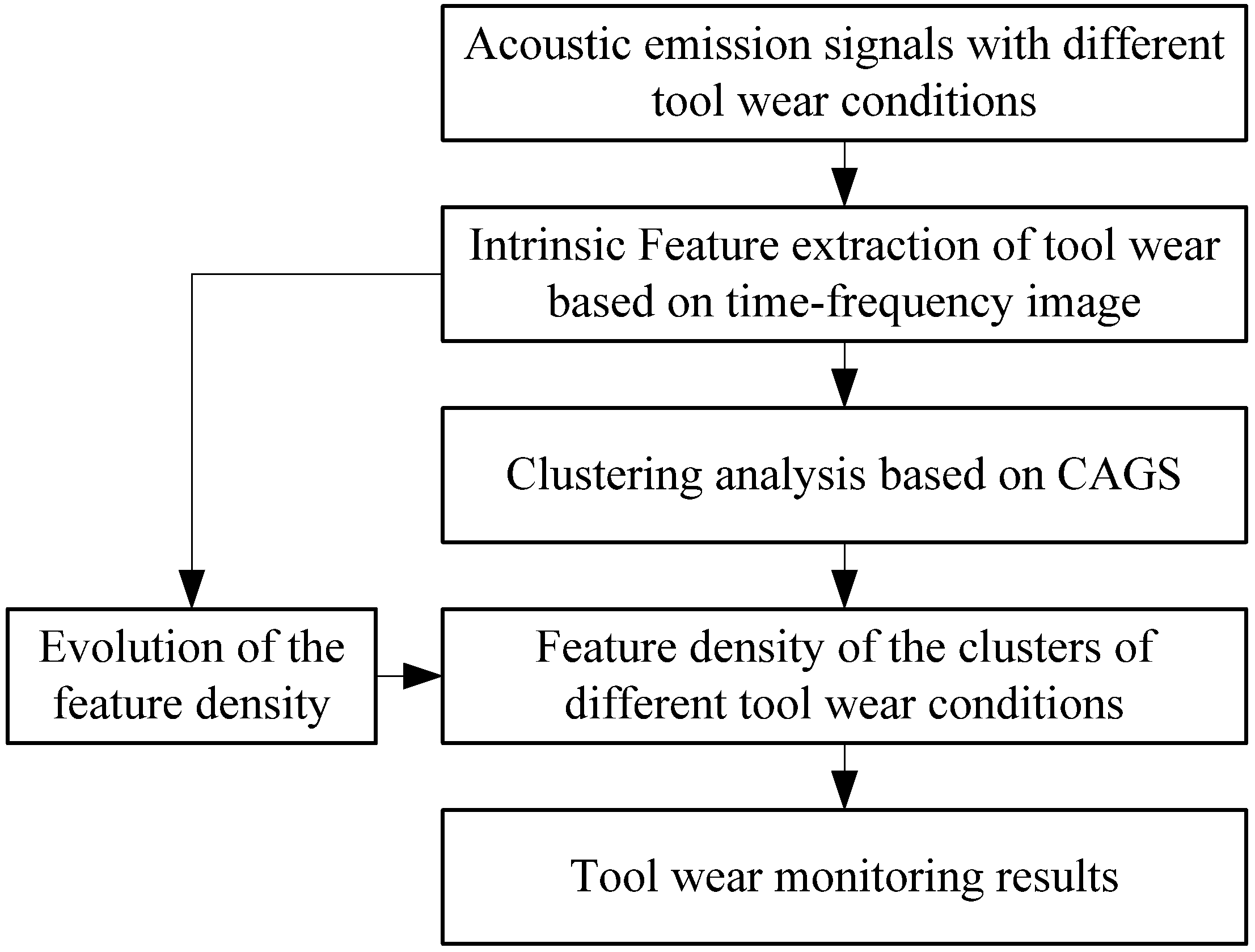
To realize tool wear monitoring in corner milling, an unsupervised state framework is constructed in this paper, as shown in Figure 1. First, AE signals are collected during corner milling under different tool wear conditions. Then the intrinsic features of the tool wear condition are extracted from the time–frequency image of the AE signal to form a sample space containing the tool wear information. A clustering algorithm based on adjacent grid search (CAGS) was used to divide the samples into several clusters with different distributions, and the feature density of the clusters was calculated. By analyzing the feature distribution under different tool wear conditions, the evolution law of feature density can be obtained. Finally, tool wear can be identified by the density factor proposed in this paper.

2.2. Intrinsic Feature Extraction Based on Time-Frequency Image

2.2.1. Multi-Resolution Analysis of Acoustic Emission Signals

The acoustic emission sensor can simultaneously collect the high frequency and low frequency information in the cutting process, but the frequency response characteristics of the sensor determine that only the specific frequency band information is effective. In this paper, the signal is decomposed into different scales or frequency bands through multi-resolution analysis. The acoustic emission signal is decomposed using a discrete wavelet transform method. The following formula can be used to reconstruct signal $s\left(t\right)$ using wavelet series:

$$s\left(t\right)={\displaystyle \sum }_{j,k\in Z}\langle s\left(t\right),{\mathsf{\psi }}_{j,k}\left(t\right)\rangle {\psi }^{j,k}\left(t\right)={\displaystyle \sum }_{j,k\in Z}{C}_{j,k}\left(t\right){\psi }^{j,k}\left(t\right)$$

(1)

where ${\mathsf{\psi }}_{j,k}\left(t\right)$ is a set of wavelet frames, ${\psi }^{j,k}\left(t\right)$ is the dual wavelet framework of ${\mathsf{\psi }}_{j,k}\left(t\right)$. Because this reconstruction is redundant in most cases, this paper uses MALLT algorithm to realize the binary discrete decomposition of the original signal.

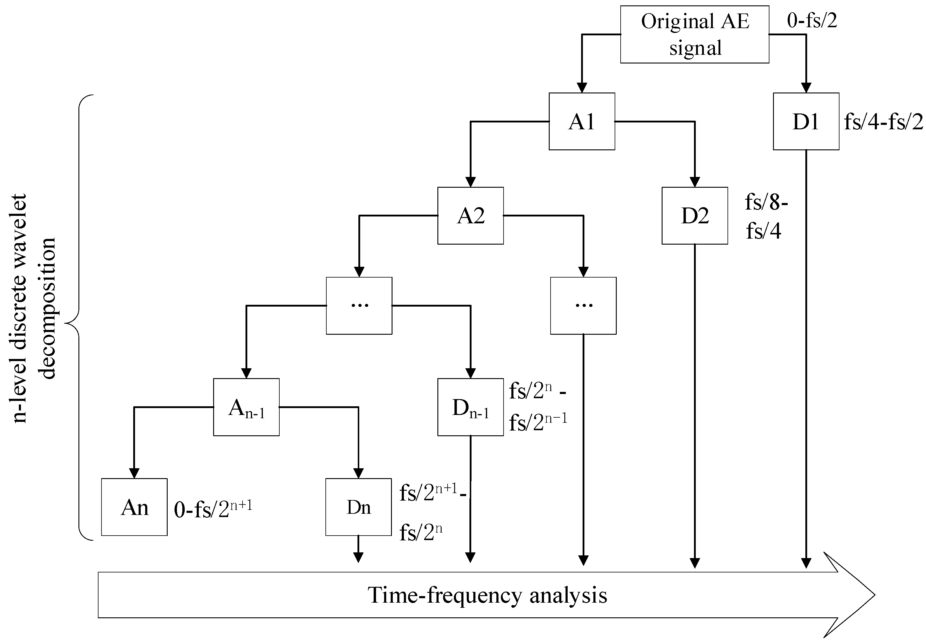
For a sequence of AE signals with a sampling frequency of $f_s$, the binary discrete wavelet decomposition process is shown in Figure 2.

After each layer of discrete wavelet decomposition, the signal is evenly divided into two parts in terms of frequency, and the wavelet coefficient of the high-frequency part is denoted as D; the wavelet coefficient of the low-frequency part is denoted as A. Then, time-frequency analysis is performed on each signal component separately.

2.2.2. Time-Frequency Analysis of AE Signal Based on Short-Time Fourier Transform (STFT)

The signal can be roughly decomposed to different scales by discrete wavelet decomposition. In order to further characterize the time-frequency characteristics of the signal, it is necessary to decompose the time-domain waveform of the signal into two-dimensional time–frequency plane through an effective time-frequency analysis method. Among many time–frequency analysis methods, STFT can not only suppress energy leakage but also perform well in time resolution and computational efficiency. Therefore, this paper uses STFT for analysis of cutting AE signals. The mathematical expression for the STFT is:

$$STFTs\left(t_s,f\right)={{\displaystyle \int }}_{-\infty }^{+\infty }[x\left(\tau \right)r^{*}\left(\tau -t\right)]e^{-j2\pi ft}dt$$

(2)

where $s\left(t\right)$ is a non-stationary original signal, $r^{*}\left(\tau -t\right)$ is the window function.

The time–frequency diagram of the AE signal can reflect the non-stationarity of the cutting process to a certain extent, but it is clearly affected by the acoustic emission energy. In this paper, the time–frequency image is normalized to remove the factors of energy changing with time from the time–frequency diagram and obtain the time-varying information that only reflects the frequency component in the cutting state. Assuming the discrete signal sequence $s\left(n\right)$ passes STFT, the time–frequency matrix obtained is $P\left[n,k\right]$. For column $i$ of $P\left[n,k\right]$, $P\left[n,k\right]$ is normalized according to the following method:

$$P\left[n,k\right]=\frac{\left(P\left[n,k\right]-P_{min}\left[n,k\right]\right)\times 2}{P_{max}\left[n,k\right]-P_{min}\left[n,k\right]}-1$$

(3)

All columns of $P\left[n,k\right]$ are normalized to obtain normalized time–frequency matrix $P\left[n,k\right]$.

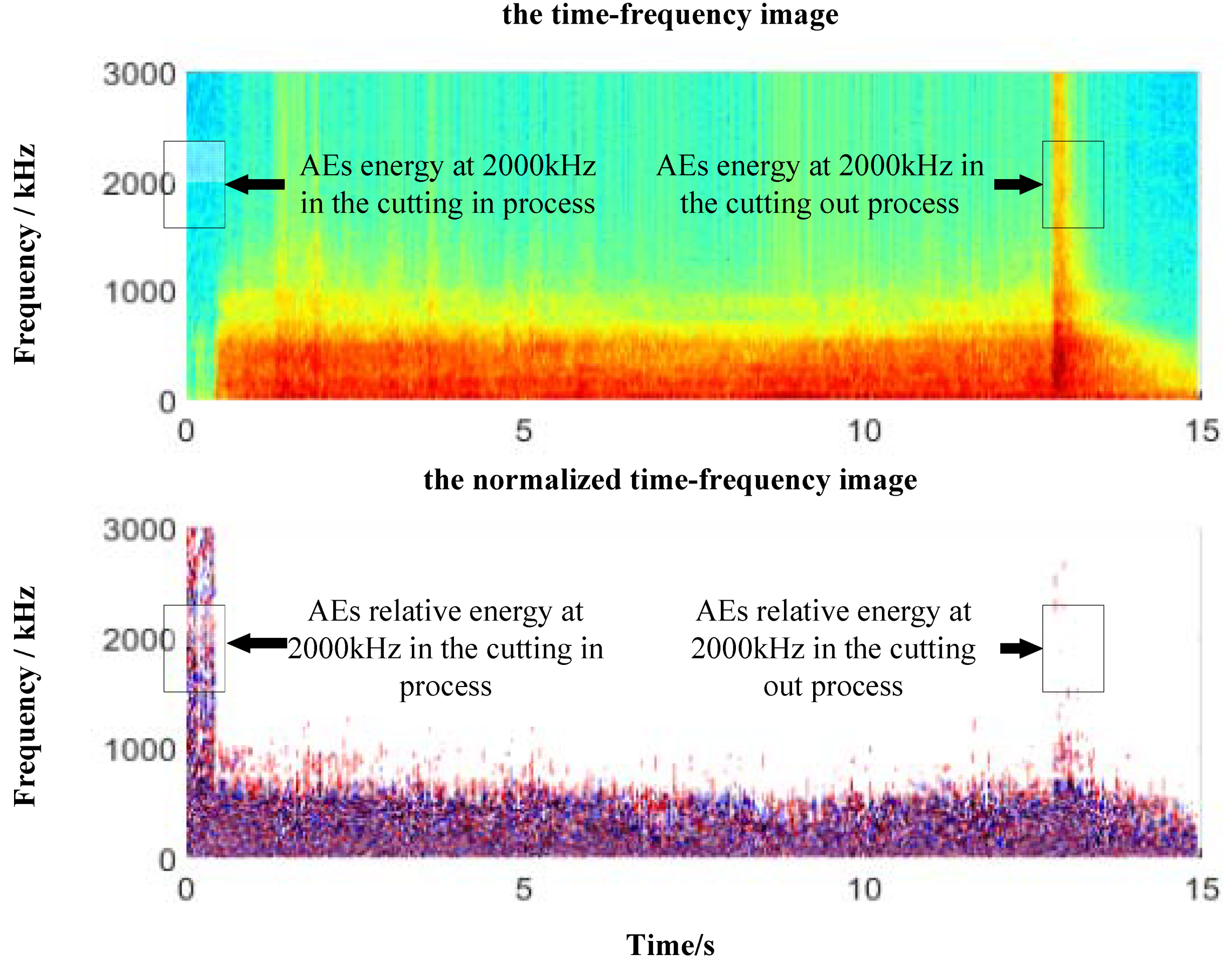
The normalized time-frequency image is shown in Figure 3. In the time-frequency image, the AEs’ energy at 2000 kHz in the cutting in process is smaller than that in the cutting out process. On the contrary, in the normalized time–frequency image, the AEs’ relative energy at 2000 kHz in the cutting in process is larger than that in the cutting out process. Therefore, it can be seen that the normalized time spectrum is not affected by the energy of acoustic emission signal and can directly reflect the change I the instantaneous frequency component of the acoustic emission signal with time.

2.2.3. Feature extraction

After obtaining the time–frequency image and normalized time–frequency image of acoustic emission signal, it is necessary to extract the features based on the time–frequency image. The characteristics of the time–frequency diagram include energy characteristics, time–domain and frequency-domain expansion characteristics and time–frequency intrinsic characteristics.

Energy characteristics: The time–frequency information of the signal is obtained by analyzing the energy distribution characteristics in the time–frequency image. It includes the energy of a specific frequency band, the total energy and the statistical characteristics of the time–frequency diagram compressed along the time axis or the frequency axis, as shown in

Table 1. Energy characteristics of the time–frequency diagram.

Energy Characteristics	Expression
Specific frequency band energy	$E{B}_{\left(t,f\right)}={\displaystyle \sum _{k=\left[\left(i-1\right)\mathsf{∆}+1\right]}^{\left[i\mathsf{∆}\right]}}P\left[n,k\right]$
total energy	$E_{\left(t,f\right)}={\displaystyle \sum _{n=1}^N}{\displaystyle \sum _{k=1}^M}P\left[n,k\right]$

and

Table 2. Statistical characteristics of the compressed time–frequency matrix along the time axis or the frequency axis.

Distribution over Time	Expression	Distribution with Frequency	Expression
variance	${\widehat{\sigma }}_t^2=var\left(P_t\left[n\right]\right)$	variance	${\widehat{\sigma }}_f^2=var\left(P_f\left[k\right]\right)$
skewness	${\widehat{\gamma }}_t=ske\left(P_t\left[n\right]\right)$	skewness	${\widehat{\gamma }}_f=ske\left(P_f\left[k\right]\right)$
kurtosis	${\widehat{k}}_t=kur\left(P_t\left[n\right]\right)$.	kurtosis	${\widehat{k}}_f=kur\left(P_f\left[k\right]\right)$
		peak frequency	${\widehat{f}}_{P{f}_{max}}=F\left(\left[P_{f_{max}}\right]\right)$
		Frequency center of gravity	${\widehat{f}}_m=\frac{{{\displaystyle \sum }}_{k}F\left[k\right]P_f\left[k\right]}{M}$

.

The time–frequency diagram is a two-dimensional matrix. The distribution of time–frequency energy with time can be obtained by summing the coefficients of each column:

$$P_t\left[n\right]={{\displaystyle \sum }}_{k}P\left[n,k\right]$$

(4)

Sum the coefficients of each row separately to obtain the distribution of time–frequency energy with frequency:

$$P_f\left[k\right]={{\displaystyle \sum }}_{n}P\left[n,k\right]$$

(5)

Both distributions are one-dimensional vectors, for which statistical features are extracted separately, as shown in Table 2.

Time-domain and frequency-domain expansion features: Time domain features are based on the basic assumption that there are different probability distributions between normal signals and abnormal signals and that the characterization of monitoring targets is realized by extracting the statistical features of signals. The common time-domain characteristics are usually for one-dimensional signals. If the time-frequency image is regarded as a two-dimensional signal, the time-domain expansion characteristics of the time–frequency diagram can be obtained. This paper gives some extended features corresponding to common time–frequency features, as shown in

Table 3. Time-domain expansion features of the time–frequency matrix.

Time Domain Expansion Characteristics	Expression
mean value	$m_{\left(t,f\right)}=\frac{1}{NM}{\displaystyle \sum }_n{\displaystyle \sum }_{k}P\left[n,k\right]$
variance	${\sigma }_{\left(t,f\right)}^2=\frac{1}{NM}{\displaystyle \sum }_n{\displaystyle \sum }_k{\left(P\left[n,k\right]-m_{\left(t,f\right)}\right)}^2$
skewness	${\gamma }_{\left(t,f\right)}=\frac{1}{\left(NM-1\right){\sigma }_{\left(t,f\right)}^3}{\displaystyle \sum }_n{\displaystyle \sum }_k{\left(P\left[n,k\right]-m_{\left(t,f\right)}\right)}^3$
kurtosis	${\kappa }_{\left(t,f\right)}=\frac{1}{\left(NM-1\right){\sigma }_{\left(t,f\right)}^4}{\displaystyle \sum }_n{\displaystyle \sum }_k{\left(P\left[n,k\right]-m_{\left(t,f\right)}\right)}^4$
coefficient of variation	$c_{\left(t,f\right)}=\frac{{\sigma }_{\left(t,f\right)}}{m_{\left(t,f\right)}}$

. When it is necessary to distinguish between two different signals with a similar frequency spectrum, it is solved by expanding the frequency domain features to the time–frequency domain.

Table 4. Frequency-domain expansion characteristic of the time–frequency matrix.

Frequency-Domain Expansion Features	Expression
Spectral flux	$F{L}_{\left(t,f\right)}={\displaystyle {\displaystyle \sum }_{n=1}^{N-1}}{\displaystyle {\displaystyle \sum }_{K=1}^{M-m}}\left|P\left[n+l,k+m\right]-P\left[n,k\right]\right|$
Spectral entropy	$R{E}_{\left(t,f\right)}=\frac{1}{1-\alpha }{\log }_2{\displaystyle {\displaystyle \sum }_{n=1}^N}{\displaystyle {\displaystyle \sum }_{K=1}^M}{\left(\frac{P\left[n,k\right]}{{{\displaystyle \sum }}_n{{\displaystyle \sum }}_{k}P\left[n,k\right]}\right)}^{\alpha }$
Spectrum flatness	$S{F}_{\left(t,f\right)}=MN\frac{{{\displaystyle \prod }}_{n=1}^N{{\displaystyle \prod }}_{k=1}^{M}P\left[n,k\right]}{{{\displaystyle \sum }}_{n-1}^N{{\displaystyle \sum }}_{k=1}^{M}P\left[n,k\right]}$

shows some common frequency-domain features and corresponding extended features.

Time–frequency intrinsic features: Some features are essentially time–frequency features, which cannot be defined in the time domain or the frequency domain, that is, the intrinsic features of a time–frequency image. In this paper, the intrinsic characteristics and their expressions based on a time–frequency diagram are given in

Table 5. The intrinsic characteristics of the time–frequency diagram.

Time Frequency Internal Characteristics	Expression
Maximum singular value	$ms{v}_{\left(t,f\right)}=\max \left({\overline{s}}_1,\cdots ,{\overline{s}}_N\right)$
Complexity measurement	$C{M}_{\left(t,f\right)}=-{\displaystyle {\displaystyle \sum }_{i=1}^N}{\overline{s}}_i{\log }_2{\overline{s}}_i$
Transient frequency deviation	$di{f}_{\left(t,f\right)}=\max \left(if\left[n\right]\right)-\min \left(if\left[n\right]\right)$
Time frequency concentration	$M_{\left(t,f\right)}={\left({\displaystyle {\displaystyle \sum }_{n=1}^N}{\displaystyle {\displaystyle \sum }_{k=1}^M}{\left|P\left[n,k\right]\right|}^{1/2}\right)}^2$

.

2.3. Unsupervised Feature Selection Based on Trend Item Analysis

The initial feature set obtained after feature extraction is of high dimension and contains a large number of redundant features. Therefore, the initial feature set should be dimensionally reduced before feature selection. This paper uses the cross-correlation coefficient to achieve feature dimension reduction. For example, for two eigenvectors $f_1$ and $f_2$, the number of interrelations between them is:

$$r\left(f_1,f_2\right)=\left|\frac{Cov\left(f_1,f_2\right)}{\sqrt{var\left(f_1\right)var\left(f_2\right)}}\right|$$

(6)

where $Cov\left(f_1,f_2\right)$ is the covariance of the two features. The greater the number of correlations, the greater the linear correlation between the two features. When $r=1$, the information contained in $f_1$ and $f_2$ is the same. The main steps of feature dimensionality reduction using correlation numbers are as follows:

• Calculate the cross-correlation coefficient between each feature and other features in the initial feature set S to obtain the correlation number matrix $\mathrm{R}{\left(\mathrm{i},\mathrm{j}\right)}_{\mathrm{i},\mathrm{j}}\le \mathrm{n}$, where $\mathrm{n}$ is the number of features.
• Set a threshold T to calculate the number N(i) which denotes the number of relevant features of the ith feature f_i. If the cross-correlation coefficient of two features exceeds T, they are considered as relevant feature with each other.
• Find the feature having the largest N and set it as the main feature f_m. Establish a new self-similarity feature set S_i(c) by extracting all the relevant features of f_m from S.
• For all the other features except f_m in S_i(c), find their relevant features in S and the N(i) of their relevant features minus one. The number of self-similarity feature set plus one.
• Repeat steps 3–4 until the maximum N(i) in S is 0. Then, establish a self-similarity feature set for each feature, if have, remaining in S.
• Collect the main features of all self-similarity feature sets to form the dimension-reduced feature set S_opt.

According to the above steps, the initial feature set can be reduced into several main features, realizing the initial feature dimension reduction.

In this paper, a method based on feature trend term analysis is used for feature selection. If a feature vector reflecting tool wear state is regarded as a one-dimensional signal, it is mainly composed of a trend term and a fluctuation term. The trend term usually reflects the change trend of the monitoring target and should have good linearity; the fluctuation term is usually disturbed by the signal by external noise; the stronger the fluctuation term, the worse the robustness of the feature. The effectiveness of the feature vector is evaluated by the following formula:

$$LER=\frac{r^p\left(f_{lin},f_{tre}\right)}{E_{wave}}$$

(7)

where p is balance parameters, $E_{wave}$ is volatility term energy, $f_{tre}$ is trend term and $f_{lin}$ is a linear vector of the construction.

2.4. Unsupervised Clustering Algorithm Based on Adjacent Grid Search

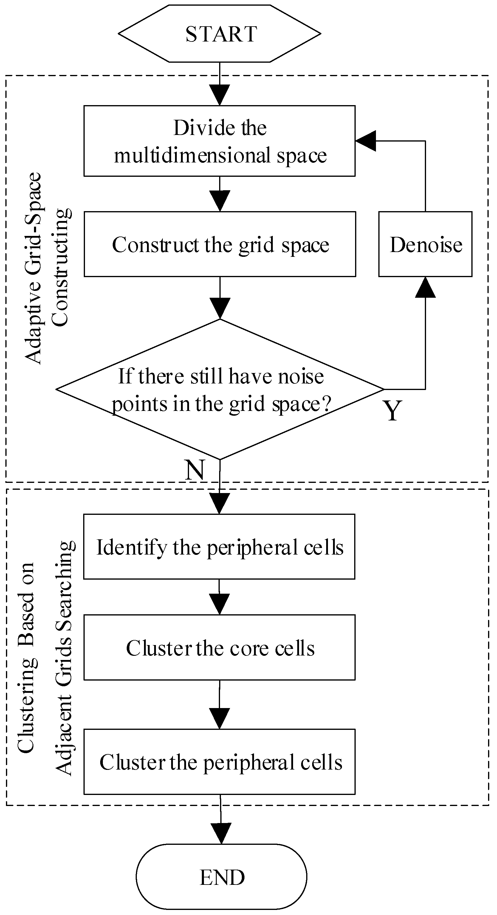
During the milling of large aviation structural parts, due to the lack of off-line testing to provide necessary prior knowledge, unsupervised pattern recognition has become a priority, and clustering is a commonly used unsupervised pattern recognition algorithm. In this paper, a clustering algorithm based on adjacent grid search (CAGS) is established. This algorithm can automatically identify the number of clusters, find clusters of arbitrary shape, process noise data, process high-dimensional data, process large-scale data and minimize a priori knowledge. The algorithm flow is shown in Figure 4.

A multidimensional space $S^d$ is composed of multiple orthogonal continuous dimensions. A sample point set $D^d$ is distributed in $S^d$:

$$D^d=\left\{D_1^d,D_2^d,\cdots ,D_d^d\right\}$$

(8)

where $D_i^d\subset S_i^d$ is the x-dimensional distribution state of $D^d$ in $S^d$. Usually, multidimensional sample sets are discrete, finite and uneven. The multidimensional sample set also has another representation:

$$D^d=\left\{X_1^d,X_2^d,\cdots ,X_N^d\right\}$$

(9)

where N is the sample set size, the total number of samples in the sample set, and $X_i^d$ is the $i$th sample in $D^d$. The distribution of the sample set in $S^d$ identifies a finite d-dimensional space, which is gridded using a monotonic scale sequence, the expression is as follows:

$$S{C}_i^D=\left\{S{C}_i^D\left(0\right),S{C}_i^D\left(1\right),\cdots ,S{C}_i^D\left(k\right)\right\}$$

(10)

where $S{C}_i^D\left(k\right)$ represents the $k+1$st hyperplane in the ith dimension in a finite d-dimensional space. The multidimensional grid space generated after the multidimensional space segmentation is expressed as:

$$G^D=\left\{C_1^D,C_2^D,\cdots ,C_i^D\right\}$$

(11)

where $C_i^D$ is the $i$th cell in grid space $G^D$ and each cell is a super rectangle in $G^D$. At the same time, cell $C_i^D$ also has the following attribute values:

$$C_i^D=\left\{location,member,density\right\}$$

(12)

where location is the coordinate of the cell in the grid space; member is a member of a cell, that is, a set of sample points within the cell; and density is the density value of the cell, that is, the number of sample points within the cell range.

After the above steps, we will treat the grid as follows:

• Kill (delete) all empty cells with density of 0;
• Realign all the remaining non-empty cells from large to small by density;
• Set glow threshold $threH$ and define the cells with a density less than that threshold as the halo cells; define the density Cells greater than or equal to this threshold as core cells. The halo threshold is calculated by the following equation:

  $$threH=\frac{{{\displaystyle \sum }}_{i=1}^{M}density\left(C_i^D\right)}{M}{f}_H$$

  (13)

  where $f_H$ is the halo coefficient and M is the total number of cells.

In this paper, an adjacent grid search method is used to realize grid clustering. In a multidimensional grid space $G^D$ constructed for a multidimensional sample set $D^d$, the cell coordinates adjacent to a cell $C_i^D$ can be obtained by the following equation:

$$location\left(A{C}_i^D\right)=location\left(C_i^D\right)+Aop{t}^d$$

(14)

where $A{C}_i^D$ is the adjacent cell of $C_i^D$, also known as adjacent grid. $Aop{t}^d$ is a d-dimensional adjacent operator:

$$Aop{t}^d=\left\{L_1^d,L_2^d,\cdots ,L_T^d\right\}-0$$

(15)

where $L_{T }$ is the d-dimensional coordinate vector arranged in a symmetric triad in ascending order. $T=3^d$, the symbol “$-$” represents the set seeking the difference, and 0 represents a d-dimensional null vector.

The formal clustering process falls into two stages: traversal of core cells and processing of halo cells.

In the first stage, the cells sorted by density are traversed successively to find the core of each cluster. The traversal process follows the following principles:

• Take a new cell each time and judge whether it belongs to an existing cluster; if it does not, it is defined as a new cluster, and otherwise, the next cell is processed.
• First, for a newly defined class cluster, the adjacent cells of the cell creating the class cluster are found in the core cell; these are classified as this class cluster. Then, cycle through the cells in the cluster and classify the adjacent cells belonging to them in the core cell as the cluster until no new cells are included.

In the second stage, each halo cell is assigned to the nearest adjacent cell cluster based on the nearest cell principle. However, for a halo cell, there may be two scenarios: adjacent cells and no adjacent cells. When an adjacent cell exists, the distance between it and the adjacent cells is calculated separately: In that case, find the nearest adjacent cells, judge the cluster to which the nearest adjacent cell belongs and classify the halo cells into the cluster. If a halo cell does not have adjacent cells, the halo cell is defined as a new cluster.

Finally, after all the halo cells are processed, the clustering is complete.

2.5. Analysis of the Clustering Results Based on Cluster-Like Density Factors

The monitoring of tool wear belongs to the condition monitoring problem of monotonic multi classification. Its characteristic is that the eigenvalue of the monitoring signal basically changes continuously and monotonically with the degree of tool wear. However, through a large number of studies, we found that in addition to using the change in eigenvalue size, we use the distribution state information of samples in the feature space to reflect the evolution law of monitoring targets. For example, in the process of increasing tool wear, not only does the amplitude of cutting force increase, but the divergence of features increases; that is, the more serious the tool wear, the sparser the corresponding cluster sample distribution. The divergence of the sample distribution is more universal than the change law of the eigenvalue size. For some features, the opposite rule may also occur, that is, the wear samples are more densely distributed than the normal samples.

In this paper, a tool wear state identification method based on cluster density factor is used to analyze the clustering results. The density factor can be calculated by the following formula:

$$War\left(i\right)=\frac{density\left(i\right)-densit{y}_0}{densit{y}_0·T}$$

(16)

where $War\left(i\right)$ is the density factor of the $i$th class found in the clustering process, and its size increases with increasing wear. $densit{y}_0$ is the mean sample density of the class cluster with the smallest density, density(i) is the mean sample density of the $i$th class cluster identified by the clustering algorithm during the monitoring process and T is the fault truncation coefficient. The greater T is, the higher the tolerance of tool wear is.

2.6. Evaluation of the Effectiveness of the Clustering Results

In this paper, the effectiveness of recognition results is evaluated by using the following five metrics:

• Purity [23]:

$$PUR=\frac{1}{n}{{\displaystyle \sum }}_{k^A}{n}_{k^C,k^A} , k^C=k^A$$

(17)

2.

Cluster similarity [24]:

$$CSM=\frac{1}{k^A}{{\displaystyle \sum }}_{k^A}\underset{1\le k^C\le K^C}{\max }\frac{2n_{k^C,k^A}}{n_{k^C}+n_{k^A}}$$

(18)

3.

Normalized mutual information [25]:

$$NMI=\frac{{{\displaystyle \sum }}_{k^A}{{\displaystyle \sum }}_{k^C}{n}_{k^C,k^A}\log \frac{n·n_{k^C,k^A}}{n_{k^C}·n_{k^A}}}{\sqrt{\left({{\displaystyle \sum }}_{k^A}{n}_{k^A}\log \frac{n_{k^A}}{n}\right)\left({{\displaystyle \sum }}_{k^C}{n}_{k^C}\log \frac{n_{k^C}}{n}\right)}}$$

(19)

4.

Cluster-based cross entropy [23]:

$$CluCE=\frac{-{{\displaystyle \sum }}_{k^C}\frac{n_{k^C}}{n}{{\displaystyle \sum }}_{k^A}\frac{n_{k^C,k^A}}{n_{k^C}}\log \frac{n_{k^C,k^A}}{n_{k^C}}}{\log K^A}$$

(20)

5.

Class-based cross entropy [23]:

$$ClaCE=\frac{-{{\displaystyle \sum }}_{k^A}\frac{n_{k^A}}{n}{{\displaystyle \sum }}_{k^C}\frac{n_{k^C,k^A}}{n_{k^A}}\log \frac{n_{k^C,k^A}}{n_{k^A}}}{\log K^C}$$

(21)

In the above five formulas, $k^C\in \left\{1,2,\cdots ,k^C\right\}$ represents the category obtained after clustering, $k^A\in \left\{1,2,\cdots ,k^A\right\}$ represents the real category of the sample set,$n$ represents the total number of samples in the sample set, $n_{k^C}$ represents the total number of samples of class $k^C$ in the clustering results, $n_{k^A}$ represents the total number of samples of class $k^A$ in the clustering results, and $n_{k^C,k^A}$ represents the number of intersections between class $k^C$ samples in the clustering results and class $k^A$ samples in the sample set.

3. Experiments

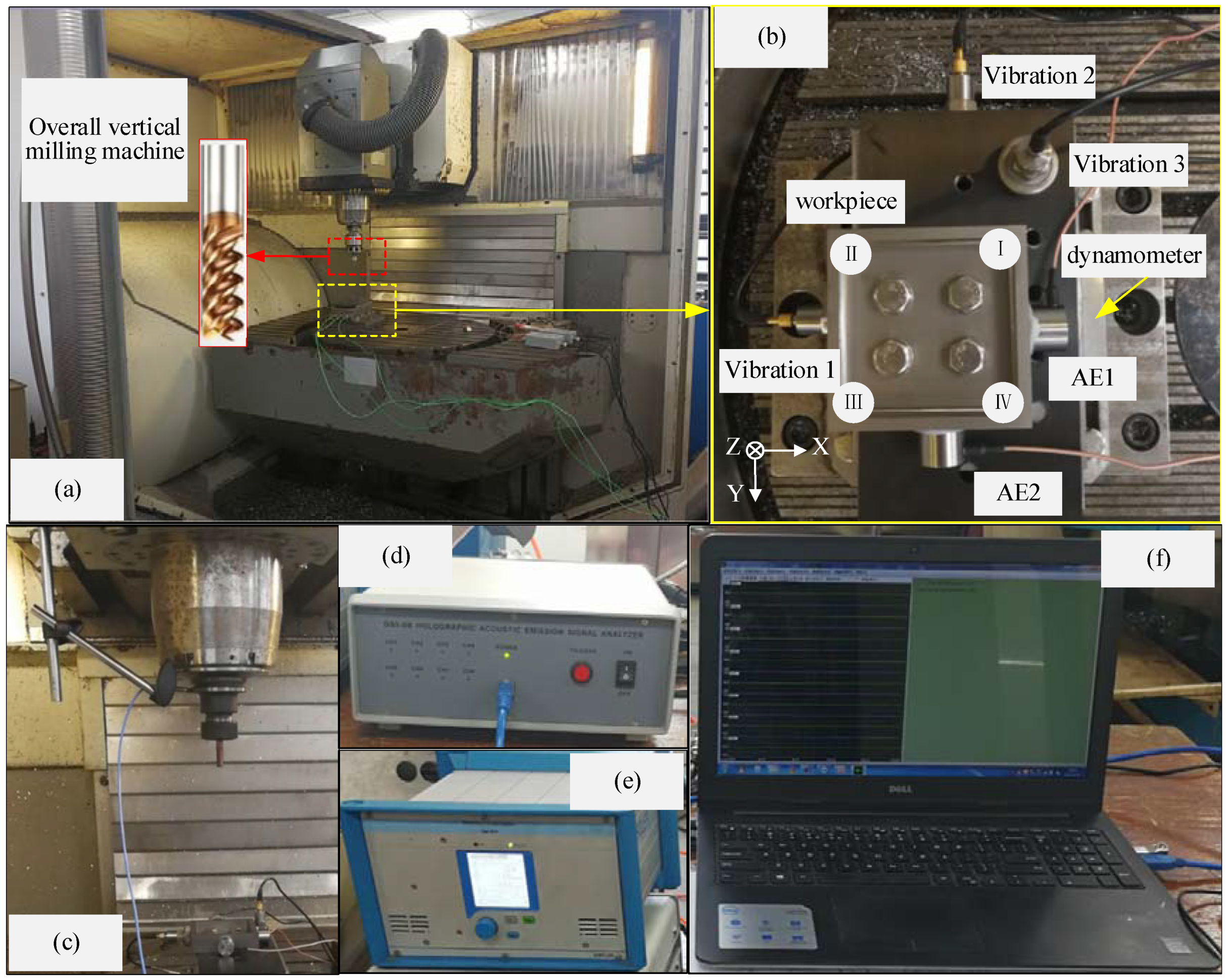
In this paper, to verify the proposed micro-wear monitoring method for the tool in the machining of the corner features of aeronautical structural part, a metal cutting condition monitoring platform based on the synchronous acquisition of multi-sensor information is built as shown in Figure 5. The platform can simultaneously collect up to eight channels of acoustic emission signals and eight channels of external parameter signals. The highest sampling frequency of acoustic emission signals can reach 6 MHz, and the highest sampling frequency of external parameter signals can reach 40 kHz. In this corner fine-milling experiment, 2 channels of acoustic emission signals are configured, and the sampling frequency is 3 MHz. The external parameter signals are configured with 3 channels of cutting force signals, 3 channels of vibration signals and 1 channel of key phase signals, and the sampling rate is 30 kHz. The key phase signal can be used to determine the periodic calculation of the cutting and cutting angles of the cutter teeth.

The milling experiment was carried out on a five-axis Demag CNC machining center (model: DMU80T); the linear displacement error was 0.001 mm, and the maximum spindle rotation concentricity was less than 0.02 mm, which met the requirements of fine milling. The workpiece is a square groove with a wall thickness of 5 mm, the inner wall size is 70 mm, and the groove depth is 10 mm, including 4 corners, which are corner I, corner II, corner III and corner IV in order of processing. The machining radius of each corner is 8 mm. The workpiece is directly fixed on the dynamometer, and the dynamometer is fixed on the machine tool through a vise. The workpiece material is selected from the most widely used titanium alloy TC4 in the industry.

Table 6. Physical and mechanical properties of TC4 at ambient temperature.

Material Composition	Thermal Conductivity (W·m−1 ·K−1)	Tensile Strength (MPa)	Yield Strength (MPa)	Elastic Modulus (GPa)	Hardness (HB)
Ti-6Al-4V	8.37	993	830	114	36

is the material parameter attribute table. Due to the rapid wear and tear of titanium alloy materials on the tool, this experiment uses a special alloy tool for titanium alloy, model UTH0804.

Table 7. Specific parameters for corner milling tools.

UTH0804	Diameter D (mm)	Overall Length L (mm)	Blade Length L1 (mm)	Number of Teeth N	Helical Angle β (°)
	8	60	20	4	52

shows the detailed parameters of the tool.

In this experiment, the spindle speed of the corner milling is 5000 r/min, the converted cutting speed is 125.6 m/min, the axial depth of cut is 4 mm, the radial depth of cut is 0.1 mm, the feed per tooth is 0.02 mm/tooth, and the milling method is down milling. The starting point of the path is the straight line between corner I and corner IV (the position corresponding to the acoustic emission sensor AE1 in Figure 5), and the tool moves in a counterclockwise direction. The four workpieces shown in Figure 5 are machined continuously with the same milling cutter. After each machining, the flank wear values of the four teeth were measured, as shown in

Table 8. The wear values of the experimental tool for corner circumferential milling.

Metrics	Workpiece Serial Number	Cutter Tooth A	Cutter Tooth B	Cutter Tooth C	Cutter Tooth D	Standard Value
$VB$(mm)	1	0.03	0.02	0.03	0.02	0.025
	2	0.06	0.05	0.06	0.04	0.053
	3	0.08	0.09	0.08	0.06	0.078
	4	0.10	0.09	0.10	0.07	0.09
$V{B}_{max}$(mm)	1	0.08	0.12	0.15	0.18	0.18
	2	0.15	0.17	0.17	0.24	0.24
	3	0.18	0.20	0.23	0.26	0.26
	4	0.21	0.23	0.26	0.27	0.27

. According to the definition in ISO8688-2, the average value of the flank wear band is taken as worn VB, and the maximum value of the wear band is taken as worn $V{B}_{max}$. According to the standard, when $VB$ reaches or exceeds 0.3 mm or $V{B}_{max}$ reaches or exceeds 0.5 mm, the tool life limit is considered to be reached.

4. Results and Discussion

4.1. Non-Stationary Characteristics of Corner Milling

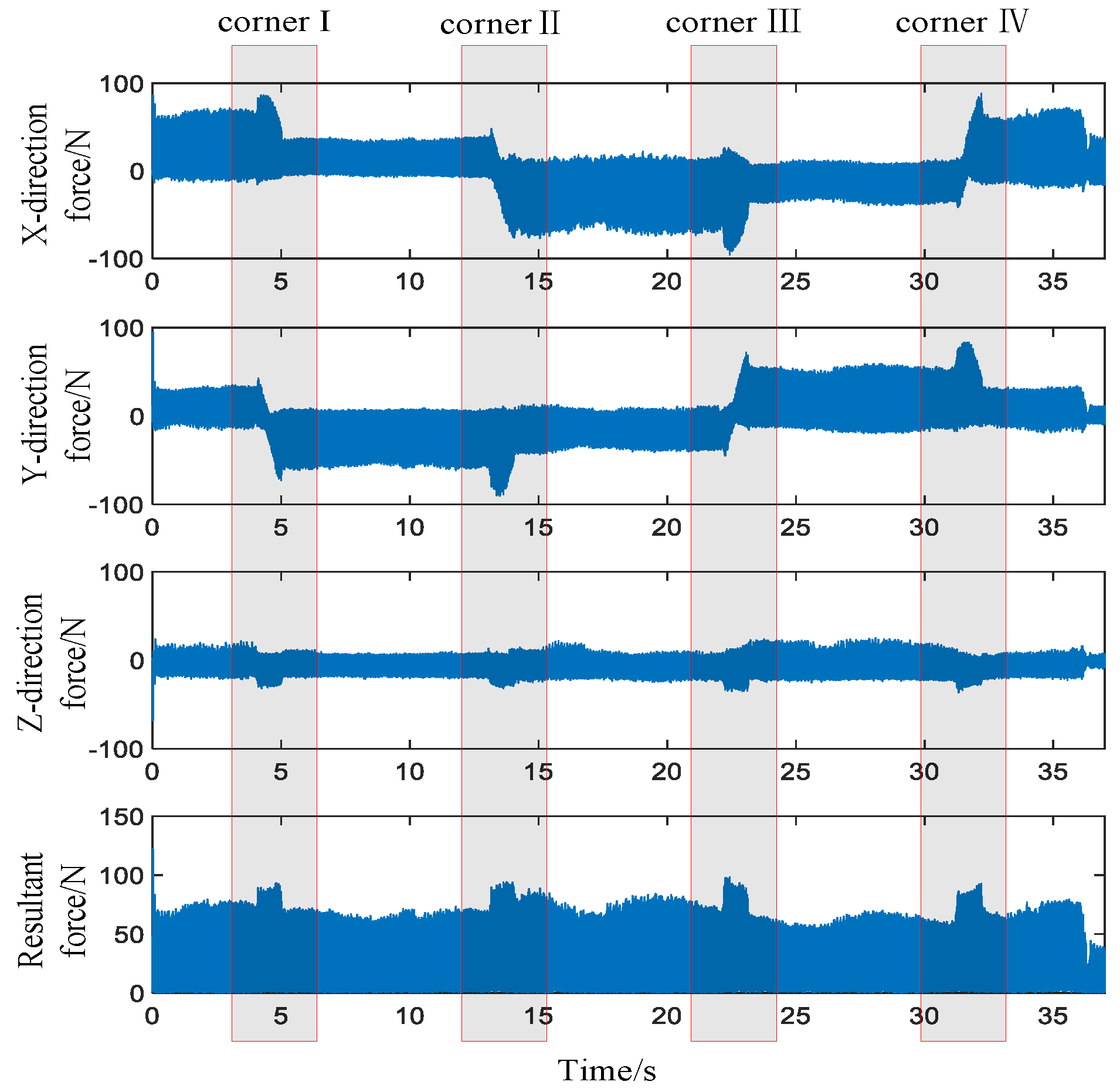
When cutting parameters such as cutting width, depth of cut and feed rate remain unchanged, changes in the tool path will lead to significant changes in cutting force caused by the special shape at the corners. The average cutting force will increase when the machined surface is concave along the tool side, and the average cutting force will decrease when the machined surface is convex along the tool side. Since the cutting amount of the tool to the workpiece, the angle of the tool axis and the tool path are constantly changing with the machining process, the sensor signal shows a highly non-stationary characteristic.

It can be seen from Figure 6 that in the curve section of each corner, the cutting force changes rapidly, and the maximum amplitude is significantly higher than that of the straight section. The non-stationarity of the cutting force in the straight segment can be eliminated to a certain extent by calculating the resultant force of the forces in all directions, but it is invalid at the corners. Therefore, for corner milling, the cutting force is highly non-stationary. It can be seen from Figure 7 that the system stiffness of the tool in the corner section is significantly greater than that in the straight section, resulting in significantly smaller vibration signals in the corner section than in the straight section. The vibration signals in the three directions all show strong non-stationary characteristics with the cutting path. 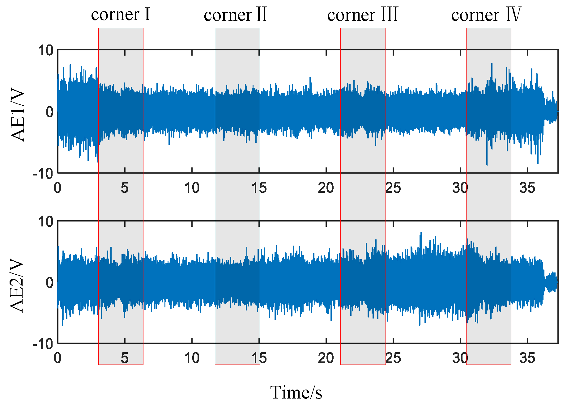It can be seen from Figure 8 that the time-domain waveform of the acoustic emission signal is far less sensitive to the path than the cutting force signal and the vibration signal.

To sum up, both the force signal and the vibration signal show strong non-stationary characteristics with the corner milling path, while the corner milling path has little influence on the acoustic emission signal. Therefore, compared with the other two sensor signals, the acoustic emission signal has a great advantage in monitoring corner milling.

4.2. The Effectiveness of Time-Frequency Images for Characterizing Tool Wear

By observing the data of tool wear evolution in Table 8, it can be found that the tool wear gradually increased, and the wear rate showed a gradually smaller trend in the four cuts. Therefore, the features that can effectively characterize the tool wear state should also have the same trend of change.

After extracting the time–frequency features using the tool wear monitoring feature extraction method of corner milling, a 6 × 84-dimensional high-dimensional characteristic matrix. In order to obtain the optimal low-dimensional effective feature set, firstz unsupervised feature dimensionality reduction was carried out using the feature dimensionality reduction method based on correlation number. Then, the filtered feature selection method based on trend term analysis was used to further optimize the non-redundant feature set to extract the first six-dimensional optimal features, as shown in

Table 9. The optimal feature set of acoustic emission for the wear of corner peripheral milling tools.

Feature Serial Number	Feature Name	Wavelet Number	LER6
1	Raney entropy	5	121.8
2	Maximum singular value	0	100.1
3	Raney entropy	1	83.2
4	Maximum singular value	2	50.7
5	Raney entropy	2	37.8
6	Complexity measurement	1	26.1

. As can be seen from the table, the most effective six-dimensional features are the time–frequency intrinsic features presented in this paper, two of which are extracted based on the normalized time–frequency image.

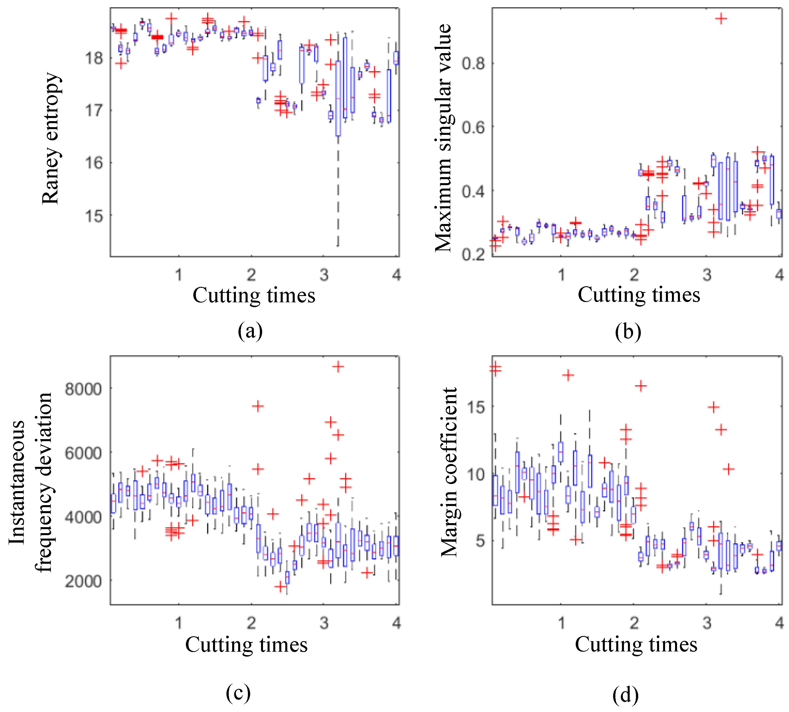
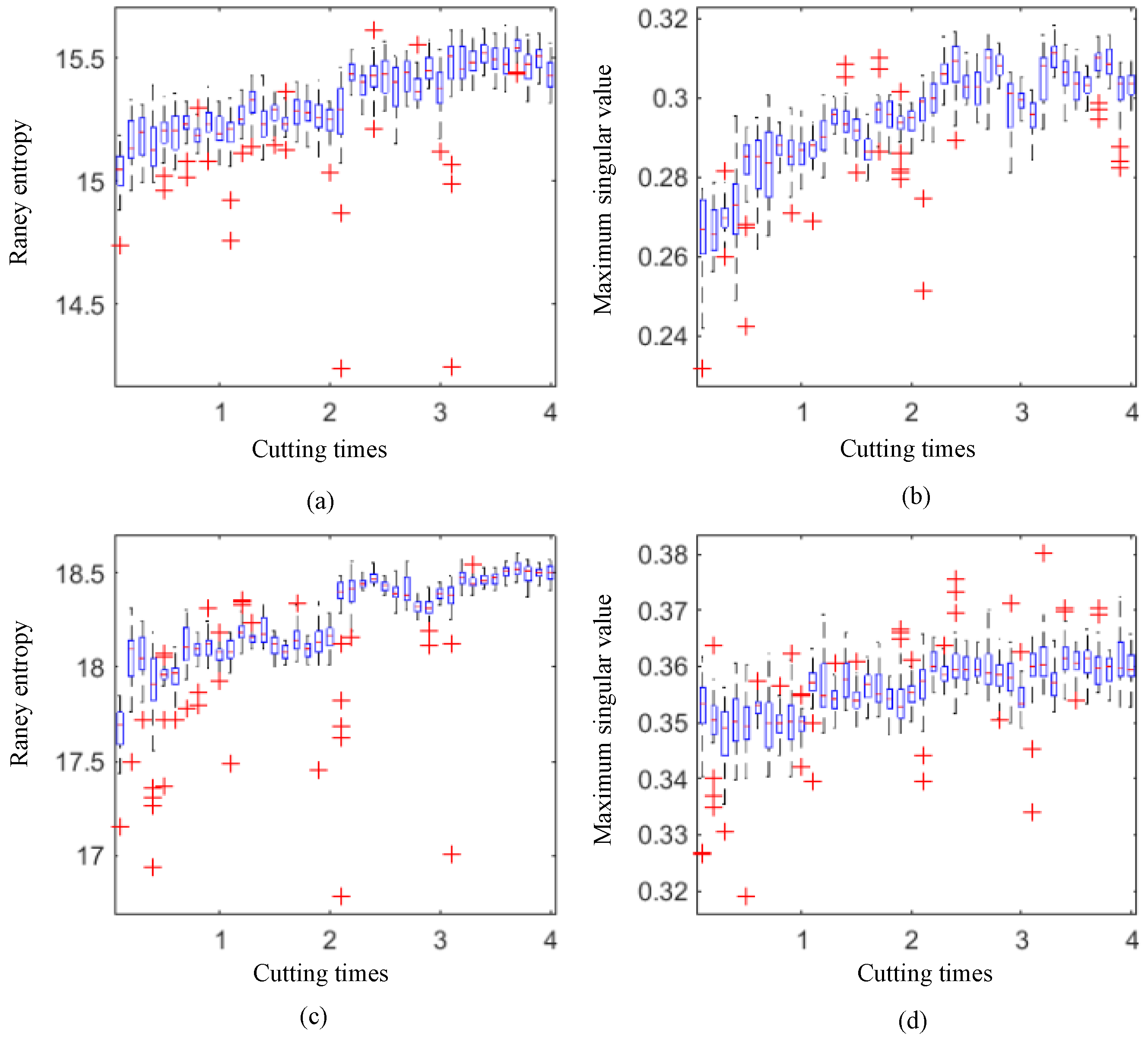
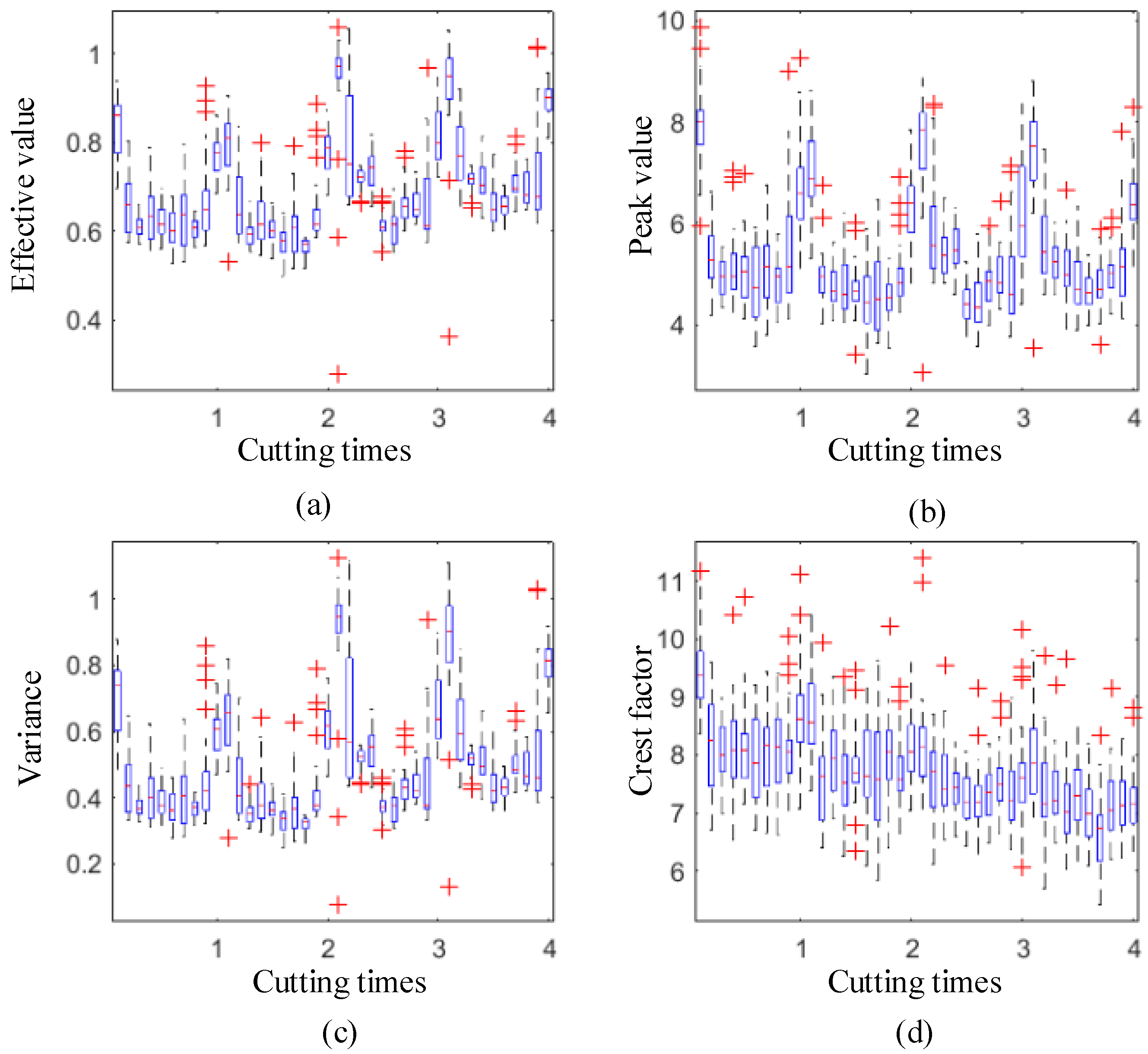
Figure 9 shows the variation law of the four features with the highest LER6 scores in Table 9 with the cutting process, in which Figure 9a is the Raney entropy of the time-frequency image of the fifth layer component after wavelet decomposition and Figure 9b is the original the maximum singular value of the normalized time–frequency image of the waveform. Figure 9c is the Raney entropy of the time–frequency image of the first layer component after wavelet decomposition, and Figure 9d is the normalization of the second layer component after wavelet decomposition. The maximum singular value of the time–frequency image shows that these four features are all dimensionless features. It can be seen that the above features all have good monotonicity and small fluctuation, and the change trend of feature 1 and feature 2 is the closest to the change trend of tool wear.

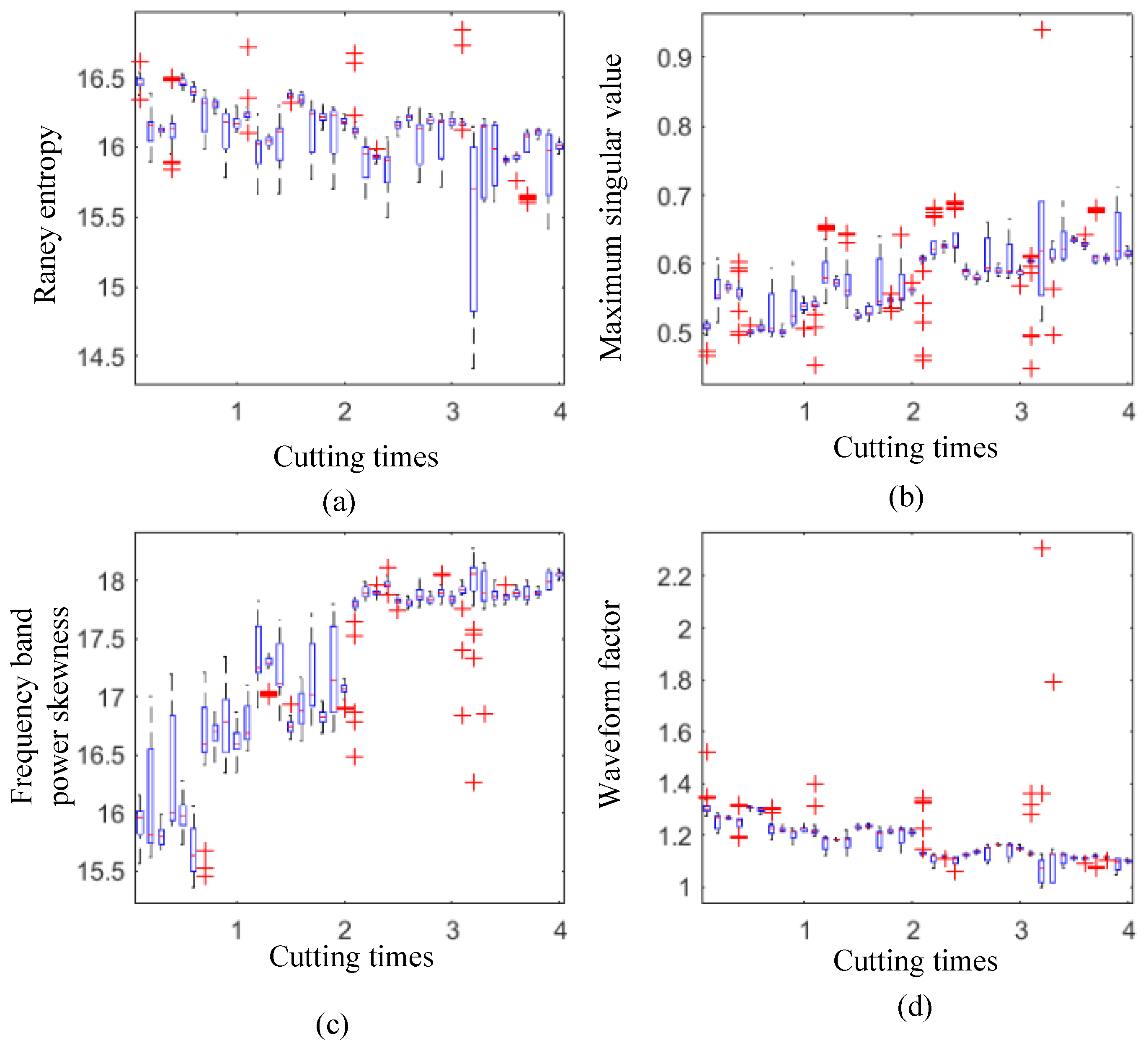
Figure 10, Figure 11 and Figure 12 are the variation laws of force signal characteristics, vibration signal characteristics and traditional characteristics of acoustic emission with cutting respectively. Compared with the variation law of acoustic emission time–frequency characteristics with cutting in Figure 9, these figures show that the method of feature extraction and selection proposed in this paper is effective.

4.3. Clustering Results and Tool Wear Status Identification

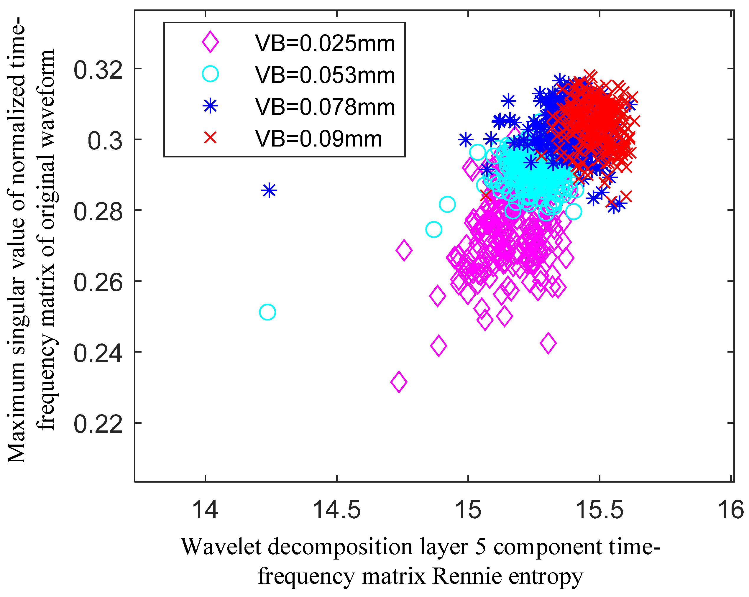
In order to realize the continuous monitoring of tool wear on the whole path in corner milling, the optimal feature set of acoustic emission obtained in this paper must be used. Below, the clustering sample set is constructed using the first two features in Table 9 to illustrate the clustering process. The sample distribution is shown in Figure 13.

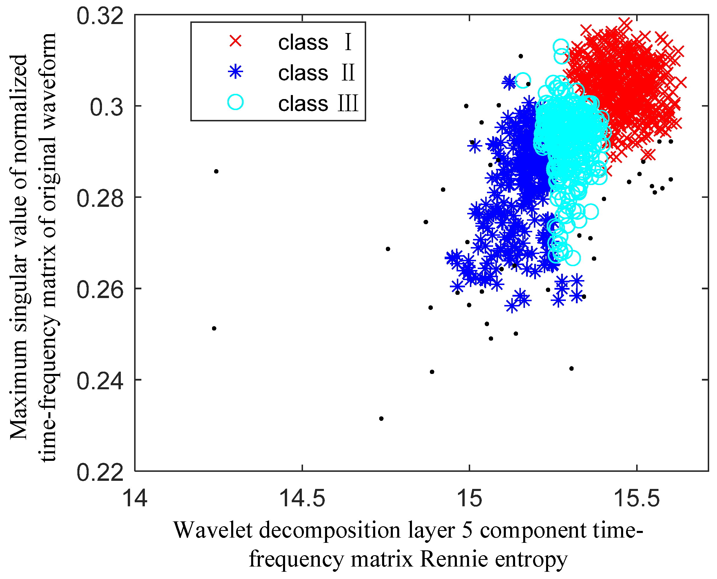
There are 1201 samples in the sample set, including 301 samples of class 1 (VB = 0.025 mm), 302 samples of class 2 (VB = 0.053 mm), 299 samples of class 3 (VB = 0.078 mm) and 299 samples of class 4 (VB = 0.09 mm). The sample set was input into CAGS, and the clustering result was obtained as shown in Figure 14.

As can be seen from Figure 13 and Figure 14, the algorithm basically identifies the first and second types of samples, but for the third and fourth types of samples, because the sample points are highly mixed, the algorithm can only identify the two classes as one class. In addition, in the initial clustering results, the algorithm marked the first class in the real label as class II, the second class in the real label as class III, and the first class in the real label as class III. Classes III and IV are marked as Class I. However, this problem can be successfully solved by the density factor $War$ proposed in Section 2.5.

As shown in

Table 10. Tool wear state assessment results based on $War$.

Real Label	VB (mm)	$\mathit{V}{\mathit{B}}_{\mathit{m}\mathit{a}\mathit{x}} \left(\mathbf{mm}\right)$	Label Clustering	$\mathit{W}\mathit{a}\mathit{r}$
1	0.025	0.18	II	0
2	0.053	0.24	III	0.59
3	0.078	0.26	I	0.80
4	0.09	0.27	I	0.80

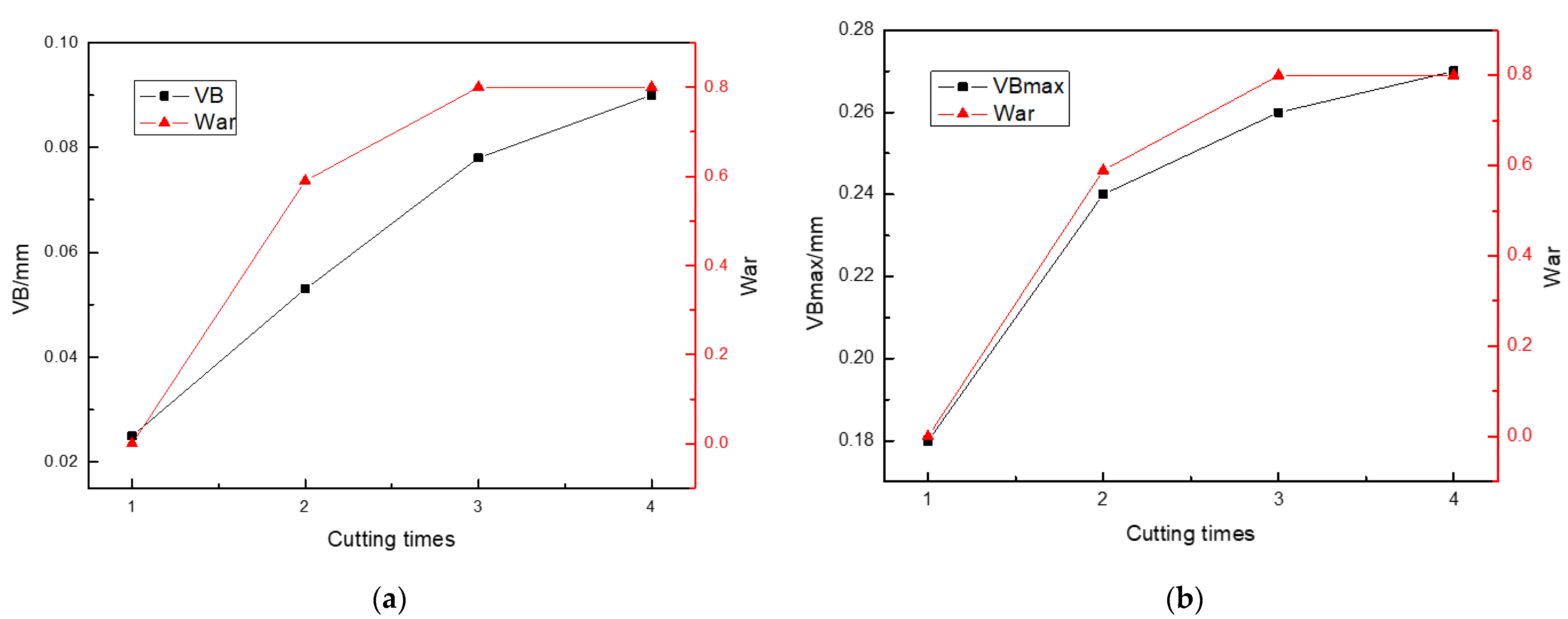
, although the cluster tag and the real tag cannot be matched, the density factor $War$ corresponding to the cluster tag can effectively match the tool wear value corresponding to the real tag, and the density factor gradually increases as the wear value increases. In order to more intuitively represent the effectiveness of $War$ for estimating wear value, (a) and (b) in Figure 15 give the double-coordinate curves of VB to $War$ and $V{B}_{max}$ to War, respectively. From the figure, it can be seen that the density factor can effectively estimate the changing trend of tool wear.

Finally, this paper verifies the effectiveness of the CAGS clustering results by comparing the identification accuracy with the currently popular classification algorithms, including the BP neural network, Bayesian network and SVM. BP neural network uses feedforward network, randomly selecting 150 samples of 4 different wear state samples as training data and setting 2 hidden layers and 10 neurons in each layer. The Bayesian network chose a minimum error rate-based method and evenly divided all samples corresponding to each wear state into four samples, forming four training datasets for cross-training. The SVM uses the radial basis kernel function, and the training data are the same as in the Bayesian network. The proposed recognition accuracy evaluation indexes are calculated respectively, and the comparison results are shown in

Table 11. Comparison of the wear identification accuracy of the peripheral corner milling tool. (The highest score of each index is marked in bold, and the lowest score is marked in italics).

Recognition Algorithm	PUR	CSM	NMI	CluCE	ClaCE
CAGS	0.58	0.64	0.43	0.61	0.45
BP network	0.70	0.71	0.48	0.53	0.52
Bayesian network	0.51	0.54	0.30	0.75	0.43
SVM	0.48	0.47	0.21	0.80	0.62

.

We can see that the BP neural network outperforms other methods in PUR, CSM, NMI, and CluCE, while the Bayesian network provides the best results considering ClaCE. However, the CAGS performs better than others on all the indexes, and compared with those supervised methods, the CAGS does not rely on extensive experiments to obtain the training data.

5. Conclusions

In this paper, clustering online monitoring based on the time–frequency intrinsic characteristics of acoustic emission and cluster density factor is proposed that realizes the unsupervised online monitoring of tool wear in corner milling. The results show that the cluster density factor could effectively characterize the real tool wear values. The following conclusions can be summarized:

(1)

In order to study and analyze the complexity of the corner milling of aviation structural parts and its influence on multi-sensor signals, a metal cutting condition monitoring platform based on multi-sensor information synchronous acquisition is built. A verification experiment of tool wear condition monitoring for corner peripheral milling is designed.

(2)

A method of tool wear-sensitive feature extraction based on the inherent features of time–frequency images is proposed. Unsupervised feature selection based on trend item analysis are used to obtain the best feature set. The effectiveness of the extracted sensitive features is verified.

(3)

The evolution law of sensitive characteristics with tool wear is analyzed. A tool wear monitoring method using the CAGS-based density factor is proposed. Compared with the supervised algorithms, the results show that the unsupervised monitoring system proposed in this paper has considerable recognition accuracy. However, in terms of robustness, our method has incomparable advantages over the supervised monitoring algorithms.

In brief, the unsupervised method based on CAGS is an effective solution for tool wear monitoring in the corner-milling process. However, the recognition accuracy and the robustness of the monitoring system need to be improved in further studies.