
Two-Stage Multi-Scale Fault Diagnosis Method for Rolling Bearings with Imbalanced Data

Abstract
:1. Introduction
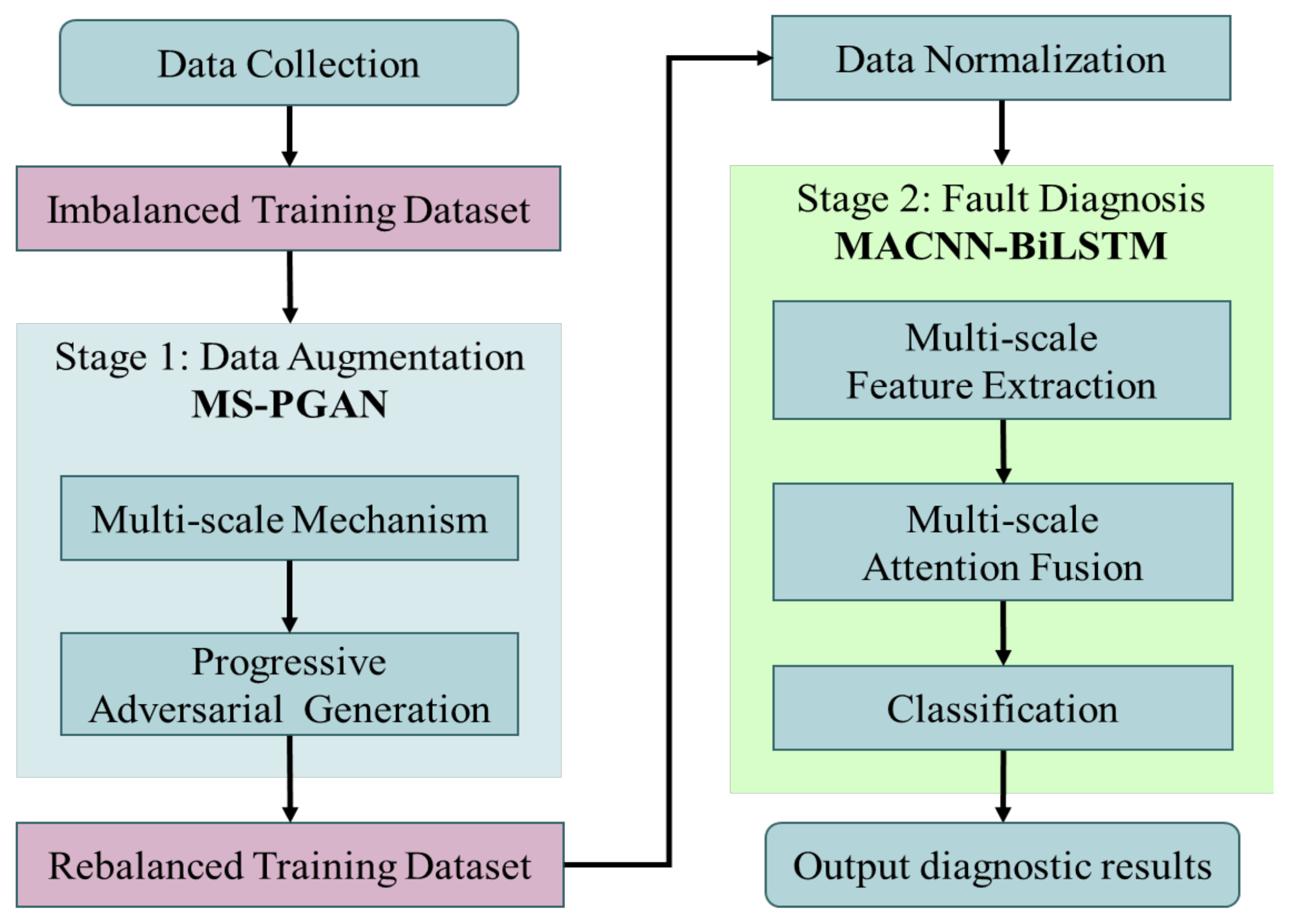
- Stage 1: A multiscale progressive generative adversarial network is proposed, to generate high-quality multi-scale data to rebalance the imbalanced datasets.
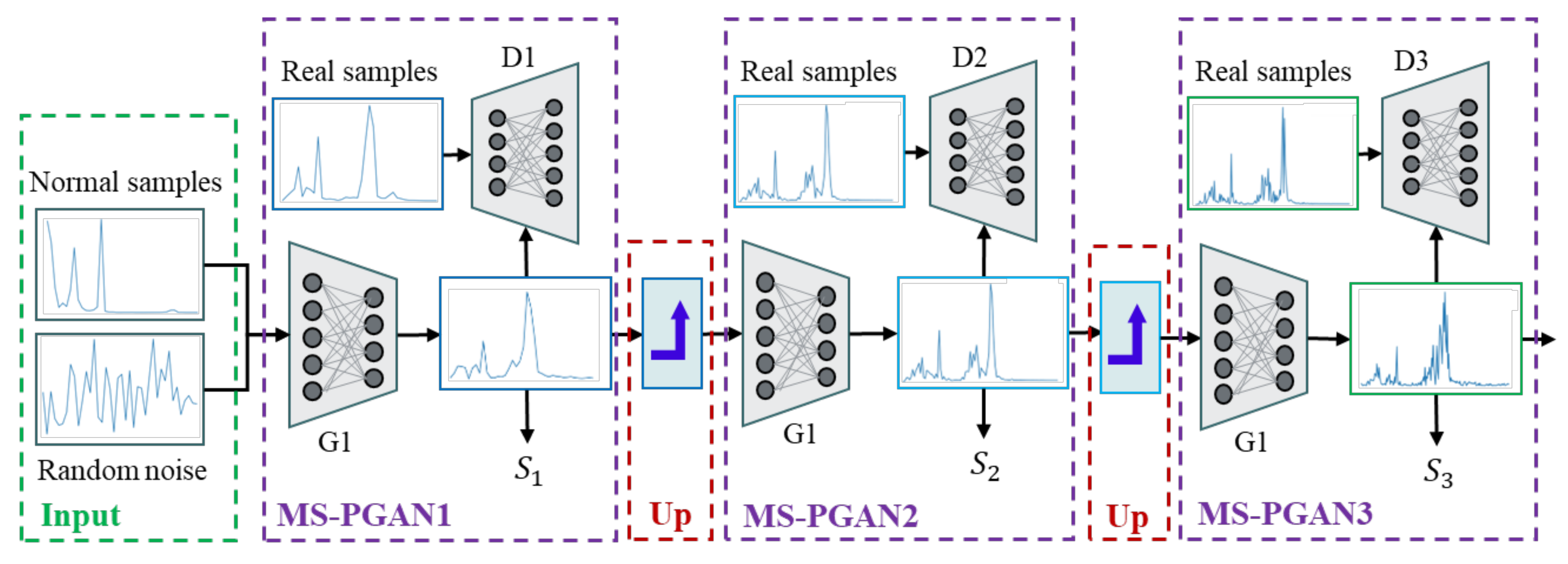
- A multi-scale GAN network structure with progressive growth has strong stability, which avoids the common problem of training failure in the GAN.
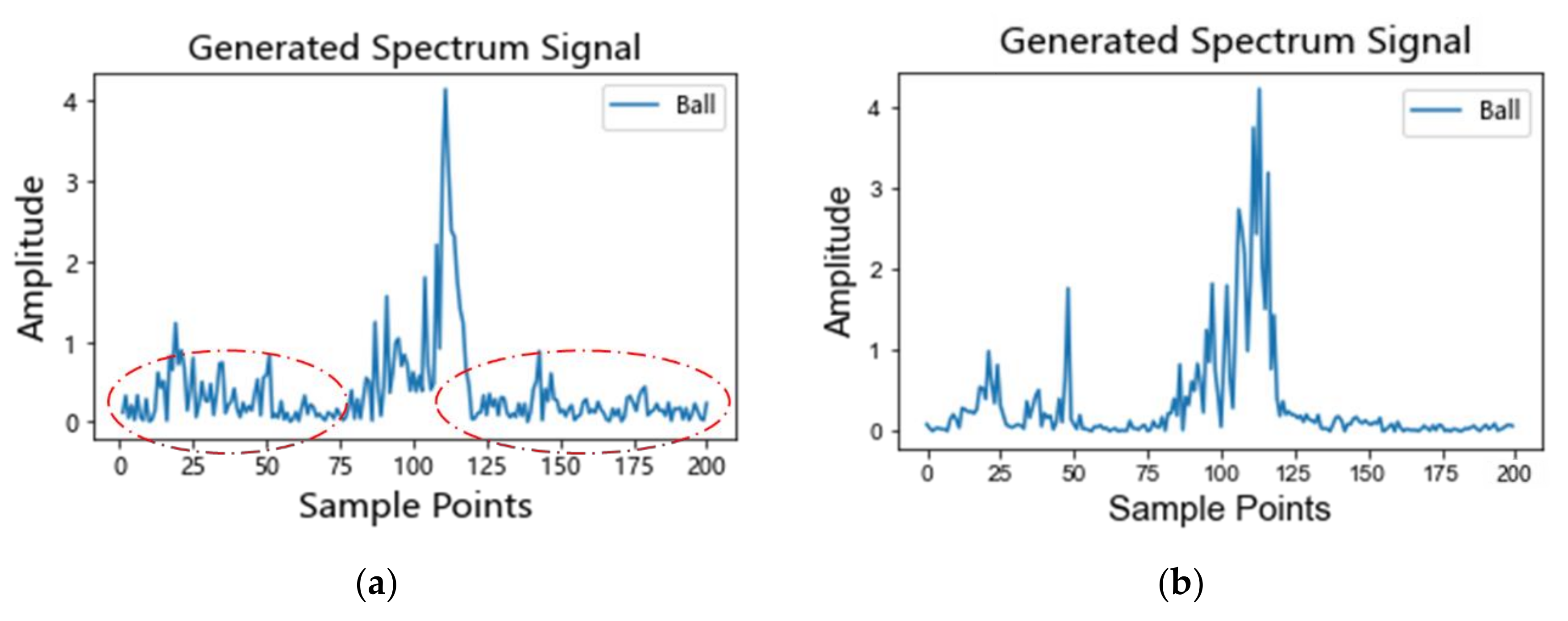
- The improved loss function MMD-WGP makes the generator model learn the distribution of fault samples from normal samples by introducing the transfer learning mechanism [37], which effectively improves the problem of random spectral noise and mode collapse.
- The local noise interpolation upsampling uses adaptive noise interpolation in the process of dimension promotion to protect the frequency information of the fault feature.
- Stage 2: Combined with multi-scale MS-PGAN, a diagnostic method based on a multi-scale attention fusion mechanism, named MACNN-BiLSTM, is proposed.
- The feature extraction structure of the proposed diagnosis method can combine the local feature extraction capability of the CNN and the global timing feature extraction capability of BiLSTM.
- The multi-scale attention fusion mechanism enables the model to fuse feature information extracted from different scales, which significantly improves the diagnostic capability of the model.
2. Theoretical Background
2.1. Convolutional Neural Network (CNN)
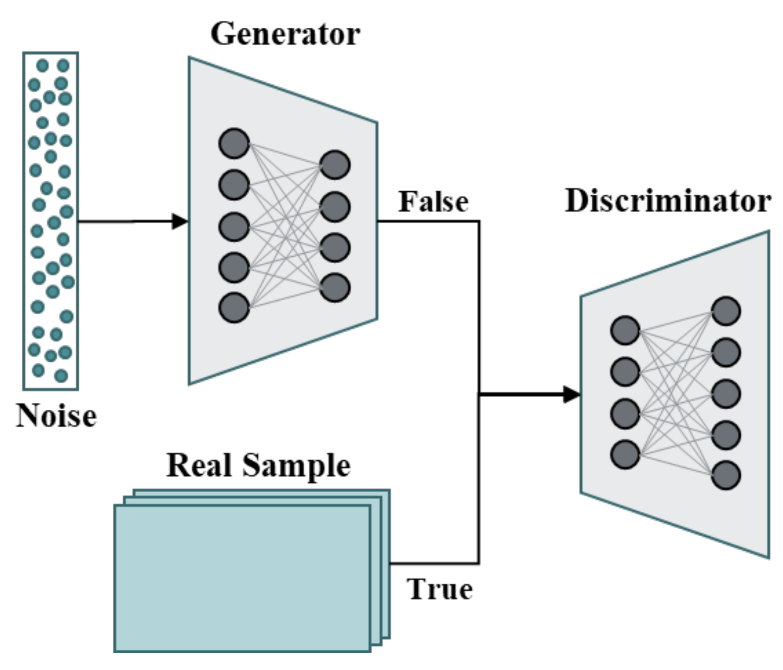
2.2. Generative Adversarial Network (GAN)
3. Proposed Methodology
3.1. MS-PGAN
3.1.1. The Structure of MS-PGAN
| Algorithm 1. The procedure of MS-PGAN |
| Input: |
| Output: |
| 1: for = 1 to 3 do 2: is 40: 3: 4: Satisfy Nash equilibrium do 5: 6: 7: end while 8: end if 9: is 100 or 200: 10: 11: , 12: Satisfy Nash equilibrium do 13: 14: 15: end while 16: end if |
| 17: end for |
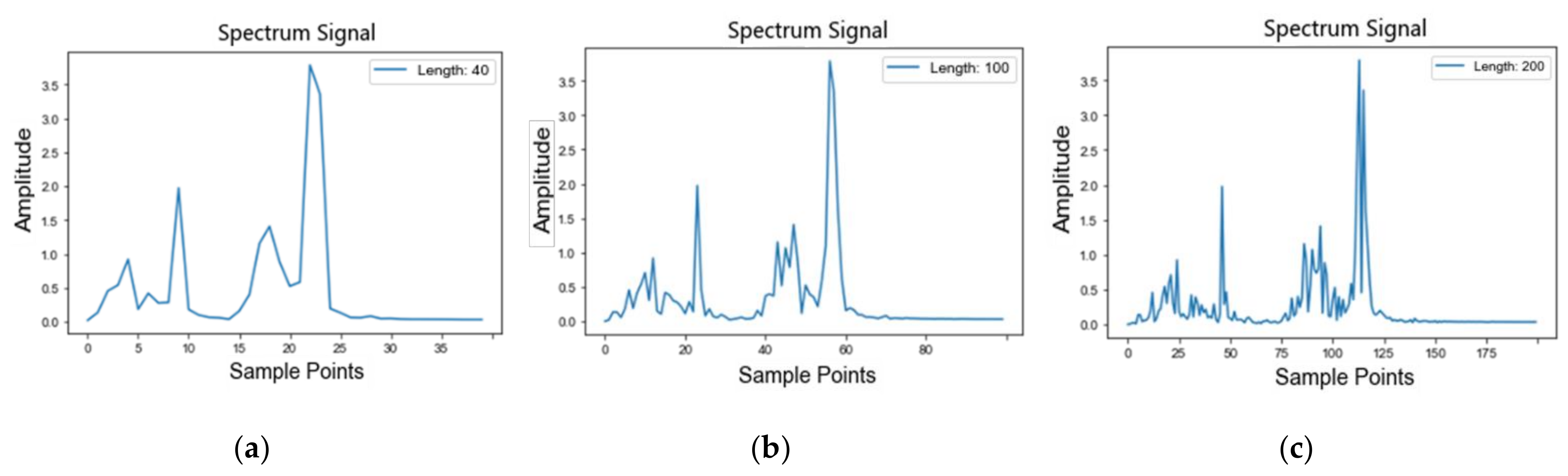
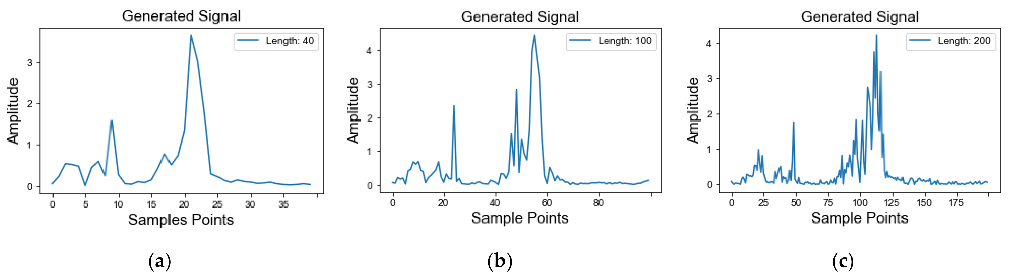
3.1.2. Multi-Scale Mechanism
- Low-dimensional rough scale: if is 200 and is 5 and the resolution is 40-length, which mainly includes the features of spectral peak.
- Middle-dimensional scale: if is 200, is 2 and the resolution is 100-length, so more harmonic features are added.
- High dimensional scale: if is 200, is 1 and the resolution is 200-length; this enriches the detailed features of the signal, including the complete frequency domain information.
3.1.3. Improved GAN Loss Function with Transfer Learning
3.1.4. Local Noise Interpolation Upsampling
3.2. MS-PGAN Combining MACNN-BiLSTM
| Algorithm 2. The procedure of MACNN-BiLSTM |
| Input: |
| Output: |
| 1: while not converge do 2: for all do 3: 4: for = 1 to 3 do 5: 6: end for 7: MP(LeakyReLU( 8: Attention(BiLSTM( 9: GMP( 10: end for 11: Softmax(FC(Concat() 12: Concat ( 13: Softmax(FC( 14: end while |
4. Experimental Study
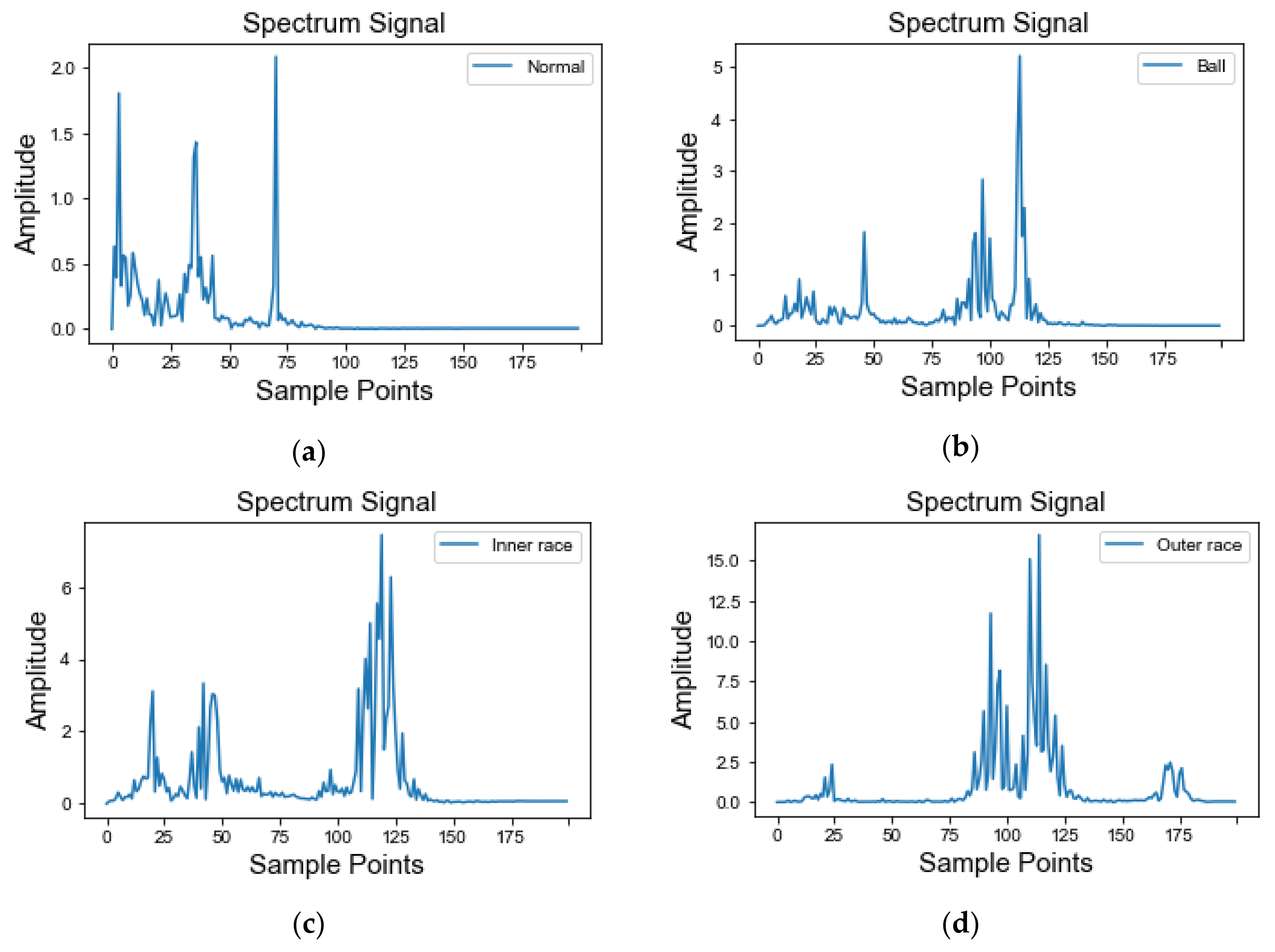
4.1. Dataset Descriptions and Preprocessing
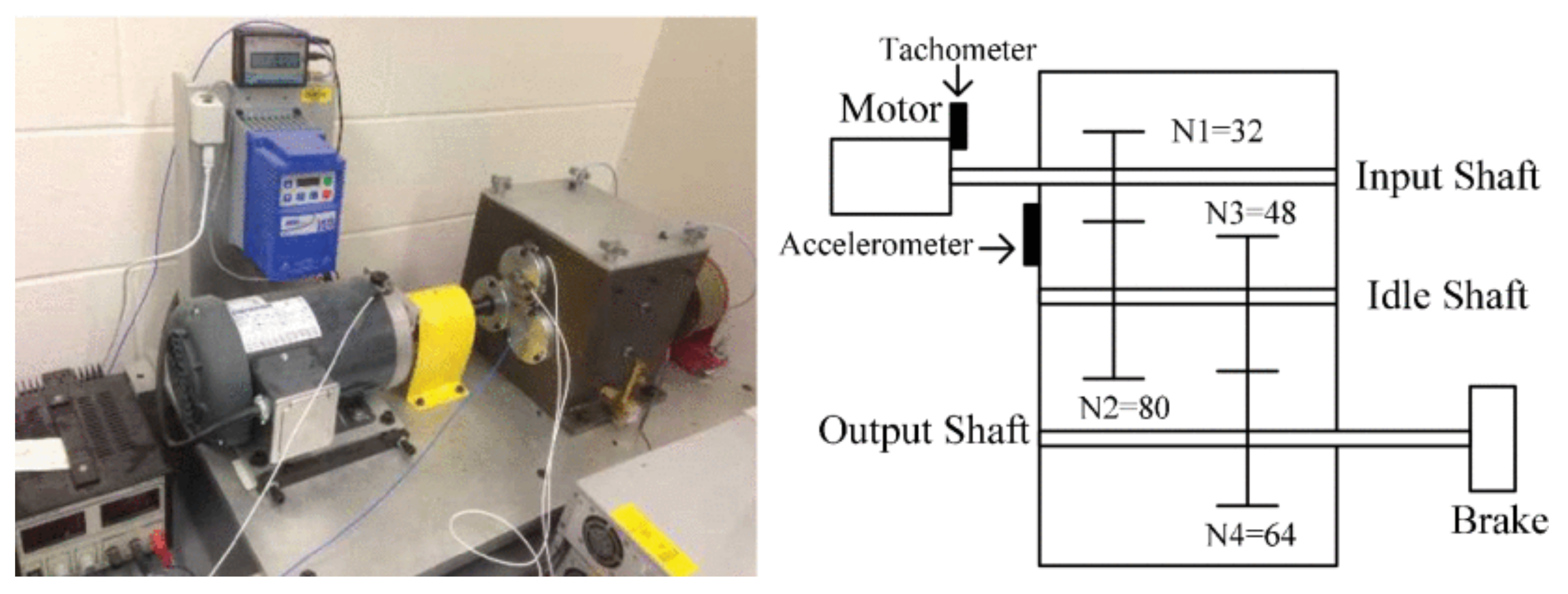
4.1.1. Case 1: UConn Dataset
4.1.2. Case 2: CWRU Dataset
4.1.3. Data Preprocessing
4.2. Stage 1: Data Augmentation
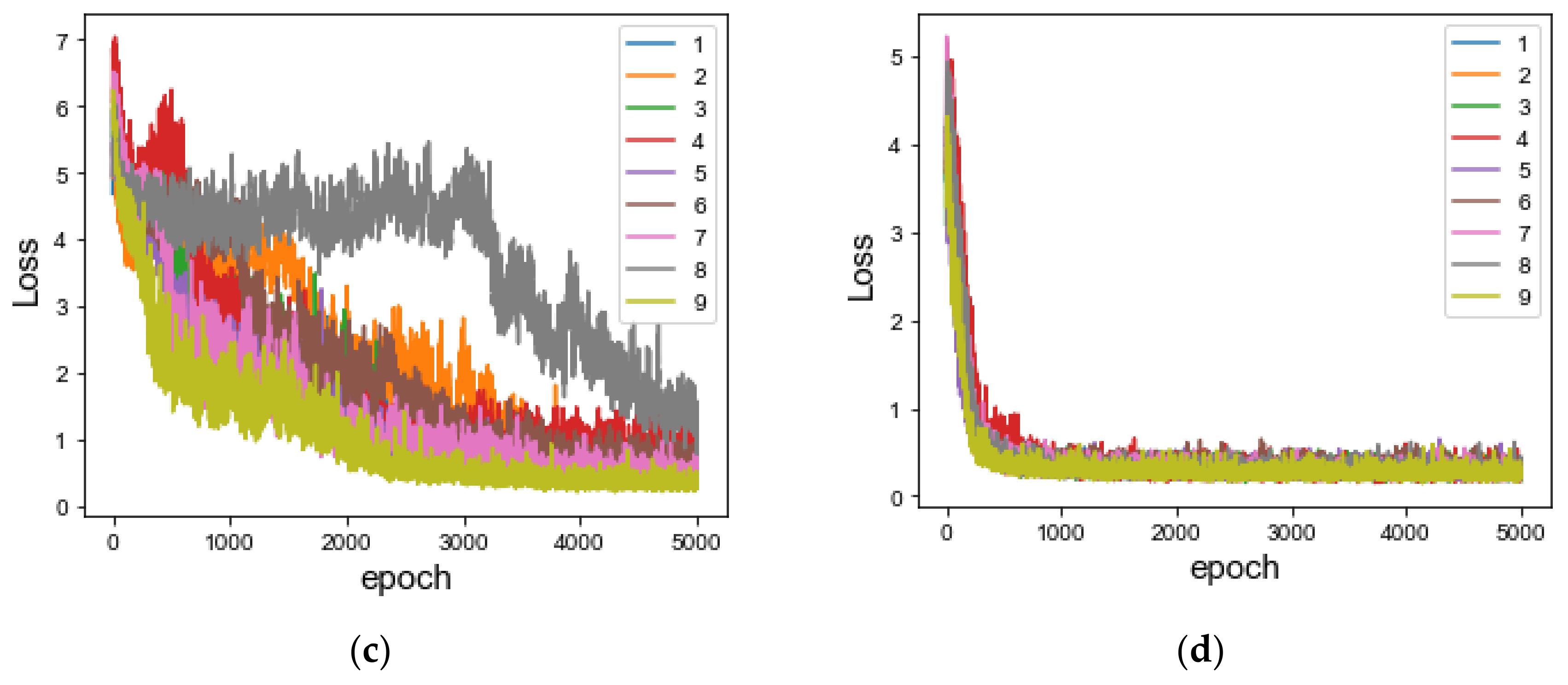
4.2.1. Experiments Results of Data Augmentation
4.2.2. Performance Analysis
4.3. Stage 2: Fault Diagnosis
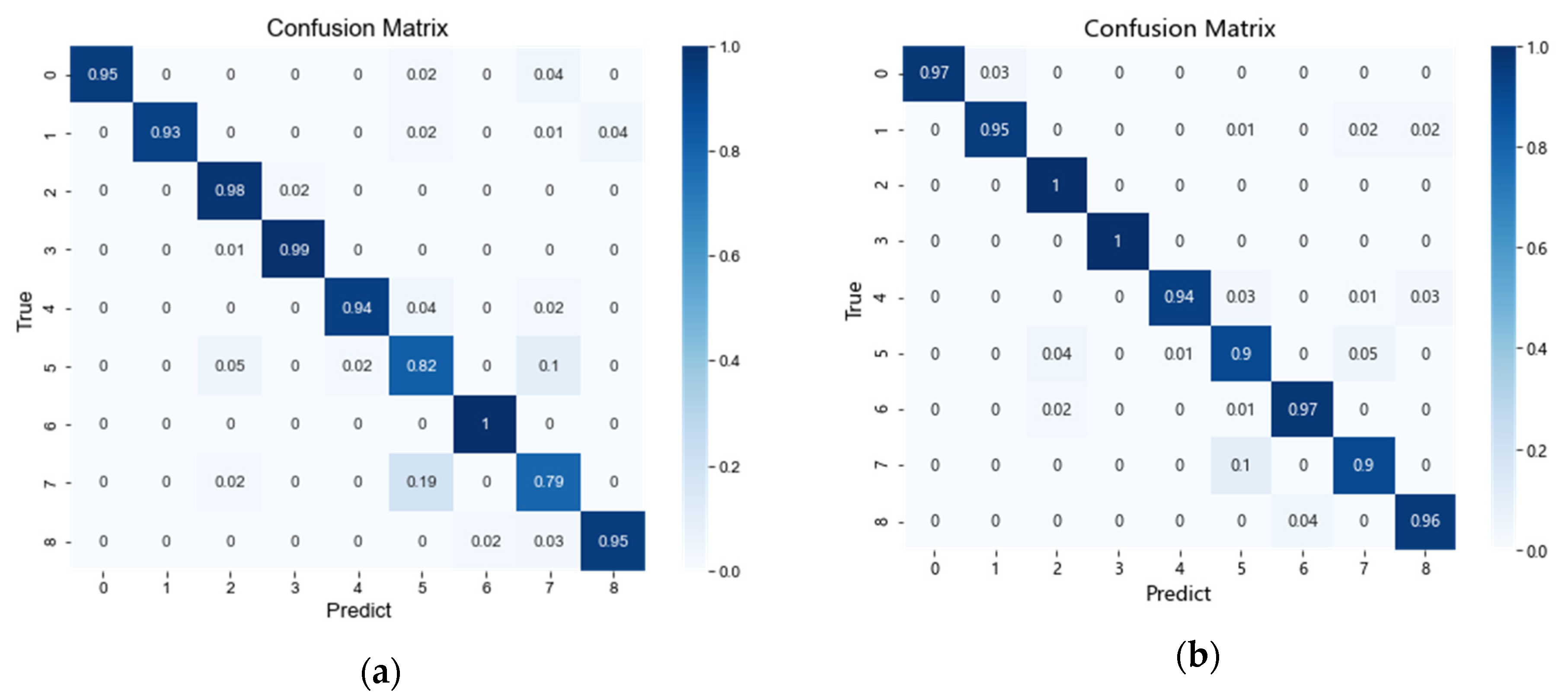
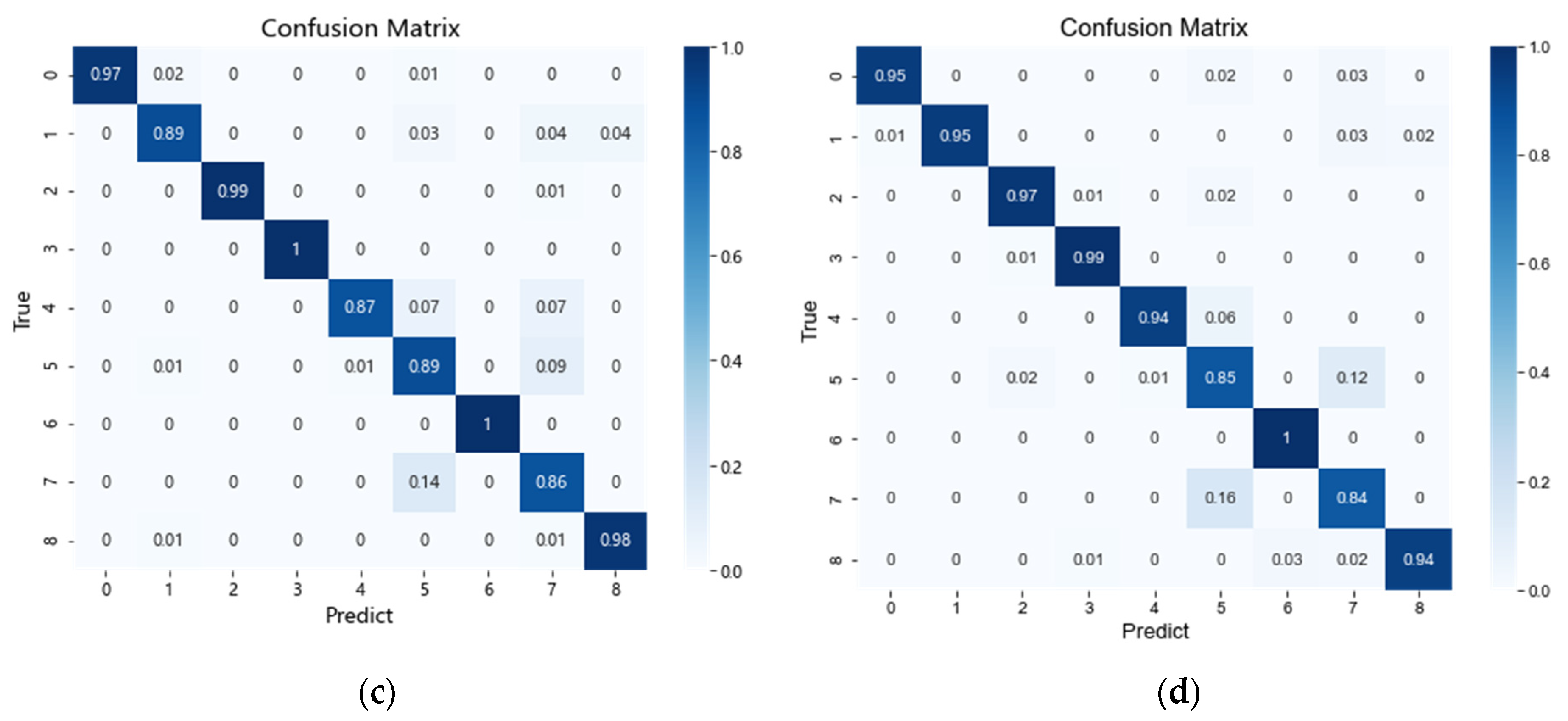
4.3.1. Experimental Results of Data Augmentation
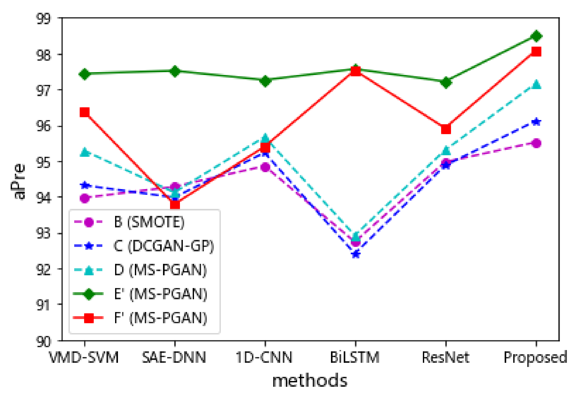
4.3.2. Performance Analysis
5. Conclusions
Author Contributions
Funding
Institutional Review Board Statement
Informed Consent Statement
Data Availability Statement
Conflicts of Interest
Abbreviations
| 1D-CNN | One-dimensional Convolutional Neural Network |
| 1D-Conv | One-dimensional Convolution Layer |
| 1D-ConvT | One-dimensional Transposed Convolution Layer |
| BiLSTM | Bidirectional Long Short-Term Memory Network |
| CNN | Convolutional Neural Network |
| DNN | Deep Neural Network |
| DCGAN | Deep Convolutional Generative Adversarial Network |
| IMF | Intrinsic Mode Function |
| GAN | Generative Adversarial Network |
| LSTM | Long Short-Term Memory Network |
| MS-PGAN | Multi-scale Progressive Generative Adversarial Network |
| MACNN-BiLSTM | Multi-scale Attention CNN-BiLSTM |
| MMD | Maximum Mean Discrepancy |
| ResNet | Deep Residual Network |
| ReLU | Rectified Linear Units |
| SAE | Stack Auto Encoder |
| SVM | Support Vector Machine |
| Tanh | Hyperbolic Tangent |
| VMD | Variational Mode Decomposition |
References
- Hoang, D.T.; Kang, H.J. A survey on deep learning based bearing fault diagnosis. Neurocomputing 2019, 335, 327–335. [Google Scholar] [CrossRef]
- Cerrada, M.; Sánchez, R.V.; Li, C.; Pacheco, F.; Cabrera, D.; de Oliveira, J.V.; Vásquez, R.E. A review on data-driven fault severity assessment in rolling bearings. Mech. Syst. Signal Process. 2018, 99, 169–196. [Google Scholar] [CrossRef]
- Lei, Y.; Lin, J.; He, Z.; Zuo, M.J. A review on empirical mode decomposition in fault diagnosis of rotating machinery. Mech. Syst. Signal Process. 2013, 35, 108–126. [Google Scholar] [CrossRef]
- Xia, M.; Li, T.; Xu, L.; Liu, L.; De Silva, C.W. Fault diagnosis for rotating machinery using multiple sensors and convolutional neural networks. IEEE/ASME Trans. Mechatron. 2017, 23, 101–110. [Google Scholar] [CrossRef]
- Lei, Y.; Jia, F.; Zhou, X. Health monitoring method of mechanical equipment with big data based on deep learning theory. Chin. J. Mech. Eng. 2015, 51, 49–56. [Google Scholar] [CrossRef]
- Zhou, Q.; Shen, H.; Zhao, J. Review and prospect of mechanical equipment health management based on deep learning. Mod. Mach. 2018, 4, 19–27. [Google Scholar]
- Islam, M.M.; Kim, J.M. Automated bearing fault diagnosis scheme using 2D representation of wavelet packet transform and deep convolutional neural network. Comput. Ind. 2019, 106, 142–153. [Google Scholar] [CrossRef]
- Tang, X.; Hu, B.; Wen, H. Fault Diagnosis of Hydraulic Generator Bearing by VMD-Based Feature Extraction and Classification. Iran. J. Sci. Technol. Trans. Electr. Eng. 2021, 45, 1227–1237. [Google Scholar] [CrossRef]
- Lei, Y. Intelligent Fault Diagnosis and Remaining Useful Life Prediction of Rotating Machinery; Butterworth-Heinemann Elsevier Ltd.: Oxford, UK, 2016. [Google Scholar]
- Eren, L.; Ince, T.; Kiranyaz, S. A generic intelligent bearing fault diagnosis system using compact adaptive 1D CNN classifier. J. Signal Process. Syst. 2019, 91, 179–189. [Google Scholar] [CrossRef]
- Rhanoui, M.; Mikram, M.; Yousfi, S.; Barzali, S. A CNN-BiLSTM model for document-level sentiment analysis. Mach. Learn. Knowl. Extr. 2019, 1, 832–847. [Google Scholar] [CrossRef] [Green Version]
- Duan, J.; Shi, T.; Zhou, H.; Xuan, J.; Wang, S. A novel ResNet-based model structure and its applications in machine health monitoring. J. Vib. Control 2021, 27, 1036–1050. [Google Scholar] [CrossRef]
- Hochreiter, S.; Schmidhuber, J. Long short-term memory. Neural Comput. 1997, 9, 1735–1780. [Google Scholar] [CrossRef] [PubMed]
- Huang, T.; Zhang, Q.; Tang, X.; Zhao, S.; Lu, X. A novel fault diagnosis method based on CNN and LSTM and its application in fault diagnosis for complex systems. Artif. Intell. Rev. 2022, 55, 1289–1315. [Google Scholar] [CrossRef]
- Jiao, Y.; Wei, Y.; An, D.; Li, W.; Wei, Q. An Improved CNN-LSTM Network Based on Hierarchical Attention Mechanism for Motor Bearing Fault Diagnosis. Res. Square 2021. [Google Scholar] [CrossRef]
- Cheng, F.; Cai, W.; Zhang, X.; Liao, H.; Cui, C. Fault detection and diagnosis for Air Handling Unit based on multiscale convolutional neural networks. Energy Build. 2021, 236, 110795. [Google Scholar] [CrossRef]
- Zareapoor, M.; Shamsolmoali, P.; Yang, J. Oversampling adversarial network for class-imbalanced fault diagnosis. Mech. Syst. Signal Process. 2021, 149, 107175. [Google Scholar] [CrossRef]
- Chawla, N.V.; Bowyer, K.W.; Hall, L.O.; Kegelmeyer, W.P. SMOTE: Synthetic minority over-sampling technique. J. Artif. Intell. Res. 2002, 16, 321–357. [Google Scholar] [CrossRef]
- Shi, H.; Chen, Y.; Chen, X. Summary of research on SMOTE oversampling and its improved algorithms. CAAI Trans. Intell. Syst. 2019, 14, 1073–1083. [Google Scholar]
- Goodfellow, I.; Pouget-Abadie, J.; Mirza, M.; Xu, B.; Warde-Farley, D.; Ozair, S.; Bengio, Y. Generative adversarial nets. Adv. Neural Inf. Process. Syst. 2014, 27. [Google Scholar] [CrossRef]
- Hong, Y.; Hwang, U.; Yoo, J.; Yoon, S. How generative adversarial networks and their variants work: An overview. ACM Comput. Surv. (CSUR) 2019, 52, 1–43. [Google Scholar] [CrossRef] [Green Version]
- Sun, J.; Zhong, G.; Chen, Y.; Liu, Y.; Li, T.; Huang, K. Generative adversarial networks with mixture of t-distributions noise for diverse image generation. Neural Netw. 2020, 122, 374–381. [Google Scholar] [CrossRef] [PubMed]
- Zheng, Y.J.; Zhou, X.H.; Sheng, W.G.; Xue, Y.; Chen, S.Y. Generative adversarial network based telecom fraud detection at the receiving bank. Neural Netw. 2018, 102, 78–86. [Google Scholar] [CrossRef] [PubMed]
- Lu, Q.; Tao, Q.; Zhao, Y.; Liu, M. Sketch simplification based on conditional random field and least squares generative adversarial networks. Neurocomputing 2018, 316, 178–189. [Google Scholar] [CrossRef]
- Gao, X.; Deng, F.; Yue, X. Data augmentation in fault diagnosis based on the Wasserstein generative adversarial network with gradient penalty. Neurocomputing 2020, 396, 487–494. [Google Scholar] [CrossRef]
- Lee, Y.O.; Jo, J.; Hwang, J. Application of deep neural network and generative adversarial network to industrial maintenance: A case study of induction motor fault detection. In Proceedings of the 2017 IEEE International Conference on Big Data (Big Data), Boston, MA, USA, 11–14 December 2017; pp. 3248–3253. [Google Scholar]
- Radford, A.; Metz, L.; Chintala, S. Unsupervised Representation Learning with Deep Convolutional Generative Adversarial Networks. arXiv 2016, arXiv:11511.06434. [Google Scholar]
- Arjovsky, M.; Chintala, S.; Bottou, L. Wasserstein GAN. arXiv, 2017; arXiv:11701.07875. [Google Scholar]
- Gulrajani, I.; Ahmed, F.; Arjovsky, M.; Dumoulin, V.; Courville, A.C. Improved training of wasserstein gans. Adv. Neural Inf. Processing Syst. 2017, 30, 5769–5779. [Google Scholar] [CrossRef]
- Shao, S.; Wang, P.; Yan, R. Generative adversarial networks for data augmentation in machine fault diagnosis. Comput. Ind. 2019, 106, 85–93. [Google Scholar] [CrossRef]
- Zhang, A.; Su, L.; Zhang, Y.; Fu, Y.; Wu, L.; Liang, S. EEG data augmentation for emotion recognition with a multiple generator conditional Wasserstein GAN. Complex Intell. Syst. 2021, 1–13. [Google Scholar] [CrossRef]
- Li, Z.; Zheng, T.; Wang, Y.; Cao, Z.; Guo, Z.; Fu, H. A novel method for imbalanced fault diagnosis of rotating machinery based on generative adversarial networks. IEEE Trans. Instrum. Meas. 2020, 70, 1–17. [Google Scholar] [CrossRef]
- Zhou, F.; Yang, S.; Fujita, H.; Chen, D.; Wen, C. Deep learning fault diagnosis method based on global optimization GAN for unbalanced data. Knowl.-Based Syst. 2020, 187, 104837. [Google Scholar] [CrossRef]
- Zhang, W.; Li, X.; Jia, X.D.; Ma, H.; Luo, Z.; Li, X. Machinery fault diagnosis with imbalanced data using deep generative adversarial networks. Measurement 2020, 152, 107377. [Google Scholar] [CrossRef]
- Zhang, H.; Xu, T.; Li, H.; Zhang, S.; Wang, X.; Huang, X.; Metaxas, D.N. Stackgan: Text to photo-realistic image synthesis with stacked generative adversarial networks. In Proceedings of the IEEE International Conference on Computer Vision, Venice, Italy, 22–29 October 2017; pp. 5907–5915. [Google Scholar]
- Karras, T.; Aila, T.; Laine, S.; Lehtinen, J. Progressive growing of gans for improved quality, stability, and variation. arXiv 2017, arXiv:1710.10196. [Google Scholar]
- Pan, S.J.; Yang, Q. A survey on transfer learning. IEEE Trans. Knowl. Data Eng. 2009, 22, 1345–1359. [Google Scholar] [CrossRef]
- Shrestha, A.; Mahmood, A. Review of deep learning algorithms and architectures. IEEE Access 2019, 7, 53040–53065. [Google Scholar] [CrossRef]
- Ratliff, L.J.; Burden, S.A.; Sastry, S.S. On the characterization of local Nash equilibria in continuous games. IEEE Trans. Autom. Control 2016, 61, 2301–2307. [Google Scholar] [CrossRef] [Green Version]
- Gretton, A.; Borgwardt, K.M.; Rasch, M.J.; Schölkopf, B.; Smola, A. A kernel two-sample test. J. Mach. Learn. Res. 2012, 13, 723–773. [Google Scholar]
- Yang, B.; Xu, S.; Lei, Y.; Lee, C.G.; Stewart, E.; Roberts, C. Multi-source transfer learning network to complement knowledge for intelligent diagnosis of machines with unseen faults. Mech. Syst. Signal Process. 2022, 162, 108095. [Google Scholar] [CrossRef]
- Siarohin, A.; Sangineto, E.; Sebe, N. Whitening and Coloring Batch Transform for GANs. In Proceedings of the Seventh International Conference on Learning Representations, New Orleans, LA, USA, 6–9 May 2019. [Google Scholar]
- Cao, P.; Zhang, S.; Tang, J. Preprocessing-free gear fault diagnosis using small datasets with deep convolutional neural network-based transfer learning. IEEE Access 2018, 6, 26241–26253. [Google Scholar] [CrossRef]
- Welcome to the Case Western Reserve University Bearing Data Center Website. Available online: https://engineering.case.edu/bearingdatacenter/welcome (accessed on 1 May 2021).
- Singleton, R.K.; Strangas, E.G.; Aviyente, S. Time-frequency complexity based remaining useful life (RUL) estimation for bearing faults. In Proceedings of the 2013 9th IEEE International Symposium on Diagnostics for Electric Machines, Power Electronics and Drives (SDEMPED), Valencia, Spain, 27–30 August 2013; pp. 600–606. [Google Scholar]


| Layer | Input Size | Output Size | BN | Activation Function | Layer |
|---|---|---|---|---|---|
| 1D-ConvT 1D-ConvT | B,N,1,1 | B,64 * 2,1,5 | yes | ReLU | 1D-ConvT |
| B,64 * 2,1,5 | B,64 * 4,1,12 | yes | ReLU | 1D-ConvT | |
| 1D-ConvT 1D-ConvT | B,64 * 4,1,12 | B,64 * 2,1,24 | yes | ReLU | 1D-ConvT |
| B,64 * 2,1,24 | B,64,1,50 | yes | ReLU | 1D-ConvT | |
| 1D-ConvT | B,64,1,50 | B,1,1,N | yes | Tanh | 1D-ConvT |
| Layer | Input Size | Output Size | BN | Activation Function | Layer |
|---|---|---|---|---|---|
| 1D-Conv 1D-Conv | B,1,1,N | B,64,1,50 | yes | LeakyReLU | 1D-Conv |
| B,64,1,50 | B,64 * 2,1,24 | yes | LeakyReLU | 1D-Conv | |
| 1D-Conv 1D-Conv | B,64 * 2,1,24 | B,64 * 4,1,12 | yes | LeakyReLU | 1D-Conv |
| B,64 * 4,1,12 | B,64 * 2,1,5 | yes | LeakyReLU | 1D-Conv | |
| 1D-Conv | B,64 * 2,1,5 | B,1,1,1 | yes | Softmax | 1D-Conv |
| Layer | Input Size | Kernel Size | Stride | Padding |
|---|---|---|---|---|
| input | B,1, N | |||
| 1D-Conv Block1 | B,128,N | 5,1 | 1,1 | yes |
| 1D-Conv Block2 | B,128,N | 5,1 | 1,1 | yes |
| 1D-Conv Block3 | B,128,N | 5,1 | 1,1 | yes |
| ADD | B,128,N | |||
| LeakyReLU | B,128,N | |||
| Max Pool | B,128,N | 2,1 | 1,1 | yes |
| BiLSTM | B,128,N/2 | |||
| Attention | B,128,256 | |||
| GAP | B,4,256 | 4,1 | 1,1 | yes |
| MS-Attention | B,256,1 | |||
| FC | 96,Num | |||
| softmax | Num,Num |
| State | Location | A | B | C | D | T1 | B’ | C’ | D’ | T1’ |
|---|---|---|---|---|---|---|---|---|---|---|
| 0 | Normal | 312 | 312 | 312 | 312 | 104 | - | - | - | - |
| 1 | Missing Tooth | 32 | 32 + 280 | 32 + 280 | 32 + 280 | 104 | 280 | 280 | 280 | 104 |
| 2 | Root Crack | 32 | 32 + 280 | 32 + 280 | 32 + 280 | 104 | 280 | 280 | 280 | 104 |
| 3 | Spalling | 32 | 32 + 280 | 32 + 280 | 32 + 280 | 104 | 280 | 280 | 280 | 104 |
| 4 | Chipping 5a | 32 | 32 + 280 | 32 + 280 | 32 + 280 | 104 | 280 | 280 | 280 | 104 |
| 5 | Chipping 4a | 32 | 32 + 280 | 32 + 280 | 32 + 280 | 104 | 280 | 280 | 280 | 104 |
| 6 | Chipping 3a | 32 | 32 + 280 | 32 + 280 | 32 + 280 | 104 | 280 | 280 | 280 | 104 |
| 7 | Chipping 2a | 32 | 32 + 280 | 32 + 280 | 32 + 280 | 104 | 280 | 280 | 280 | 104 |
| 8 | Chipping 1a | 32 | 32 + 280 | 32 + 280 | 32 + 280 | 104 | 280 | 280 | 280 | 104 |
| State | Location | Degree (mm) | E | F | E’ | F’ | T2 |
|---|---|---|---|---|---|---|---|
| 0 | Normal | 0.000 | 840 | 840 | 840 | 840 | 360 |
| 1 | Ball | 0.1778 | 84 | 44 | 84 + 756 | 44 + 796 | 360 |
| 2 | Inner race | 0.1778 | 84 | 44 | 84 + 756 | 44 + 796 | 360 |
| 3 | Outer race | 0.1778 | 84 | 44 | 84 + 756 | 44 + 796 | 360 |
| 4 | Ball | 0.3556 | 84 | 44 | 84 + 756 | 44 + 796 | 360 |
| 5 | Inner race | 0.3556 | 84 | 44 | 84 + 756 | 44 + 796 | 360 |
| 6 | Outer race | 0.3556 | 84 | 44 | 84 + 756 | 44 + 796 | 360 |
| 7 | Ball | 0.5334 | 84 | 44 | 84 + 756 | 44 + 796 | 360 |
| 8 | Inner race | 0.5334 | 84 | 44 | 84 + 756 | 44 + 796 | 360 |
| 9 | Outer race | 0.5334 | 84 | 44 | 84 + 756 | 44 + 796 | 360 |
| Data Scale | Imbalance | Rebalance | ||||||
|---|---|---|---|---|---|---|---|---|
| Original | SMOTE | DCGAN-GP | MS-PGAN | |||||
| Dataset A | Dataset B | Dataset C | Dataset D | |||||
| aPre | aRec | aPre | aRec | aPre | aRec | aPre | aRec | |
| Low | 88.48 | 88.46 | 88.74 | 88.35 | 90.84 | 90.59 | 91.68 | 91.67 |
| Middle | 90.93 | 90.60 | 93.13 | 93.06 | 93.98 | 93.91 | 94.36 | 94.34 |
| High | 92.79 | 92.84 | 93.77 | 93.91 | 94.32 | 94.34 | 95.29 | 95.19 |
| Data Scale | Imbalance | Pure Generated Data | ||||||
|---|---|---|---|---|---|---|---|---|
| Original | SMOTE | DCGAN-GP | MS-PGAN | |||||
| Dataset A | Dataset B’ | Dataset C’ | Dataset D’ | |||||
| aPre | aRec | aPre | aRec | aPre | aRec | aPre | aRec | |
| Low | 88.48 | 88.46 | 87.91 | 87.14 | 88.74 | 88.35 | 90.73 | 90.50 |
| Middle | 90.93 | 90.60 | 92.37 | 92.31 | 93.58 | 93.15 | 94.18 | 93.99 |
| High | 92.79 | 92.84 | 93.65 | 93.63 | 94.12 | 94.06 | 94.80 | 94.71 |
| Methods | Imbalance | Balance | ||||||
|---|---|---|---|---|---|---|---|---|
| Dataset A | SMOTE | DCGAN-GP | MS-PGAN | |||||
| Dataset B | Dataset C | Dataset D | ||||||
| aPre | aRec | aPre | aRec | aPre | aRec | aPre | aRec | |
| VMD-SVM | 92.79 | 92.84 | 93.97 | 93.91 | 94.32 | 94.34 | 95.29 | 95.19 |
| SAE-DNN | 93.38 | 93.18 | 94.28 | 94.12 | 93.98 | 94.21 | 94.12 | 93.48 |
| 1D-CNN | 94.98 | 94.65 | 94.86 | 94.71 | 95.23 | 95.34 | 95.67 | 95.62 |
| Bi-LSTM | 89.54 | 89.21 | 92.74 | 92.25 | 92.41 | 92.18 | 92.92 | 92.33 |
| Res-Net | 94.44 | 93.91 | 94.97 | 94.66 | 94.87 | 94.76 | 95.30 | 95.08 |
| Ours | 95.21 | 95.13 | 95.52 | 95.24 | 96.11 | 96.02 | 97.15 | 96.89 |
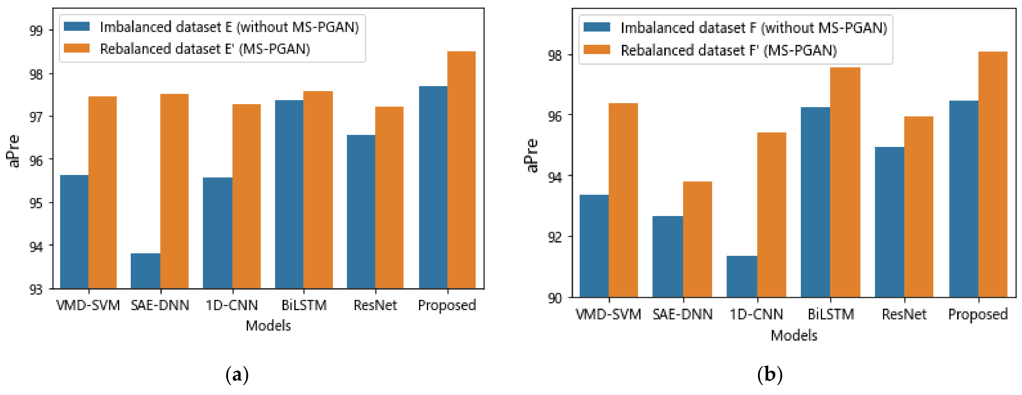
| Methods | Imbalance | Rebalance | ||||||
|---|---|---|---|---|---|---|---|---|
| 0.1 Ratio | 0.05 Ratio | 0.1 Ratio | 0.05 Ratio | |||||
| Dataset E | Dataset F | Dataset E’ | Dataset F’ | |||||
| aPre | aRec | aPre | aRec | aPre | aRec | aPre | aRec | |
| VMD-SVM | 95.62 | 95.50 | 93.35 | 93.33 | 97.44 | 97.42 | 96.38 | 96.33 |
| SAE-DNN | 93.81 | 93.75 | 92.67 | 93.61 | 97.52 | 97.43 | 93.79 | 93.77 |
| 1D-CNN | 95.56 | 95.47 | 91.36 | 91.25 | 97.26 | 97.22 | 95.40 | 95.28 |
| Bi-LSTM | 97.35 | 97.31 | 96.26 | 96.14 | 97.57 | 97.53 | 97.53 | 97.50 |
| Res-Net | 96.56 | 96.53 | 94.92 | 95.31 | 97.22 | 97.11 | 95.92 | 95.86 |
| Ours | 97.68 | 97.59 | 96.47 | 96.35 | 98.49 | 98.47 | 98.07 | 98.03 |
Publisher’s Note: MDPI stays neutral with regard to jurisdictional claims in published maps and institutional affiliations. |
© 2022 by the authors. Licensee MDPI, Basel, Switzerland. This article is an open access article distributed under the terms and conditions of the Creative Commons Attribution (CC BY) license (https://creativecommons.org/licenses/by/4.0/).
Share and Cite
Zheng, M.; Chang, Q.; Man, J.; Liu, Y.; Shen, Y. Two-Stage Multi-Scale Fault Diagnosis Method for Rolling Bearings with Imbalanced Data. Machines 2022, 10, 336. https://doi.org/10.3390/machines10050336
Zheng M, Chang Q, Man J, Liu Y, Shen Y. Two-Stage Multi-Scale Fault Diagnosis Method for Rolling Bearings with Imbalanced Data. Machines. 2022; 10(5):336. https://doi.org/10.3390/machines10050336
Chicago/Turabian StyleZheng, Minglei, Qi Chang, Junfeng Man, Yi Liu, and Yiping Shen. 2022. "Two-Stage Multi-Scale Fault Diagnosis Method for Rolling Bearings with Imbalanced Data" Machines 10, no. 5: 336. https://doi.org/10.3390/machines10050336
APA StyleZheng, M., Chang, Q., Man, J., Liu, Y., & Shen, Y. (2022). Two-Stage Multi-Scale Fault Diagnosis Method for Rolling Bearings with Imbalanced Data. Machines, 10(5), 336. https://doi.org/10.3390/machines10050336