Article

Feedforward–Feedback Controller Based on a Trained Quaternion Neural Network Using a Generalised HR Calculus with Application to Trajectory Control of a Three-Link Robot Manipulator †

1
Department of Information Systems Design, Faculty of Science and Engineering, Doshisha University, Kyoto 610-0394, Japan
2
Department of Intelligent Information Engineering and Sciences, Faculty of Science and Engineering, Doshisha University, Kyoto 610-0394, Japan
*
Author to whom correspondence should be addressed.
This paper is an extended version of our paper published in The 11th International Conference on Advanced Mechatronic Systems (ICAMechS 2021).
Machines 2022, 10(5), 333; https://doi.org/10.3390/machines10050333
Submission received: 30 March 2022 / Revised: 28 April 2022 / Accepted: 29 April 2022 / Published: 2 May 2022

Abstract

:
This study derives a learning algorithm for a quaternion neural network using the steepest descent method extended to quaternion numbers. This applies the generalised Hamiltonian–Real calculus to obtain derivatives of a real–valued cost function concerning quaternion variables and designs a feedback–feedforward controller as a control system application using such a network. The quaternion neural network is trained in real-time by introducing a feedback error learning framework to the controller. Thus, the quaternion neural network-based controller functions as an adaptive-type controller. The designed controller is applied to the control problem of a three-link robot manipulator, with the control task of making the robot manipulator’s end effector follow a desired trajectory in the Cartesian space. Computational experiments are conducted to investigate the learning capability and the characteristics of the quaternion neural network used in the controller. The experimental results confirm the feasibility of using the derived learning algorithm based on the generalised Hamiltonian–Real calculus to train the quaternion neural network and the availability of such a network for a control systems application.

1. Introduction

Recently, artificial intelligence, including machine learning, has been frequently used to find solutions for intractable problems in science and engineering and other fields, such as social science, economics and finance. Their ability to learn by example makes them capable of applicable solutions in real-world problems [1]. For instance, artificial intelligence could offer approaches for resolving robotics issues in control engineering, especially for autonomous robotics [2]. Neural networks (NNs) have been applied to solve numerous engineering problems over the last half-century due to their flexibility, learning capability and highly complex mappings [3]. Additionally, NNs incorporating deep-learning techniques and reinforcement learning integrating deep NNs are currently being used to handle challenging problems in the real world. They have demonstrated successful applications in many engineering fields [4,5]. Although deep learning is commonly utilised to deal with such problems, high-dimensional NNs, where all the network parameters and signals are based on complex and hypercomplex numbers including quaternion and octonion, have become an attractive alternative for handling such difficulties more efficiently and easily. Since the high-dimensional representation using such numbers can easily address multi-dimensional correlated data as a single entity and has many advantages, including parameter and computational efficiency [6], high-dimensional NNs have been explored to solve multi-dimensional and complicated problems [7,8,9,10,11,12].
A servo-level controller using a high-dimensional NN based on quaternion numbers was proposed in our previous work. Its characteristics for controlling nonlinear dynamical systems were investigated as a control system application of quaternion NNs (QNNs) [13,14,15]. Moreover, we found that the QNN outperformed the other networks in the learning and control of a three-link robot manipulator [16], such as real- and hypercomplex-valued NNs. It applies the steepest descent against the real-valued cost function defined by the error between the desired and system output to train the QNN. Since the cost function’s derivative to the quaternion variables representing the network parameters was required to derive the QNN’s learning algorithm, the derivative was calculated using the pseudo-derivative that calculates component-wise real derivatives concerning the real variables of the quaternion number. The pseudo-derivative is often used to derive the learning algorithm in many QNN applications, e.g., time-series signal processing, image processing, speech processing and pattern classification [10,17]. However, the formal derivatives of a real-valued function for the quaternion variables, including their involution, have been proposed using Hamiltonian–Real ( HR ) calculus, which is similar to the Wirtinger calculus relating complex numbers to quaternion numbers, to develop learning algorithms for signal processing using quaternion numbers [18]. Furthermore, a generalised form of the HR calculus called generalised HR (G HR ) calculus has been proposed to develop a more suitable learning algorithm [19]. Despite an increasing interest in learning algorithms based on the G HR calculus [20,21,22,23], its applicability on QNNs has not been adequately investigated. Moreover, practical, real-world applications using QNNs trained by such algorithms have not been fully explored, although such a QNN has been applied to control of a robot manipulator in a previous study [24].
Considering the aforementioned research gap, the main aim of this study is to determine how the specific properties of the learning algorithm based on the G HR calculus affect the QNN in control systems. In this study, the learning algorithm of a multi-layer QNN based on the G HR calculus is derived, and the possibility of using such a QNN in control system applications is explored. A servo controller based on the QNN is presented, where the input to the QNN consists of several input–output sets of the plant to handle plant dynamics and the output from the QNN is used to synthesise the control input to the plant. A feedback error learning (FEL) [25] framework extended to the quaternion numbers is employed to train the QNN-based controller. We used the QNN-based controller to perform computational experiments on the trajectory-tracking control of a three-link robot manipulator. We evaluated the feasibility and characteristics of the QNN trained by the learning algorithm based on the G HR calculus.

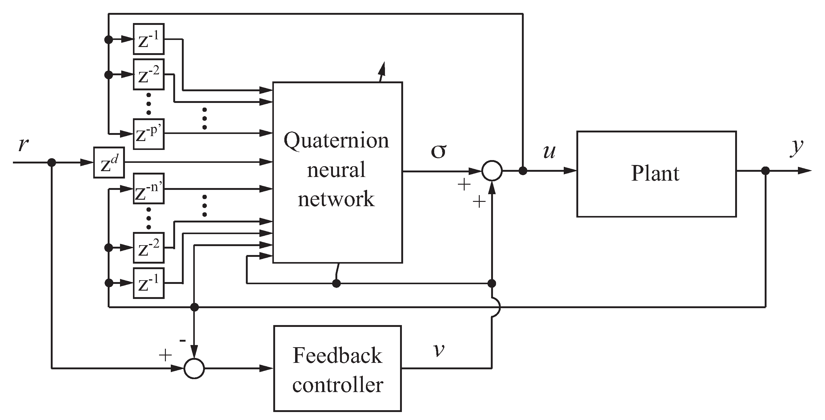
2. Feedforward–Feedback Controller Based on a Quaternion Neural Network

2.1. Generalised HR Calculus

Suppose the algebra of the quaternion numbers is H = { q q = q 0 + q 1 ı + q 2 j + q 3 κ , q 0 , q 1 , q 2 , q 3 R } using four real numbers and the basis { 1 , ı , j , κ } , where the units ı, j and κ satisfy Hamilton’s rules: ı 2 = j 2 = κ 2 = ı j κ = 1 , ı j = j ı = κ , j κ = κ j = ı and κ ı = ı κ = j . It forms a four-dimensional noncommutative, associative normed division algebra over real numbers.
Some basics of the HR calculus [18] are summarised first. Let the transformation for any quaternion number q be denoted as q μ = μ q μ 1 where μ is any nonzero quaternion number. The real variables of the quaternion number q i ( i = 0 , 1 , 2 , 3 ) can be expressed using the quaternion involutions: q 0 = 1 4 ( q + q ı + q j + q κ ) , q 1 = 1 4 ı ( q + q ı q j q κ ) , q 2 = 1 4 j ( q q ı + q j q κ ) and q 3 = 1 4 κ ( q q ı q j + q κ ) . Let f : H H be the quaternion-valued function f ( q ) = f 0 ( q 0 , q 1 , q 2 , q 3 ) + f 1 ( q 0 , q 1 , q 2 , q 3 ) ı + f 1 ( q 0 , q 1 , q 2 , q 3 ) j + f 3 ( q 0 , q 1 , q 2 , q 3 ) κ , the function f is real differentiable when the components f i ( i = 0 , 1 , 2 , 3 ) are differentiable as functions of real variables q i ( i = 0 , 1 , 2 , 3 ). If the function f is real differentiable, the HR derivatives of the function f to the involution are defined as follows:
f q = 1 4 f q 0 f q 1 ı f q 2 j f q 3 κ f q ı = 1 4 f q 0 f q 1 ı + f q 2 j + f q 3 κ f q j = 1 4 f q 0 + f q 1 ı f q 2 j + f q 3 κ f q κ = 1 4 f q 0 + f q 1 ı + f q 2 j f q 3 κ ,
and its conjugates are as follows:
f q * = 1 4 f q 0 + f q 1 ı + f q 2 j + f q 3 κ f q ı * = 1 4 f q 0 + f q 1 ı f q 2 j f q 3 κ f q j * = 1 4 f q 0 f q 1 ı + f q 2 j f q 3 κ f q κ * = 1 4 f q 0 f q 1 ı f q 2 j + f q 3 κ .
Consequently, the G HR derivatives of the function f with respect to q μ and q μ * ( μ 0 , μ H ) are defined as follows [19]:
f q μ = 1 4 f q 0 f q 1 ı μ f q 2 j μ f q 3 κ μ f q μ * = 1 4 f q 0 + f q 1 ı μ + f q 2 j μ + f q 3 κ μ ,
where { 1 , ı μ , j μ , κ μ } is the the generalised basis. Some properties of the G HR derivatives are given as follows:
p r o d u c t   r u l e : ( f g ) q = f q g g + f g q , ( f g ) q * = f q g * g + f g q * ,
r o t a t i o n   r u l e : f q μ = f μ q μ , f q * μ = f μ q μ * ,
c h a i n   r u l e : f ( g ( q ) ) q = μ { 1 , ı , j , κ } f g μ g μ q , f ( g ( q ) ) q * = μ { 1 , ı , j , κ } f g μ g μ q * .
where the functions f : H H and g : H H are real differentiable.
Using the G HR derivatives, Taylor’s theorem for quaternion-valued functions of quaternion variables can be formulated as a useful tool in calculus. The first-order Taylor series expansion of the function f ( q ) H is derived as follows:
f ( q + d q ) = f ( q ) + μ { 1 , ı , j , κ } f ( q ) q μ d q μ + O ( d q 2 ) .
If and only if the direction of the steepest descent d q is set to d q = η f q * = η f q * with the learning factor η R + , the following relationship can be obtained:
f ( q + d q ) f ( q ) μ { 1 , ı , j , κ } f ( q ) q μ d q μ = Re 4 f q d q 4 η f q 2 < 0 .
This yields the steepest descent method for quaternion numbers, which could be used as a learning algorithm for the QNN. Since the learning factor η defines a step size in the steepest descent, it functions to adjust the learning speed of the QNN.

2.2. Quaternion Neural Network

Considering a three-layer QNN with an input layer, a hidden layer and an output layer, the network’s input–output relationship can be given as:
σ l = j ω l j ψ ( i w j i s i ) ,
where s i H is an external input to the input layer’s i-th unit, w j i H is the connection weight between the input layer’s i-th unit and the hidden layer’s j-th unit, ω l j H is the connection weight between the hidden layer’s j-th unit and the output layer’s l-th unit, σ l H is the output layer’s l-th output and ψ : H H is the unit’s activation function in the hidden layer. The unit’s threshold in the hidden and output layers can be treated as a connection weight against a constant input.
Assuming that ϵ l H is the output error defined as ϵ l = t l σ l , where t l H is the teaching signal of the output layer’s l-th unit, the QNN’s connection weights are trained using the steepest descent method that minimises the following cost function defined using the norm of the output error:
E = 1 2 l ϵ l 2 .
Although the cost function is a real-valued function since the norm of the quaternion number is a real number, it is also a function of the quaternion number and its conjugate due to the definition of the norm: q = q q * where q H . Calculating the cost function gradient to the connection weights using the G HR calculus updates the connection weights according to the steepest descent method extended to quaternion numbers derived as follows:
ω l j = ω l j η E ω l j * = ω l j η 1 2 σ l ω l j ϵ l * * ϵ l * + ϵ l σ l * ω l j * = ω l j + 1 4 η ϵ l ν j * ,
w j i = w j i η E w j i * = w j i η 1 2 l σ l w j i ϵ l * * ϵ l * + ϵ l σ l * w j i * = w j i + 1 4 η l Re ϵ l ν j x j 0 * ω l j * + Re ϵ l ν j x j 1 * ω l j * ı + Re ϵ l ν j x j 2 * ω l j * j + Re ϵ l ν j x j 3 * ω l j * κ s i * .
where ν j = ψ ( x j ) is the hidden layer’s j-th output, and x j = i w j i s i is an internal state of the hidden layer’s j-th unit. These update rules are the back–propagation algorithm extended to quaternion numbers.

2.3. Feedforward–Feedback Controller

In this section, the QNN is used to design a controller which makes a plant output follow a reference signal. The control input to the plant is composed of both the QNN output and a feedback controller output in this controller because a FEL framework is introduced to train the controller’s QNN. To simplify designing the controller, the following discrete-time linear plant is considered:
y ( k + d ) = i = 0 n 1 α i y ( k i ) + i = 0 m + d 1 β i u ( k i ) ,
where y H is the plant output, u H is the control input, α i H and β i H are the plant’s coefficients, n and m are the plant orders, d is the dead time and k is the sampling number. The control input consists of the QNN output σ and the feedback controller output v, such as u ( k ) = σ ( k ) + v ( k ) . In defining the control error between the reference signal r and the plant output y: e ( k ) = r ( k ) y ( k ) , it can be rewritten using Equation (6) as:
e ( k + d ) = r ( k + d ) y ( k + d ) = β 0 { ξ T s ( k ) σ ( k ) } ,
where ( · ) T is the transpose operator,
ξ = β 0 1 1 α 0 α n 1 β 1 β p 1 β 0 T ,
s ( k ) = r ( k + d ) y ( t ) y ( k n + 1 ) u ( k 1 ) u ( k p + 1 ) v ( k ) T ,
and p = m + d . Assuming the control error becomes zero, the three-layer QNN is designed using the vector s ( k ) as the network’s input:
σ ( k ) = ω T ( k ) ψ ( W ( k ) s ( k ) ) ,
where the component of the matrix W H M × L comprises the connection weights between the input and hidden layers, and the component of the vector ω H M consists of the connection weights between the hidden and output layers. Here L is the number of units in the input layer defined as L = n + p + 1 , and M is the number of units in the hidden layer.
The connection weights are updated with the learning algorithm using Equations (11) and (12) at every sampling number, trained in real-time. Thus, the QNN acts as an adaptive controller. When the generalised δ -rule is applied to the QNN training by considering the plant’s dead time, the connection weight training in the controller is performed as follows:
ω ( k + 1 ) = ω ( k d ) η E ( k ) ω * ( k ) ,
W ( k + 1 ) = W ( k d ) η E ( k ) W * ( k ) .
where ( · ) * is the quaternion conjugate operator. The cost function, Equation (10), is defined using the feedback controller output instead of the output error; namely, the feedback controller output is minimised during the QNN training process according to the FEL. While the feedback controller is expected to keep the control system stable at the beginning of the QNN training process, the QNN comes to be a feedforward controller when the QNN training is ideally completed. Thus, such a controller is called a feedforward–feedback controller [26]. Figure 1 shows the resulting control system schematic.

2.4. Remarks on the Stability Condition of the Controller

The stability analysis of the QNN-based feedforward–feedback controller is important. However, it is generally difficult, owing to the nonlinearity of the controller and the plant, the noncommutative multiplication of quaternion numbers and the analyticity of the quaternion function used in the activation function. Therefore, the local stability condition of the controller is discussed by introducing the following assumptions:
(i)
The plant is represented by Equation (13), where the orders of the plant, the dead time and the sign of the high–frequency gain are known.
(ii)
The QNN’s activation function is a split-type function using a component-wise linear function even though it is not analytic in the field of quaternion number.
(iii)
The feedback controller is a P–controller, and the QNN’s connection weights allow the feedback controller output to be sufficiently small.
Using assumption (ii), the QNN, Equation (17) and the connection weight’s learning algorithm, Equations (18) and (19) can be rewritten as follows:
σ ( k ) = ω T ( k ) W ( k ) s ( k ) ,
W ( k + 1 ) = W ( k d ) + 1 2 η ω * ( k ) v ( k ) s H ( k ) ,
ω ( k + 1 ) = ω ( k d ) + 1 4 v ( k ) s H ( k ) W H ( k ) T ,
where ( · ) H is the Hermitian operator. Using assumption (i), the control error is represented by Equation (14). Substituting Equation (20) into Equation (14) yields:
e ( k + d ) = β 0 { ξ T ω T ( k ) W ( k ) } s ( k ) = β 0 ζ T ( k ) s ( k ) ,
where ζ T ( k ) = ξ T ω T ( k ) W ( k ) denotes the parameter error vector. Substituting Equations (21) and (22) into the parameter error vector and using the condition v ( k ) 1 obtained by assumption (iii) yields:
ζ T ( k + 1 ) = ξ T ω T ( k + 1 ) W ( k + 1 ) ζ T ( k d ) E 1 4 h η Ω ( k d ) ,
where
Ω ( k d ) = s ( k d ) s H ( k ) W H ( k ) W ( k d ) + 2 v 1 ( k ) ω T ( k d ) ω * ( k ) v ( k ) s H ( k ) ,
E is the identity matrix, and the feedback controller is assumed v ( k ) = h β 0 1 e ( k ) where h R + is the feedback gain. Assuming the function V ( k ) = ζ ( k ) 2 0 as the Lyapunov function candidate yields:
Δ V ( k ) = V ( k + 1 ) V ( k d ) = 1 4 h η ζ T ( k d ) Φ ( k d ) ζ * ( k d ) ,
where
Φ ( k d ) = Ω ( k d ) + Ω H ( k d ) 1 4 h η Ω ( k d ) Ω H ( k d ) .
Consequently, the stability of the parameter error vector ζ ( k ) is guaranteed when Δ V ( k ) 0 in Equation (26), namely, the matrix Φ ( k d ) is positive semi-definite. The matrix Φ ( k d ) is Hermitian because of its definition, so its eigenvalues are real numbers. This result clarifies the stability characteristics qualitatively, i.e., the stability depends on the learning factor, the feedback gain and the connection weight, which is strongly related to both the initial value and the convergence trajectory of the connection weight. Therefore, the brute force approach which changes the learning factor, the feedback gain and the connection weight’s initial values is necessary to find the stability condition quantitatively. Additionally, the convergence of the parameter error vector ζ ( k ) would not always satisfy the relationship ξ T = ω T ( k ) W ( k ) even though the feedback controller output becomes sufficiently small; namely, the control error approaches zero. The connection weight’s learning algorithm for the QNN using the steepest descent method primarily minimises the feedback controller output by matching the response between the plant output and the reference signal but does not estimate the true values of the plant parameter as in the adaptive control’s parameter identification. This shows that the QNN has a redundancy to realise the controller.

3. Computational Experiments

To investigate the feasibility and the characteristics of the QNN trained using the learning algorithm based on the G HR calculus in control systems application, computational experiments are performed to control a robot manipulator.

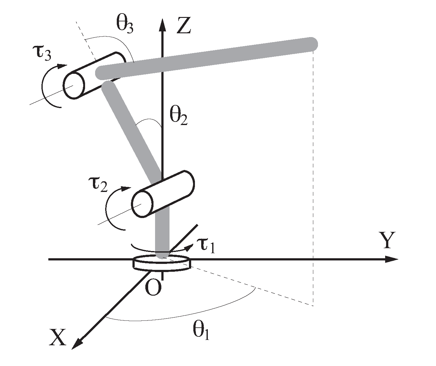
3.1. Robot Manipulator

The robot manipulator which has three joints, rotation–pivot–pivot type, shown in Figure 2, is the target plant controlled using the QNN-based feedforward–feedback controller. The motion equation of the robot manipulator is given as:
M ( θ ) θ ¨ + C θ ˙ + K ( θ , θ ˙ ) = τ ,
where θ R 3 is the joint angle vector, τ R 3 is the control torque vector, M ( θ ) R 3 × 3 is the inertia matrix, C = diag ( c 1 , c 2 , c 3 ) R 3 × 3 is the viscous matrix, and K ( θ , θ ˙ ) R 3 is the nonlinear force vector including the Coriolis force, centrifugal force, gravitational force and solid frictional force at the joints.
The control task is executed in the joint space, although the control objective for the robot manipulator is to ensure that the end-effector tracks the desired trajectory given in the workspace (Cartesian space). The desired position on the trajectory is transformed into the desired joint angles in advance through the robot manipulator’s inverse kinematics model. The movable range of each joint angle is restricted to avoid singular configurations and multiple solutions of the robot manipulator.

3.2. Controller Condition

In the QNN-based feedforward–feedback controller, the QNN has nine units in the input layer and one unit in the output layer. As described in Section 2.3, the input to the QNN s i ( k ) ( i = 1 , 2 , , 9 ) consists of the tapped–delay–line input–output sets of the robot manipulator as follows:
s 1 ( k ) = r 1 ( k + 1 ) ı + r 2 ( k + 1 ) j + r 3 ( k + 1 ) κ s 2 ( k ) = θ 1 ( k ) ı + θ 2 ( k ) j + θ 3 ( k ) κ s 3 ( k ) = θ 1 ( k 1 ) ı + θ 2 ( k 1 ) j + θ 3 ( k 1 ) κ s 4 ( k ) = θ 1 ( k 2 ) ı + θ 2 ( k 2 ) j + θ 3 ( k 2 ) κ s 5 ( k ) = θ 1 ( k 3 ) ı + θ 2 ( k 3 ) j + θ 3 ( k 3 ) κ s 6 ( k ) = u 1 ( k 1 ) ı + u 2 ( k 1 ) j + u 3 ( k 1 ) κ s 7 ( k ) = u 1 ( k 2 ) ı + u 2 ( k 2 ) j + u 3 ( k 2 ) κ s 8 ( k ) = u 1 ( k 3 ) ı + u 2 ( k 3 ) j + u 3 ( k 3 ) κ s 9 ( k ) = v 1 ( k ) ı + v 2 ( k ) j + v 3 ( k ) κ ,
where r i ( k ) is the reference signal to the joint angle θ i ( k ) , u i ( k ) is the control input, and v i ( k ) is the feedback controller output ( i = 1 , 2 , 3 ). Using the real variables of the imaginary part of the QNN output σ ( k ) = σ 0 ( k ) + σ 1 ( k ) ı + σ 2 ( k ) j + σ 3 ( k ) κ , the control input is synthesised by u i ( k ) = σ i ( k ) + v i ( k ) ( i = 1 , 2 , 3 ). The feedback controller output is given by v i ( k ) = γ h i T e i ( k ) where γ is the scale factor, h i R 2 is the feedback gain vector, e i ( k ) = [ e i θ ( k ) Δ i ( k ) ] T is the error vector, e i θ ( k ) is the control error in the joint space, and Δ i ( k ) = e i θ ( k ) e i θ ( k 1 ) is the difference of the control error ( i = 1 , 2 , 3 ). Consequently, the robot manipulator’s control torque is given by τ i ( k ) = T i u i ( k ) , where T i is the torque constant ( i = 1 , 2 , 3 ).

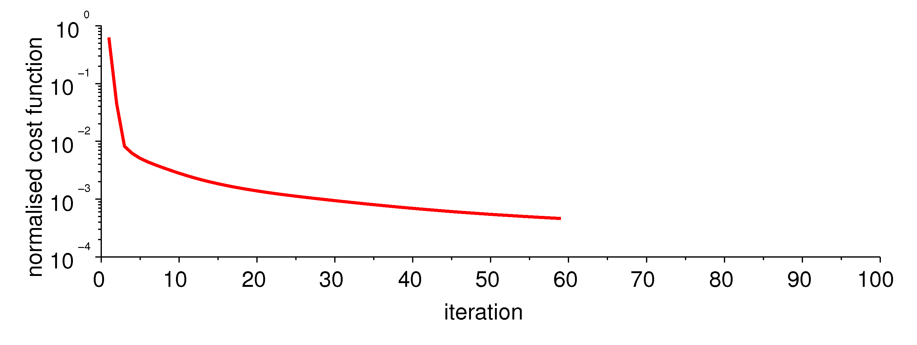
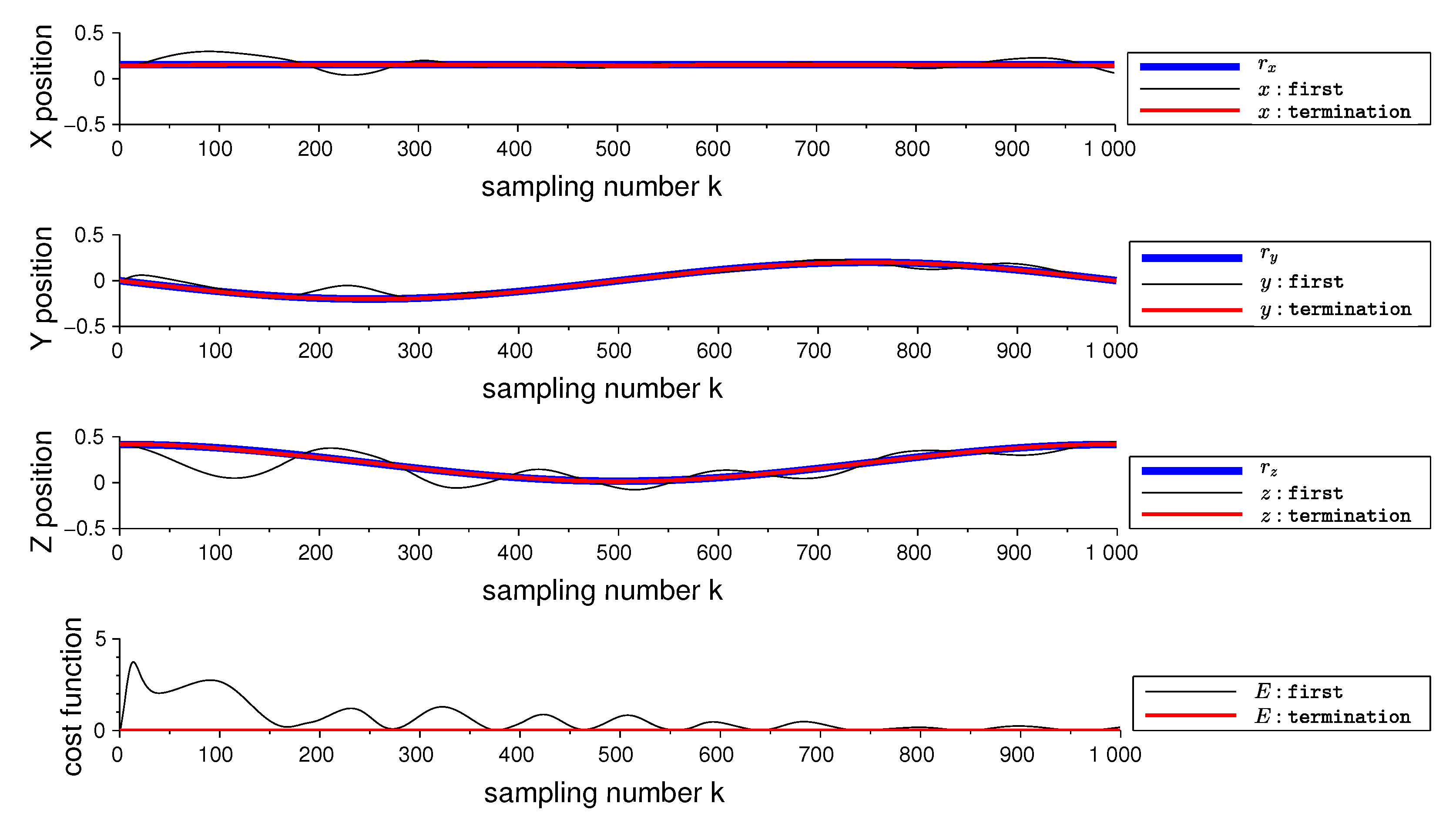
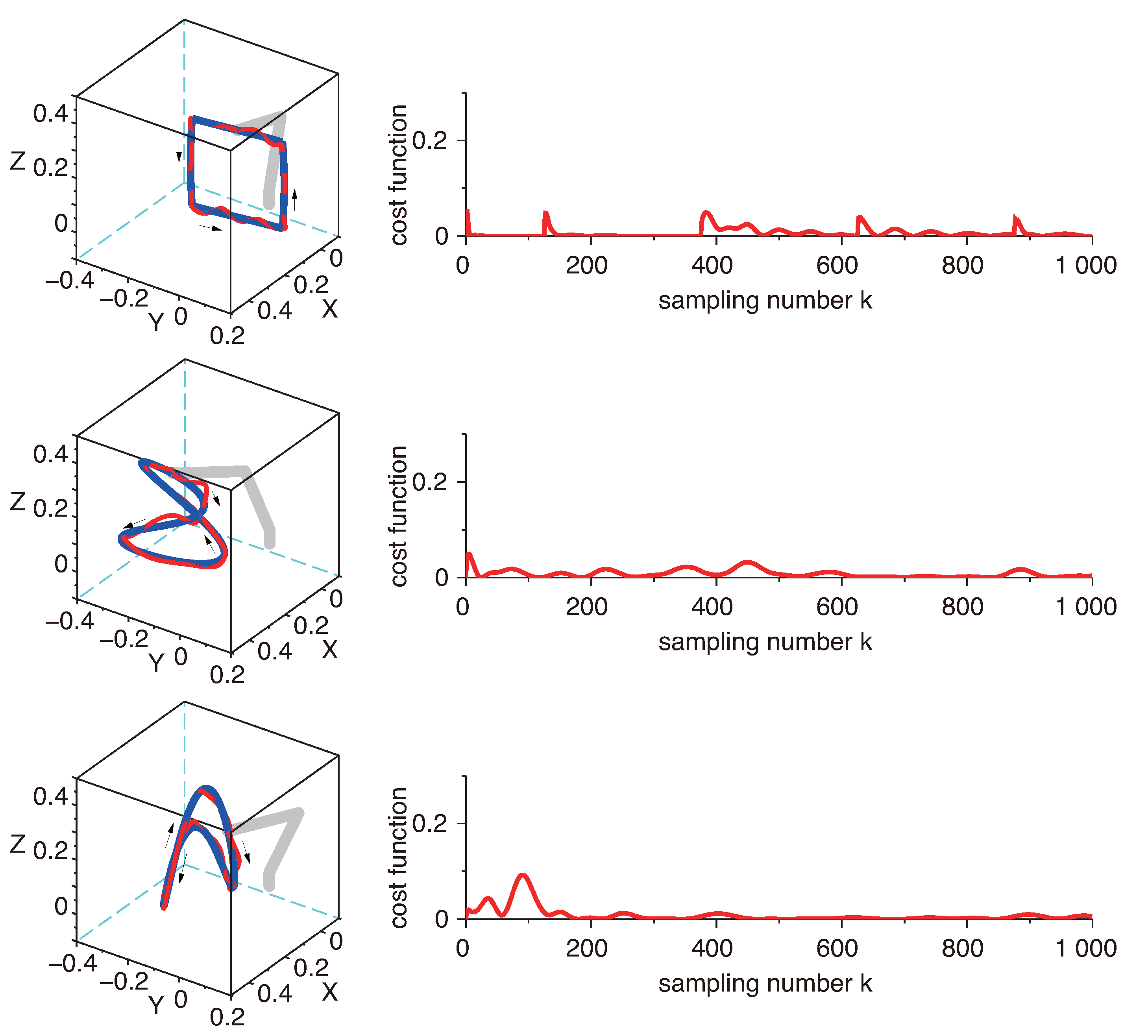
3.3. Numerical Simulations

The robot manipulator’s trajectory-tracking control experiments were conducted using the QNN-based feedforward–feedback controller. In the QNN, the unit’s activation function in the hidden layer is the split-type function using a component-wise sigmoid function. Each real variable of the quaternion numbers representing the connection weights was initialised randomly from the interval [ 1 , 1 ] . The FEL of the QNN was conducted in real-time. It was terminated when the normalised cost function, defined as the mean of the cost function, Equation (10), within one iteration of the desired trajectory, was less than the threshold value 0.0005 after five continuous iterations. The network training was restarted using the new connection weight’s initial values if the normalised cost function did not satisfy the termination condition after 100 iterations or if it tended to exceed a threshold and diverge during the training process. When the number of resets exceeded 10,000, the network training was defined as a failure. In the training process, the end-effector’s desired trajectory was a circle of radius 0.2 in the vertical plane parallel to the O–YZ plane. The trajectory consisted of 1000 data points per round, and one round was defined as one iteration. The feedback gains were h 1 = [ 4.0 0.04 ] T , h 2 = h 3 = [ 2.0 0.02 ] T , and the scale factor was γ = 1 . The torque constants was T i = 10 ( i = 1 , 2 , 3 ). The motion equation, Equation (28), was solved by the Runge–Kutta method with a 0.01 s step size in the numerical simulations. In the robot manipulator, the links 1, 2 and 3 were 0.05 m long and 0.4 kg mass, 0.25 m long and 0.2 kg mass, and 0.25 m long and 0.2 kg mass, respectively. The damping factor was c i = 0.005 ( i = 1 , 2 , 3 ), and the solid frictional forces were 0.2 Nm, 0.1 Nm and 0.1 Nm at the joints 1, 2 and 3, respectively. The robot manipulator’s initial condition was θ ( 0 ) = [ 0 π 12 5 π 12 ] T .
First, the feasibility of training the QNN with the proposed learning algorithm derived using the G HR calculus and controlling the robot manipulator using the QNN-based feedforward–feedback controller was investigated through numerical simulations. Figure 3 shows the change of the normalised cost function where the number of units in the hidden layer is two and the learning factor is 0.012. The normalised cost function decreases rapidly, and the network training is completed when the training’s terminating condition is satisfied. The normalised cost function decreases as the number of iterations progress and converge, indicating that it is possible to train the QNN in the control system. Figure 4 shows the response of the robot manipulator’s end-effector in the workspace and the variation of the cost function at each sampling time, indicating the responses at the first and termination of the training process shown in Figure 3. At the beginning of the training process, the end-effector does not follow the desired trajectory due to a lack of enough adaptation using the QNN. However, after the training converges, the end-effector could follow the desired trajectory; namely, the QNN-based feedforward–feedback controller achieves the control task. When the network training is terminated, the cost function at each sampling time is sufficiently small. This means that the major role of controlling the robot manipulator has shifted from the feedback controller to the QNN-based feedforward–feedback controller. These results confirmed that the QNN learning algorithm derived from the G HR calculus is functioning well. Therefore, it is feasible to apply the QNN-based controller for controlling the robot manipulator.
Next, the QNN’s learning characteristics were evaluated using two indexes: the number of iterations required to satisfy the network training termination condition and the number of resets during the training process. Here, 50 experimental results with different initial network weights were used to calculate these indexes. Table 1 summarises the number of iterations and resets when the number of units in the hidden layer is varied from one to four with a 0.012 learning factor. The index’s median and interquartile range are used instead of the mean and standard deviation because normal distribution is unobserved in these indexes according to the Shapiro–Wilk test with a 5% significant level. Additionally, multiple comparisons are conducted using the Steel–Dwass test. This result indicates that the number of units in the hidden layer has less effect on the learning speed if the network learning could progress, but the dependency on the connection weight’s initial values to proceed with the network training increases as the number of units increases. Table 2 summarises the number of iterations and resets when the learning factor is changed, where the number of units in the hidden layer is two. Increasing the learning factor improves the learning speed; however, the number of reset increases, namely, the dependency on the connection weight’s initial values to proceed with the network training increases. Furthermore, using a small learning factor increases the number of resets. This is because the first-order approximation of the steepest descent method makes the network training unstable with a large learning factor, whereas it is easy to reach the upper limit of the number of iterations with a small learning factor. Table 3 summarises the number of iterations and resets when the feedback gains are changed by the scale factor, where the number of units in the hidden layer is two and the learning factor is 0.012. Using smaller or larger feedback gains increases the number of resets although there is no statistical difference in the number of iterations. The network training did not converge when the scale factor was γ = 0.1 . Since the QNN output at the beginning of the network training affects the feedback controller as a disturbance, it is difficult to keep the control system stable with the smaller feedback gains. The control system becomes easily unstable with larger feedback gains due to the nonlinear characteristics of the robot manipulator because the feedback controller uses a simple error feedback. This result shows that an appropriate value of the feedback gain is required to proceed with the network training while ensuring the stability of the control system.
The control ability of the QNN-based feedforward–feedback controller was tested against untrained conditions after the QNN training process with the circular trajectory was completed. Figure 5 illustrates examples of the system response in the workspace where the desired trajectory and the initial condition of the joint angle were different from those set in the training process. Here, the number of units in the hidden layer was two, and the learning factor was 0.012. The FEL of the QNN was continued in real-time during the test. Although control errors can be observed partially around the curvature of the desired trajectory changes, the end-effector can follow the desired trajectory. The cost function sometimes increased with the control error but decreased soon as the sampling number progressed because the FEL can be performed stably in real-time after the pretraining with the circular trajectory. These results show that the QNN’s learning and generalisation capabilities are effective to compensate for the robustness of the control system against varying the robot manipulator’s experimental conditions.
Finally, the learning algorithm derived using the pseudo-derivative to calculate the cost function derivative to the network parameters was applied to train the QNN as a reference. Table 4 compares the number of iterations and resets the learning algorithm obtained using the G HR calculus with those obtained by the learning algorithm using the pseudo-derivative. A total of 100 experimental results were used to calculate these indexes. Here, there were two units in the hidden layer, and the learning factor was 0.012. To compare the learning characteristics under more severe conditions, the threshold value for terminating the network training was 0.0002. The learning algorithm using the pseudo-derivative attains a little faster learning speed, and the Mann–Whitney U test shows a statistical difference in the number of iterations. However, the learning algorithm using the pseudo-derivative requires many resets to proceed with the network training. Additionally, the network training by the learning algorithm using the pseudo-derivative sometimes failed to converge with the same value of the learning factor used in the learning algorithm using the G HR calculus. These results indicate that the learning algorithm using the G HR calculus can perform the network training stably with relatively less dependence on the connection weight’s initial values.

4. Conclusions

This study investigated a feedforward–feedback controller based on the QNN trained by the learning algorithm derived using the G HR calculus. In the QNN-based feedforward–feedback controller, the tapped–delay–line input–output sets of a plant were input to the QNN, and the control input to the plant was synthesised using the QNN output. A FEL framework performed at every sampling time was introduced to train the controller’s QNN to ensure that the plant output followed the desired output in real-time. Additionally, the local stability condition of the controller was analysed under linear assumptions of the QNN and plant. The result clarified how the learning factor, the feedback gain and the QNN’s connection weights affect the stability of the parameter error. Computational experiments on the trajectory-tracking control of a three-link robot manipulator using the QNN-based feedforward–feedback controller were conducted. Simulation results confirmed the feasibility of the learning algorithm derived using the G HR calculus to train the QNN, and the effectiveness of the QNN’s learning and generalisation capabilities to maintain the robot manipulator’s control performance. The experimentation of the QNN-based feedforward–feedback controller on an actual robot manipulator in real-world scenarios will be discussed in future work.

Author Contributions

Conceptualization, K.T.; methodology, K.T.; software, K.T. and E.T.; validation, K.T., E.T. and M.H.; formal analysis, K.T. and E.T.; investigation, K.T. and E.T.; resources, K.T. and M.H.; data curation, K.T. and E.T.; writing—original draft preparation, K.T.; writing—review and editing, K.T.; visualization, K.T. and E.T.; supervision, K.T. and M.H.; project administration, K.T.; funding acquisition, K.T. All authors have read and agreed to the published version of the manuscript.

Funding

This work was supported by JSPS KAKENHI Grant Number JP20K11980.

Institutional Review Board Statement

Not applicable.

Informed Consent Statement

Not applicable.

Data Availability Statement

Not applicable.

Conflicts of Interest

The authors declare no conflict of interest.

References

  1. Lu, Y. Artificial Intelligence: A survey on evolution, models, applications and future trends. J. Manag. Anal. 2019, 6, 1–29. [Google Scholar] [CrossRef]
  2. Ingrand, F.; Ghallab, M. Robotics and artificial intelligence: A perspective on deliberation functions. AI Commun. 2014, 27, 63–80. [Google Scholar] [CrossRef] [Green Version]
  3. Prieto, A.; Prieto, B.; Ortigosa, E.M.; Ros, E.; Pelayo, F.; Ortega, J.; Rojas, I. Neural networks: An overview of early research, current frameworks and new challenges. Neurocomputing 2016, 214, 242–268. [Google Scholar] [CrossRef]
  4. Dargan, S.; Kumar, M.; Ayyagari, M.R.; Kumar, G. A survey of deep learning and its applications: A new paradigm to machine learning. Arch. Comput. Methods Eng. 2020, 27, 1071–1092. [Google Scholar] [CrossRef]
  5. Wang, H.; Liu, N.; Zhang, Y.; Feng, D.; Huang, F.; Li, D.; Zhang, Y. Deep reinforcement learning: A survey. Front. Inf. Technol. Electron. Eng. 2020, 21, 1726–1744. [Google Scholar] [CrossRef]
  6. Alfsmann, D.; Göckler, H.G.; Sangwine, S.J.; Ell, T.A. Hypercomplex algebras in digital signal processing: Benefits and drawbacks. In Proceedings of the 15th European Signal Processing Conference, Poznan, Poland, 3–7 September 2007; pp. 1322–1326. [Google Scholar]
  7. Nitta, T. (Ed.) Complex–Valued Neural Networks—Utilizing High–Dimensional Parameters; Information Science Reference: Hershey, PA, USA, 2009. [Google Scholar]
  8. Hirose, A. (Ed.) Complex–Valued Neural Networks—Advances and Applications; Wiley-IEEE Press: Hoboken, NJ, USA, 2013. [Google Scholar]
  9. Tripathi, B.K. (Ed.) High Dimensional Neurocomputing—Growth, Appraisal and Applications; Springer: New Delhi, India, 2015. [Google Scholar]
  10. Parcollet, T.; Morchid, M.; Linares, G. A survey of quaternion neural networks. Artif. Intell. Rev. 2020, 53, 2957–2982. [Google Scholar] [CrossRef]
  11. García–Retuerta, D.; Casado–Vara, R.; Rey, A.M.; Prieta, F.D.; Prieto, J.; Corchado, J.M. Quaternion neural networks: State–of–the–art and research challenges. In Proceedings of the International Conference on Intelligent Data Engineering and Automated Learning, Guimaraes, Portugal, 4–5 November 2020; pp. 456–467. [Google Scholar]
  12. Bayro-Corrochano, E. A survey on quaternion algebra and geometric algebra applications in engineering and computer science 1995–2020. IEEE Access 2021, 9, 104326–104355. [Google Scholar] [CrossRef]
  13. Takahashi, K.; Isaka, A.; Fudaba, T.; Hashimoto, M. Remarks on quaternion neural network–based controller trained by feedback error learning. In Proceedings of the 2017 IEEE/SICE International Symposium on System Integration, Taipei, Taiwan, 11–14 December 2017; pp. 875–880. [Google Scholar]
  14. Takahashi, K. Comparison of neural network–based adaptive controllers using hypercomplex numbers for controlling robot manipulator. In Proceedings of the 13th IFAC Workshop on Adaptive and Learning Control Systems, Winchester, UK, 4–6 December 2019; pp. 67–72. [Google Scholar]
  15. Takahashi, K.; Watanabe, L.; Yamasaki, H.; Hiraoka, S.; Hashimoto, M. Remarks on control of a robot manipulator using a quaternion recurrent neural–network–based compensator. In Proceedings of the 2020 Australian & New Zealand Control Conference, Gold Coast, Australia, 25–26 November 2020; pp. 244–247. [Google Scholar]
  16. Takahashi, K. Comparison of high–dimensional neural networks using hypercomplex numbers in a robot manipulator control. Artif. Life Robot. 2021, 26, 367–377. [Google Scholar] [CrossRef]
  17. Parcollet, T.; Ravanelli, M.; Morchid, M.; Linarés, G.; Trabelsi, C.; Mori, R.D.; Bengio, Y. Quaternion recurrent neural networks. In Proceedings of the International Conference on Learning Representations, New Orleans, LA, USA, 6–9 May 2019; pp. 1–9. [Google Scholar]
  18. Mandic, D.P.; Jahanchahi, C.; Took, C.C. A quaternion gradient operator and its applications. IEEE Signal Process. Lett. 2011, 18, 47–50. [Google Scholar] [CrossRef]
  19. Xu, D.; Jahanchahi, C.; Took, C.C.; Mandic, D.P. Enabling quaternion derivatives: The generalized HR calculus. R. Soc. Open Sci. 2015, 2, 150255. [Google Scholar] [CrossRef] [PubMed] [Green Version]
  20. Xu, D.; Mandic, D.P. The theory of quaternion matrix derivatives. IEEE Trans. Signal Process. 2015, 63, 1543–1556. [Google Scholar] [CrossRef] [Green Version]
  21. Xu, D.; Gao, H.; Mandic, D.P. A new proof of the generalized Hamiltonian–Real calculus. R. Soc. Open Sci. 2016, 3, 160211. [Google Scholar] [CrossRef] [Green Version]
  22. Xu, D.; Xia, Y.; Mandic, D.P. Optimization in quaternion dynamic systems: Gradient, hessian, and learning algorithms. IEEE Trans. Neural Netw. Learn. Syst. 2016, 27, 249–261. [Google Scholar] [CrossRef] [PubMed] [Green Version]
  23. Popa, C.A. Learning algorithms for quaternion–valued neural networks. Neural Process. Lett. 2018, 47, 949–973. [Google Scholar] [CrossRef]
  24. Takahashi, K.; Tano, E.; Hashimoto, M. Remarks on feedforward-feedback controller using a trained quaternion neural network based on generalised HR calculus and its application to controlling a robot manipulator. In Proceedings of the 2021 (11th) International Conference on Advanced Mechatronic Systems, Tokyo, Japan, 9–12 December 2021; pp. 81–86. [Google Scholar]
  25. Kawato, M.; Furukawa, K.; Suzuki, R. A hierarchical neural-network model for control and learning of voluntary movement. Biol. Cybern. 1987, 57, 169–185. [Google Scholar] [CrossRef] [PubMed]
  26. Yamada, T. Remarks on feedback loop gain characteristics of adaptive type neural network feedforward feedback controller. In Proceedings of the SICE Annual Conference 2008, Tokyo, Japan, 20–22 August 2008; pp. 2244–2249. [Google Scholar]
Figure 1. Schematic of a QNN-based feedforward–feedback controller, where z is a shift operator, n = n 1 and p = p 1 .
Machines 10 00333 g001
Figure 2. Schematic of a three-link robot manipulator.
Machines 10 00333 g002
Figure 3. An example of the QNN’s training process.
Machines 10 00333 g003
Figure 4. An example of system responses in the workspace for controlling the robot manipulator using the QNN-based feedforward–feedback controller and the variation of the cost function. In the top three figures, the desired trajectory’s reference signal is drawn with a thick line, and the system response within the first iteration and the response that terminates the network training are drawn with thin and medium thick lines, respectively. In the bottom figure, the cost function within the first iteration and that which terminates the network training are drawn with thin and medium thick lines, respectively.
Machines 10 00333 g004
Figure 5. Examples of responses for controlling the robot manipulator using the QNN-based feedforward–feedback controller against untrained conditions, where the desired trajectory and the robot manipulator’s initial condition are as follows: in the top figure, a square and θ ( 0 ) = [ 0 π 12 π 2 ] T ; in the middle figure, a Lissajous curve and θ ( 0 ) = [ 3 π 16 π 9 π 3 ] T ; in the bottom figure, a Lissajous curve and θ ( 0 ) = [ 3 π 8 π 8 3 π 4 ] T . In each figure, the left figure illustrates the system response in the workspace where the desired trajectory and the response of the end-effector are drawn with thick and medium thick lines, respectively. The arrow indicates the direction of the end-effector’s movement and the stick figure illustrates the initial posture of the robot manipulator, whereas the left figure shows the variation of the cost function.
Machines 10 00333 g005
Table 1. Learning characteristics of the QNN concerning the number of units in the hidden layer.
Steel–Dwass TestIteration
1234Median (IQR)
Number of units1 42.5 (32.5–59.5)
2* 60.5 (38.5–81)
3 * * ns 63 (44.75–82.25)
4 * * nsns75 (60.75–87)
Steel–Dwass TestReset
1234Median (IQR)
Number of units1 48.5 (20.75–83.75)
2ns 75 (33.75–143.25)
3 * * * * 256.5 (92.25–634.5)
4 * * * * * * 1006.5 (317.75–2378.75)
(ns: not significant, * p < 0.05,** p < 0.01).
Table 2. Learning characteristics of the QNN concerning the learning factor.
Steel–Dwass TestIteration
0.0060.0120.0180.0240.030Median (IQR)
Learning factor η 0.006 72 (55.25–87.25)
0.012ns 60.5 (38.5–81)
0.018 * * ns 48.5 (37–67.5)
0.024 * * *ns 45 (29–66.25)
0.030 * * nsns43.5 (29.25–66)
Steel–Dwass TestReset
0.0060.0120.0180.0240.030Median (IQR)
Learning factor η 0.006 219.5 (91–681.5)
0.012 * * 75 (33.75–143.25)
0.018 * * ns 75.5 (31.75–141.25)
0.024ns 129 (47.75–270.5)
0.030ns* * * ns193.5 (64.5–392.25)
(ns: not significant, † p < 0.1, * p < 0.05, ** p < 0.01).
Table 3. Learning characteristics of the QNN concerning the feedback gain.
Steel–Dwass TestIteration
0.51210Median (IQR)
Scale factor γ 0.5 62.5 (45.25–78.5)
1ns 60.5 (38.5–81)
2nsns 71 (53–87.75)
10nsnsns71 (54.75–92)
Steel–Dwass TestReset
0.51210Median (IQR)
Scale factor γ 0.5 287.5 (124.5–432)
1 * * 75 (33.75–143.25)
2 * * ns 72 (27.75–119.25)
10* * * * * 483.5 (236.25–758.5)
(ns: not significant, * p < 0.05,** p < 0.01).
Table 4. Comparison of learning characteristics between the connection weight’s learning algorithms.
IterationResetSuccess Rate [%]
Median (IQR)Median (IQR)
G HR calculus69.5 (51.25–85.75)874.5 (460.5–2038.5)100
Pseudo–derivative45.5 (29.75–75.25)2106 (935–4656.5)94
Mann–Whitney U test * * * *
(** p < 0.01).
Publisher’s Note: MDPI stays neutral with regard to jurisdictional claims in published maps and institutional affiliations.

