Abstract
The ability of unmanned surface vehicles (USV) on motion control and the accurate following of preset paths is the embodiment of its autonomy and intelligence, while there is extensive room for improvement when expanding its application scenarios. In this paper, a model fusion of USV and preset path was carried out through the Serret-Frenet coordinate system. Control strategies were then scrupulously designed with the help of Lyapunov stability theory, including resultant velocity control in the presence of drift angle, course control based on the nonlinear backstepping method, and reference point velocity control as a virtual control variable. Specifically, based on USV resultant velocity control, this paper proposes respective solutions for two common scenarios through velocity planning. In a derailment correction scenario, an adaptive reference velocity was designed according to the position and attitude of USV, which promoted its maneuverability remarkably. In a dynamic obstacle avoidance scenario, an appropriate velocity curve was searched by dynamic programming on ST graph and optimized by quadratic programming, which enabled USV to evade obstacles without changing the original path. Simulation results proved the convergence and reliability of the motion control strategies and path following algorithm. Furthermore, velocity planning was verified to perform effectively in both scenarios.
1. Introduction
The ocean is one of the world’s most valued resource treasury, and ships have been an indispensable tool for human beings to approach and explore the ocean since ancient times. With the gradual increase of our desire to explore the unknown areas of the ocean and the complex water environment, people’s requirements for the performance of ships are also correspondingly strengthened, and the development of automation and intelligence of ships is one of the important areas that have received keen attention [1]. Among them, autonomy is an important attribute that USV can address by adaptively adjusting the output of its execution unit through a closed-loop control to achieve an ideal motion state. Intelligence is reflected in the USV’s ability to perceive and identify the environment, and respond through optimal decisions to adapt to the needs in that scenario. At present, due to its advantages and functions, USVs are gradually playing an irreplaceable role in scenarios such as water sampling and monitoring, anti-submarine warfare, target tracking, disaster management, and maritime search and rescue [2,3,4]. Any application scenario of USV is inseparable from the realization of the underlying motion control, whose goal is to control the movement of the USV in the spatial position. As the representative of USV motion control, path following is a basic function that mostly reflects the autonomy of USV. Undoubtedly, the fundamental research and design of a USV will determine the level of sophistication that can be achieved in such advanced devices integrating unmanned technology and artificial intelligence technology.
Modelling is the first step in USV motion control research, in which the accuracy and complexity of the model need to be taken into account. Mu D et al. [5] uses the Maneuvering Modeling Group (MMG) model to describe the motion characteristics of USV; the Nomoto model is derived to establish a transfer function describing the relationship between rudder angle and heading [6]. Thor I. Fossen has done a lot of remarkable work on USV. A maneuvering model he derived [7,8], which is widely used by scholars, intuitively reflects the maneuvering characteristics between the thrust and torque acting on the hull and the output of the hull motion state and has practical application value. Second, the USV motion control design aiming at the tracking of the preset path mainly revolves around the navigation and control algorithms. Based on the USV kinematic model, there are common guidance strategies such as Pure Pursuit, Line-Of-Sight (LOS) guidance [9] and Vector Field (VF) guidance [10]. Among them, LOS guidance is the most commonly used navigation method, and many researchers have improved it. Su Y et al. [11] considered both the time-varying sideslip angle and the time-varying ocean currents and proposed an Improved Adaptive Integral LOS (IAILOS). The control algorithm is based on the USV kinetic model. Common control strategies include PID control [12] and model predictive control (MPC) [13], which are more applicable in practice. In addition, robust controllers such as backstepping methods [14] and sliding mode control [15] are more accurate for nonlinear systems. Many scholars have comprehensively used the above methods and introduced new methods and ideas to carry out some optimization and improvement work. Li L et al. [16] proposed the extended state observer Line of Sight (ESO-LOS) guidance law, based on the extended state observer (ESO) prediction and compensation of the sideslip angle. Yu Y et al. [17] used finite time observers (FTOB) to predict the sideslip angle and kinetic uncertainties. Liu T et al. [18] established a ship tracking error model in the Serret-Frenet coordinate frame and proposed an improved LOS guidance algorithm using the tangential velocity of the desired path as the control input. Mu D et al. [19] designed an improved adaptive line-of-sight (ALOS) guidance law suitable for curve navigation based on the fuzzy optimization algorithm. It can be deduced that the drift angle of the USV motion is fully considered to make the results more realistic, and the Serret-Frenet coordinate frame can greatly simplify and clarify the path following the problem of the USV.
Based on the realization of motion control and path following, a USV can expand its application scenarios. A common situation is that the USV is likely to encounter moving obstacles such as other ships, offshore equipment and floating objects when navigating along a preset path on a relatively busy and complex water surface. Under certain constraints, it is of great significance to study the avoidance strategy of USV for these dynamic obstacles that violate its movement route. Song Lifei et al. [20] combined the velocity obstacle (VO) algorithm and the improved artificial potential field (APF) method to form a new two-level dynamic obstacle avoidance algorithm, in which emergency and non-emergency obstacle avoidance situations are carefully distinguished according to the standard whether the vehicle should move away from the obstacle immediately or not, so it can react with different situations efficiently. Ren J et al. [21] further considered the obstacle avoidance behaviour and the velocity obstacle region on the traditional velocity obstacle (VO) method, and further improved the method to make it easier for the ship to take avoidance actions. Faced with obstacle avoidance in complex unknown environments, Liu X et al. [22] combined Ant Colony Algorithm (ACA) and the Clustering Algorithm (CA) to propose a new auto-obstacle avoidance method, which can make full use of limited computing resources to automatically adjust and select smooth paths to avoid obstacles. Xia G et al. [23] determined the velocity window and course window of the USV through the dynamic window approach (DWA) and planned the ship’s local path to avoid collision based on modified quantum particle swarm optimization (MQPSO), which satisfies some rules of the International Regulations for Preventing Collisions at Sea (COLREGs). Chen Y et al. [24] proposed an improved ant colony optimization artificial potential field (ACO-APF) algorithm that takes into account both global and local path planning, and plans for dynamic obstacle avoidance during each step length analysis, ensuring that the hull is warned as soon as possible to avoid its action. Xia G et al. [25] proposed the nonlinear finite-time velocity obstacle (NLFVO) method to avoid obstacles whose motion laws cannot be determined. This method will analyze and predict the velocity state of the obstacles and select collision-free velocity for the USV based on the Gaussian mixture model (GMM) and Gaussian process regression (GPR). In the existing research, after evaluating the safe obstacle avoidance speed of the ship through methods such as velocity obstacle (VO), dynamic window approach (DWA) and artificial potential field (APF), the dynamic avoidance is generally completed by re-planning the path. However, this will obviously make the originally optimized preset path lose part of its meaning, and it is kind of inadvisable in some busy or narrow water scenes.
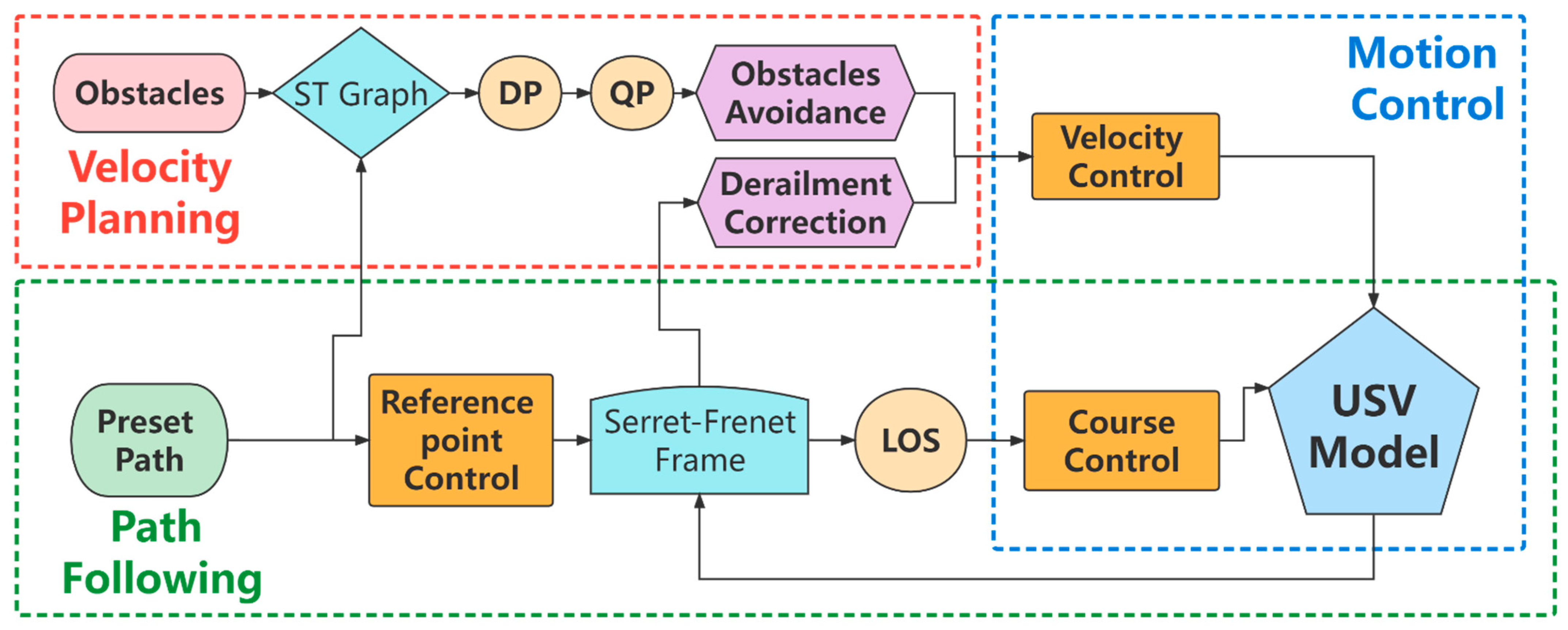
Thanks to a large number of excellent works by scholars, this paper can systematically study and discuss the motion control and path-following problems of USV, as well as the expansion of application scenarios based on velocity planning. Figure 1 is an illustration for the research framework for the concerned issues about USV established in this study. In this paper, the Serret-Frenet coordinate system is used in model processing, and the preset path and the motion of USV are combined into a new path following the error system. Then the system is decoupled into three aspects to carry out control strategies designed with the help of Lyapunov stability theory. Specifically, USV resultant velocity control in the presence of drift angle, USV course control based on nonlinear backstepping controller and LOS guidance law, and reference point velocity control as a virtual control variable are all carefully considered. Based on realizing reliable and comprehensive controls, this paper proposes solutions based on velocity planning about two common scenarios, i.e., derailment correction and dynamic obstacle avoidance. The derailment correction mainly reduces the movement velocity according to the position and attitude of the USV when it deviates from the desired route in order to reduce the deviation state as much as possible. Dynamic obstacle avoidance mainly searches for the optimal velocity curve by performing dynamic programming (DP) on the path-time graph generated by obstacles’ occupation (ST graph) and uses quadratic programming (QP) to fit the result. The optimization finally enables USV to avoid obstacles and keep following the original path only by adjusting its movement velocity. All the research results of this paper have been proven and verified through theoretical derivation and numerical simulation, which can provide some ideas and methods for scientific research and promotion in the field of autonomous unmanned system technology.
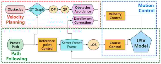
Figure 1.
Illustration for research framework of this paper.
2. Mathematical Models
The implementation of a reliable and comprehensive motion control strategy for USV is the basis for realizing a series of autonomous functions such as path following and obstacle avoidance. Therefore, this section firstly establishes a system model that can accurately represent the actual object and is not too complex at the same time, mainly including the USV kinetic model and kinematic model. To facilitate the research, the following hypotheses are given:
- Only 3-DOF movements of USV described by maneuvering theory are considered when modelling, i.e., surge, sway and yaw.
- The USV has no lateral push mechanism, that is, the drive input of the system only includes surge force and yaw moment.
- The USV surge velocity is constantly positive, that is, the parking and reversing of the USV are not considered.
2.1. USV Kinetic Model
The USV kinetic model reflects the maneuvering characteristics between the drive input acting on the hull and the output of the ship’s motion state. The underactuated USV kinetic model on the horizontal plane can be expressed by the simplified Fossen Model [26] that is widely used by scholars [27,28]:
where is the 3-DOF motion state vector of USV in the body coordinate system {B} with representing surge velocity, sway velocity and yaw angular velocity respectively. is the inertia matrix with representing the inertia coefficient containing the additional mass. is the Coriolis force-centripetal force matrix. is the damping matrix with representing the hydrodynamic damping coefficient. is the driving input matrix with and representing the thrust in the surge direction and the torque in the yaw direction respectively.
2.2. USV Kinematic Model in Serret-Frenet Coordinate Frame
The USV kinematic model describes the motion of USV as a particle in geometric space. In the inertial coordinate system, it is easy to obtain the kinematic equation of a USV moving on a horizontal plane:
where is the position and attitude state vector of USV in the Cartesian inertial coordinate system {I} with representing the coordinates and heading direction of the ship’s centre of gravity respectively. is a rotation matrix determined by the heading angle of the ship.
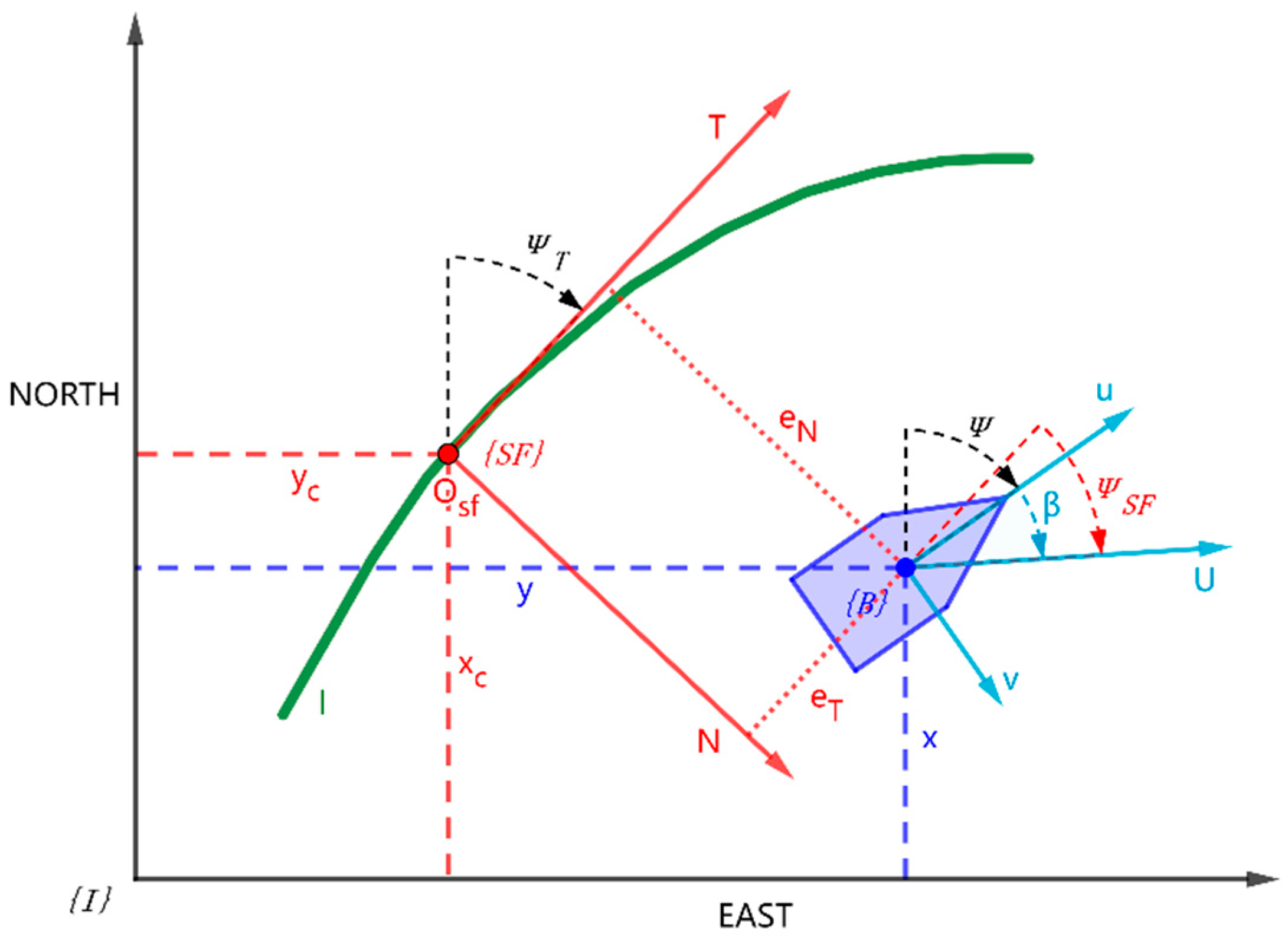
A Serret-Frenet coordinate system is introduced in this study to facilitate and simplify the USV path following the problem. As shown in Figure 2, the reference path is a parameterized planar two-dimensional curve l, and the curve parameter is denoted as p. The Serret-Frenet coordinate frame {SF} was established by selecting a reference point on path l, taking the tangential direction of the reference point as the vertical axis T and the normal direction of the reference point as the horizontal axis N.
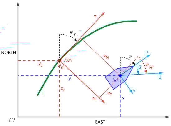
Figure 2.
USV path following in Serret-Frenet coordinate frame.
According to geometric relations, the kinematic equation of USV in {SF} frame is:
where and represent the position of the USV centre of gravity relative to the origin of the Serret-Frenet coordinate system. represents the angle between the direction of USV motion and the T-axis of the SF coordinate system. and represent the position of the path reference point relative to the origin of the inertial coordinate system, and represents the angle between the T-axis of the SF coordinate system and the North-axis of inertial coordinate system. is the drift angle of USV, indicating the angle between the actual movement direction of USV and the heading direction, which is essentially generated by the velocity of sway movement. It can be written as follows:
An error equation of the USV path following in the SF coordinate system can be obtained by differentiating the Equation (3):
where is the curvature of the desired path at the reference point, is the change rate of the reference point along the path curve, and is the resultant velocity of USV.
2.3. Problem Formulation
In this section, the kinetic model of USV, as well as the kinematic model under the {SF} frame, are established. Compared with the Cartesian coordinate frame, the data information that can characterize the preset path curve is integrated into the mathematical model of USV, making the target of the path following problem very clear and definite. It can also be noticed suggestively from the error Equation (5) that under the {SF} frame, the coordinate system is constantly changing along the path when the velocity of the reference point is not 0. In fact, the selection of reference points can be completely arbitrary, because there is no concrete physical object to manipulate the reference point. The inspiration brought by this is that the moving velocity of the reference point can be regarded as a virtual control variable, and an appropriate control law can be designed to make the position of the reference point change according to the expectation for the system’s stability. As a result, the original underactuated system model is supplemented into a fully-actuated one with three inputs and three outputs in terms of the quantity of inputs and outputs.
The USV path following problem can then be described as designing control laws for
to let
where two control variables and from USV actuators have output limits, and , , are the initial state of USV. , and all converging to zero means that USV will finally move to the origin of the coordinate system and keep its forward direction consistent with the vertical axis under the view of {SF} frame.
3. Control Strategies
Based on introducing a virtual control variable, the system model of the USV path following is still a strongly coupled and nonlinear research object. This paper mainly uses Lyapunov stability theory, with the help of the idea of nonlinear backstepping controller design and LOS guidance design, to develop relatively independent control strategies under the {SF} frame: First, the control strategy of USV thrust with fully considering the existence of drift angle is designed, so that the real moving velocity of USV can be controlled; Second, the control strategy of USV torque is designed so that the USV moving course can follow the expected course generated by the guidance law. Thirdly, the control strategy of reference point movement is designed to ensure that the position of USV can converge to the reference point which is precisely on the curve path.
3.1. Resultant Velocity Controller Design
Different from other studies that set the USV velocity as a constant by default, or fixed the thrust output as a constant, or only controlled the surge velocity u, resultant velocity controller (RVC), without ignoring the drift angle, drives the USV according to the desired actual velocity by controlling the thrust force based on the full modelling of the USV system. This also makes it possible to optimize the USV path following and dynamic obstacle avoidance based on velocity planning.
Without ignoring the drift angle, that is, taking full account of the sway velocity, the derivative of can be achieved:
Substituting the surge acceleration and the sway acceleration from USV kinetic Equation (1) into Equation (8) leads to:
Applying the Lyapunov Direct Method on Equation (9) and the specific derivation process can be seen in Appendix A. Then the control law of RVC is designed as:
where the positive parameter is the controller gain.
3.2. Nonlinear Backstepping Course Controller Design
The main function of the nonlinear backstepping course controller (NBCC) is to track the expected value by controlling the USV torque. In this study, the LOS algorithm, which is widely used in path-following problems, is used to generate the desired course :
where is a parameter representing the forward-looking distance in LOS guidance law. This traditional LOS algorithm is simple and reliable for solving the path following problem with intuitive geometric significance. Its essence is a kind of planning for the convergence process of course tracking, which guides the object to approach the preset path by establishing the constraint between transverse error and course.
The backstepping method is a design idea that realizes the stabilization of the chain of integrator system by constructing Control-Lyapunov Function (CLF) recursively. At the same time, the course control problem of the USV path following can be solved reliably by using feedback linearization control law design. According to the USV mathematical model, yaw angular velocity can be controlled by changing the torque, which is also the main variable affecting the course of USV. The specific derivation process can be seen in Appendix B. The course control law for the path following problem is:
where both positive parameters and are the controller gains.
3.3. Path Reference Point Controller Design
The selection of {SF} frame provides an additional virtual control variable for the USV path following system in kinematics, i.e., the moving velocity of path reference point . The essential purpose of controlling the moving velocity of the path reference point is to enable USV to select the appropriate reference point on the path in real-time and establish an SF coordinate system based on this point. In this coordinate system, together with USV moving velocity and course control, the established kinematic error equation can converge to zero. Its geometric significance is to clarify the relative position and angle differences between the USV and the preset path and provide a reference for the positioning of the forward-looking distance in LOS guidance.
According to the error Equation (5), with the help of the Lyapunov Direct Method, the control law of the reference point’s movement velocity is:
where the positive parameter is the controller gain.
It should be pointed out that the natural parameter equation of curve is often difficult to obtain, but for the two-dimensional curve equation expressed by general parameter , there is an operational relationship between arc length s and parameter p:. Substitute it into Equation (13) and the control law regarding the velocity of path curve parameter as the control variable can be obtained:
where and are the derivatives of the curve equation with respect to the parameter p.
4. Stability Analysis
In Section 3 of this paper, the corresponding control law is designed regarding the thrust and torque of USV and the selection of reference points in the SF coordinate system. This section mainly analyzes the stability of the designed control law based on the Lyapunov stability criterion and finally proves the convergence of USV motion control and path following.
4.1. Stability Analysis of Velocity Control
The error between the resultant velocity of USV and the expected value in RVC is written as :
Differentiating the equation above and substituting the result into Equation (9) and control law (10) leads to:
It obviously comes to a time-domain solution that decays exponentially to zero when the parameter is positive, which indicates that will eventually approach . It proves that USV can advance according to the expected velocity value given by the outer loop in actual motion.
4.2. Stability Analysis of Course Control
Based on the derivation process of backstepping presented in Appendix B, a new system was constructed using the error equation of USV motion direction and angular velocity:
It can be found that the USV course error system becomes a linear system with an equilibrium point of after adopting the backstepping method combined with feedback linearization in controller design. Upon analyzing the eigenvalue of the system matrix , there is:
When the parameters and are positive, the solutions of the eigenvalues and of the error system matrix all have negative real parts, which indicates the fact that the linearized USV course error system is a stable system that can converge to zero, which proves that USV can track the desired course in actual motion.
4.3. Stability Analysis of USV Path Following
Based on the algorithm design of USV thrust and torque output, the actual movement velocity and direction are stably controlled at the kinetic level, that is, the states of USV motion are respectively satisfied and with convergence proved. On this basis, designing the control law of the reference point in the SF coordinate system let the error variables in the system (5) converge stably to zero, which enables the USV motion path to track the preset curve from the kinematic level. The proof is as follows:
Define a Lyapunov function :
Differentiating the equation above and substituting the control strategy (13) of reference point velocity leads to:
And according to the designed LOS guidance law (11), there is:
Substituting the Equation (21) into Equation (20) leads to:
On the whole, the error Equation (5) of USV path following under {SF} frame has equilibrium point of . Obviously, when and both have positive values, is positive definite and is negative definite. Then the USV path following the error system converges stably to the equilibrium point when applying the Lyapunov stability theory, which ultimately proves that USV can move from any initial state to the preset path curve in the inertial coordinate system.
5. Scenario-Oriented Velocity Planning
In this study, the resultant velocity of USV can be controlled to adjust adaptively with the change of given expected value by the design of RVC. Taking advantage of this feature, velocity planning can be carried out for a USV to realize various functions of autonomous movement and meet the needs of different scenarios.
5.1. Velocity Planning for Derailment Correction Based on USV Position and Attitude
Derailment generally refers to the fact that the USV deviates from the preset path to be tracked. There are two common adverse situations: First, the initial position and attitude of the USV are far from the starting point of the path to be tracked; Second, the course or even position of the USV deviates from the original path when the USV encounters sudden external disturbances during driving. For ships with underactuated properties, reducing the velocity appropriately will be beneficial to contract the turning radius under the condition of limited steering torque input, which is helpful to complete derailment correction in a small scale of space. This paper gives a scheme of USV velocity planning for derailment correction based on its position and attitude to enhance the path following performance. The reference velocity value satisfies the following:
where parameter represents the variation range of the reference velocity. and are weight parameters of USV deviate angle and distance respectively. Parameter represents the lowest velocity of USV. All the above parameters are positive. With the design on reference velocity of RVC, the USV’s resultant velocity can be adjusted adaptively to the current position and attitude within a certain range. Specifically, when the deviate angle or distance of the USV increases under {SF} frame, RVC will reduce the reference value of the USV’s moving velocity until the lowest value ; When the USV position converges to the preset path, the RVC increases the expected velocity to the value , which is also exactly the cruising velocity of the USV along the preset path.
5.2. Velocity Planning for Dynamic Obstacle Avoidance Based on ST Graph Optimization
The ST graph takes time as the horizontal axis and the distance along the preset path curve as the vertical axis. The dynamic obstacle that may overlap with the path is projected onto the path, so as to generate the corresponding ST boundary. The area enclosed is the two-dimensional expression of the path length and time occupied by this dynamic obstacle. All obstacles that may encroach on the path can be in accordance with the rules of geometry to solve their projection into the ST graph, so as to determine the occupied range of time and space of the path. Therefore, as long as a monotone increasing curve that bypasses all obstacle blocks as well as satisfies certain conditions of constraints and optimization can be searched out in the ST graph, obstacle avoidance of unmanned mobile devices can be safely ensured. The derivative of such searched curve is exactly the velocity curve, and the searching process is the velocity planning process facing the dynamic obstacle scenario.
In this study, the projection of the dynamic obstacle on the ST graph is obtained by solving the implicit function:
where and describe the real-time position of the ith obstacle. and describe the real-time position of USV. and represents the collision radius of obstacles and USV, respectively.
The feasible region and obstacle region for searching are divided according to the conservative principle after rasterizing the ST graph with appropriate accuracy. Meanwhile, the upper and lower limits of USV velocity and acceleration were used as constraints to further limit the feasible region for searching. At this point, the route search of the discretized ST graph is transformed into an optimization problem to solve the multi-stage decision process. This paper adopts the dynamic programming (DP) algorithm to solve the problem, and defines the cost function between each connected state according to the following formula:
where is the acceleration of USV actual velocity, is the jerk of movement, and are their weight coefficients, respectively.
The result from DP is optimal under the selected dispersion with respect to the smoothness of velocity variation, but the derivative of the searched curve is often discontinuous, which means that the reference value of USV movement velocity will jump. USV then will go through a transitional stage of breaking away from the desired state in the actual situation, resulting in the risk of being out of control. In this study, a series of quintic polynomial curves are used to smooth the curve searched by DP. In addition to the constraints from position, velocity and acceleration, boundary condition constraints of the start point of the ST curve and the connection points of each stage are also considered. The cost function containing acceleration, jerk and position error is defined as follows, and the corresponding coefficients of the polynomial are solved by quadratic programming (QP) to complete the smooth optimization of velocity planning:
where is the total number of stages in DP, is the acceleration of USV motion in each stage, and for jerk. Expression represents the difference between the position of the ST curve obtained by DP against the position after QP optimization. , and are the weight coefficients of the three respectively.
6. Numerical Simulation Results
The research ideas of USV motion control, path following and obstacle avoidance proposed in this paper have been proved theoretically. This section will further verify the convergence and effectiveness of relevant algorithms through computer numerical simulation with MATLAB&SIMULNK. Specifically, the motion modelling under the framework of USV combined with the SF coordinate system is first carried out. The relative control algorithm for USV resultant velocity, course and path reference point velocity as a virtual control variable is programmed. Meanwhile, LOS guidance law is also introduced. Then, a series of simulation experiments were carried out around the velocity planning schemes applied in the two scenarios to comprehensively verify the control effect of USV autonomous navigation studied in this paper. The USV model used in the simulation experiment is described by the following parameters: , , , , , .
6.1. Simulation Results of Derailment Correction
Draw up a preset path curve C1 for the lane change operation: , where . Set an initial state where the USV is deployed deviate significantly from the start of the path: , , m/s, and the rest initial values of motion states are all set to zero. There are limits on USV actuators: , . The following parameters are used to configure the velocity planning for derailment correction based on USV position and attitude: . At the same time, a specific zone crossing the desired path is assumed where there are disturbances caused by external environment, compelling the USV to change its course angle by 30°. The initial value of the parameter of the preset path is , and the forward-looking distance in LOS guidance law is m. Controller gain of RVC is . Controller gains of NBCC are . Controller gain for path reference point is .
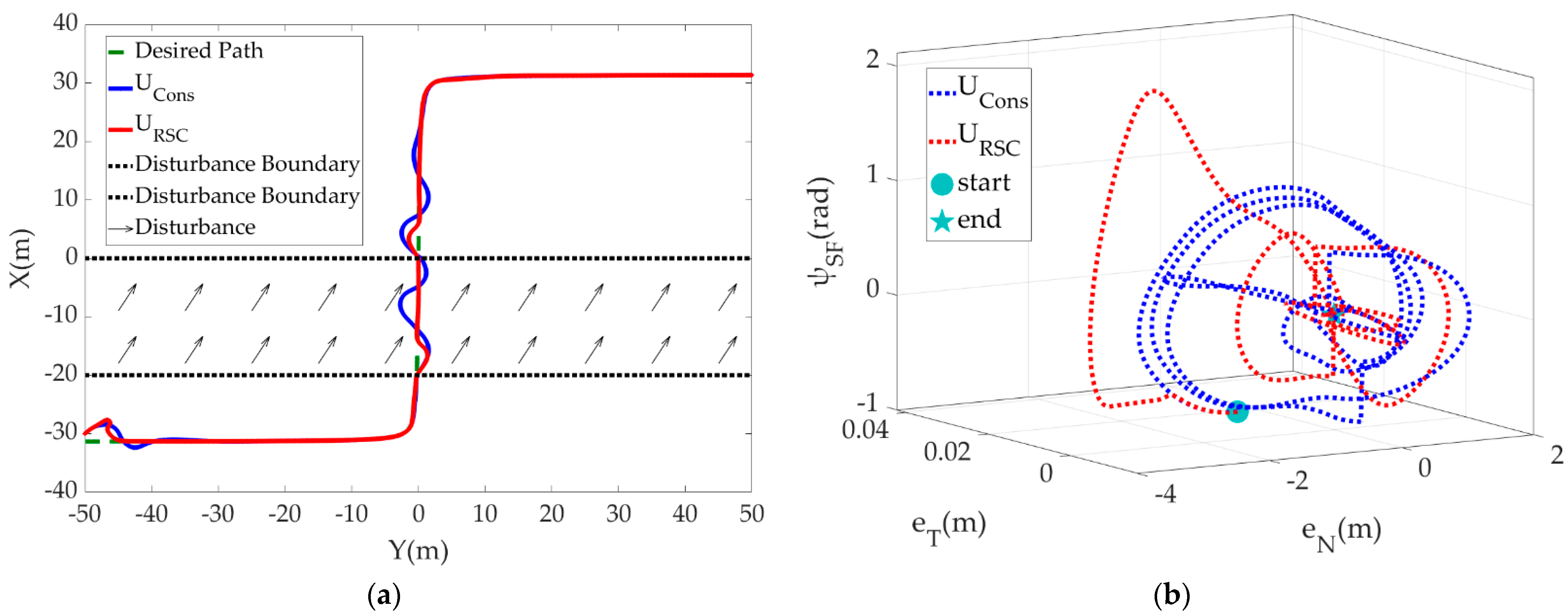
Figure 3 shows the following effect of USV on a lane-changing path in the inertial coordinate system and the Serret-Frenet coordinate system, respectively. Two derailment scenarios under the influence of initial state deviation and external disturbances are also set up. In Figure 3a, the green dotted line is the preset path. The black arrow area shows the zone where disturbance interferes with the course of USV. The blue line shows the path following and derailment correction effects of the USV moving at a constant velocity. The red line shows the effect of the USV moving at an adaptively adjustable velocity based on its position and attitude. In Figure 3b, the cyan circle represents the start point of USV in the Serret-Frenet coordinate system, and the pentacle represents the endpoint (both points of the two groups of comparative experiments are consistent). The blue dotted line indicates the convergence effect of constant velocity moving, and the red dotted lines indicate the convergence effect of variable velocity moving.
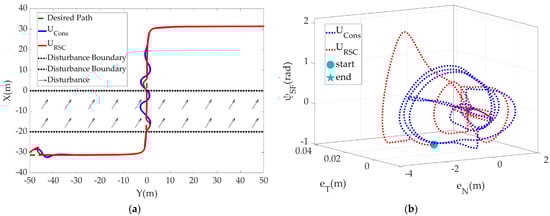
Figure 3.
Results of USV path following for C1: (a) Perspective in the inertial coordinate system; (b) Perspective in the Serret-Frenet coordinate system.
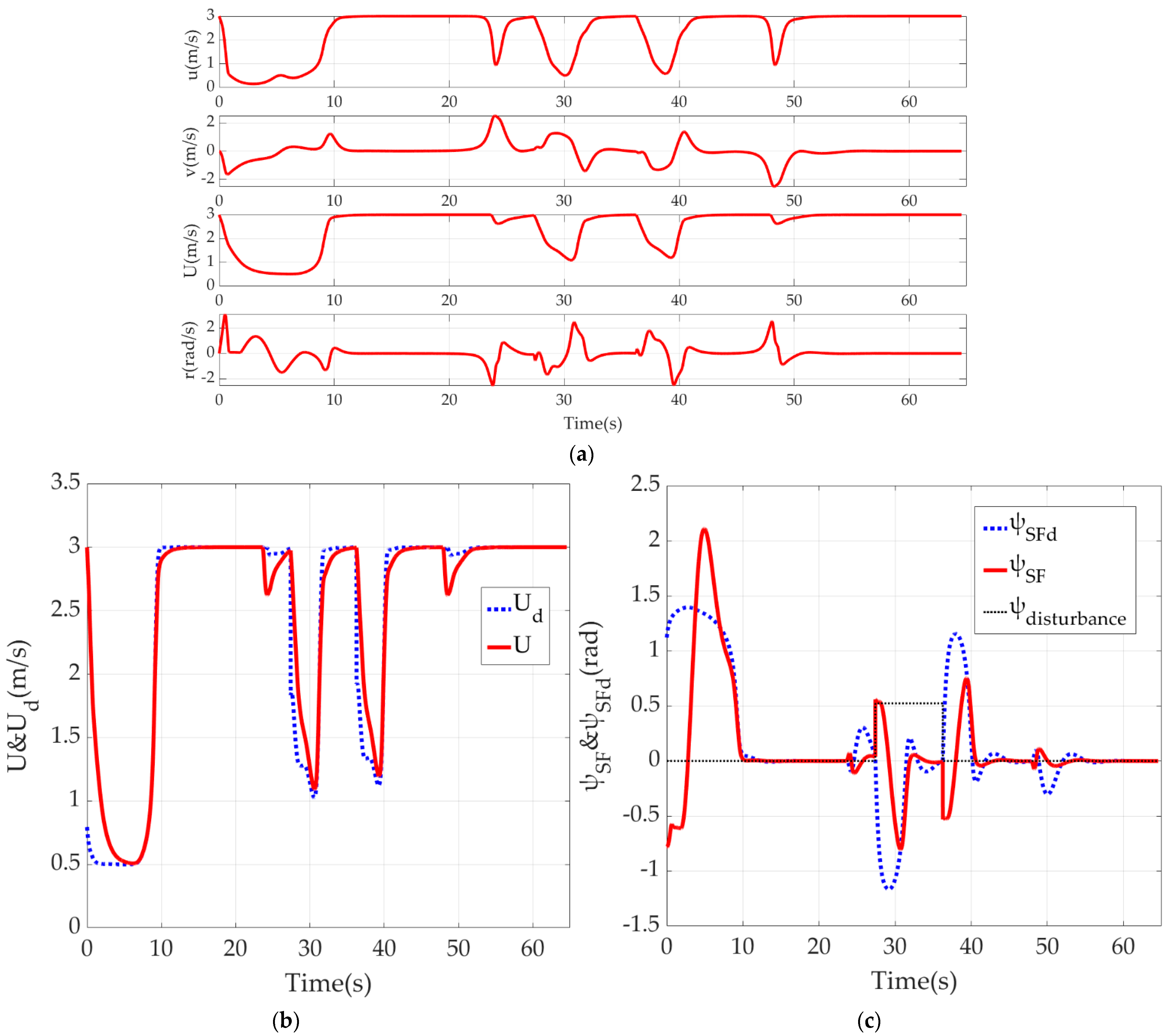
Figure 4 shows a series of data related to the underlying motion control of the USV velocity planning based on its position and attitude in path following and derailment correction. Figure 4a records the rate of motion on 3-DOF of surge, sway and yaw, and the real moving velocity. Figure 4b,c shows the control effect towards set values by an outer loop of RVC and NBCC, respectively. Figure 4d shows USV thrust and torque output under finite-amplitude conditions. Figure 4e is the reference point moving velocity along the path curve represented by a general parameter, which also serves as a virtual control variable introduced for the underactuated USV path following problem. Figure 4f is the position of the reference point at the corresponding time.
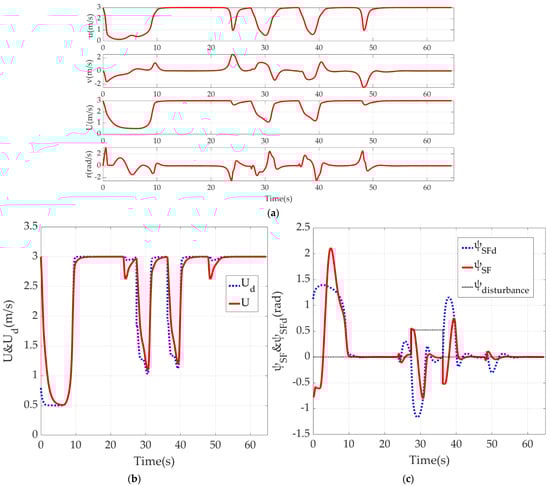
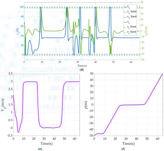
Figure 4.
Results of USV underlying motion control: (a) USV 3-DOF motion data; (b) Tracking effect of RVC on expected velocity; (c) Tracking effect of NBCC on LOS guidance law; (d) Thrust and torque output; (e) Reference point moving velocity on path curve; (f) Reference point position on path curve.
6.2. Simulation Results of Dynamic Obstacle Avoidance
Draw up a preset path curve C2 in the polynomial form: , where . Set the initial position and direction of the USV to be consistent with the start point of the path curve, while the initial velocity is m/s. In this scenario, two dynamic obstacles are moving across the preset path straightly. The starting position and velocity vectors of the obstacle are respectively , and , . Their collision radius is assumed to be 2 m and 4 m. USV’s collision radius is assumed to be 2 m. The upper and lower moving velocities are respectively assumed to be 3 m/s and 0.1 m/s, while accelerations are 3 m/s2 and −2 m/s2. The rest configurations of the controller coincide with the ones in Section 6.1.
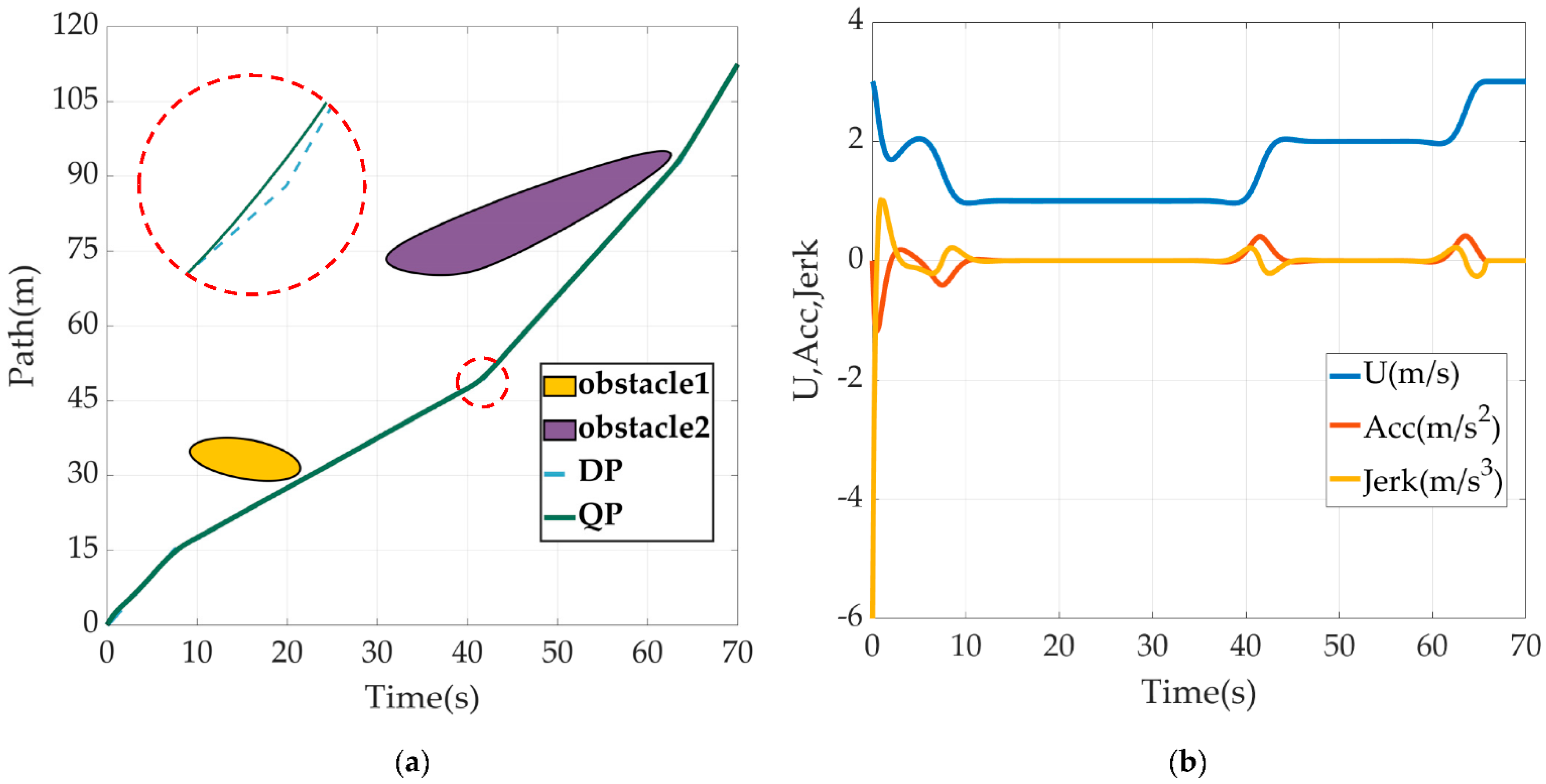
Figure 5 is the ST graph generated by the projection calculation of obstacles and the velocity curve obtained after DP and QP optimization. In Figure 5a, the yellow and purple blocks represent the Spatio-temporal domain of the preset path occupied by two dynamic obstacles. DP rasterizes the ST graph according to the discretization degrees of 0.5 s and 0.5 m, and then conducts search optimization for the 140 discrete stages according to constraints and cost functions to obtain the path-time curve represented by segment lines, namely the blue dotted line in the figure. The curve derivative of DP search has mutations, which is not conducive to practical application. Next, the curve was smoothed by a series of quintic polynomials, and their coefficients are solved by QP according to constraints and cost functions. Finally, the optimized green curve in the figure was obtained, so the velocity planning of USV for dynamic obstacle avoidance was completed. As can be seen from Figure 5b, the velocity, acceleration and jerk of the USV’s movement are equipped with smooth continuity after QP for optimizing, which can be used as the reference input value of RVC in practical application.
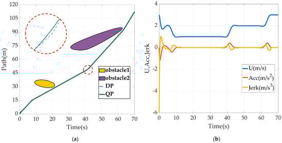
Figure 5.
Velocity planning based on ST graph. (a) Results of DP & QP; (b) Reference input values of RVC generated from QP.
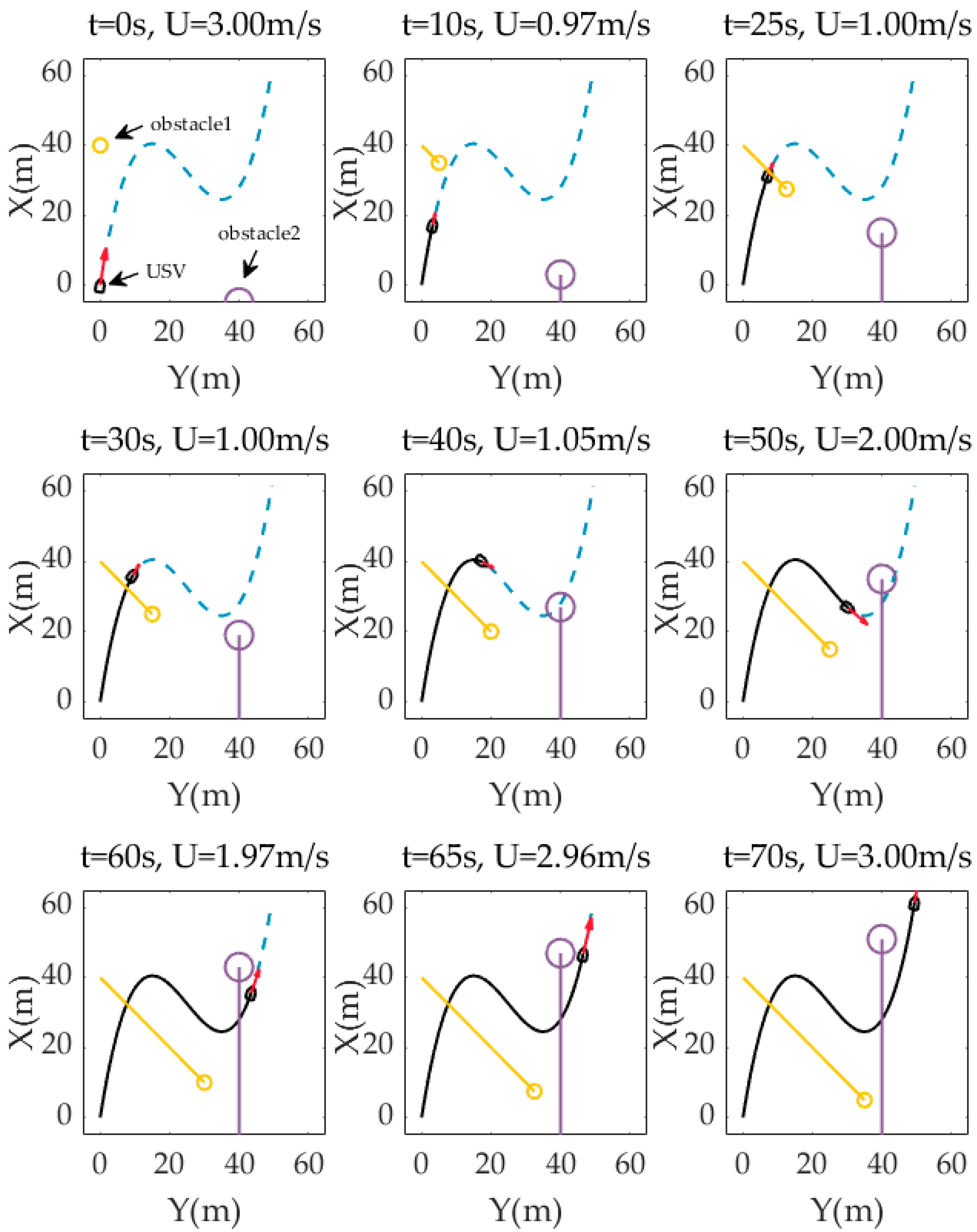
Figure 6 is a time diagram of the USV path following and dynamic obstacle avoidance based on ST graph optimization. The dotted blue line is the preset path to be tracked, and the solid black line is the actual trajectory of the USV. The red arrow in front of the USV mark indicates the direction and velocity of its actual movement. The yellow and purple circles are the two moving obstacles crossing the path, and the tail lines of the corresponding colours are their respective trajectories.
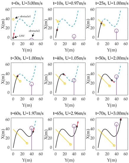
Figure 6.
Time diagram of USV path following and dynamic obstacle avoidance.
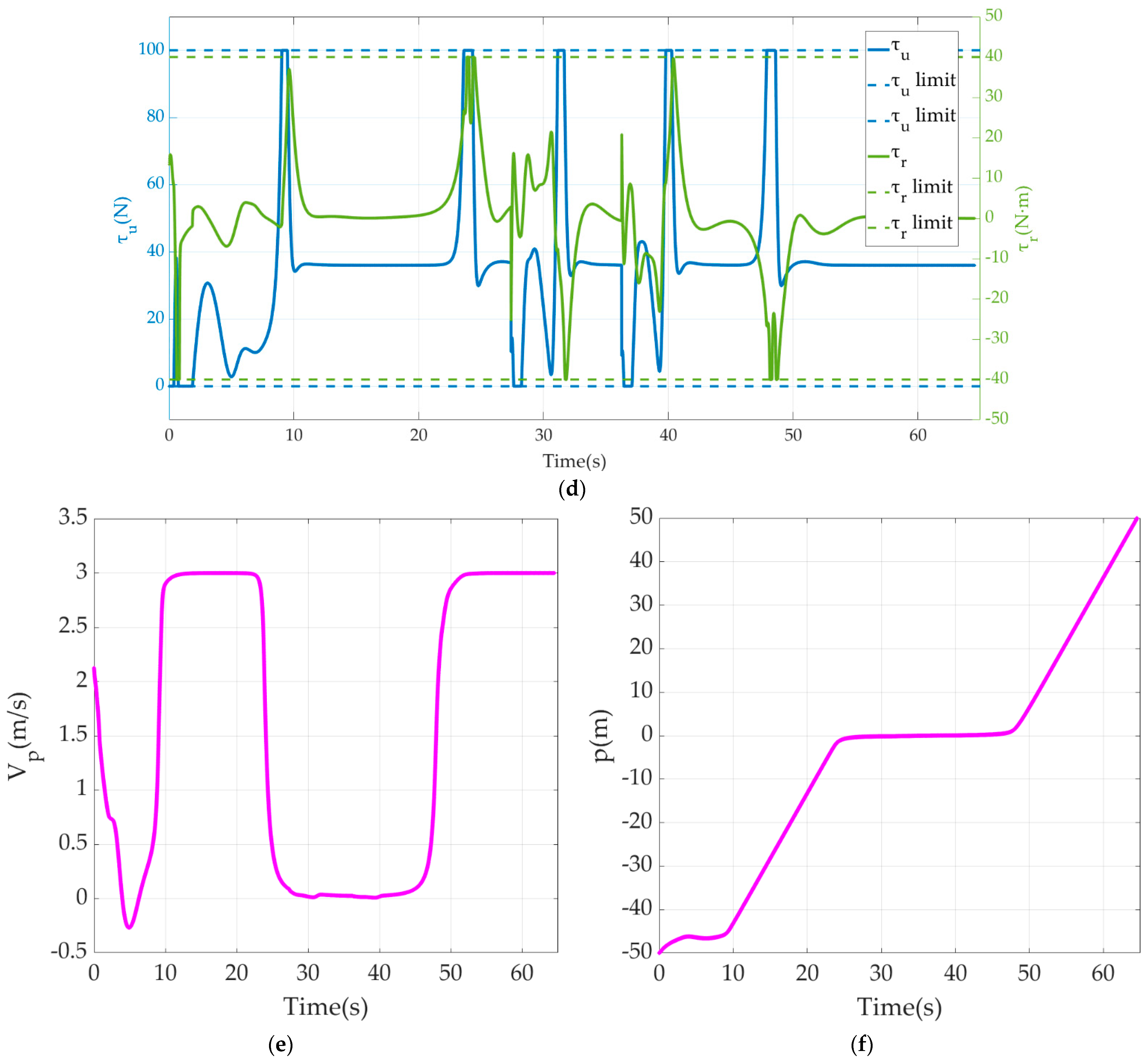
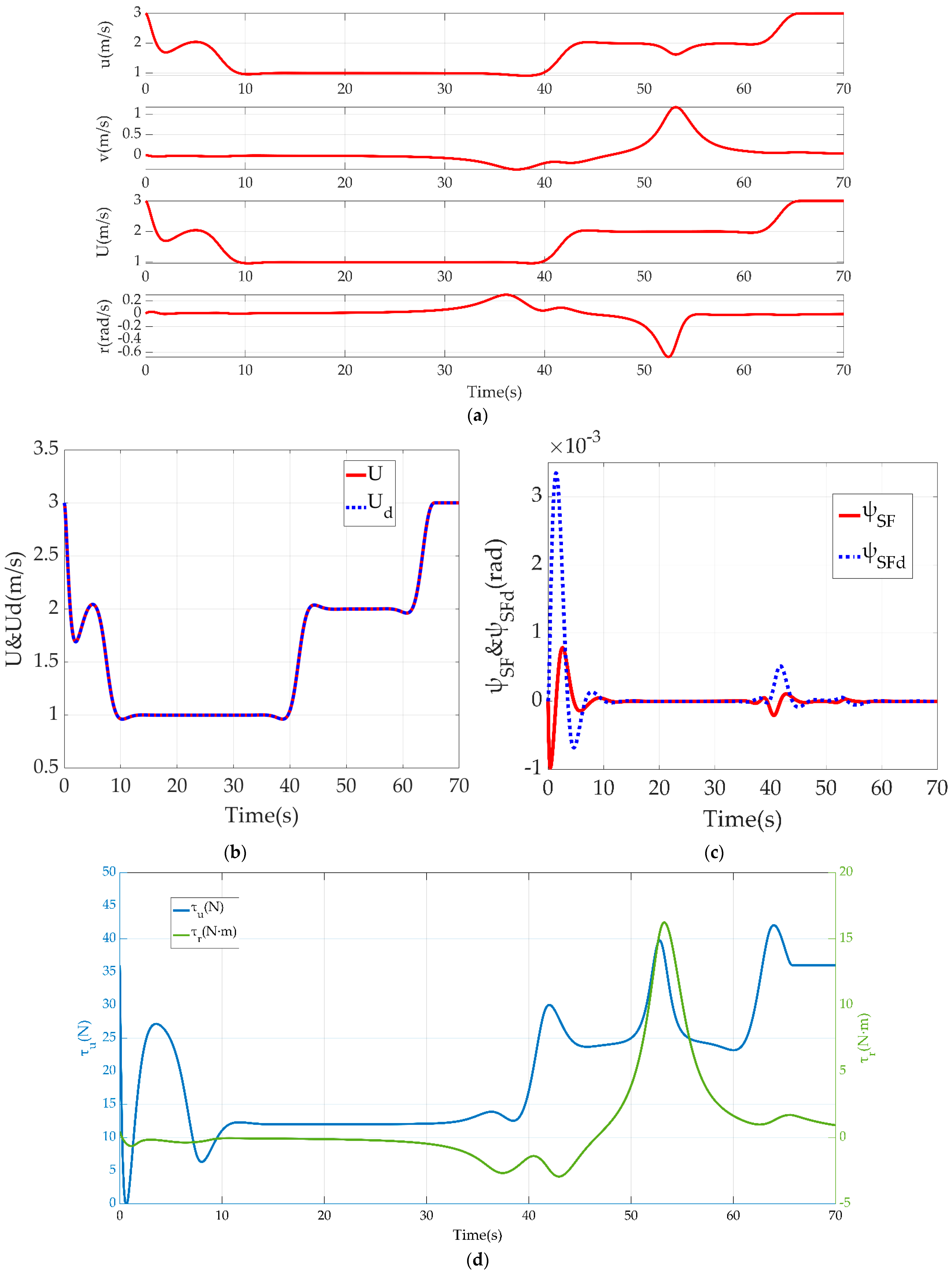
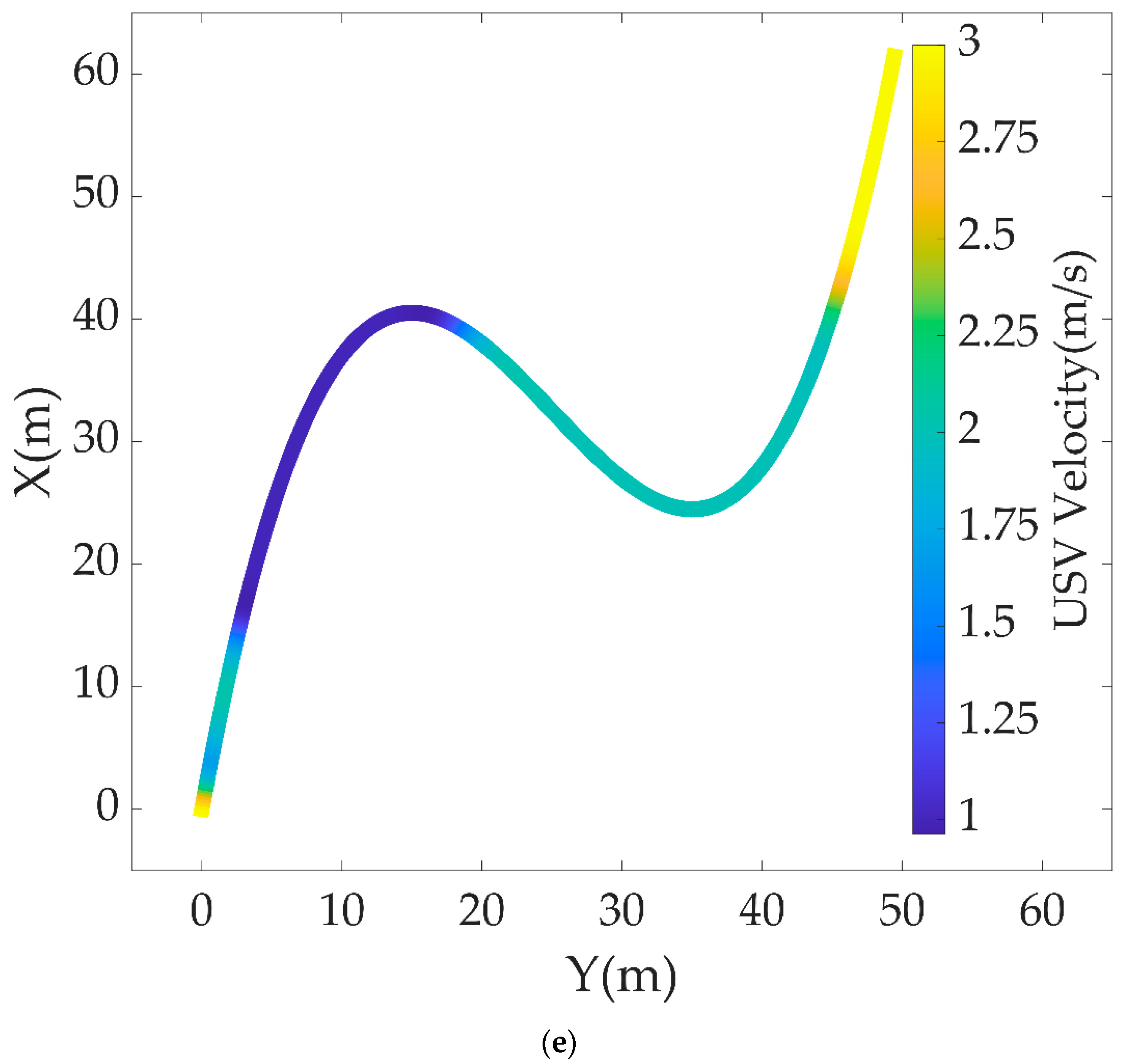
Figure 7 shows a series of data related to the underlying motion control of the USV in this obstacles avoidance scenario. Figure 7a records the rate of motion on 3-DOF of surge, sway and yaw, and the real moving velocity. Figure 7b,c shows the control effect towards set values by an outer loop of RVC and NBCC, respectively. Figure 7d is the time curve of USV thrust and torque output. Figure 7e reflects the actual velocity at different positions on the USV trajectory, ranging from 1 m/s to 3 m/s. The lower the colour temperature is, the higher the USV resultant velocity is.
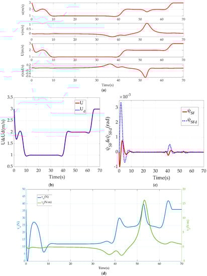

Figure 7.
Results of USV underlying motion control: (a) USV 3-DOF motion data; (b) Tracking effect of RVC on expected velocity; (c) Tracking effect of NBCC on LOS guidance law; (d) Thrust and torque output; (e) USV resultant velocity on its trajectory.
7. Discussion
From the simulation results of Section 6.1, this paper puts forward the velocity control of USV based on its position and attitude, which enables USV to correct the initial position deviation through a smaller steering radius to reduce the path loss. USV can also correct the derailment caused by the sudden disturbance from the outside environment with a smaller space loss due to such a velocity planning scheme. Furthermore, such a scheme will not produce adverse results of overshoot or even oscillation concerning the same LOS forward-looking distance parameter, which will greatly improve the smoothness and accuracy of transition in correction. Figure 3 shows the convergence effect of the USV motion control strategy and path following from the perspective of the {SF} frame. An analysis of the results of USV underlying motion control shows that the moving velocity and course both track the setpoints and overcome the disturbance remarkably. In particular, a comparison of the data in the 20–50 s time range of Figure 4a–c shows that when USV is derailing (caused by the too-small path curvature at around 24 s and 48 s, disturbance’s occurrence at around 28 s and disturbance’s disappearance at around 36 s), subject to velocity control and the ship’s maneuvering characteristics, USV’s performance is reflected in the decrease of surge velocity and increase of sway velocity, while the resultant velocity decreases and a certain drift angle occurs. Vividly speaking, USV completes the steering process in a “drifting” way with velocity deceleration which is more consistent with reality. This is an effective way to reduce the offset and complete the derailment correction as soon as possible, improving the maneuverability and flexibility of the USV. When USV succeeds to move to the preset path, the velocity set value will be increased to the expected patrol velocity, which can also be customized by the specific operation task. In addition, the output of thrust and torque is saturated, but mainly at the moment of sharp steering and acceleration, which is related to the power exponent form of Equation (23) used in variable velocity correction. Finally, the velocity and position data of reference points are consistent with USV velocity and position, which conforms to the essence of path reference points being used as the base for SF coordinate system construction, and the significance of converging USV’s path following error system by introducing such virtual control variable.
In Section 6.2, we first calculated and plotted the ST graph of a relationship between preset path curve and dynamic obstacle encroachment, which means that the USV cannot appear at the corresponding path distance at the corresponding time, otherwise a collision will be inevitable. The ST graph transfers the complex collision problem in the scale of time and space to the path searching problem in a 2-D image. The use of DP and QP optimization algorithms finally gives a continuous and smooth velocity planning including velocity, acceleration and jerk with respect to the constraints and costs from the actual situation. This ensures the smoothness of USV velocity variation, the continuity of motion trajectory curvature, and the smoothness of actuator outputs. The continuity of motion trajectory curvature means that the preset path in this planning is traceable for the USV because the USV cannot move horizontally or stop. And a mutational curvature of the desired path means that the USV will have a transition process of temporary deviation from the path. Although it is possible to return to the desired path eventually, such temporary deviation should be avoided in scenarios where moving obstacles may be all around. The greatest value of this time-for-space method can be seen from the time diagram of scenario simulation, that is, the USV can evade obstacles by adjusting its velocity but not breaking away from the preset path. The logic behind it lies in the fact that the preset path is usually well planned for many factors, e.g., task requirement, channel limits, navigation rules and so on. In other words, it is very likely to encounter new troubles if a local path is created for obstacle avoidance. Therefore, it is better to let the USV follow the preset path as close as possible, and realizing obstacle avoidance through velocity planning deserves a higher priority than making local path planning to generate a new route away from the preset path, which is the conventional method that most works adopt. Of course, when velocity planning fails, which means that there is no solution from dynamic programming on the ST graph, USV cannot but resort to local planning to avoid an incoming collision. From the perspective of the underlying motion control data, the USV has achieved the tracking of the expected velocity and heading precisely, which is also the basis for applying velocity planning. Figure 7e is a colourmap that directly shows the actual velocity of the USV moving at different positions of its trajectory according to velocity planning for obstacle avoidance.
8. Conclusions
In this paper, the motion control and path-following problems of a USV and the application scenario expansion based on velocity planning are studied and discussed strictly according to the research ideas of control theory and the engineering application field. The process includes mathematical modelling, controller design, stability proof, scenario optimization and simulation verification. The simulation results of USV in two scenarios verify the effectiveness and reliability of the motion control strategy and the path following algorithm proposed in this study. Secondly, the simulation results show that both velocity planning strategies perform well in derailment and obstacle avoidance scenarios. Through the detailed display and analysis of the result data, the feasibility and practicability of the research and design ideas in this paper to solve the problems of the USV path following control, derailment correction and dynamic obstacle avoidance are fully proved, which is also the main contribution and value of this study. Some details not involved in the whole process, such as model parameter perturbation, actuator saturations, obstacle perception and judgement, real ship identification and test, have formed the subject direction for follow-up in-depth research which will motivate the scientific research and promotion of autonomous unmanned system technology together with this study.
Author Contributions
Conceptualization, Z.F. and J.L.; methodology, Z.F. and Y.L.; software, Z.F.; validation, Z.F. and Z.P.; formal analysis, Z.F.; investigation, Z.F. and W.C.; resources, Z.P. and J.L.; data curation, Z.F. and Z.P.; writing—original draft preparation, Z.F. and W.C.; writing—review and editing, Z.F.; visualization, Z.F.; supervision, Y.L. and J.L.; project administration, Z.F. and J.L. All authors have read and agreed to the published version of the manuscript.
Funding
This research received no external funding.
Institutional Review Board Statement
Not applicable.
Informed Consent Statement
Not applicable.
Data Availability Statement
The USV mathematical model used in this article for numerical simulation comes from a small ship model developed by K.D. Do & J. Pan and its parameters are calculated by VERES [29].
Acknowledgments
Thanks for research conditions provided by Institute of marine structures and naval architectures, Ocean College, Zhejiang University and technical sharing from unmanned system academics and hobbyists.
Conflicts of Interest
The authors declare that they have no conflict of interest.
Appendix A
When applying Lyapunov Direct Method in RVC design, the desired resultant velocity is marked as . The velocity error and its derivative are written as and respectively:
Construct control-Lyapunov function and its derivative :
Obviously, is positive definite. According to the Lyapunov stability method, is supposed to be negative definite in order to make converge to zero. Then it can be designed:
where the positive parameter is the controller gain.
Substituting the Equation (9) into Equation (A3) can obtain the final control law for USV resultant velocity:
Appendix B
According to the design idea of the backstepping method, the course tracking error is first written as , and its derivative is written as :
Construct control-Lyapunov function and its derivative :
Obviously, is positive definite. According to the Lyapunov stability method, is supposed to be negative definite in order to make converge to zero. Then it can be designed:
where the positive parameter is the controller gain of the first layer. is introduced as a new desired value with respect to angular velocity for course changing. Therefore, an error function of is introduced, denoted as :
Differentiating and combining Equations (A5) and (A7) leads to:
Then construct the control-Lyapunov function and its derivate :
Obviously, is positive definite. According to the Lyapunov stability method, is supposed to be negative definite in order to make both and converge to zero. Then it can be designed:
where the positive parameter is the controller gain of the second layer.
Substitute the error Equations (A5), (A8) and (A9) defined above, and combine the USV kinetic model (1) with the error Equation (5) of path following under the {SF} frame. The USV course control law can be obtained at last:
References
- Liu, Z.; Zhang, Y.; Yu, X.; Yuan, C. Unmanned surface vehicles: An overview of developments and challenges. Annu. Rev. Control 2016, 41, 71–93. [Google Scholar] [CrossRef]
- Jorge, V.A.; Granada, R.; Maidana, R.G.; Jurak, D.A.; Heck, G.; Negreiros, A.P.; Amory, A.M. A survey on unmanned surface vehicles for disaster robotics: Main challenges and directions. Sensors 2019, 19, 702. [Google Scholar] [CrossRef] [PubMed] [Green Version]
- Zhou, C.; Gu, S.; Wen, Y.; Du, Z.; Xiao, C.; Huang, L.; Zhu, M. The review unmanned surface vehicle path planning: Based on multi-modality constraint. Ocean Eng. 2020, 200, 107043. [Google Scholar] [CrossRef]
- Tran, N.H.; Pham, Q.H.; Lee, J.H.; Choi, H.S. VIAM-USV2000: An Unmanned Surface Vessel with Novel Autonomous Capabilities in Confined Riverine Environments. Machines 2021, 9, 133. [Google Scholar] [CrossRef]
- Mu, D.; Wang, G.; Fan, Y.; Zhao, Y. Modeling and Identification of Podded Propulsion Unmanned Surface Vehicle and Its Course Control Research. Math. Probl. Eng. 2017, 2017, 1–13. [Google Scholar] [CrossRef]
- Ren, R.Y.; Zou, Z.J.; Wang, Y.D.; Wang, X.G. Adaptive Nomoto model used in the path following problem of ships. J. Mar. Sci. Technol. 2018, 23, 888–898. [Google Scholar] [CrossRef]
- Fossen, T.I. Marine Control Systems; Norwegian University of Science and Technology: Trondheim, Norway, 2002; pp. 50–113. [Google Scholar]
- Fossen, T.I. Guidance and Control of Ocean Vehicles; Wiley: New York, NY, USA, 1994; pp. 48–54. [Google Scholar]
- Wu, W.; Peng, Z.; Wang, D.; Liu, L.; Han, Q.L. Network-Based Line-of-Sight Path Tracking of Underactuated Unmanned Surface Vehicles With Experiment Results. IEEE Trans. Cybern. 2021, 99, 1–11. [Google Scholar] [CrossRef]
- Wen, Y.; Tao, W.; Zhu, M.; Zhou, J.; Xiao, C. Characteristic model-based path following controller design for the unmanned surface vessel. Appl. Ocean Res. 2020, 101, 102293. [Google Scholar] [CrossRef]
- Cao, H.; Xu, R.; Zhao, S.; Li, M.; Song, X.; Dai, H. Robust trajectory tracking for fully-input-bounded actuated unmanned surface vessel with stochastic disturbances: An approach by the homogeneous nonlinear extended state observer and dynamic surface control. Ocean. Eng. 2022, 243, 110113. [Google Scholar] [CrossRef]
- Liu, L.; Liu, Z.; Zhang, J. LMI-Based Model Predictive Control for Underactuated Surface Vessels with Input Constraints. Abstr. Appl. Anal. 2014, 2014, 1–9. [Google Scholar] [CrossRef]
- Jin, J.C.; Zhang, J.; Liu, D.Q. Design and Verification of Heading and Velocity Coupled Nonlinear Controller for Unmanned Surface Vehicle. Sensors 2018, 18, 3427. [Google Scholar] [CrossRef] [PubMed] [Green Version]
- González-Prieto, J.A.; Pérez-Collazo, C.; Singh, Y. Adaptive Integral Sliding Mode Based Course Keeping Control of Unmanned Surface Vehicle. J. Mar. Sci. Eng. 2022, 10, 68. [Google Scholar] [CrossRef]
- Su, Y.; Wan, L.; Zhang, D.; Huang, F. An improved adaptive integral line-of-sight guidance law for unmanned surface vehicles with uncertainties. Appl. Ocean. Res. 2021, 108, 102488. [Google Scholar] [CrossRef]
- Li, L.; Pei, Z.; Jin, J.; Dai, Y. Control of Unmanned Surface Vehicle Along the Desired Trajectory Using Improved Line of Sight and Estimated Sideslip Angle. Pol. Marit. Res. 2021, 28, 18–26. [Google Scholar] [CrossRef]
- Yu, Y.; Guo, C.; Li, T. Finite-time LOS Path Following of Unmanned Surface Vessels with Time-varying Sideslip Angles and Input Saturation. IEEE/ASME Trans. Mechatron. 2021, 27, 463–474. [Google Scholar] [CrossRef]
- Liu, T.; Dong, Z.; Du, H.; Song, L.; Mao, Y. Path Following Control of the Underactuated USV Based On the Improved Line-of-Sight Guidance Algorithm. Pol. Marit. Res. 2017, 24, 3–11. [Google Scholar] [CrossRef] [Green Version]
- Mu, D.; Wang, G.; Fan, Y.; Bai, Y.; Zhao, Y. Fuzzy-Based Optimal Adaptive Line-of-Sight Path Following for Underactuated Unmanned Surface Vehicle with Uncertainties and Time-Varying Disturbances. Math. Probl. Eng. 2018, 2018, 1–12. [Google Scholar] [CrossRef] [Green Version]
- Song, A.L.; Su, B.Y.; Dong, C.Z.; Shen, D.W.; Xiang, E.Z.; Mao, F.P. A two-level dynamic obstacle avoidance algorithm for unmanned surface vehicles. Ocean. Eng. 2018, 170, 351–360. [Google Scholar] [CrossRef]
- Ren, J.; Zhang, J.; Cui, Y. Autonomous Obstacle Avoidance Algorithm for Unmanned Surface Vehicles Based on an Improved Velocity Obstacle Method. ISPRS Int. J. Geo-Inf. 2021, 10, 618. [Google Scholar] [CrossRef]
- Liu, X.; Li, Y.; Zhang, J.; Zheng, J.; Yang, C. Self-Adaptive Dynamic Obstacle Avoidance and Path Planning for USV Under Complex Maritime Environment. IEEE Access 2019, 7, 114945–114954. [Google Scholar] [CrossRef]
- Xia, G.; Han, Z.; Zhao, B.; Wang, X. Local Path Planning for Unmanned Surface Vehicle Collision Avoidance Based on Modified Quantum Particle Swarm Optimization. Complexity 2020, 2020, 1–15. [Google Scholar] [CrossRef]
- Chen, Y.; Bai, G.; Zhan, Y.; Hu, X.; Liu, J. Path Planning and Obstacle Avoiding of the USV Based on Improved ACO-APF Hybrid Algorithm With Adaptive Early-Warning. IEEE Access 2021, 9, 40728–40742. [Google Scholar] [CrossRef]
- Xia, G.; Han, Z.; Zhao, B.; Wang, X. Unmanned Surface Vehicle Collision Avoidance Trajectory Planning in an Uncertain Environment. IEEE Access 2020, 8, 207844–207857. [Google Scholar] [CrossRef]
- Fossen, T.I. Handbook of Marine Craft Hydrodynamics and Motion Control; John Wiley & Sons: Hoboken, NJ, USA, 2011; pp. 133–140. [Google Scholar]
- Xiao, L.; Jouffroy, J. Modeling and Nonlinear Heading Control of Sailing Yachts. IEEE J. Ocean. Eng. 2013, 39, 256–268. [Google Scholar] [CrossRef]
- Li, D.; Du, L. AUV Trajectory Tracking Models and Control Strategies: A Review. J. Mar. Sci. Eng. 2021, 9, 1020. [Google Scholar] [CrossRef]
- Do, K.D.; Pan, J. Robust path-following of underactuated ships: Theory and experiments on a model ship. Ocean. Eng. 2006, 33, 1354–1372. [Google Scholar] [CrossRef]
Publisher’s Note: MDPI stays neutral with regard to jurisdictional claims in published maps and institutional affiliations. |
© 2022 by the authors. Licensee MDPI, Basel, Switzerland. This article is an open access article distributed under the terms and conditions of the Creative Commons Attribution (CC BY) license (https://creativecommons.org/licenses/by/4.0/).