An Artificial Neural Network Approach for Solving Inverse Kinematics Problem for an Anthropomorphic Manipulator of Robot SAR-401

Abstract

The paper proposes a new design of an artificial neural network for solving the inverse kinematics problem of the anthropomorphic manipulator of robot SAR-401. To build a neural network (NN), two sets were used as input data: generalized coordinates of the manipulator and elements of a homogeneous transformation matrix obtained by solving a direct kinematics problem based on the Denavi–Hartenberg notation. According to the simulation results, the NN based on the homogeneous transformation matrix showed the best accuracy. However, the accuracy was still insufficient. To increase the accuracy, a new NN design was proposed. It consists of adding a so-called “correctional” NN, the input of which is fed the same elements of the homogeneous transformation matrix and additionally the output of the first NN. The proposed design based on the correctional NN allowed the accuracy to increase two times. The application of the developed NN approach was carried out on a computer model of the manipulator in MATLAB, on the SAR-401 robot simulator, as well as on the robot itself.

1. Introduction

Modern manipulators that allow solving high-precision technological tasks are kinematically redundant. They have at least 6 degree of freedom (DOF) which provides sufficient mobility and flexibility to solve complex tasks. An obvious and natural approach to a control design of anthropomorphic robot manipulators is an approach based on solving the inverse kinematics problem (IKP).

The complexity of the IKP of anthropomorphic manipulators arises from the nonlinear equations that arise between the Cartesian space and the joint space [1]. Solving the IKP is one of the important problems, which requires solving a system of nonlinear differential equations and calculating the pseudoinverse Jacobi matrix [2]. This problem is computationally complex [3]. The use of conventional numerical methods to solve it is time-consuming. They often have a singularity [4]. Considering that neural networks (NN) are designed to solve nonlinear equations, some papers [4,5,6,7,8] propose an approach to the control design of anthropomorphic manipulators based on the NN approach to reduce the computational complexity of control design.

The main direction of a NN design for solving the IKP is related to the influence of structural parameters (the number of hidden layers and the number of neurons in each hidden layer), iteration steps, and a training dataset on the performance of the IKP solution approximation [9,10]. At the same time, it is not recommended to complicate a NN configuration, because this leads to a significant increase in the number of iterations to achieve the required learning goal [11]. The training dataset for a NN design is obtained either by solving a direct kinematics problem (DKP) or by experiments.

Some robots with anthropomorphic manipulators have copy-type master device that allow forming a training dataset without solving the DKP. Note that this method has some disadvantages: limitations of the experimental equipment in terms of the accuracy of the measured data and more time spent collecting the training dataset.

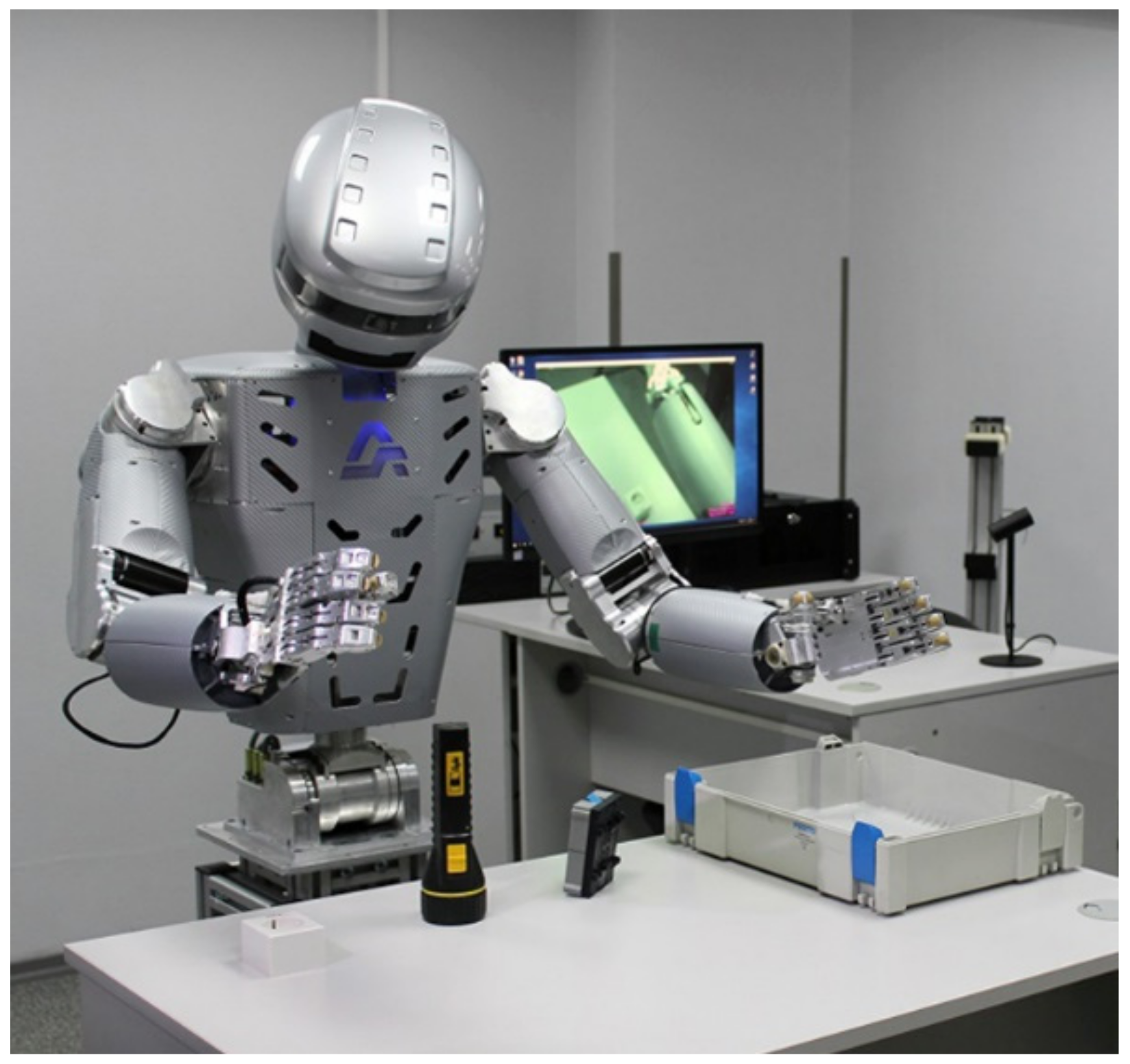
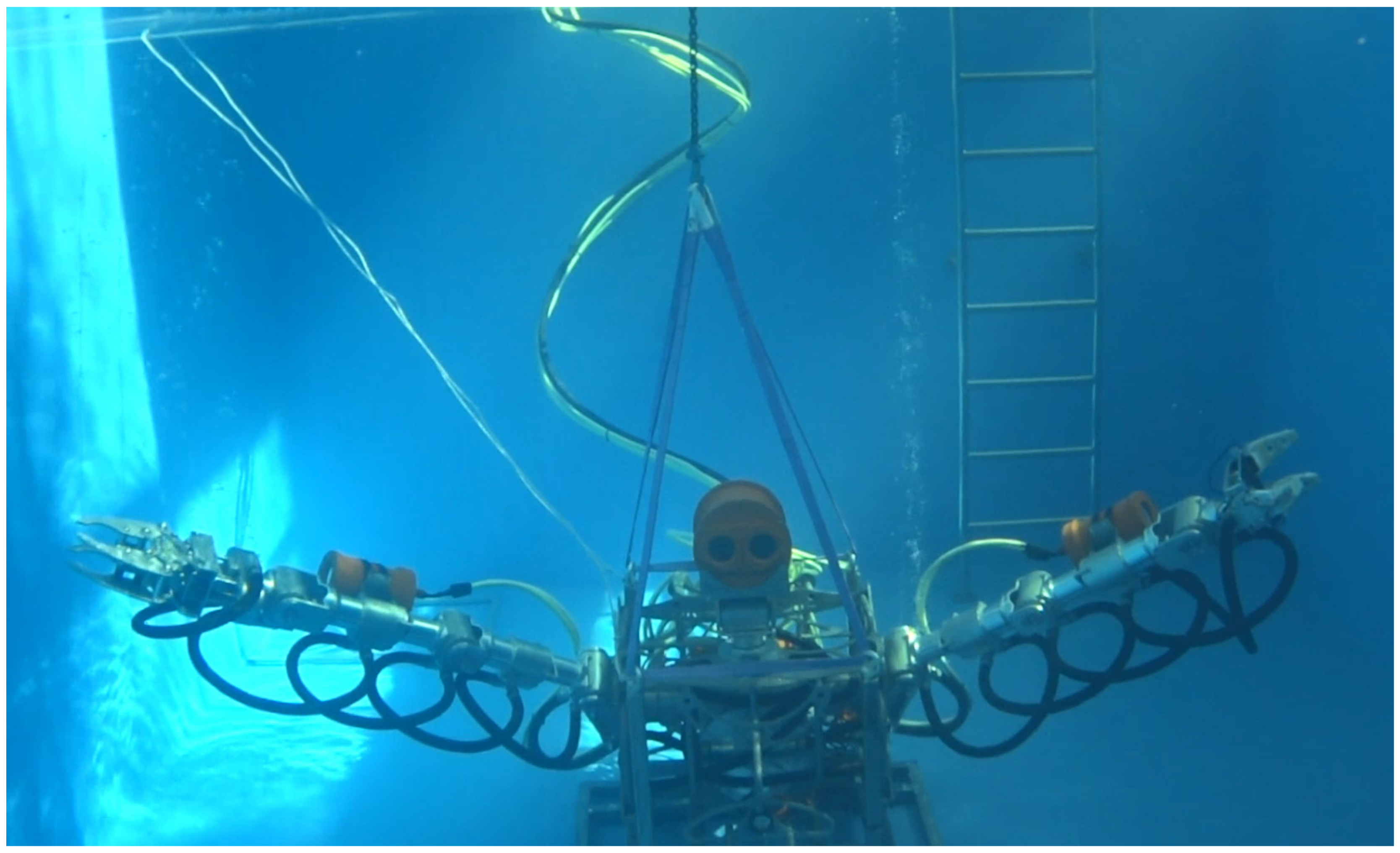
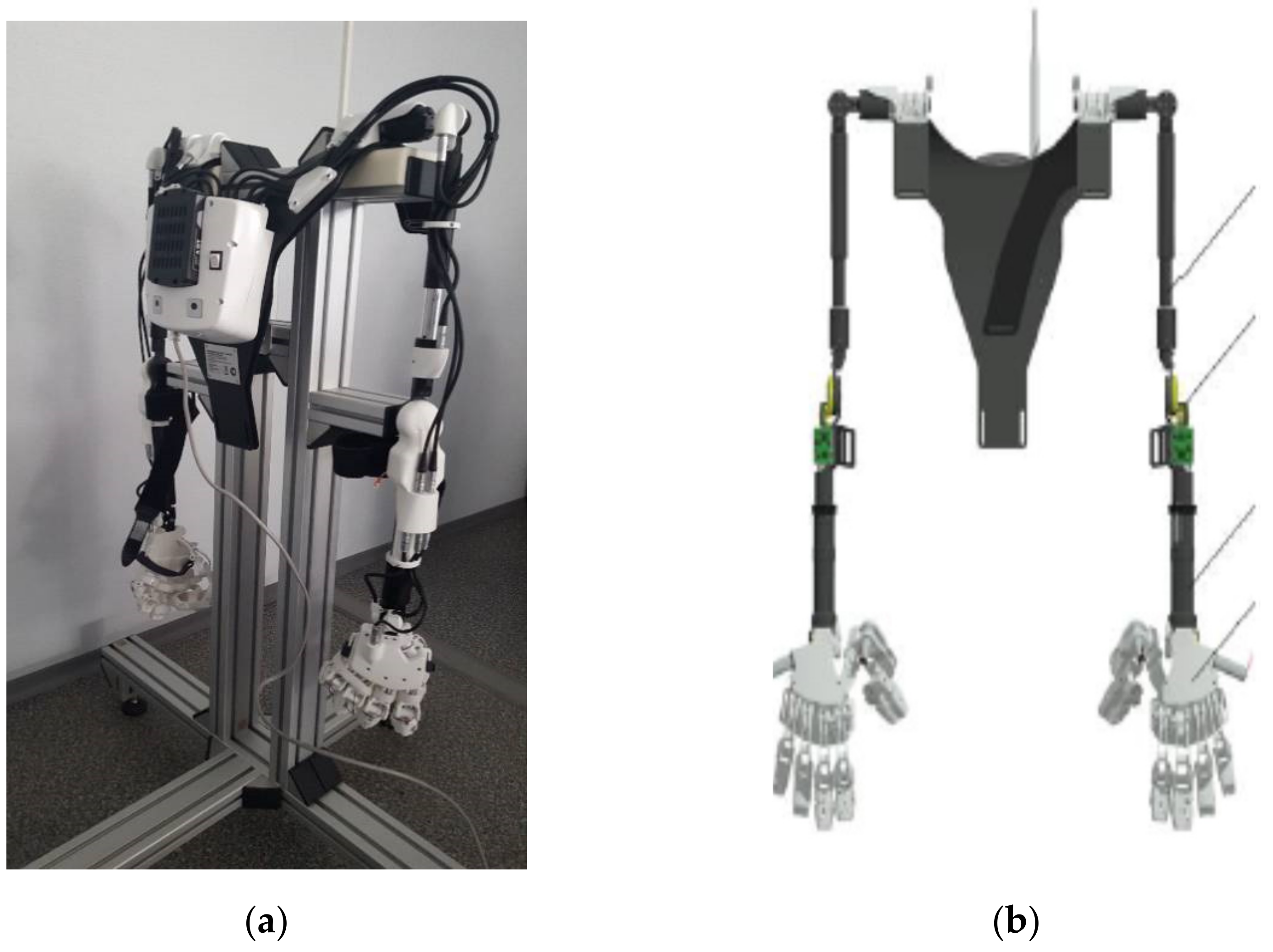
As an example of a robot with a copy-type master device, one can indicate the robot SAR-401 (see Figure 1) [12,13] and the underwater robot “Ichthyandr” (see Figure 2) [14,15]. Both robots are produced by the company “Android Technology”. The manipulators of these robots have 7-DOF. Copy-type master device for robots is shown in Figure 3.

Figure 1. Robot SAR-401.

Figure 2. The underwater robot “Ichthyandr”.

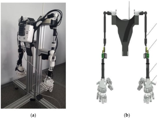
Figure 3. Copy-type master devices. (a) for the robot SAR-401; (b) for underwater robot “Ichthyandr”.

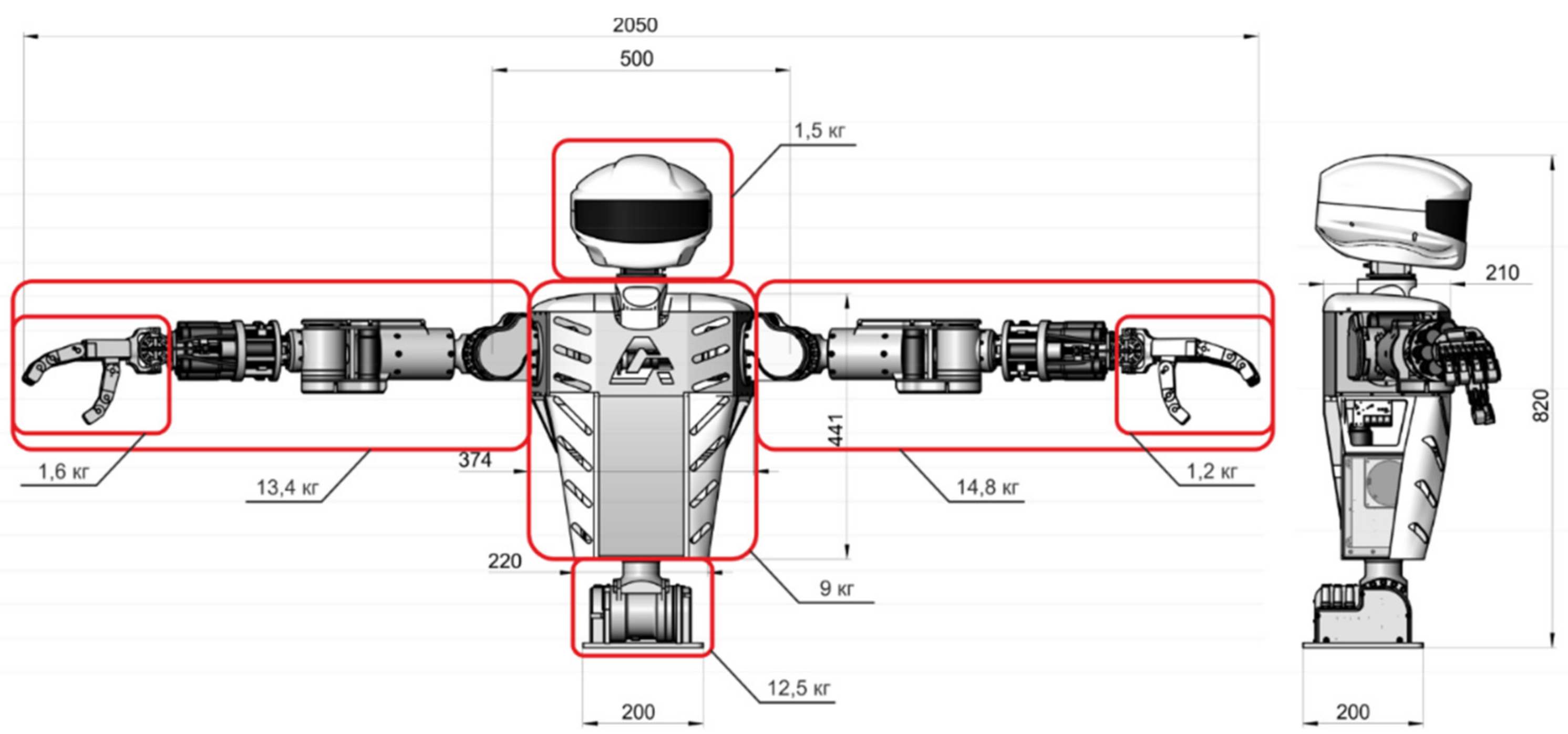
In this paper, the robot SAR-401 will be considered as an object for further research. The robot SAR-401 without a stand is shown in Figure 4. Let us briefly summarize the main characteristics of the robot SAR-401.

Figure 4. The torso anthropomorphic robot, model SAR-401 (without stand).

The general characteristics of the robot SAR-401: weight—70 kg; height—820 mm; a span of manipulators—2050 mm; number of video cameras—2 (stereo vision mode).

The main advantages of the robot SAR-401 are the performance of technological operations with efficiency comparable to human actions; force-torque feedback for the operator; the possibility of using a tool used by an operator; work in automatic and copying mode with copy-type master device.

As already noted, there are a large number of papers describing the NN design for solving the IKP for anthropomorphic manipulators. At the same time, there is no one universal solution for all types of robots.

This paper describes the design of the NN for solving the IKP of anthropomorphic manipulators of the robot SAR-401. The proposed design is based on the use of the so-called “correctional” structure of the NN and the special choice of the structure of the input dataset.

2. Materials and Methods

2.1. Kinematics Analysis of the Robot SAR-401

The generalized coordinates $q_i$ of the manipulator obtaining from the given coordinates $x, y, z$ and Euler angles $\varphi , \theta , \gamma$ of the end-effector can be used as a training dataset. The end-effector coordinates are defined in the Cartesian coordinate system relative to the base of the robot. As mentioned above, the training dataset can be obtained using the copy-type master device. Additionally, knowing the exact characteristics of the robot, we can obtain the training dataset as a result of solving the DKP.

To solve the DKP we use a kinematic diagram of the anthropomorphic manipulators of the robot SAR-401 (Figure 5) and the notation and methodology of Denavit–Hartenberg [16]. We will consider the left manipulator of the robot. Since this manipulator has only rotational joints, the relative location of neighboring links will be determined by the angular variable ${\theta }_i$.

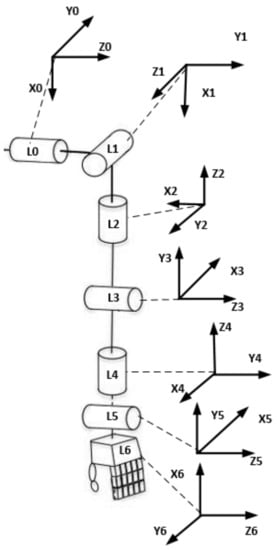
Figure 5. The kinematic diagram of the robot SAR-401 left manipulator.

The Denavit–Hartenberg parameters for the left manipulator of the robot SAR-401 are shown in Table 1.

Table 1. DH parameters for the left manipulator of the robot SAR-401.

Link, i	${\mathit{A}}_{\mathit{i}},\mathbf{m}$	${\mathit{\alpha }}_{\mathit{i}},\mathbf{Rad}$	${\mathit{d}}_{\mathit{i}},\mathbf{m}$	${\mathit{\theta }}_{\mathit{i}}, \mathbf{Rad}$
1	0	π/2	0	${\theta }_i$
2	0	π/2	0	${\theta }_i-\pi /2$
3	0	π/2	−0.3	${\theta }_i-\pi$
4	0	π/2	0	${\theta }_i+\pi$
5	0	π/2	−0.3	${\theta }_i+\pi$
6	−0.24	0	0	${\theta }_i+\pi /2$

In Table 1, the following notations are accepted: $A_i$ is the distance between the $Z_{i-1}$ and $Z_i$ axes along the $X_i$ axis, ${\alpha }_i$ is the angle from the $Z_{i-1}$ axis to the $Z_i$ axis about the $X_i$ axis, $d_i$ is the distance from the origin of the frame $i-1$ to the $X_i$ axis along the $Z_{i-1}$ axis, ${\theta }_i$ are generalized coordinates (the angles of rotation of joints). The parameters ${\theta }_i, i=\overline{1, 6}$ are variables and are initially 0.

For the right manipulator the Denavit–Hartenberg parameters are identical.

The limits on the movements of the servo drive of the joints of the robot SAR-401 manipulators are given in Table 2. The numbering of the servo drives is shown in Figure 5.

Table 2. Manipulator servo drives limits.

Servo	Left Manipulator		Right Manipulator
	Min	Max	Min	Max
0	−90°	0°	−90°	0°
1	0°	105°	−105°	0°
2	−40°	40°	−40°	40°
3	−110°	5°	−110°	5°
4	−40°	40°	−40°	40°
5	−10°	10°	−10°	10°

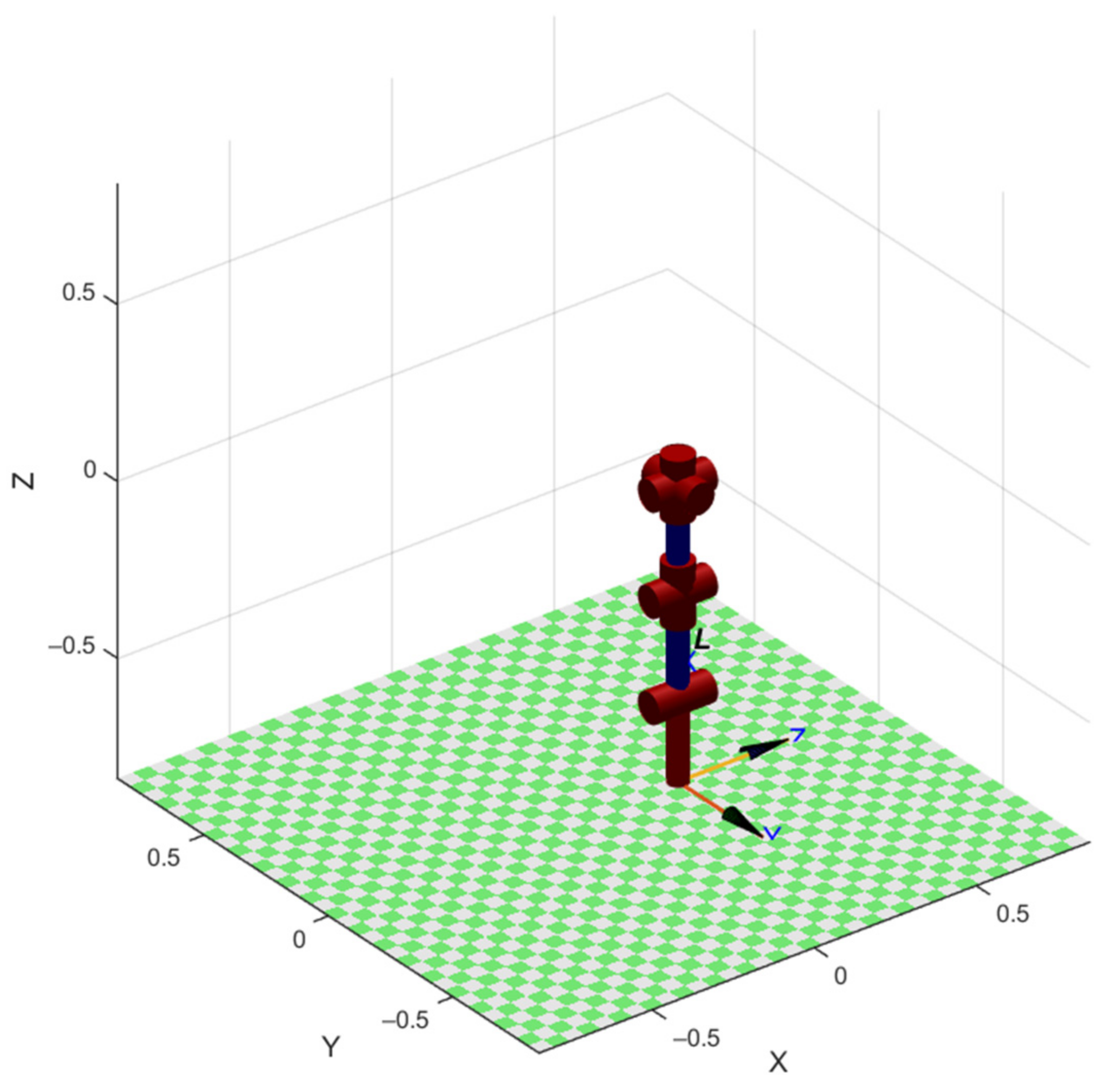
To build a computer model of the manipulator kinematics, we will use the RoboticsToolbox of MATLAB [17]. The values of parameters $A_i$, ${\alpha }_i$, and $d_i$ are selected from Table 1. The parameter ${\theta }_i$ describes the initial position of the manipulator.

A visual representation of the computer model of the initial position of the robot SAR-401 left manipulator is shown in Figure 6.

Figure 6. The computer model of the initial position of the robot SAR-401 left manipulator.

2.2. Training Dataset for Neural Network

At the initial stage of designing the NN, we must choose a training dataset. The input dataset must be associated with the coordinates $x, y, z$ and Euler angles $\varphi , \theta , \gamma$ of the manipulator’s end-effector.

The training dataset using the copy-type master device consists of the random location of the manipulators and corresponding coordinates $x, y, z$ and Euler angles $\varphi , \theta , \gamma$ of the end-effector. The position of the manipulator changes by operator until a sufficient amount of data is collected.

To prepare the training dataset for the NN using a copy-type master device, we randomly select the possible positions of the manipulator in different places of its working area. The obtained data will be saved as a vector $Y=[q_1 q_2 q_3 \dots q_6]$, where $q_i, i=\overline{1, 6}$ is the generalized coordinate of the i-th joint.

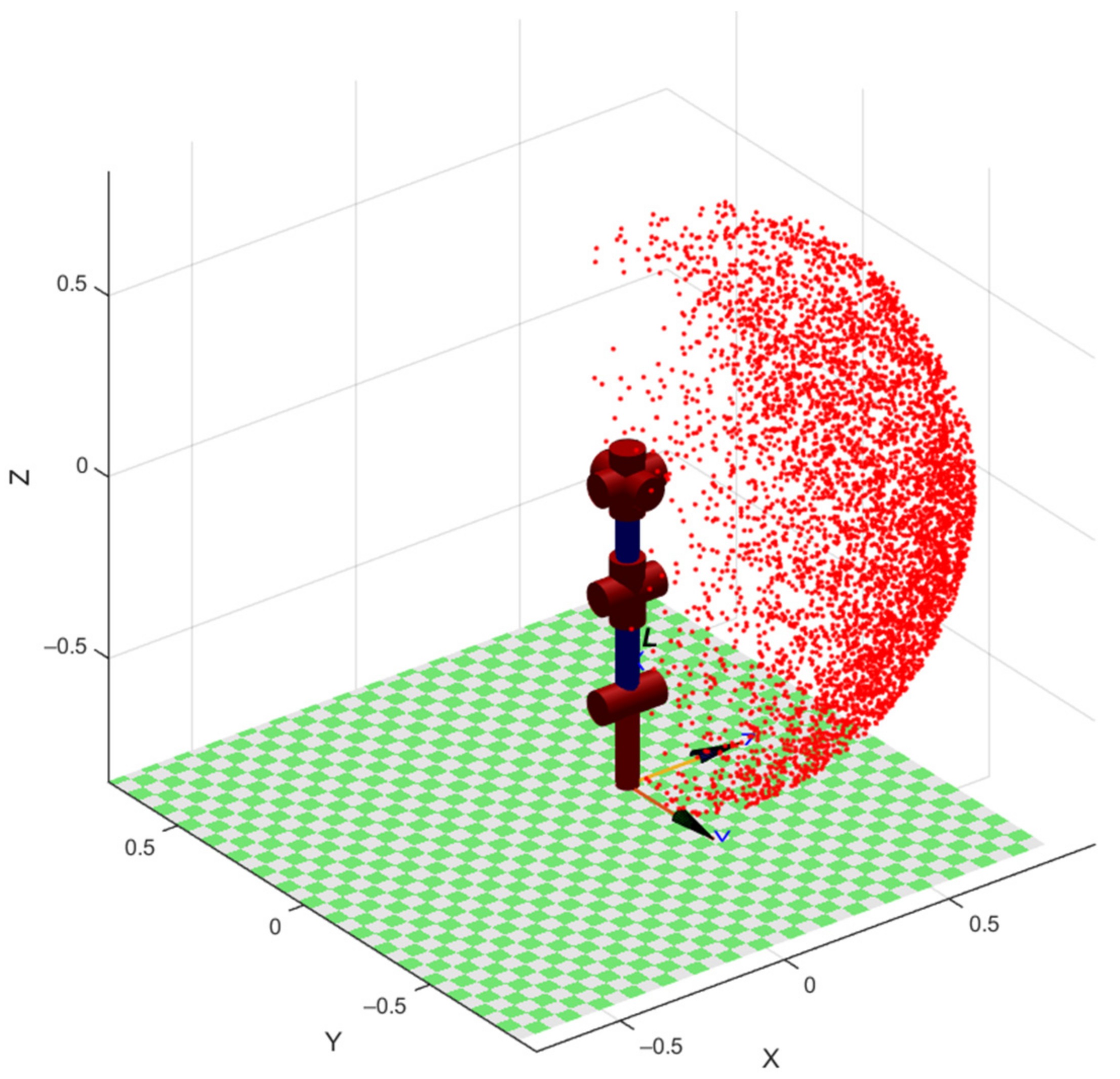
To prepare the training dataset using the solution of the DKP for each position of the manipulator, we find the coordinates of the end effector. Figure 7, as an example, shows the result of solving the forward kinematics problem for 30,000 randomly generated positions of the manipulator.

Figure 7. The solution of the forward kinematics problem for 30,000 random positions.

When solving the DKP, two coordinate systems are considered: the initial one, associated with the base joint $x_0, y_0, z_0$, and the final one, associated with the end-effector of the manipulator $x_n, y_n, z_n$.

Extended position vectors ${\widehat{X}}_0={\left[\begin{array}{cccc}{x}_0& y_0& z_0& 1\end{array}\right]}^T$ and ${\widehat{X}}_n={\left[\begin{array}{cccc}{x}_n& y_n& z_n& 1\end{array}\right]}^T$, for the specified coordinate systems, are related by the formula

$${\widehat{X}}_0=T_n^0{\widehat{X}}_n,$$

(1)

where $T_n^0=\left[\begin{array}{cc}{R}_{3x3}& p_{3x1}\\ f_{1x3}& t\end{array}\right]$ is a 4 × 4 matrix of a homogeneous transformation that carries information about the translation (vector $p_{3x1}$) and the rotation of one coordinate system relative to another (matrix $R_{3x3}$), $f_{1x3}$ is a 1 × 3 vector that specifies the perspective transformation, $t$ is a global scaling factor. In our case, $f_{1x3}=[0 0 0]$, $t=1$.

Now, for each joint, we can define the homogeneous transformation matrix $T_i$, which specifies a sequence of transformations according to the Denavit–Hartenberg notation

$$T_i=T_{z d_i}{T}_{z {\theta }_i}{T}_{x A_i}{T}_{x {\alpha }_i}=\left[\begin{array}{cc}I& p_{d_i}\\ 0& 1\end{array}\right]\left[\begin{array}{cc}{R}_{z {\theta }_i}& 0\\ 0& 1\end{array}\right]\left[\begin{array}{cc}I& p_{A_i}\\ 0& 1\end{array}\right]\left[\begin{array}{cc}{R}_{x {\alpha }_i}& 0\\ 0& 1\end{array}\right].$$

(2)

$$\begin{array}{l}{T}_i=\\ =\left[\begin{array}{cccc}1& 0& 0& 0\\ 0& 1& 0& 0\\ 0& 0& 1& d_i\\ 0& 0& 0& 1\end{array}\right]\left[\begin{array}{cccc}\cos {\theta }_i& -\sin {\theta }_i& 0& 0\\ \sin {\theta }_i& \cos {\theta }_i& 0& 0\\ 0& 0& 1& 0\\ 0& 0& 0& 1\end{array}\right]\left[\begin{array}{cccc}1& 0& 0& A_i\\ 0& 1& 0& 0\\ 0& 0& 1& 0\\ 0& 0& 0& 1\end{array}\right]\left[\begin{array}{cccc}1& 0& 0& 0\\ 0& \cos {\alpha }_i& -\sin {\alpha }_i& 0\\ 0& \sin {\alpha }_i& \cos {\alpha }_i& 0\\ 0& 0& 0& 1\end{array}\right]=\\ \\ =\left[\begin{array}{cccc}\cos {\theta }_i& -\cos {\alpha }_i\sin {\theta }_i& \sin {\alpha }_i\sin {\theta }_i& A_i\cos {\theta }_i\\ \sin {\theta }_i& \cos {\alpha }_i\cos {\theta }_i& -\sin {\alpha }_i\cos {\theta }_i& A_i\sin {\theta }_i\\ 0& \sin {\alpha }_i& \cos {\alpha }_i& d_i\\ 0& 0& 0& 1\end{array}\right].\end{array}$$

(3)

The calculation of the homogeneous transformation matrix (depending on the angles ${\theta }_1, {\theta }_2, {\theta }_3, {\theta }_4, {\theta }_5, {\theta }_6$) is carried out using the relation

$$T_n^0=T_1{T}_2{T}_3{T}_4{T}_5{T}_6.$$

(4)

As a result, we get the transformation matrix

$$T_n^0=\left(\begin{array}{cccc}{n}_x& o_x& a_x& x\\ n_y& o_y& a_y& y\\ n_z& o_z& a_z& z\\ 0& 0& 0& 1\end{array}\right).$$

(5)

We will consider two datasets as input data for training the NN. The first dataset is obtained from the transformation matrix (4), (5) and is represented as a vector $X_j=[x, y, z, \varphi , \theta , \gamma ]$, where, as before, $x, y, z$ are the coordinates of the end-effector, $\varphi , \theta , \gamma$ are the Euler angles that determine the orientation of the end-effector in the Cartesian coordinate system, $j$ is the measurement number.

As output data of the training dataset, we will use the vector $Y_j=[q_1 q_2 q_3 \dots q_6]$ of the angles of servo drive of each manipulator’s joint, corresponding to the values $X_j$. Further, we will call the NN with the specified input data as the RPY NN.

We will also create a second set of input data as elements of the homogeneous transformation matrix (5)—nine elements of the rotation matrix and three values of the position vector [5]

$$R_{3x3}=\left(\begin{array}{ccc}{n}_x& o_x& a_x\\ n_y& o_y& a_y\\ n_z& o_z& a_z\end{array}\right), p_{3x1}=\left(\begin{array}{c}x\\ y\\ z\end{array}\right).$$

(6)

As a result, we will feed to the input of the NN the vector $X_j$ consisting of the elements of the matrices $R_{3x3}$ and $p_{3x1}$:

$$X_j=[n_x n_y n_{z } o_x o_y o_z a_x a_y a_z x y z].$$

As in the first case, we will take the vector $Y_j=[q_1 q_2 q_3 \dots q_6]$ as output data. The NN with the second dataset we will call the MATRIX NN.

The structure of these NN is shown in Figure 8:

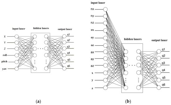
Figure 8. Neural network architecture: (a) RPY NN; (b) MATRIX NN.

2.3. The Amount of Training Data

The basic rule for selecting training data says that the number of observations should be ten times the number of connections in the NN. However, in practice, this amount of data also depends on the complexity of the task that the neural network must predict. With an increase in the number of variables, the number of required observations grows non-linearly, so even with a fairly small number of variables, a fairly large number of observations may be required [18,19].

Let us analyze the required amount of input data for training a neural network designed to solve the IKP. The research will be conducted on 1000, 10,000, 40,000, and 160,000 values of training datasets.

According to the standard approach, the input data is divided into the following proportion: 70% are used as training data, 15% as validation data, and 15% are used for testing [20]. The duplicate input data should be removed [20].

2.4. The Activation Function

The activation function determines the output value of the neuron depending on the result of the weighted sum of the inputs and some threshold value [21].

To solve the regression problem and neural network training using gradient descent, we need a differentiable activation function. It is recommended to choose a sigmoid function. However, since the neural network being designed should perceive values both in the positive and in the negative range, therefore, despite all the advantages of the sigmoid function we will lose some of the data.

For the designed neural network, we need an activation function that will repeat all the properties of the sigmoid function but lie in the range from −1 to 1. For this task, we will use the hyperbolic tangent function $th(x)=\frac{e^{2x}-1}{e^{2x}+1}$. Using this function will allow us to switch from the binary outputs of the neuron to analog ones. The range of values of the hyperbolic tangent function lies in the interval (−1; 1).

In MATLAB, we will use the tansig(x) function, which is equivalent to the function that implements the hyperbolic tangent tanh(x). At the same time, the function tansig(x) is calculated faster than tanh(x), however, the solutions may have minor deviations [22]. The use of the tansig(x) function is a good alternative for developing neural networks in which the speed of calculations is important, rather than the accuracy of calculating the activation function [23].

2.5. The Loss Function

To check the correctness of the solutions obtained from the neural network, we must calculate the deviations of the neural network solution from the solutions obtained as a result of solving IKP. To do this, we will use the loss function.

To calculate the error, we use the Mean Squared Error (MSE) method

$$MSE=\frac{1}{n}{\displaystyle \sum _{i=1}^n{(y_k-y_n)}^2},$$

(7)

where $y_k$ are the true output values of the robot, $y_n$ are the output values that the NN received, $n$ is the total amount of data.

Usually, outliers in the training dataset are discarded. Since our robot is limited by the physical capabilities of the servo drives (Table 2), there will be no anomalous values in the dataset.

The MSE method performs well at a fixed learning rate [24].

2.6. The Learning Functions

To select the optimal learning algorithm, traditionally the main indicators are its accuracy and performance. As a neural network training algorithm for solving IKP, the use of the following types of error backpropagation methods were studied:

• Levenberg–Marquardt (trainlm);
• Bayesian regularization backpropagation (trainbr);
• scaled conjugate backpropagation gradient (trainscg);
• resilient backpropagation (trainrp).

To select an algorithm, the solution was tested on training a simple network—a MATRIX NN with 40,000 values of training datasets.

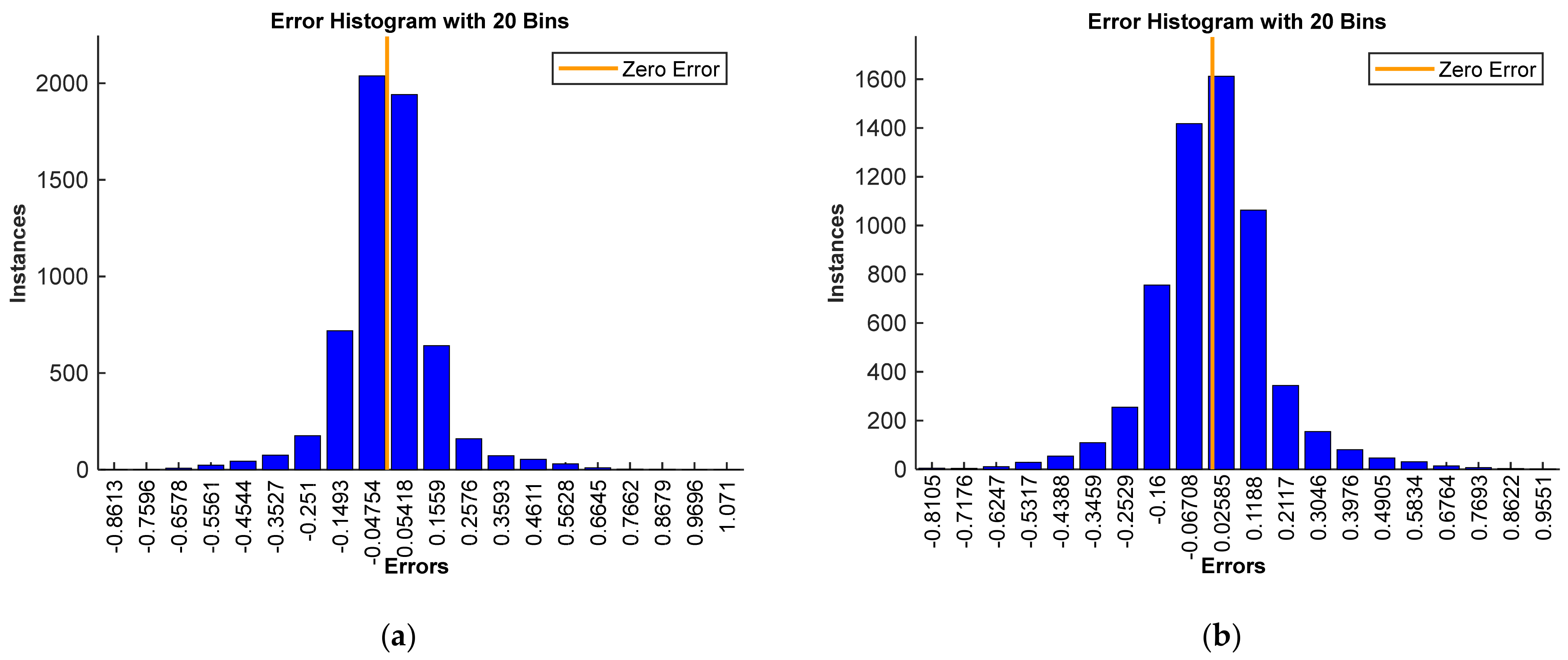
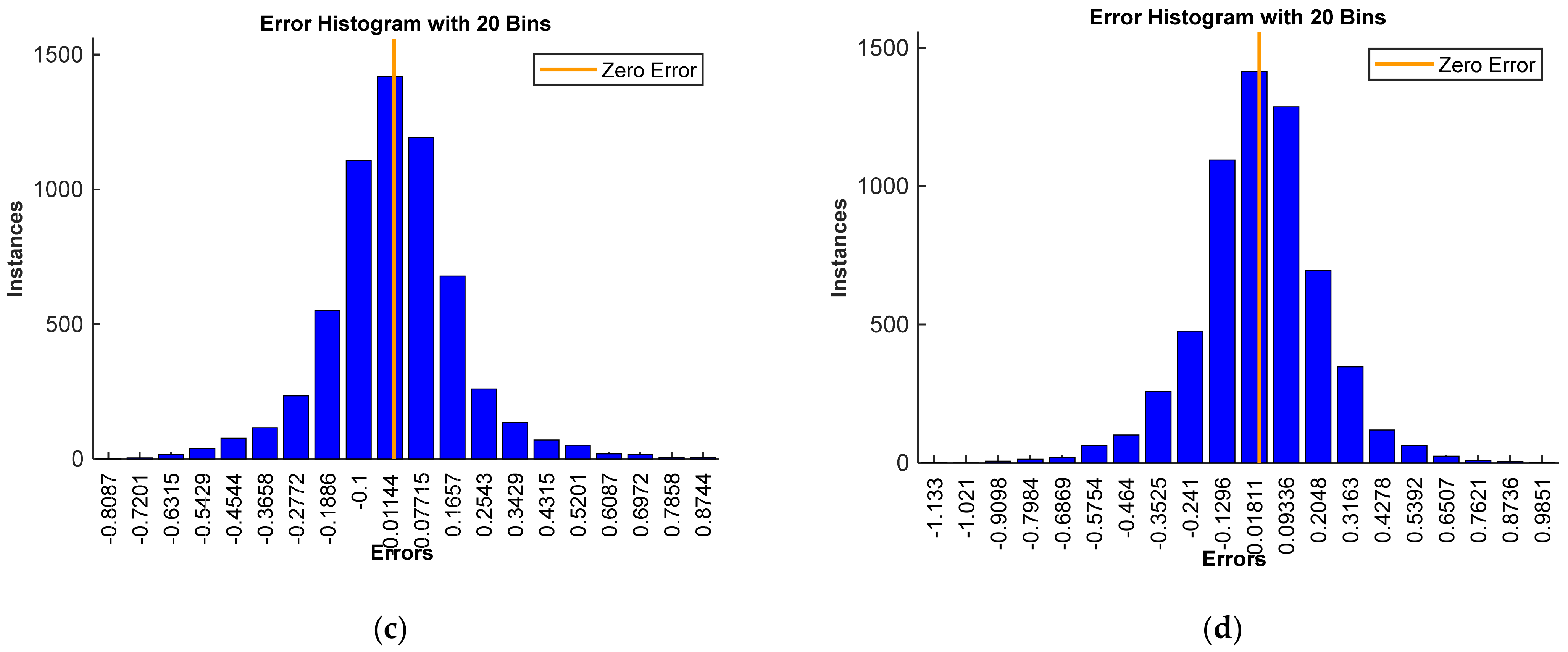
Figure 9 shows error histograms as the difference between target and predicted values when training a MATRIX NN with 40,000 values of training datasets using the indicated algorithms.

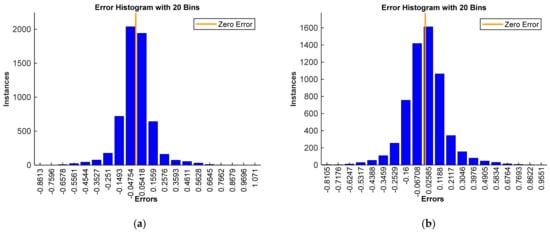
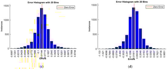
Figure 9. Error histogram as the difference between the target and predicted values when training a neural network using: (a) the Levenberg–Marquardt (trainlm); (b) the Bayesian regularization backpropagation (trainbr); (c) scaled conjugate backpropagation gradient (trainscg); (d) resilient backpropagation (trainrp).

The mathematical expectations of errors for each of the algorithms are shown in Table 3. It shows that the best result was shown by the Levenberg–Marquardt algorithm, which provides fast convergence of the learning error. In further studies, we will use this learning function.

Table 3. Mathematical expectations of NN training algorithms.

Algorithm	The Mathematical Expectation of Error (m)
trainlm	0.0786
trainbr	0.0852
trainscg	0.1242
trainrp	0.1045

Note that the Levenberg–Marquardt algorithm is the fastest backpropagation algorithm in the MATLAB Neural Network Toolbox and is recommended for use even though it requires more RAM than other algorithms.

2.7. The Hidden Layers

Usually, the search for the optimal dimension for the hidden layer is determined experimentally [20]. At the same time, too many neurons are undesirable, because this can lead to overfitting. However, the number of neurons should be sufficient so that the neural network can capture the complexity of the input–output connections.

In [25], three rules are mentioned for choosing the dimension of the hidden layer:

• if there is only one output node in the neural network, and it is assumed that the required input–output connection is quite simple, then at the initial stage the dimension of the hidden layer is assumed to be 2/3 of the dimension of the input layer;
• if the neural network has several output nodes or it is assumed that the required input–output relationship is complex, the dimension of the hidden layer is taken equal to the sum of the input dimension plus the output dimension (but it must remain less than twice the input dimension).
• if in the neural network the required input–output connection is extremely complex, then the dimension of the hidden layer is set equal to one less than twice the input dimension.
• Based on the above recommendations, we will set the configuration of the hidden layer:
• the number of hidden layers is one;
• the number of neurons in this layer is set to one less than twice the input dimension.

Based on the above recommendations, Table 4 shows the parameters of neural networks and the results of their training, which were studied to select the best option.

Table 4. Results of training neural networks.

Experiment N	Amount of Training Data	Number of Hidden Layers	Number of Neurons in Hidden Layers	Loss Function (m)
				RPY NN	MATRIX NN
1	40,000	1	(11-RPY) (23-MATRIX)	0.0836	0.0384
2	40,000	2	[20,30]	0.0259	0.0166
3	40,000	4	[30,30,60,60]	0.0119	0.0110
4	160,000	4	[30,30,60,60]	0.0094	0.0068

The studies have shown a higher accuracy of the MATRIX NN. For this network, in the case of 160,000 inputs, the error is 0.0068 m. For the RPY NN in a similar situation, the error is 0.0094 m. Additionally, note that the training time of the RPY NN without connecting a graphics processing unit (GPU) is approximately 10 times longer than the training time of the MATRIX NN. In the future, all reasoning will be carried out for the network, with input values taken for the MATRIX NN.

For the proposed structure of the MATRIX NN, good results were obtained, but the deviation in the size of 0.0068 m will not allow the use of the manipulator when performing the technological operation that requires higher accuracy.

3. Results

3.1. The “Correctional” Neural Network

Since the use of large NN with large input datasets requires the use of large computing resources, we will improve the accuracy of solution not by increasing the NN, but by changing the configuration of the NN.

In most applications, the manipulator always starts motion from some arbitrary position and moves along a trajectory from successive points. Including the current manipulator configuration in the input data has a positive effect on estimating the joint angles for the next desired position. We will artificially divide the trajectory of the manipulator to a given point into two parts. The first part is the arrival of the manipulator in the area as close as possible to the desired point and the second part is the adjustment of the manipulator to the desired point (Figure 10).

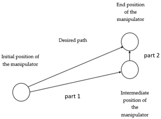
Figure 10. The manipulator movement to a given point.

Based on this idea, in this paper we propose a new design of the NN to solve the IKP for an anthropomorphic manipulator. To improve the accuracy of the IKP solution we propose to take into account the values of the manipulator generalized coordinates that are close to the desired ones, assuming them as the current values of the manipulator joints angles. The new design of the NN is based on the use of the so-called “correctional” structure of the NN. It consists of the MATRIX NN described above and the second series-connected NN. The input of the second series-connected network will supply the same values as for the MATRIX NN and the output of the MATRIX NN (Figure 11), which gives us close to the desired values of the generalized coordinates of the manipulator.

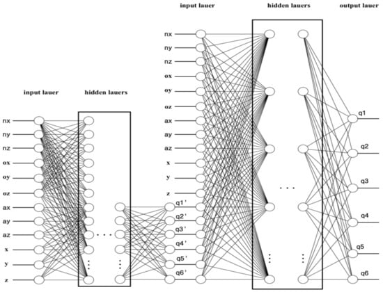
Figure 11. The correctional NN.

The proposed NN (Figure 11) has 12 elements in the input layer (data from the MATRIX NN). The output layer has six elements, generalized coordinates, which represent the joint’s angles. Eighteen input data values are fed to the input of the second network:

$$X_2=[n_x n_y n_z o_x o_y o_z a_x a_y a_z x y z {q^{\prime }}_1 {q^{\prime }}_2 {q^{\prime }}_3 {q^{\prime }}_4 {q^{\prime }}_5 {q^{\prime }}_6].$$

The inputs and outputs of the correctional NN (Figure 11) are described as follows:

$$\begin{array}{c}[Q^{\prime }]=ANN\_Net1(R_{3x3} p_{3x1}).\\ [Q^{\prime }]=ANN\_Net1(n_x n_y n_z o_x o_y o_z a_x a_y a_z x y z ),\\ [Q]=ANN\_Net2(R_{3x3} p_{3x1}, Q^{\prime }), Q^{\prime }=[{q^{\prime }}_1 {q^{\prime }}_2 {q^{\prime }}_3 {q^{\prime }}_4 {q^{\prime }}_5 {q^{\prime }}_6], Q=[q_1 q_2 q_3 q_4 q_5 q_6].\end{array}$$

(8)

To test the solution of the correctional NN, we use new randomly obtained positions of the robot SAR-401 manipulator, which were not used for training. This is necessary to check for overfitting.

We will check the accuracy using the DKP. Having tested the operation of the NN with a new random input data set, we found that the root-mean-square error is 0.0035 m (Figure 12a).

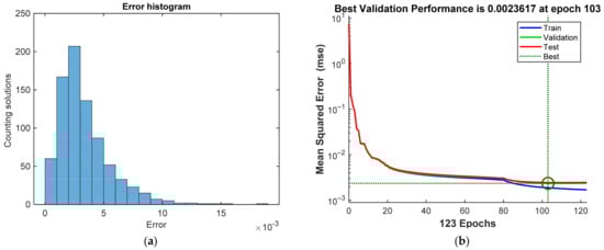
Figure 12. (a) The correctional NN error propagation histogram (b) The performance of the correctional NN.

The performance of the correctional NN is shown in Figure 12b. The differences between the NN output and the target are computed via the MSE. It decreases rapidly during the learning process.

3.2. Example

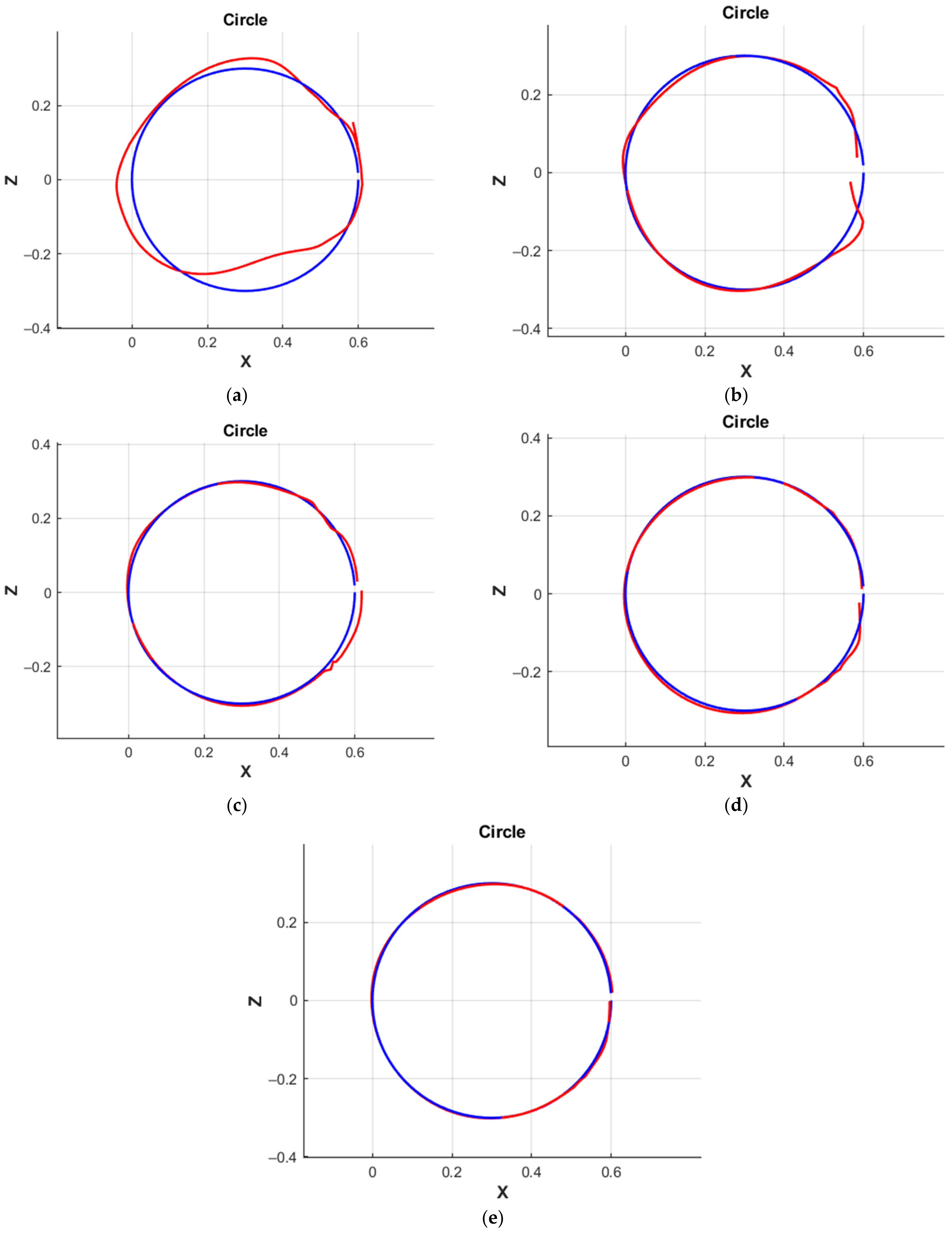
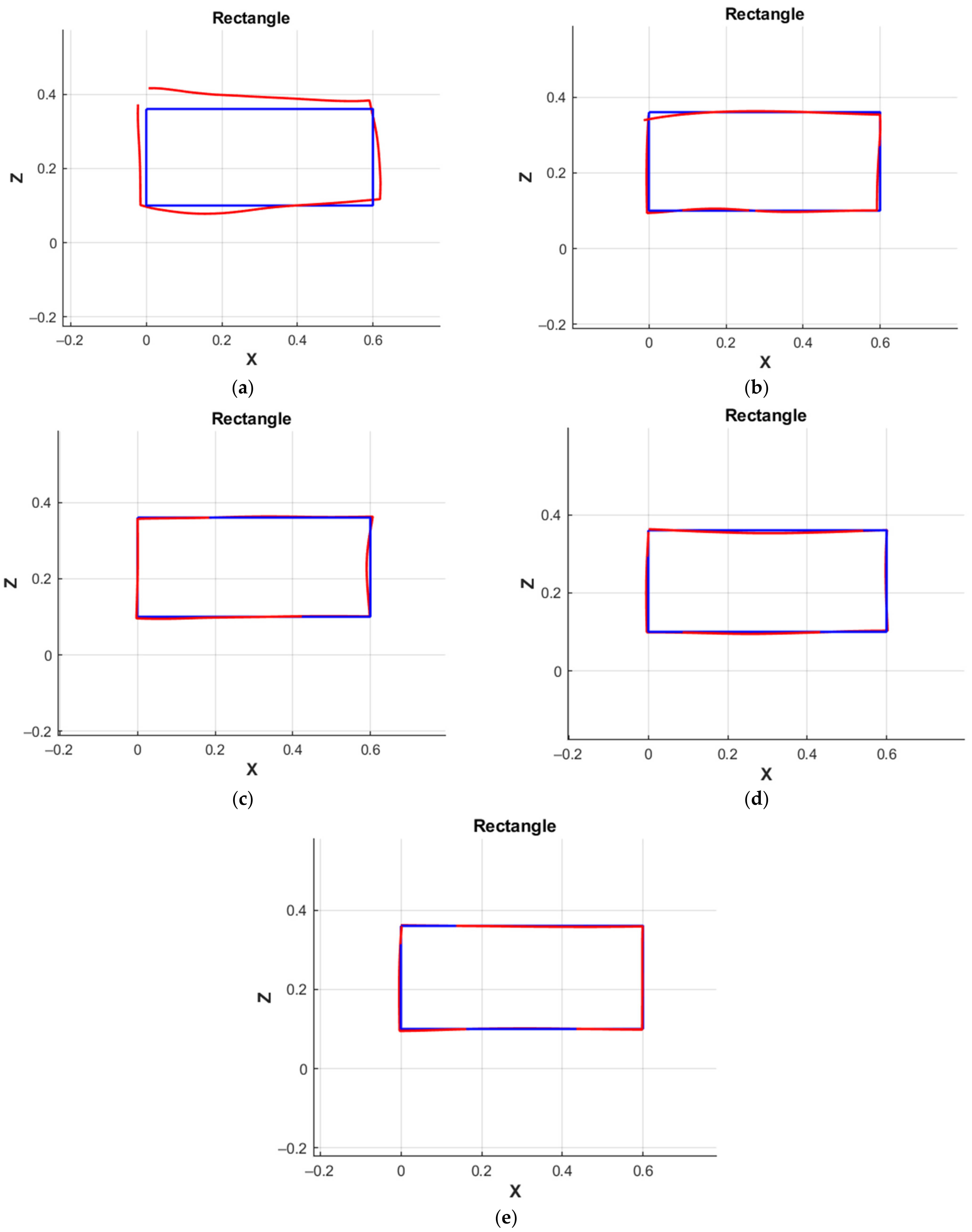
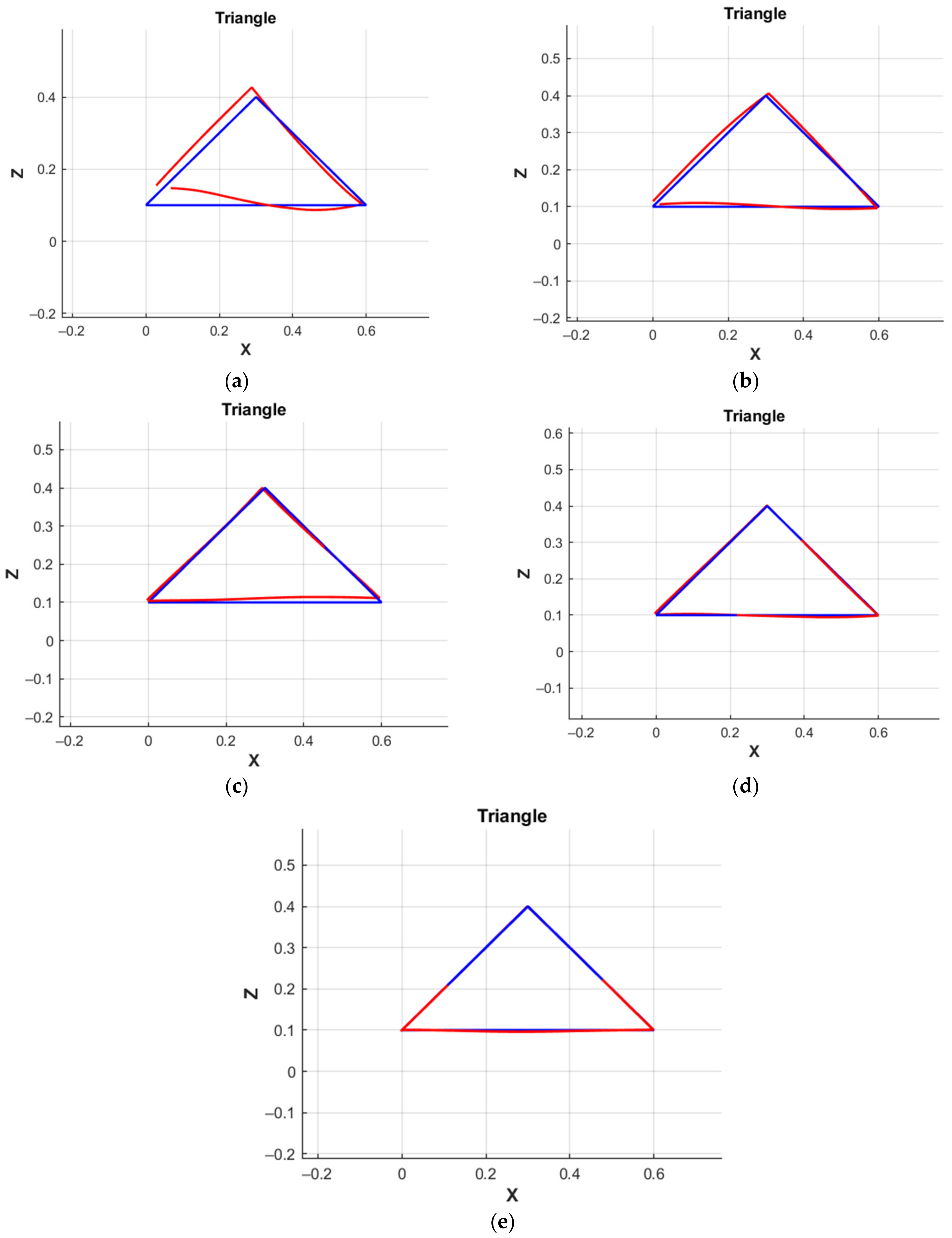
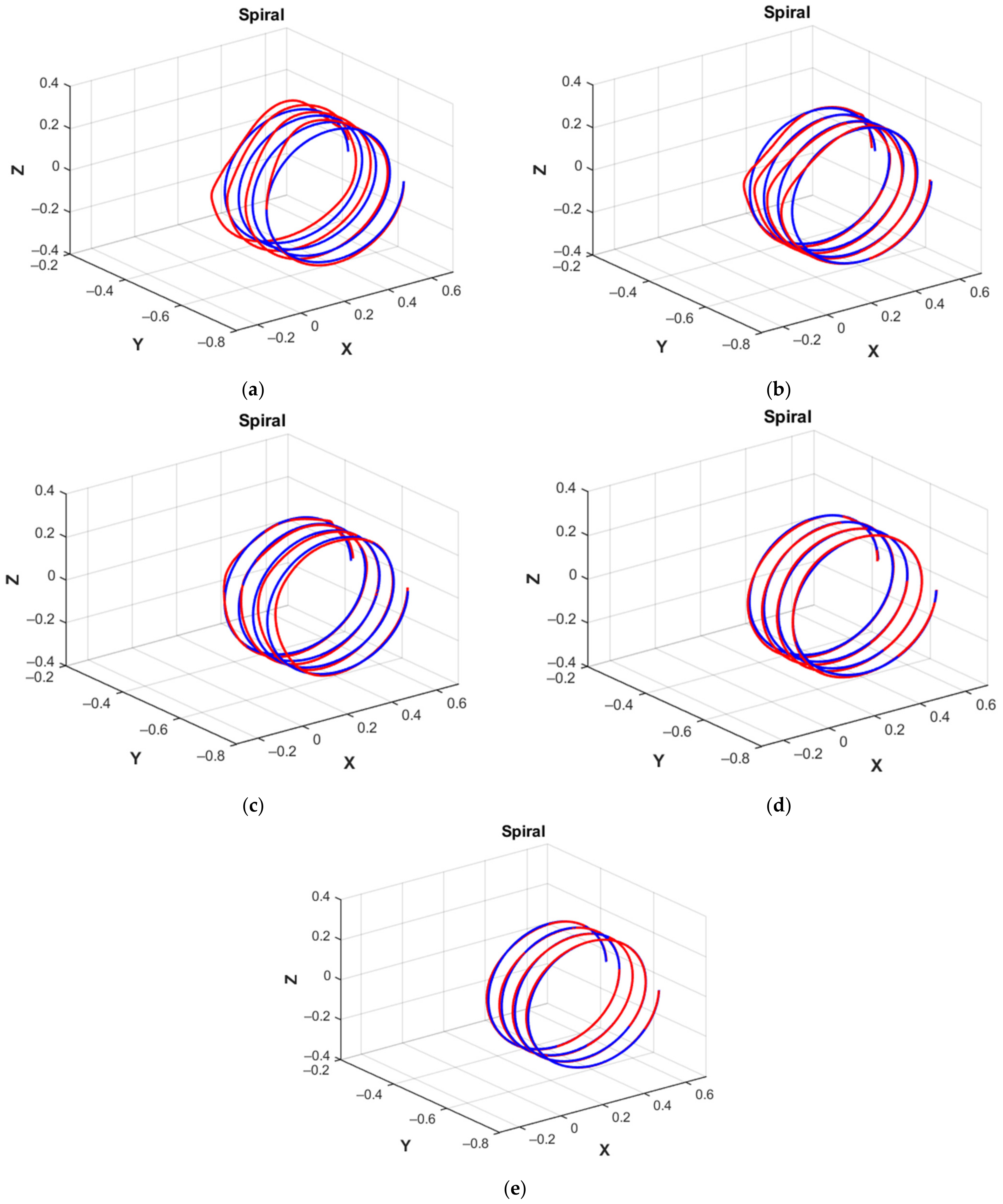
After training the correctional NN, we will conduct experiments by calculating various movements of the robot SAR-401 manipulator, using this NN for solving the IKP. Let us move the manipulator along the trajectories: a circle, a triangle, a rectangle, and a 3D spiral, moving forward along the Y-axis. The experiments were performed in MATLAB, on the robot SAR-401 simulator, and the robot SAR-401.

We will demonstrate the solution of these problems for various variants of MATRIX NN (see Table 4) and the correctional NN.

In Figure 13, Figure 14, Figure 15 and Figure 16 we present a graphical solution of these problems for each of the NNs in comparison with the solution of the IKP. In all graphs, the solution of the neural network is marked in red, and the construction of the trajectory using the IKP is marked in blue.

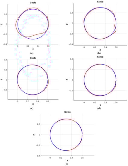
Figure 13. Simulation of the movement of the manipulator along a circle: (a) MATRIX NN 1; (b) MATRIX NN 2; (c) MATRIX NN 3; (d) MATRIX NN 4; (e) the correctional NN.

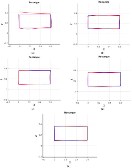
Figure 14. Simulation of the movement of the manipulator along the rectangle: (a) MATRIX NN 1; (b) MATRIX NN 2; (c) MATRIX NN 3; (d) MATRIX NN 4; (e) the correctional NN.

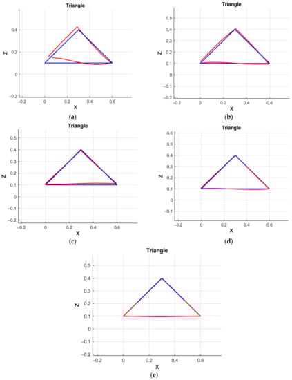
Figure 15. Simulation of the movement of the manipulator along the triangle: (a) MATRIX NN 1; (b) MATRIX NN 2; (c) MATRIX NN 3; (d) MATRIX NN 4; (e) the correctional NN.

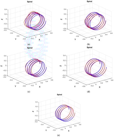
Figure 16. Simulation the movement of the manipulator in a 3D spiral: (a) MATRIX NN 1; (b) MATRIX NN 2; (c) MATRIX NN 3; (d) MATRIX NN 4; (e) the correctional NN.

It is also possible to demonstrate the movement of the manipulator in MATLAB. An example of a demonstration is shown in Figure 17.

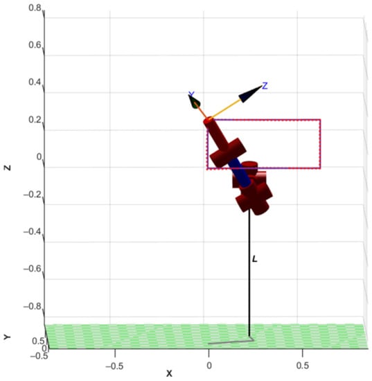
Figure 17. The demonstration of the movement of the manipulator in MATLAB.

Figure 18 shows the simulator, in which manipulator control was tested using the correctional NN.

Figure 18. Testing the NN on the SAR-401 simulator.

Note that the time for calculating the classical solution of the IKP when calculating 400 points for the 3D spiral trajectory was from 33 to 42 s. The time for calculating the same points of the trajectory using the NN lies in the interval from 0.06 to 0.3 s.

The classical numerical solution of the IKP and the solution of the IKP using the NN have some discrepancies (error) (this is seen from Figure 13, Figure 14, Figure 15 and Figure 16).

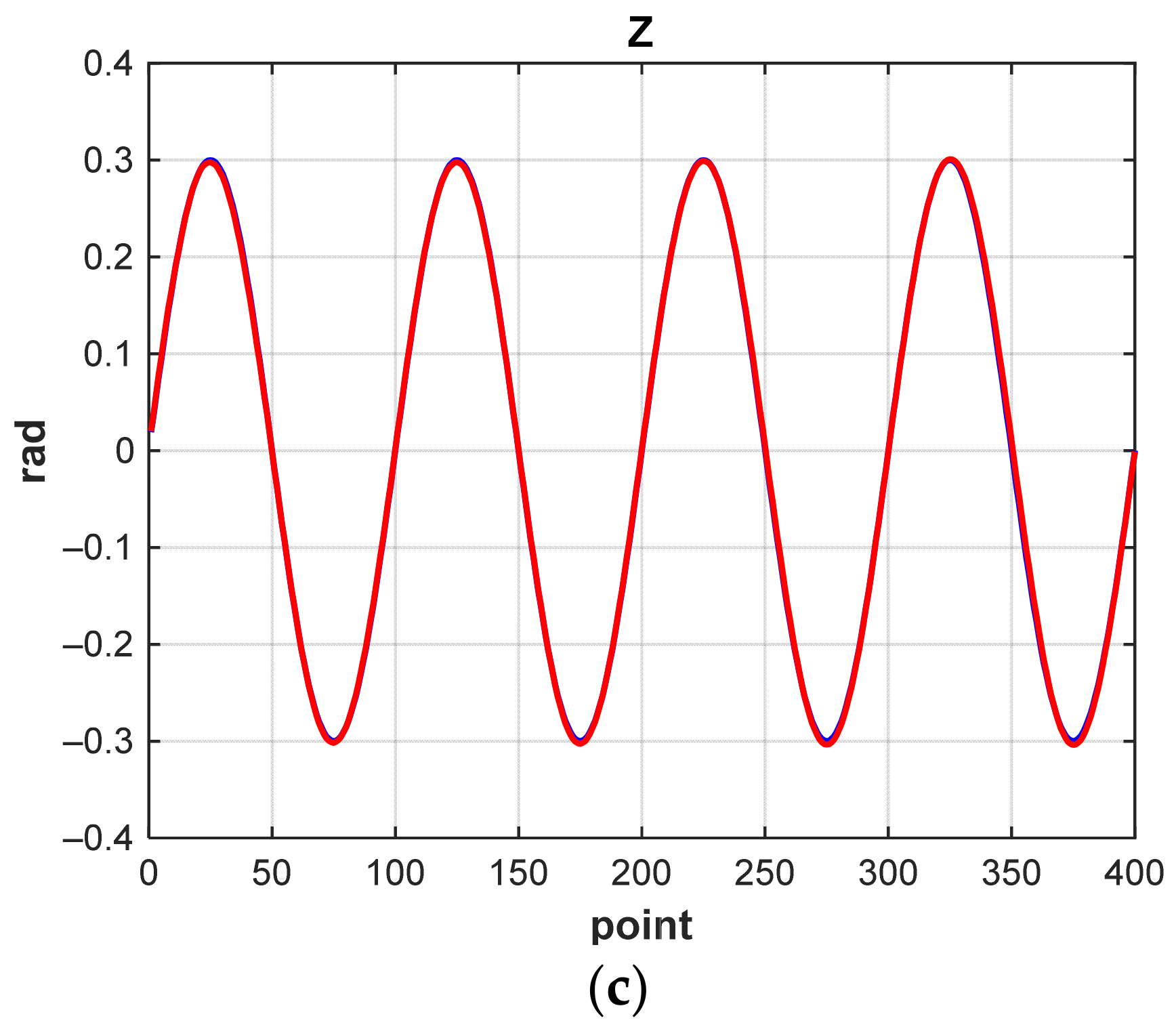
Let us demonstrate in Figure 19 and Figure 20 graphs of changes in X, Y, and Z coordinates when the manipulator moves along a 3D spiral for MATRIX NN 1 and the correctional NN. In all graphs, the solution of the NN is marked in red, and the construction of the trajectory using the IKP is marked in blue.

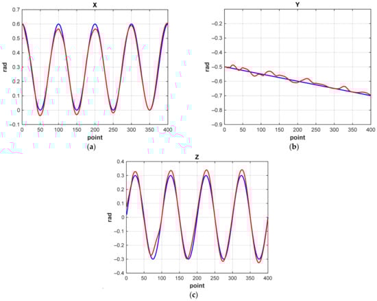
Figure 19. Graphs of changes in coordinates when the manipulator moves in a 3D spiral (MATRIX NN 1): (a) along the X-axis; (b) along the Y-axis; (c) along the Z-axis.

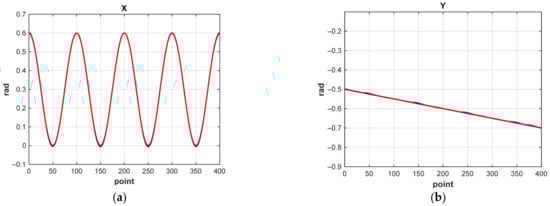
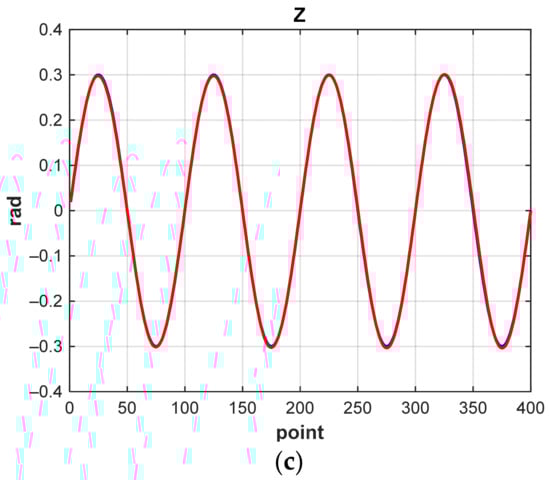
Figure 20. Graphs of coordinate changes during the movement of the manipulator in a spiral in 3D (the correctional NN): (a) along the X-axis; (b) along the Y-axis; (c) along the Z-axis.

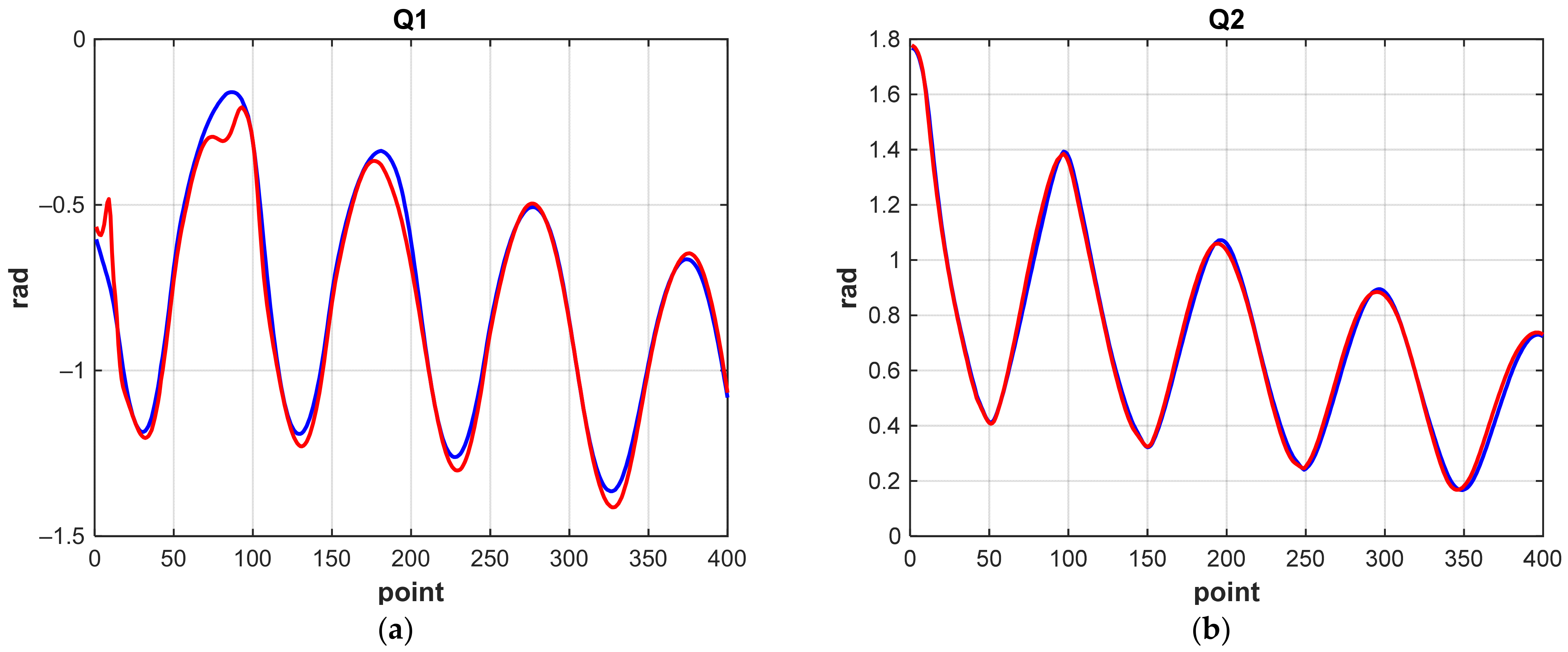
Certain conclusions can be drawn by analyzing changes in the generalized coordinates of the manipulator, which explain which joint makes the greatest contribution to the error. Figure 21 and Figure 22 show the corresponding graphs. As before, the solution of the neural network is marked in red, and the construction of the trajectory using the numerical solution of the IKP is marked in blue.

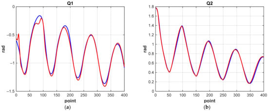
Figure 21. Graphs of changes in generalized coordinates when the manipulator moves along a 3D spiral (MATRIX NN 1): (a) q1; (b) q2; (c) q3; (d) q4; (e) q5; (f) q6.

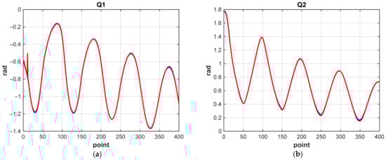
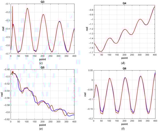
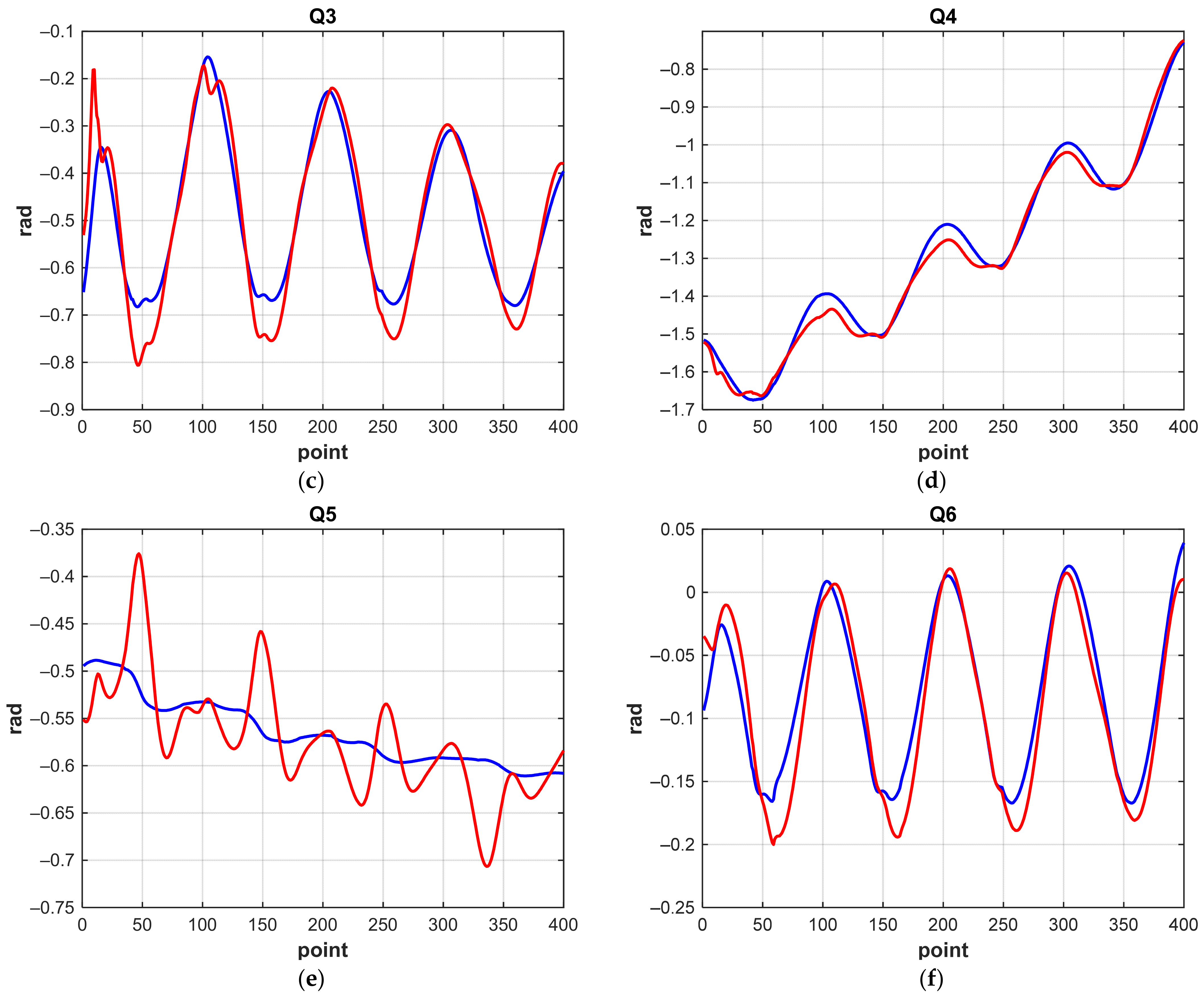
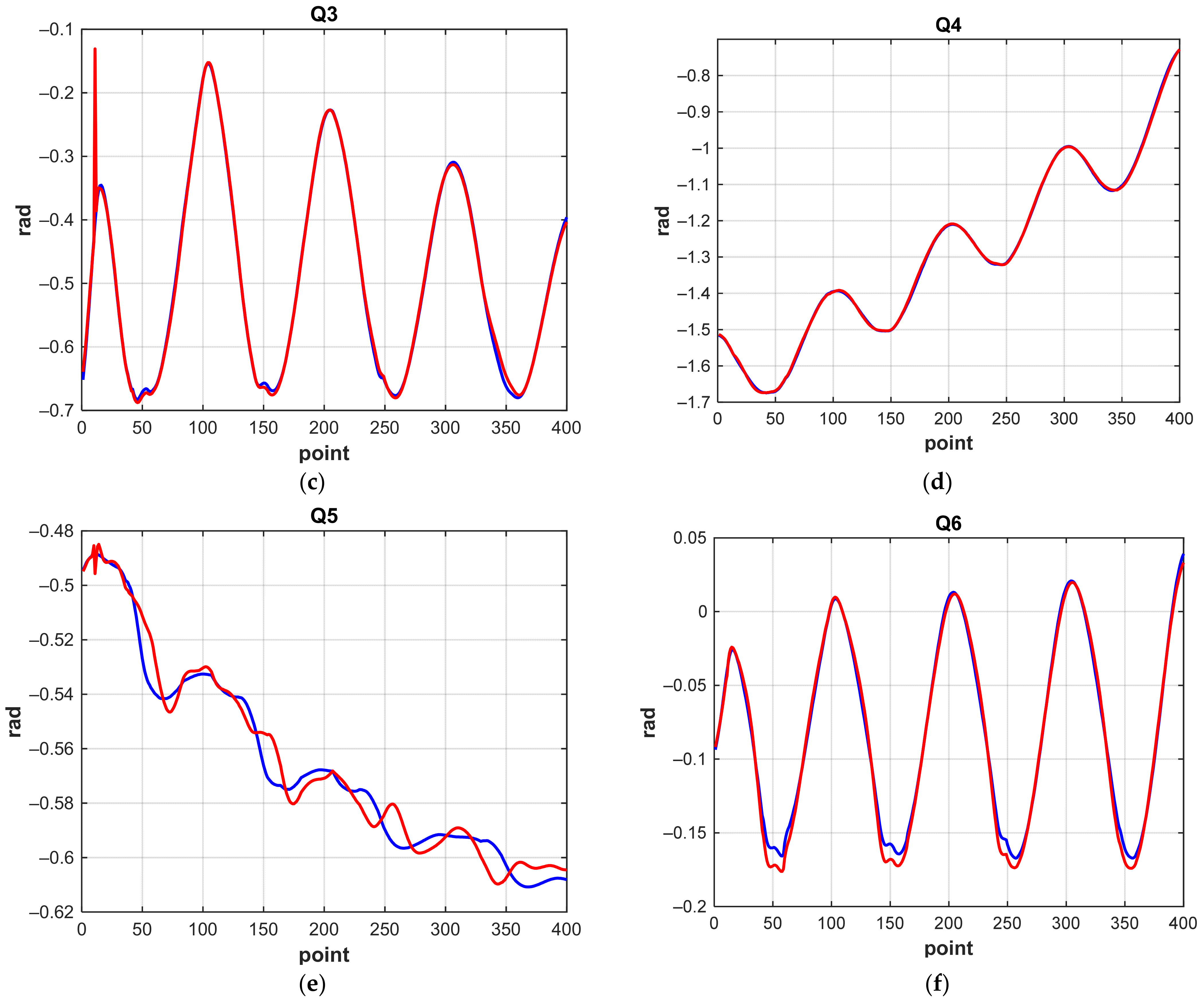
Figure 22. Graphs of changes in generalized coordinates when the manipulator moves along a 3D spiral (the correctional NN): (a) q1; (b) q2; (c) q3; (d) q4; (e) q5; (f) q6.

We see that a significant contribution to the error is made by the q5 coordinate (Figure 5), which determines the rotation of the “wrist” of the manipulator. Calculation accuracy and NN characteristics are shown in Table 5. The accuracy of 2–4 mm obtained by correctional NN is sufficient for the manipulation tasks of the SAR-401 robot and is related to mechanical characteristics (backlash, friction, etc.). The specified error allows the robot to capture objects and perform manipulation operations.

Table 5. The IKP NN prediction accuracy.

Neural Network	Amount of Training Data	Number of Hidden Layers	Number of Neurons in Hidden Layers	Calculation Accuracy (m)
				Spiral	Triangle	Rectangle	Circle
MATRIX NN 1	40,000	1	23	0.0347	0.0358	0.0342	0.0483
MATRIX NN 2	40,000	2	[20,30]	0.0168	0.0162	0.0094	0.0156
MATRIX NN 3	40,000	4	[30,30,60,60]	0.0138	0.0077	0.0053	0.0112
MATRIX NN 4	160,000	4	[30,30,60,60]	0.0068	0.0043	0.0042	0.0070
The correctional NN	160,000	4 4	[30,30,60,60] [30,30,60,60]	0.0035	0.0021	0.0032	0.0035

4. Discussion

A feature of the neural network approach is that neural networks can be divided into different types according to different criteria. For example, from the point of view of the network structure, they can be divided into two categories: feedforward neural networks and recurrent neural networks [26]. To design neural networks, formalized algorithms are not always used. For example, they are not always used when choosing the number of hidden layers. This leads to the fact that the neural network is a design based on various tests and experiments. It is not always possible to find a universal approach. Despite this, if it is possible to find an effective neural network structure for solving the IKP for the type of anthropomorphic manipulator, then we will get a very effective solution in terms of algorithm speed and accuracy.

At the same time, the obtained solution can be complex in the sense that by solving the IKP using the NN approach, it is also possible to solve the problem of the self-collision control of manipulators using this approach. A feature of solving this problem will be its solution not with the help of a classification approach, but with the help of a regression method [19].

Therefore, for example, in the problem of the self-collision control, to collect training data, it is necessary to change the position of two manipulators in random order and obtain from the robot for each position of the manipulators the values of the coordinates and Euler angles of orientation in space of all nodes of the manipulators. Thus, as input data, we will use the values of the rotation angles of the servo drives for each joint of the two manipulators. The NN input dataset for the self-collision control problem will be the elements of the homogeneous transformation matrix (nine elements of the rotation matrix and three values of the position vector for each manipulator).

To calculate the output of the NN, all distances between the links of two manipulators are determined. The minimum distance between the manipulators for each position in the robot workspace for the corresponding input data is used as the output value.

When choosing a NN configuration and processing input data, we will get an effective integrated solution of the problem of anthropomorphic manipulators motion with the self-collision control based on a unified NN approach.

5. Conclusions

In this paper, we have solved the IKP for the robot SAR-401 anthropomorphic manipulator. To solve the problem, the NN was designed, and the input data of the NN are the elements of the homogeneous transformation matrix. The choice of the NN configuration was carried out using a comparative analysis. The solution obtained in this paper is characterized by high speed and accuracy. Given the presence of two manipulators in the robot SAR-401, when performing technological operations, self-collisions of manipulators may occur. The problem of self-collision control can also be solved based on the NN approach.

References

- Li, S.; Zhang, Y.; Jin, L. Kinematic control of redundant manipulators using neural networks. IEEE Trans. Neural Netw. Learn. Syst. 2017, 28, 2243–2254. [Google Scholar] [CrossRef] [PubMed]
- Hollerbach, J.; Suh, K. Redundancy resolution of manipulators through torque optimization. IEEE J. Robot. Automat. 1987, 3, 308–316. [Google Scholar] [CrossRef] [Green Version]
- Ahmed, R.J.; Almusawi, L.; Dülger, C.; Kapucu, S. A new artificial neural network approach in solving inverse kinematics of robotic arm (Denso VP6242). Comput. Intell. Neurosci. 2016, 2016, 5720163. [Google Scholar] [CrossRef] [Green Version]
- Bingul, Z.; Ertunc, H.M.; Oysu, C. Comparison Of Inverse Kinematics Solutions Using Neural Network for 6R robot Manipulator With Offset. In Proceedings of the ICSC Congress on Computational Intelligence Methods and Applications, Istanbul, Turkey, 15–17 December 2005; p. 5. [Google Scholar] [CrossRef]
- Xia, Y.; Wang, J. A dual neural network for kinematic control of redundant robot manipulators. IEEE Trans. Syst. Man Cybern. 2001, 31, 147–154. [Google Scholar] [CrossRef] [Green Version]
- Yang, Y.; Peng, G.; Wang, Y.; Zhang, H. A New Solution for Inverse Kinematics of 7-DOF Manipulator Based on Neural Network. In Proceedings of the IEEE International Conference on Automation and Logistics, Jinan, China, 18–21 August 2007. [Google Scholar] [CrossRef]
- Liu, J.; Wang, Y.; Li, B.; Ma, S. Neural network based kinematic control of the hyper-redundant snake-like manipulator. In Proceedings of the 4th International Symposium on Neural Networks, Nanjing, China, 3–7 June 2007. [Google Scholar] [CrossRef] [Green Version]
- Daya, B.; Khawandi, S.; Akoum, M. Applying neural network architecture for inverse kinematics problem in robotics. J. Softw. Eng. Appl. 2010, 3, 230–239. [Google Scholar] [CrossRef] [Green Version]
- Driscoll, J.A. Comparison of Neural Network Architectures for The Modelling Of Robot Inverse Kinematics. In Proceedings of the 2000 IEEE SOUTHEASTCON, Nashville, TN, USA, 7–9 April 2000; pp. 44–51. [Google Scholar] [CrossRef]
- Choi, B.B.; Lawrence, C. Inverse Kinematics Problem in Robotics Using Neural Networks; NASA Technical Memorandum; Lewis Research Center: Cleveland, OH, USA, 1992; Volume 105869. [Google Scholar]
- Peters, J.; Lee, D.; Kober, J.; Nguyen-Tuong, D.; Bagnell, J.A.; Schaal, S. Chapter 15. Robot learning. In Handbook of Robotic; Springer International Publishing: Cham, Switzerland, 2016. [Google Scholar]
- Alchakov, V.; Kramar, V.; Larionenko, A. Basic approaches to programming by demonstration for an anthropomorphic robot. IOP Conf. Ser. Mater. Sci. Eng. 2020, 709, 022092. [Google Scholar] [CrossRef]
- Bogdanov, A.; Dudorov, E.; Permyakov, A.; Pronin, A.; Kutlubaev, I. Control System of a Manipulator of the Anthropomorphic Robot FEDOR. In Proceedings of the 2019 12th International Conference on Developments in eSystems Engineering (DeSE), Kazan, Russia, 7–10 October 2019; pp. 449–453. [Google Scholar] [CrossRef]
- Kramar, V.A.; Alchakov, V.V. The methodology of training an underwater robot control system for operator actions. J. Phys. Conf. Ser. 2020, 1661, 012116. [Google Scholar] [CrossRef]
- Kramar, V.; Kabanov, A.; Kramar, O.; Putin, A. Modeling and testing of control system for an underwater dual-arm robot. IOP Conf. Ser. Mater. Sci. Eng. 2020, 971, 042076. [Google Scholar] [CrossRef]
- Denavit, J.; Hartenberg, R.S. A kinematic notation for lower-pair mechanisms based on matrices. Trans. ASME J. Appl. Mech. 1955, 23, 215–221. [Google Scholar] [CrossRef]
- Corke, P.I. Robotics, Vision and Control Fundamental Algorithms in Matlab; Springer: Cham, Switzerland, 2017; p. 693. [Google Scholar] [CrossRef]
- Chen, D.; Cheng, X. Pattern Recognition and String Matching; Springer-Verlag: New York, NY, USA, 2002; p. 772. [Google Scholar] [CrossRef]
- Haykin, S. Neural Networks a Comprehensive Foundation, 2nd ed.; Prentice-Hall: Hoboken, NJ, USA, 1999; p. 842. [Google Scholar]
- Ng, A. Machine Learning Yearning; GitHub eBook (MIT Licensed): San Francisco, CA, USA, 2018; p. 118. [Google Scholar]
- Szandała, T. Review and comparison of commonly used activation functions for deep neural networks. In Bio-Inspired Neurocomputing. Studies in Computational Intelligence; Bhoi, A., Mallick, P., Liu, C.M., Balas, V., Eds.; Springer: Singapore, 2021; pp. 203–224. [Google Scholar] [CrossRef]
- Rumelhart, D.; Hintont, G.; Williams, R. Learning representations by back-propagating errors. Nature 1986, 323, 533–536. [Google Scholar] [CrossRef]
- Nwankpa, C.E.; Ijomah, W.; Gachagan, A.; Marshall, S. Activation functions: Comparison of trends in practice and research for deep learning. In Proceedings of the 2nd International Conference on Computational Sciences and Technology, Jamshoro, Pakistan, 17–19 December 2020. [Google Scholar]
- Irwin, G.W.; Warwick, K.; Hunt, K.J. Neural network applications in control. IEE Control Eng. Ser. 1995, 53, 309. [Google Scholar]
- Heaton, J. Artificial Intelligence for Humans; Heaton Research, Incorporated: St. Louis, MO, USA, 2015; p. 374. [Google Scholar]
- Müller, B.; Reinhardt, J.; Strickland, M.T. Neural Networks: An Introduction; Springer: New York, NY, USA, 2012. [Google Scholar]
Publisher’s Note: MDPI stays neutral with regard to jurisdictional claims in published maps and institutional affiliations. |
© 2022 by the authors. Licensee MDPI, Basel, Switzerland. This article is an open access article distributed under the terms and conditions of the Creative Commons Attribution (CC BY) license (https://creativecommons.org/licenses/by/4.0/).