Design and Control of a Hydraulic Hexapod Robot with a Two-Stage Supply Pressure Hydraulic System

Abstract

This paper focuses on the system design and control strategies of a hydraulic hexapod robot (HHR) ZJUHEX01 with a two-stage supply pressure hydraulic system (TSS). Firstly, a brief introduction is given, including the mechanical structure, the onboard hydraulic system, and the control system architecture. Secondly, the kinematics model and hydraulic system model are built in preparation for the controller design. Then a sliding mode repetitive controller (SMRC) for the separate meter in and separate meter out (SMISMO) hydraulic system is proposed, as well as the valve configuration, to help HHR get better control performance and smaller tracking errors. Furthermore, a high order sliding mode differentiator (HOSMD) is developed to obtain the joint angular velocity and acceleration. Finally, the ADAMS and MATLAB/Simulink co-simulation model is established to verify the effectiveness of the control strategy. Also, the energy consumption of TSS is compared with that of one-stage supply pressure hydraulic system (OSS) to show a great energy-saving effect of 51.94%.

1. Introduction

Multilegged robots possess superior mobility in challenging environments and uneven terrain where wheeled and tracked vehicles cannot reach [1]. Compared with quadruped robots, hexapod robots are able to own high stability and capacity at the expense of certain dynamic performance owing to their tripod gaits [2]. With the help of hydraulic actuation, hydraulic hexapod robots (HHR) can provide large force output, as well as high power density and strong robustness, which is suitable for heavy load occasions and disaster-rescue tasks. However, higher complexity and cost, as well as the low energy efficiency, are the critical issues restricting the widespread use of hydraulic legged robots [3].

Since Boston Dynamics created a hydraulic quadruped BigDog in 2005 [4], various research centers, universities, and industries have proposed their hydraulic quadruped robot, such as HyQ series [5,6,7], JINPOONG [8], SCalf series [9,10,11], Baby-elephant [12], MBBOT [13], NUDT quadruped robot [14], BIT quadruped robot [15], etc. In terms of HHR, COMET series [16,17], HexaTerra [18], LSHDSL-robot [19], etc. Dynamic motion is the fundament for hydraulic walking robots performing different tasks; therefore, various control strategies have been proposed. Cunha et al. [20] combined the gain scheduling algorithm with PID controller in the HyQ leg prototype. Focchi et al. [21] compared the control performance of the conventional PID, the linear quadratic regulator (LQR) controller, and the feedback linearization (FL) controller in the HyQ leg prototype. Bin et al. [22] applied self-tuning fuzzy-PID in the hydraulic quadruped robot leg prototype. Ke et al. [23] designed a feed-forward paralleled Active Disturbance Rejection Controller (ADRC) for foot-end-force control of the support leg of NUDT quadruped robot. Barai et al. [24] proposed a robust adaptive fuzzy controller with self-tuned adaptation gain in the hydraulic hexapod robot COMET-III. Irawan et al. [17] designed a position-based impedance controller for the leg and a center of mass-based impedance controller for the hydraulic hexapod robot COMET-IV. Wei et al. [25] designed a robust adaptive dynamic surface controller in the hydraulic quadruped robot hip joint. Wang et al. [26] adopted a fuzzy sliding mode controller in the hydraulic quadruped robot. Quan et al. [27] used a decoupling control strategy based on the diagonal matrix method in the hydraulic drive unit of a quadruped robot. Gao et al. [28] designed a neural network (NN) model reference decoupling controller to reduce the influence of the coupling of the hydraulically driven quadruped robot. Liu et al. [29] proposed a PID compound controller with velocity feedforward compensation (VFC) in the hydraulic wheeled-legged robot WLBOT. Apart from that, much research has also been done on force control and compliance control.

Though hydraulic legged robots have unparalleled advantages in high power density and robustness, their energy efficiency is still worse than animals with similar masses [30]. Nowadays, methods of reducing the energy consumption of hydraulic legged robots are as follows: (1) Optimization of mechanical and hydraulic system structure; (2) Optimization of motion planning; (3) Energy-saving and energy-recovery control strategies of the hydraulic system. Zhai et al. [31] proposed an archive-based micro genetic algorithm (AMGA) to optimize the mechanical structure and gait parameters, which shows a 40% energy-consumption decrease compared with the original structure. Barasuol et al. [32] designed a hydraulic integrated smart actuator (ISA) V5 to realize a power saving of approximately 112 W per actuator. Hua et al. [33] designed a hydraulic servo actuator with passive compliance (HPCA) in the hydraulic quadruped robot, which can help save more than 80 J energy in two gait cycles. Dong et al. [34] proposed a centroid fluctuation gait that can save more than 10% energy. Yang et al. [35] studied a foot trajectory based on the Fourier series to reduce about 7.55% joint energy consumption. Deng et al. [36] proposed a low energy cost foot trajectory planning method to realize a constant velocity of the body of a hydraulic hexapod robot which could reduce about 39% peak power. Tani et al. [37] proposed a method of taking the characteristics of the limited powered pump into consideration when designing the walking trajectory of a hydraulic legged robot, which could improve the energy efficiency and achieve power matching. Guglielmino et al. [38] established a hydraulic equivalent of the DC-DC switching Buck converter for the HyQ leg prototype to save about 75% energy. Xue et al. [39] designed a double-stage energy supply system using small accumulators to meet the instant high-pressure demands of hydraulic legged robots.

On the above issues of hydraulic legged robots, this paper concentrates on the design and control strategies of a hydraulic hexapod robot (HHR) with a two-stage supply pressure hydraulic system (TSS), especially on joint sliding mode repetitive control (SMRC) and energy-saving efficiency. In summary, the main contributions made are as follows:

• A SMRC controller is designed to improve the joint trajectory tracking performance;
• The high order sliding mode differentiator (HOSMD) is designed to help get the angular velocity and acceleration of HHR;
• A two-stage supply pressure hydraulic system (TSS) is utilized in HHR to save the energy of legs in the swing phase.

The remainder of this paper is structured as follows:

Section 2 gives an overview of the HHR system, including its mechanical structure, hydraulic system, and control system. Section 3 establishes the kinematics model and hydraulic model of HHR. Section 4 introduces the configuration of different valves in TSS and SMRC joint controllers. Section 5 describes the effectiveness of the control algorithm and energy-saving in ADAMS and MATLAB/Simulink co-simulation. A conclusion is offered in Section 6.

2. HHR System Overview

2.1. Mechanical Structure

HHR ZJUHEX01 can walk in different gaits to overcome irregular terrains and gain better environmental adaptability. Compared with the quadruped robot, HHR has higher stability and a larger load capacity for three grounded legs can always be obtained in tripod gaits ideally. As Figure 1 shows from the right side of HHR, it has a size of about 1.65 m (L) × 1.1 m (W) × 1.5 m (H) at the standard standing position and a total of about 1100 kg weight with an extra load capability of about 200 kg. The robot consists of a trunk and six legs, while all of them adopt the same mechanism, which consists of three DOFs (degree of freedom), including root abduction/adduction (RAA), hip flexion/extension (HFE), and knee flexion/extension (KFE). Additionally, each leg contains a spring damping foot, which can attenuate the shock and vibration and thus improve the energy utilization during locomotion.

2.2. Onboard Hydraulic System

HHR usually walks in tripod gait, which means three legs work in the stance phase while others are in the swing phase. Legs in the stance phase need to provide enough output force to support the whole HHR and meet locomotion requirements, while other legs in the swing phase are only supposed to overcome their gravity and dynamic force. Traditionally, a hydraulic walking robot consists of a one-stage supply pressure hydraulic system (OSS) which will cause extremely huge energy waste. As a result, a two-stage supply pressure hydraulic system (TSS) is proposed in Figure 2 to improve energy efficiency.

As is shown in Figure 2, TSS consists of a high-pressure pump (18 MPa) and a low-pressure pump (6 MPa), which will help HHR adapt to different load requirements in either the stance phase or swing phase. Each robot leg comprises three joint units including the knee, hip, and root. Both the knee and the hip adopt the same structure, where three directional control valves combine with an actuator to form a separate meter in and separate meter out (SMISMO) control system. As for the little movement and energy consumption of the root actuator in straight gait, only one directional control valve is configured for high-pressure supply.

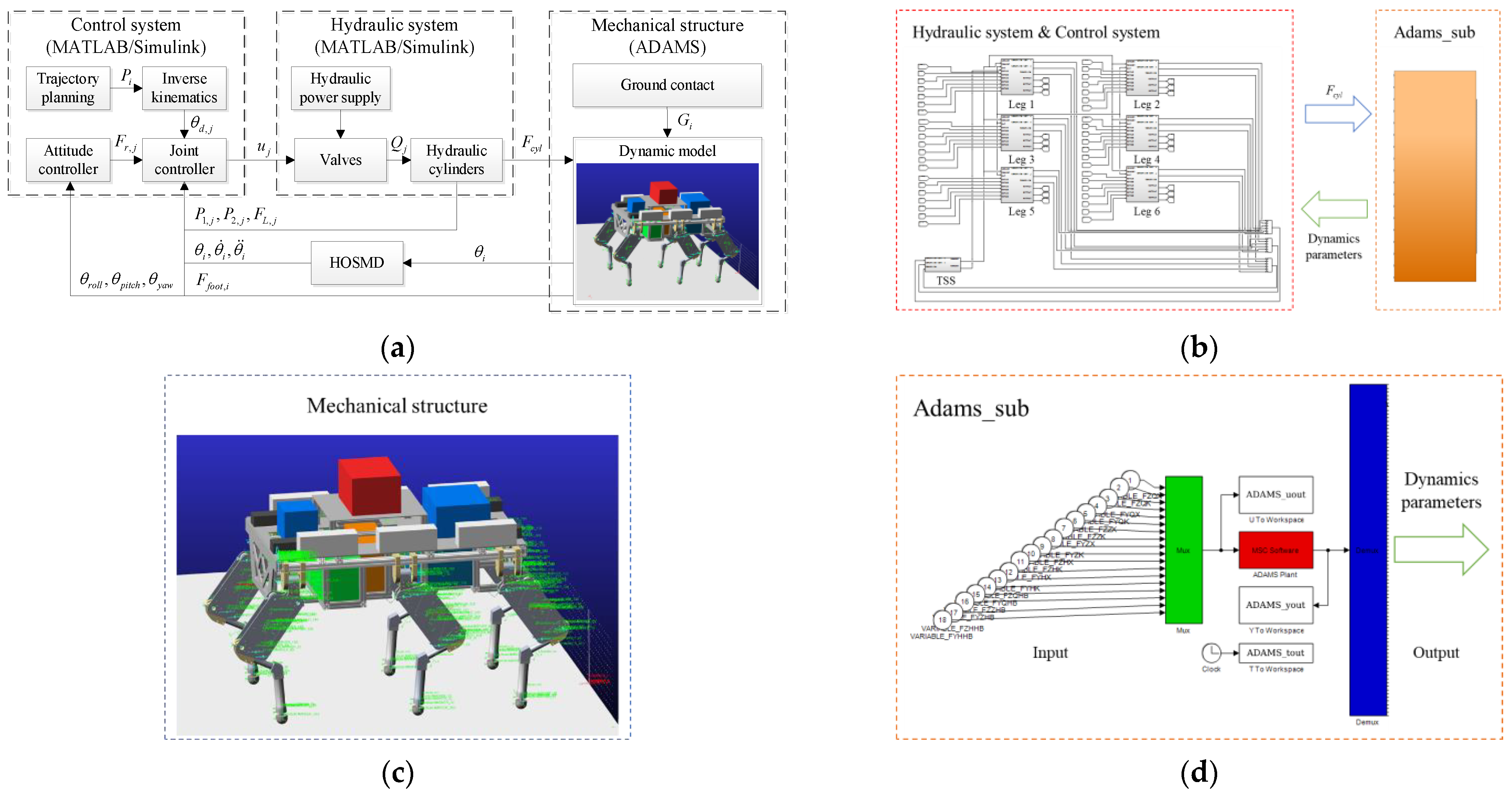
2.3. Control System Architecture

According to the characteristics of HHR, such as a large number of sensors, high real-time requirements, and complex complicated control strategy calculation, a hierarchical control system is established as Figure 3 depicts. Firstly, a remote personal computer (PC) works as an upper layer, which can provide an interactive interface and Wi-Fi communication. Secondly, an industrial personal computer PXIe-8861 behaves as the lower layer to complete gait planning, trajectory planning, control algorithm, and communication in the Wi-Fi module. Also, signal sampling and output can be implemented by the multifunction I/O module PXIe-6375 and output module PXIe-6739. Angle encoders are mounted in the joints to measure the joint angles, while force sensors and pressure gauges are used to measure the load force and hydraulic cylinders’ pressure. In addition, foot force sensors are mounted on the feet of HHR to measure the ground contact force to compensate for the model and distinguish whether the stance phase or swing phase. Finally, an inertial measurement unit (IMU) is fixed on the robot trunk to measure the attitude of the robot. The specifications of different sensors are shown in

Table 1. List of specifications of different sensors.

Sensor	Model	Input Range	Output Range	Resolution
Angular encoder	R22H	270°	0–5 V	0.0659°
Pressure	MIK-P300	0–25 MPa	0–5 V	-
Force	BSLM-3	0–20 kN	0–5 V	-
Foot force	CHHBM-1	0–500 kg	0–5 V	-
IMU	LPMS-RS232AL2	Roll: ±180°, Pitch: ±90°; Yaw: ±180°	-	-

.

3. System Modelling

3.1. Kinematics Modelling

Each leg of HHR adopts the same structure as the front left leg as Figure 4 shows. ${\mathrm{X}}_1$, ${\mathrm{X}}_2$, ${\mathrm{X}}_3$, ${\mathrm{X}}_4$ are the four hinge points connected to two hydraulic cylinders of the knee and hip joint. $c_0$, $c_1$, $c_2$ are the length of three hydraulic cylinders, respectively. $a_0$, $b_0$, $a_1$, $b_1$, $a_2$, $b_2$ are the mounting position of three hydraulic cylinders, respectively. ${\theta }_0$, ${\theta }_1$, ${\theta }_2$ are the joint angles of RAA, HFE, and KFE, respectively. $L_0$, $L_1$, $L_2$ are the length of the leg links, respectively, which will be used in kinematics models. $e_{11}$, $e_{12}$, $e_{21}$, $e_{22}$, $\phi$ are the auxiliary angles in the calculation.

The relationship between the length of hydraulic cylinders and the joint angles can be written as

$$\{\begin{array}{l}{c}_0=\sqrt{a_0{}^2+b_0{}^2+2a_0{b}_0\cos ({\theta }_0-e_{01}-e_{02})}=c_{00}+x_{pr}\\ c_1=\sqrt{a_1{}^2+b_1{}^2+2a_1{b}_1\cos ({\theta }_1-e_{11}+e_{12})}=c_{10}+x_{ph}\\ c_2=\sqrt{a_2{}^2+b_2{}^2+2a_2{b}_2\cos ({\theta }_2-e_{21}+e_{22}+\phi )}=c_{20}+x_{pk}\end{array}$$

(1)

$$\{\begin{array}{l}{l}_0=-\frac{a_0{b}_0\sin ({\theta }_0-e_{01}-e_{02})}{c_0}\\ l_1=-\frac{a_1{b}_1\sin ({\theta }_1-e_{11}+e_{12})}{c_1}\\ l_2=-\frac{a_2{b}_2\sin ({\theta }_2-e_{21}+e_{22}+\phi )}{c_2}\end{array}$$

(2)

where ${\theta }_0$, ${\theta }_1$ and ${\theta }_2$ are the root, hip, and knee joint angles, respectively; $l_0$, $l_1$ and $l_2$ are the arms of output force of hydraulic cylinders, respectively; $c_{00}$, $c_{10}$ and $c_{20}$ are the root, hip, and knee joint initial hydraulic cylinders’ length, respectively; $x_{pr}$, $x_{ph}$ and $x_{pk}$ are the root, hip, and knee joint hydraulic cylinders’ displacement, respectively.

The forward kinematics and inverse kinematics models are developed below:

$$P(\theta )=\left[\begin{array}{c}-L_1\sin {\theta }_1-L_2\sin ({\theta }_1+{\theta }_2)\\ (L_0+L_1\cos {\theta }_1+L_2\cos ({\theta }_1+{\theta }_2))\sin {\theta }_0\\ -(L_0+L_1\cos {\theta }_1+L_2\cos ({\theta }_1+{\theta }_2))\cos {\theta }_0\end{array}\right]=\left[\begin{array}{c}{P}_x\\ P_y\\ P_z\end{array}\right]$$

(3)

$$\{\begin{array}{l}{\theta }_0=-\arctan \left(\frac{P_y}{P_z}\right)\\ {\theta }_1=-\arccos \left(\frac{L_1{}^2-L_2{}^2+L^2+P_x{}^2}{2L_1\sqrt{L^2+P_x{}^2}}\right)-\arctan \left(\frac{P_x}{L}\right)\\ {\theta }_2=\pi -\arccos \left(\frac{L_1{}^2+L_2{}^2-L^2-P_x{}^2}{2L_1{L}_2}\right)\end{array}$$

(4)

where $P(\theta )$ is the foot position in the root coordinate system; $L=\sqrt{P_y{}^2+P_z{}^2}-L_0$.

3.2. Hydraulic System Modelling

Compared with the traditional valve-controlled cylinder system, the SMISMO control system can separate the controls of meter-in and meter-out orifices, which will increase the flexibility of the valve and the energy efficiency of the system. To simplify the hydraulic system, the hip joint can be taken as an example in Figure 5 and the following controller design is based on it. Figure 5 describes how the SMISMO control system works. $Q_{s1}$ and $Q_{s2}$ are the flow rate leaving from the low-pressure pump and the high-pressure pump, respectively. $Q_{a1}$ and $Q_{a2}$ are the flow rate leaving from the low-pressure accumulator and the high-pressure accumulator, respectively. In this SMISMO control system, valve $V_1$ can provide high-pressure oil, while the valve $V_2$ and $V_3$ can offer low-pressure oil. When the legs of HHR are in the stance phase or the swing phase, different valve configurations are proposed in Section 4.1 in detail.

Neglecting the leakage, the pressure dynamics of the cylinder chambers can be derived by

$$\frac{V_{h1}}{{\beta }_e}{\dot{P}}_{h1}=Q_{h1}-A_1{\dot{x}}_{ph}$$

(5)

$$\frac{V_{h2}}{{\beta }_e}{\dot{P}}_{h2}=-Q_{h2}+A_2{\dot{x}}_{ph}$$

(6)

where $V_{h1}=V_{h10}+A_1{x}_{ph}$, $V_{h2}=V_{h20}-A_2{x}_{ph}$, $V_{h1}$ and $V_{h2}$ are the hydraulic cylinder volume without the rod and with the rod; $V_{h10}$ is the volume of the cavity between the valves and the hydraulic cylinder without the rod in the initial position, $V_{h20}$ is the volume of the cavity between the valves and the hydraulic cylinder with the rod; $P_{h1}$ and $P_{h2}$ are the hydraulic cylinder pressure without rod and with the rod; $x_{ph}$ is the hydraulic cylinder displacement; $Q_{h1}$ is the flow entering into the cylinder chamber without the rod; $Q_{h2}$ is the flow leaving the cylinder chamber with the rod; $A_1$ and $A_2$ are the hydraulic cylinder areas without the rod and with the rod; ${\beta }_e$ is the bulk modulus of hydraulic oil.

The dynamics equation of SMISMO control valves can be written as below:

$$\frac{x_{vi}(s)}{u_i(s)}=\frac{{\omega }_v{}^2}{s^2+2\zeta {\omega }_{v}s+{\omega }_v{}^2}$$

(7)

where $x_{vi}$ is the displacement of the spool in SMISMO control valve; $u_i$ is the control voltage; ${\omega }_v$ is the natural frequency of the valve; $\zeta$ is the damping coefficient.

Ignoring the dynamics of the valves, the flow rate of SMISMO control valves can be depicted as below:

$$Q_{hv1}=\{\begin{array}{c}{K}_{qh}\cdot u_1\cdot \sqrt{P_{s2}-P_{h1}}\hspace{0.17em}{u}_1\ge 0\\ K_{qh}\cdot u_1\cdot \sqrt{P_{h1}-P_r}\hspace{0.17em}\hspace{0.17em}{u}_1<0\end{array}$$

(8)

$$Q_{hv2}=\{\begin{array}{c}{K}_{qh}\cdot u_2\cdot \sqrt{P_{s1}-P_{h1}}\hspace{0.17em}{u}_2\ge 0\\ K_{qh}\cdot u_2\cdot \sqrt{P_{h1}-P_r}\hspace{0.17em}\hspace{0.17em}{u}_2<0\end{array}$$

(9)

$$Q_{hv3}=\{\begin{array}{c}-K_{qh}\cdot u_3\cdot \sqrt{P_{s1}-P_{h2}}\hspace{0.17em}{u}_3\ge 0\\ -K_{qh}\cdot u_3\cdot \sqrt{P_{h2}-P_r}\hspace{0.17em}{u}_3<0\end{array}$$

(10)

$$\{\begin{array}{l}{Q}_{h1}=Q_{hv1}+Q_{hv2}\\ Q_{h2}=Q_{hv3}\end{array}$$

(11)

where $Q_{hv1}$, $Q_{hv2}$ and $Q_{hv3}$ are the flow rate of three directional control valves $V_1$, $V_2$ and $V_3$; $u_1$, $u_2$ and $u_3$ are the input voltage of valves $V_1$, $V_2$ and $V_3$; $P_{s1}$ is the low supply pressure; $P_{s2}$ is the high supply pressure; $P_r$ is oil tank pressure; $K_{qh}$ is the valve’s flow gain coefficient.

The dynamics model of hydraulic cylinder can be written as

$$F_{cyl}=A_1{P}_{h1}-A_2{P}_{h2}=M_h\cdot {\ddot{x}}_{ph}+B_p\cdot {\dot{x}}_{ph}+d$$

(12)

where $F_{cyl}$ is hydraulic cylinder output force; $M_h$ is mass load; $d=F_h+F_f$, $F_h$ is load force, $F_f$ is cylinder friction force; $B_p$ is the viscous coefficient.

4. Controller Design

In the HHR control system, the onboard industrial personal computer PXIe-8861 can obtain signals of joint angle, load force, hydraulic cylinder pressure, and foot force from different sensors, thus implementing the control algorithm to achieve the high-precision and steady locomotion of the robot. Combined with the SMISMO system as Figure 5 shows, all the valves need to be appropriately configured, not only to get better control performance but to save energy as well.

4.1. Valve Configuration in TSS

Three valves are configured as

Table 2. Valve configuration in different phases.

Phase	${\mathit{V}}_1$	${\mathit{V}}_2$	${\mathit{V}}_3$	Flow Rate
Stance phase	On	Off	On	$\begin{array}{l}{Q}_{h1}=Q_{hv1}\\ Q_{h2}=Q_{hv3}\end{array}$
Swing phase	Off	On	On	$\begin{array}{l}{Q}_{h1}=Q_{hv2}\\ Q_{h2}=Q_{hv3}\end{array}$

to deal with different load forces in the stance phase and swing phase. Owing to the foot force sensors installed on the robot feet, the foot force will be gained to easily distinguish which leg is in the stance phase. When the contact detection identifies that the leg is in the stance phase, the control voltage of $V_2$ will be set to zero, which will turn off $V_2$. In this case, $V_1$ and $V_3$ can independently control the flow rate of the chamber without the rod and with the rod, respectively, which will form a SMISMO control system automatically. $V_1$ is connected to the high-pressure resource $P_{s2}$, oil tank, and the chamber without the rod, while $V_3$ is connected to the low-pressure resource $P_{s1}$, oil tank, and the chamber with the rod. Through the control algorithm designed, the hydraulic cylinder can implement the exact trajectory tracking and periodic reciprocating motion. When the leg is in the swing phase, the control voltage of $V_1$ will be set to zero, which will turn off $V_1$. Thus, $V_2$ and $V_3$ will control the movement of the hydraulic cylinder. Because $V_2$ is connected to the low-pressure resource $P_{s1}$ instead of $P_{s2}$, energy in the hydraulic cylinder extension can be saved.

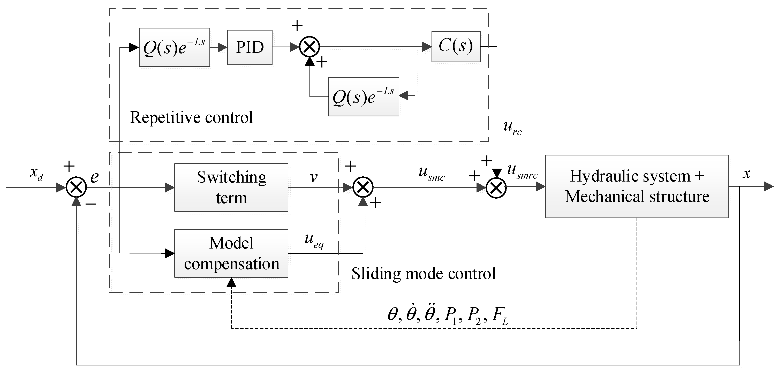
4.2. Sliding Mode Repetitive Control

Firstly, a sliding mode control (SMC) is proposed to realize joint angle control of HHR. Assuming the leg is in the stance phase, only $V_1$ and $V_3$ are, thus, working. From Equations (5), (6) and (12), we can easily get

$$\{\begin{array}{l}\frac{V_{h1}}{{\beta }_e}{\dot{P}}_{h1}=Q_{h1}-A_1{\dot{x}}_{ph}\\ \frac{V_{h2}}{{\beta }_e}{\dot{P}}_{h2}=-Q_{h2}+A_2{\dot{x}}_{ph}\\ F_{cyl}=M_h\cdot {\ddot{x}}_{ph}+B_p\cdot {\dot{x}}_{ph}+d\end{array}$$

(13)

where

$$\{\begin{array}{l}{Q}_{h1}=K_{qh}\cdot u_1\cdot \sqrt{\Delta P_1}\\ Q_{h2}=-K_{qh}\cdot u_3\cdot \sqrt{\Delta P_2}\end{array}$$

(14)

$$\begin{array}{l}\Delta P_1=\{\begin{array}{cc}{P}_{s2}-P_{h1}& u_1>0\\ P_{h1}-P_t& u_1<0\end{array}\\ \Delta P_2=\{\begin{array}{cc}{P}_{s1}-P_{h2}& u_3>0\\ P_{\mathrm{h}2}-P_t& u_3<0\end{array}\end{array}$$

(15)

Define a set of new parameters as

$$\{\begin{array}{l}{f}_1=-\frac{B_p}{M_h}{\dot{x}}_{ph}\\ g_1=\frac{1}{M_h}\\ f_2=-\left(\frac{A_1{}^2}{V_{h1}}+\frac{A_2{}^2}{V_{h2}}\right){\beta }_e{\dot{x}}_{ph}=f_{21}+f_{22}\\ g_2=\left(\frac{A_1}{V_{h1}}\sqrt{\Delta P_1}+\frac{A_2}{V_{h2}}\sqrt{\Delta P_2}\right){\beta }_e{K}_q=g_{21}+g_{22}\end{array}$$

(16)

where

$$\{\begin{array}{l}{f}_{21}=-\frac{A_1{}^2}{V_{h1}}{\beta }_e{\dot{x}}_{ph}\\ f_{22}=-\frac{A_2{}^2}{V_{h2}}{\beta }_e{\dot{x}}_{ph}\\ g_{21}=\frac{A_1}{V_{h1}}\sqrt{\Delta P_1}{\beta }_e{K}_{qh}\\ g_{22}=\frac{A_2}{V_{h2}}\sqrt{\Delta P_2}{\beta }_e{K}_{qh}\end{array}$$

(17)

The control voltage $u_1$ of $V_1$ can be calculated. Define state variables and establish state-space equations as

$$\{\begin{array}{l}{x}_1=x_{ph}\\ x_2={\dot{x}}_{ph}\\ x_3={\ddot{x}}_{ph}\\ x_4=F_{cyl}\end{array}$$

(18)

$$\{\begin{array}{l}{\dot{x}}_1=x_2\\ {\dot{x}}_2=g_1{x}_4+f_1-g_{1}d\\ {\dot{x}}_3=g_1(g_{21}{u}_1+f_{21}-A_2{\dot{P}}_{h2})+{\dot{f}}_1-g_1\dot{d}+\Delta \\ {\dot{x}}_4=g_{21}u+f_{21}-A_2{\dot{P}}_{h2}\end{array}$$

(19)

For simplicity, the following practical assumption is made.

Assumption 1.

The extent of parametric uncertainties and uncertain nonlinearities are known, i.e.,

$$\Delta \in {\mathsf{\Omega }}_{\Delta }\equiv \left\{\Delta :\left|\Delta (x,t)\right|\le \delta (x,t)\right\}$$

(20)

where$\Delta \in {\mathsf{\Omega }}_{\Delta }$is uncertain nonlinearity and other disturbance from environments, $\delta (x,t)$ is known.

Let

$$\{\begin{array}{l}{e}_0={\displaystyle \int (x_{ph}-x_d)}dt\\ e_1=x_{ph}-x_d\\ e_2={\dot{x}}_{ph}-{\dot{x}}_d\\ e_3={\ddot{x}}_{ph}-{\ddot{x}}_d\end{array}$$

(21)

where $x_d$ is the desired hydraulic cylinder displacement.

The sliding surface can be designed as

$$s=k_0{e}_0+k_1{e}_1+k_2{e}_2+e_3$$

(22)

where $k_0$, $k_1$, $k_2$, $k_3$ can be chosen such that $s^3+k_2{s}^2+k_{1}s+k_0$ is Hurwitz.

A positive semi-definite Lyapunov function can be written as

$$V_1=\frac{1}{2}{s}^2$$

(23)

The derivative $V_1$ can be expressed as

$${\dot{V}}_1=s[k_0{e}_1+k_1{e}_2+k_2{e}_3+g_1(g_{21}{u}_1+f_{21}-A_{h2}{\dot{P}}_{h2})+{\dot{f}}_1-g_1\dot{d}+\Delta -{\stackrel{⃛}{x}}_d]$$

(24)

The control input $u_1$ of valve $V_1$ can be designed as

$$u_1=u_{smc1}=u_{eq1}+v_1$$

(25)

where $u_{eq1}$ is feedback linearization compensation component, $v_1$ is a sliding mode switching component.

$$u_{eq1}=-\frac{1}{g_1{g}_{21}}(k_0{e}_1+k_1{e}_2+k_2{e}_3+g_1{f}_{21}-g_1{A}_2{\dot{P}}_2+{\dot{f}}_1-g_1\dot{d}-{\stackrel{⃛}{x}}_d)$$

(26)

$$v_1=-\frac{1}{g_1{g}_{21}}[k_{s1}s+{\rho }_{1}sat(\frac{s}{\epsilon })]$$

(27)

where $k_{s1}>0$ determines the exponential convergence speed of the error on the sliding surface; ${\rho }_1\ge {\rho }_{01}=\frac{\delta (x,t)}{g_1{g}_{21}}>0$; $sat(\cdot )$ is a high-slope saturation function which can replace the signum function to eliminate chattering, $\epsilon$ is the thickness of the boundary layer.

$$sat(\frac{s}{\epsilon })=\{\begin{array}{ll}1& s>\epsilon \\ \frac{s}{\epsilon }& \left|s\right|\le \epsilon \\ -1& s<-\epsilon \end{array}$$

(28)

Thus, when $\left|s\right|>\epsilon$

$${\dot{V}}_1=-k_{s1}{s}^2-{\rho }_1\left|s\right|+\Delta \cdot s\le -k_s{s}^2\le 0$$

(29)

The closed-loop system is stable according to Lasalle’s invariant principle.

Similarly, the control $u_3$ of valve $V_3$ can be designed as

$$u_3=u_{smc3}=u_{eq3}+v_3$$

(30)

where

$$u_{eq3}=\frac{1}{g_1{g}_{22}}(k_0{e}_1+k_1{e}_2+k_2{e}_3+g_1{f}_{22}+g_1{A}_1{\dot{P}}_1+{\dot{f}}_1-g_1\dot{d}-{\stackrel{⃛}{x}}_d)$$

(31)

$$v_3=\frac{1}{g_1{g}_{22}}[k_{s3}s+{\rho }_{3}sat(\frac{s}{\epsilon })],{\rho }_3\ge {\rho }_{03}=\frac{\delta (x,t)}{g_1{g}_{22}}>0$$

(32)

Secondly, the repetitive control (RC) will be combined with SMC to form SMRC to improve tracking accuracy. RC, based on the internal model principle, is regarded as a simple learning control because the control input is calculated using the information of the error signal in the preceding periods. RC is often utilized to track periodic signals, which can effectively suppress periodic load interference. The schematic of SMRC is illustrated in Figure 6.

$$u_{smrc}=u_{smc}+u_{rc}$$

(33)

where $u_{smc}$ is SMC output; $u_{rc}$ is RC output.

$$G_{rc}(s)=\frac{Q(s)e^{-Ls}{G}_{PID}(s)C(s)}{1-Q(s)e^{-Ls}}$$

(34)

where $G_{rc}(s)$ is the transfer function from position error $e$ to RC output $u_{rc}$; $Q(s)$ is the compensation term to ensure system stability, which is always chosen as a constant near 1 or a low-pass filter; $e^{-Ls}$ is time delay element, $L$ is the delay time; $G_{PID}(s)$ is the transfer function of a proportional-integral-derivative (PID) controller; $C(s)$ is the stabilization compensation term for amplitude and phase correction of the controller.

As a comparison, a conventional proportional-integral-derivative (PID) controller is designed as follows:

$$u_1=k_{p}e(t)+k_i{\displaystyle \int e(t)}dt+k_d\frac{de(t)}{dt}$$

(35)

where $e(t)$ is the tracking error; $k_p$, $k_i$, $k_d$ are the proportional gain, integral gain, and derivative gain, respectively.

4.3. High-Order Sliding Mode Differentiator

Although the joint angle can be obtained easily through the angle encoders, it is difficult to get the joint angular velocity, and acceleration for the direct differential will bring in and amplify noise. Thus, a high-order sliding mode differentiator (HOSMD) is proposed to gain accurate joint angular velocity and acceleration.

The HOSMD can be expressed as

$$\begin{array}{l}{\dot{z}}_0=v=z_1-k_{d0}{\left|z_0-f(t)\right|}^{2/3}sign(z_0-f(t))\\ {\dot{z}}_1=a=z_2-k_{d1}{\left|z_1-v\right|}^{1/2}sign(z_1-v)\\ {\dot{z}}_2=-k_{d2}\left|z_2-a\right|\end{array}$$

(36)

where $f(t)$ can be the joint angle $\theta$; $v$ is the calculated joint angular velocity; $a$ is the calculated joint angular acceleration; $k_{d0}$, $k_{d1}$, $k_{d2}$ are the designed parameters, respectively.

In order to prove the stability of HOSMD, the new parameters can be defined as ${\sigma }_i=(z_i-f^{(i)}(t))/L$, $k_{di}={\lambda }_i{L}^{1/(3-i)}$ $(i=0~2)$; thus, Equation (36) can be rewritten as

$$\begin{array}{l}{\dot{\sigma }}_0=-{\lambda }_0{\left|{\sigma }_0\right|}^{2/3}sign({\sigma }_0)+{\sigma }_1\\ {\dot{\sigma }}_1=-{\lambda }_1{\left|{\sigma }_1-{\dot{\sigma }}_0\right|}^{1/2}sign({\sigma }_1-{\dot{\sigma }}_0)+{\sigma }_2\\ {\dot{\sigma }}_2=-{\lambda }_{2}sign({\sigma }_1-{\dot{\sigma }}_0)-\epsilon \end{array}$$

(37)

where $\epsilon =\frac{f^{(3)}(t)}{L}\in [-1,1]$, $L>\left|f^{(3)}(t)\right|$ is a designed known Lipschitz constant; ${\lambda }_0$, ${\lambda }_1$, ${\lambda }_2$ are the designed parameters, respectively.

A positive semi-definite Lyapunov function can be written as

$$V=\frac{1}{2}{\sigma }_0{}^2+\frac{1}{2}{({\sigma }_1-{\dot{\sigma }}_0)}^2+\frac{1}{2}{({\sigma }_2-{\dot{\sigma }}_1)}^2$$

(38)

The derivative $V$ can be expressed as

$$\begin{array}{c}\dot{V}=-{\lambda }_0{\left|{\sigma }_0\right|}^{5/3}-{\lambda }_1{\left|{\sigma }_1-{\dot{\sigma }}_0\right|}^{3/2}-{\lambda }_2\left|{\sigma }_2-{\dot{\sigma }}_1\right|+{\sigma }_0{\sigma }_1\\ +({\sigma }_1-{\dot{\sigma }}_0)({\sigma }_2-{\ddot{\sigma }}_0)+({\sigma }_2-{\dot{\sigma }}_1)(-\epsilon -{\ddot{\sigma }}_1)\end{array}$$

(39)

when the parameters are chosen as

$$\begin{array}{l}{\lambda }_0>{\left|{\sigma }_0\right|}_{\max }^{2/3}{\left|{\sigma }_0\right|}_{\max }\\ {\lambda }_1>{\left|{\sigma }_1-{\dot{\sigma }}_0\right|}_{\max }^{-1/2}{\left|{\sigma }_2-{\ddot{\sigma }}_0\right|}_{\max }\\ {\lambda }_2>{\left|\epsilon +{\ddot{\sigma }}_1\right|}_{\max }\end{array}$$

(40)

Thus

$$\dot{V}<0$$

(41)

HOSMD can be stable. Through HOSMD and mechanical structure Equation (1), the joint angle, angular velocity, and acceleration can be straightforwardly calculated and transferred into the hydraulic cylinder’s displacement, which can be utilized in the SMRC algorithm.

5. Simulation and Analysis

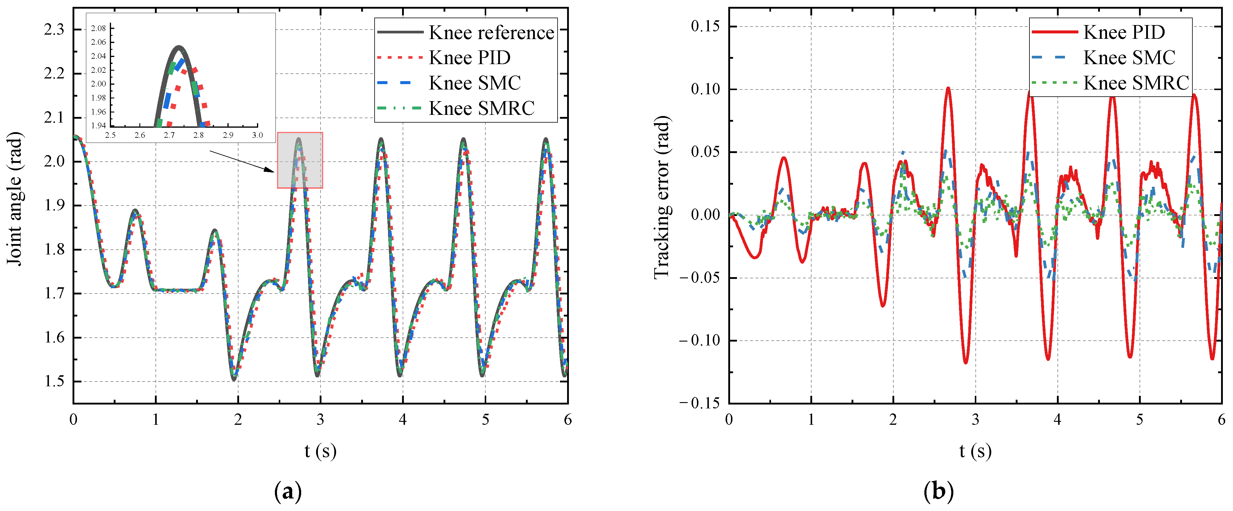
5.1. Joint Trajectory Tracking

The co-simulation model of HHR is built in both ADAMS and MATLAB/Simulink, as Figure 7 shows. The mechanical structure is established in ADAMS, while the hydraulic system and control system are established in MATLAB/Simulink. The interactive interface of ADAMS and MATLAB/Simulink can be packaged into an Adams_sub module, which can take the hydraulic cylinders’ force as inputs. Through the ground contact model established, ADAMS will return the dynamics parameters of HHR to MATLAB/Simulink, which will act as feedback in the control algorithm. The ground contact parameters set in the ADAMS are shown in

Table 3. Ground contact parameters in ADAMS.

Parameters	Value	Unit
Stiffness	$2.855\times {10}^6$	$\mathrm{N}/\mathrm{m}$
Force exponent	2.2	-
Damping	$1\times {10}^6$	$\mathrm{N}/(\mathrm{m}/\mathrm{s})$
Penetration depth	$1\times {10}^{-4}$	m
Static coefficient	0.7	-
Dynamic coefficient	0.55	-
Stiction transition velocity	0.1	$\mathrm{m}/\mathrm{s}$
Friction transition velocity	10	$\mathrm{m}/\mathrm{s}$

, which are vital to the co-simulation.

The foot trajectory with a duty factor $\beta =0.5$ (the fraction of a cycle time when the leg is in the stance phase) can be described as follows, and the curve is shown in Figure 8.

$$\{\begin{array}{l}{P}_{x,sw}(t)=\left(a_6{t}^6+a_5{t}^5+a_4{t}^4+a_3{t}^3+a_2{t}^2+a_{1}t+a_0\right)S+s_i\\ P_{z,sw}(t)=\left(b_6{t}^6+b_5{t}^5+b_4{t}^4+b_3{t}^3+b_2{t}^2+b_{1}t+b_0\right)w-H_0\\ P_{x,st}(t)=\left(\frac{3}{2}-\frac{2t}{T}\right)S+s_i\\ P_{z,st}(t)=-H_0\end{array}$$

(42)

where $P_{x,sw}(t)$, $P_{z,sw}(t)$, $P_{x,st}(t)$ and $P_{z,st}(t)$ are foot position in the swing phase and stance phase, respectively; $S$, $s_i$, $w$, $H_0$ and $T$ are the step length, offset, step height, and the cycle of the gait, respectively; $a_i$ and $b_i$ $(i=1~6)$ are the designed six-order polynomial parameters through the constraints in

Table 4. Position, velocity, and acceleration constraints in foot trajectory.

Constraints	X Direction	Z Direction
$P_{x/z}(0)$	$-S/2+s_i$	$-H_0$
$P_{x/z}(T/4)$	$s_i$	$-H_0+w$
$P_{x/z}(T/2)$	$S/2+s_i$	$-H_0$
${\dot{P}}_{x/z}(0)$	$-S/T$	0
${\dot{P}}_{x/z}(T/2)$	$-S/T$	0
${\ddot{P}}_{x/z}(0)$	0	0
${\ddot{P}}_{x/z}(T/2)$	0	0

.

HHR can walk in a tripod gait at 0.75 m/s, whose cycle is 1 s. The main parameters of the system and controllers in the hip joint implemented in the simulation are shown in

Table 5. System parameters in the simulation.

Parameters	Value	Unit
$V_{h10}$	$2.8061\times {10}^{-5}$	${\mathrm{m}}^3$
$V_{h20}$	$5.1819\times {10}^{-5}$	${\mathrm{m}}^3$
$A_1$	0.0013	${\mathrm{m}}^2$
$A_2$	$7.6577\times {10}^{-4}$	${\mathrm{m}}^2$
${\beta }_e$	$7\times {10}^8$	${\mathrm{N}/\mathrm{m}}^2$
$M_h$	50	kg
$B_p$	2000	$\mathrm{N}/(\mathrm{m}/\mathrm{s})$
$K_{qh}$	$3.5635\times {10}^{-7}$	${\mathrm{m}}^3/(\mathrm{s}\cdot {\mathrm{Pa}}^{\frac{1}{2}})$
${\omega }_v$	439.823	rad/s
$\zeta$	0.707	-

and

Table 6. Main parameters of controllers in the hip joint.

Controller	Gain	Value
PID	$k_p$	50
	$k_i$	1
	$k_d$	0.001
SMRC	$k_0$	50
	$k_1$	0.3
	$k_2$	0.001
	$k_{s1}$	0.01
	${\rho }_1$	0.1
	$\epsilon$	10
	$Q(s)$	0.95

. As for the SMRC, there’re two procedures to implement the controller tuning. Firstly, the SMC controller is established according to the joint hydraulic model. The SMC controller is similar to a PD controller with other feedback linearization model compensation terms. Then, when the parameters of SMC controller are tuned, an RC controller is added to form a SRMC controller and improve the performance of joint trajectory tracking. Figure 9 shows the different control performances in joint angles through PID, SMC, and SMRC controllers while velocity and acceleration of the knee and hip can be obtained through HOSMD, as Figure 10 shows. The tracking error analysis is illustrated in detail in

Table 7. Tracking error analysis.

Control Strategy	$\left|{\mathit{e}}_{\mathbf{m}\mathbf{a}\mathbf{x}}\right| \left(\mathbf{rad}\right)$		${\mathit{e}}_{\mathbf{R}\mathbf{M}\mathbf{S}} \left(\mathbf{rad}\right)$
	${\mathit{\theta }}_1 \left(\mathbf{rad}\right)$	${\mathit{\theta }}_2 \left(\mathbf{rad}\right)$	${\mathit{\theta }}_1 \left(\mathbf{rad}\right)$	${\mathit{\theta }}_2 \left(\mathbf{rad}\right)$
PID	0.141	0.118	0.043	0.046
SMC	0.092	0.054	0.027	0.022
SMRC	0.057	0.043	0.015	0.012

. It’s obvious that with the control of SMRC, the absolute maximum tracking error of hip and knee decreases to 0.057 rad and 0.043 rad compared with PID, which are reduced by 59.58% and 63.53%, respectively. Furthermore, the root mean square (RMS) tracking error can also be reduced by 65.64% and 74.74%, respectively, which brings about great improvement.

5.2. Energy Consumption Analysis

HHR usually implements a tripod gait, which means there’re always three legs in the stance phase to support the robot trunk ideally. The hydraulic cylinder output force is shown in Figure 11. Taking a gait cycle (2–3 s) as an example, legs in the stance phase (2–2.5 s) need a rather large force to support the robot trunk and provide dynamic movement. However, in the swing phase (2.5–3 s), a small driving force is required because the hydraulic cylinders only need to provide output force to drive the legs to complete the swing motion, whose mass is rather small. On the contrary, from Figure 8, legs in the swing phase have a longer movement distance compared with those in the stance phase, which means more flow rate is required. As a result, a TSS system is designed with a high-pressure pump and a low-pressure pump, which provide a hydraulic resource for legs in the swing phase and stance phase, respectively.

The system energy consumption of OSS and TSS can be calculated, respectively, as follows:

$$E_{OSS}={\displaystyle {\int }_0^T{P}_{OSS}}dt={\displaystyle {\int }_0^T{P}_s{Q}_s}dt$$

(43)

$$E_{TSS}={\displaystyle {\int }_0^T{P}_{TSS}}dt={\displaystyle {\int }_0^{T_1}{P}_{s1}{Q}_{s1}}dt+{\displaystyle {\int }_0^{T_2}{P}_{s2}{Q}_{s2}}dt$$

(44)

$$T=T_1+T_2$$

(45)

$$\eta =\frac{E_{OSS}-E_{TSS}}{E_{OSS}}\times 100\%$$

(46)

where $P_{OSS}$ and $Q_{TSS}$ are the instantaneous system output power in OSS, respectively; $P_s$ and $Q_s$ are the system pressure and flow rate in OSS, respectively; $P_{s1}$ and $P_{s2}$ are the pressure of the low supply pressure and the high supply pressure in TSS, respectively; $Q_{s1}$ and $Q_{s2}$ are the flow rates which are supplied by the low-pressure and high-pressure source in TSS, respectively; $T_1$ and $T_2$ are the energy supply time by the low-pressure and high-pressure source during a gait cycle $T$; $\eta$ is the energy-saving efficiency.

The pressure and flow rate of OSS and TSS are shown in Figure 12. OSS provides a high system pressure of 18 MPa, while TSS supplies a high pressure of 18 MPa as well as a low pressure of 6 MPa. The average flow rate of $Q_s$ is $0.0012 {\mathrm{m}}^3/\mathrm{s}$, while the average flow rate of $Q_{s1}$ and $Q_{s2}$ are $9.9154\times {10}^{-4} {\mathrm{m}}^3/\mathrm{s}$ and $2.1583\times {10}^{-4} {\mathrm{m}}^3/\mathrm{s}$, respectively. Owing to the utilization of TSS, energy consumption can be greatly reduced. Figure 13 depicts the comparison of the instantaneous output power and energy consumption of OSS and TSS in a gait cycle of 1 s. With the configuration of valves in Table 2, the energy of legs in the swing phase can be saved. The simulation result shows that the energy consumption of OSS and TSS in a gait cycle (1 s) are 26.15 kJ and 12.57 kJ, respectively, which means TSS can achieve an energy-saving of 51.94% in HRR.

6. Conclusions

In this paper, the system design and control strategies of a HHR ZJUHEX01 with a two-stage supply pressure system (TSS) are introduced in detail. An overview of the mechanical system, hydraulic system, and control system is given, as well as the kinematics model and hydraulic system model. A SMRC controller for SMISMO hydraulic TSS system is proposed to help HHR get better control performance compared with the conventional PID, and the absolute maximum tracking error of hip and knee can be reduced by 59.58% and 63.53%, respectively. Also, the RMS tracking error of the hip and knee can be reduced by 65.64% and 74.74%, respectively, which brings about great improvement. Apart from that, a HOSMD is designed to get the joint angular velocity and acceleration for the use of the control algorithm. In the co-simulation model of ADAMS and MATLAB/Simulink, HHR can walk at a speed of 0.75 m/s in a tripod gait, where the effectiveness of the control strategy is also verified. Additionally, the energy consumption of TSS is compared with that of OSS to show a great energy-saving effect of 51.94%.

Although SRMC has a better performance in joint trajectory tracking than the conventional PID controller, it does not consider compliance when the feet are in contact with the ground. Thus, active compliance control, such as impedance control and virtual model control (VMC), is the research focus. Furthermore, based on the proposed SMISMO hydraulic TSS system, other energy-saving strategies can also be implemented. Future work will concentrate on the experiments of the active compliance control and energy-saving strategies in the HHR.

References

1. Suzumori, K.; Faudzi, A.A. Trends in hydraulic actuators and components in legged and tough robots: A review. Adv. Robot. 2018, 32, 458–476. [Google Scholar] [CrossRef]
2. He, J.; Gao, F. Mechanism, actuation, perception, and control of highly dynamic multilegged robots: A review. Chin. J. Mech. Eng. 2020, 33, 1–30. [Google Scholar] [CrossRef]
3. Tedeschi, F.; Carbone, G. Design issues for hexapod walking robots. Robotics 2014, 3, 181–206. [Google Scholar] [CrossRef] [Green Version]
4. Raibert, M.; Blankespoor, K.; Nelson, G.; Playter, R. BigDog, the rough-terrain quadruped robot. IFAC Proc. Vol. 2008, 41, 10822–10825. [Google Scholar] [CrossRef] [Green Version]
5. Semini, C.; Tsagarakis, N.G.; Guglielmino, E.; Focchi, M.; Cannella, F.; Caldwell, D.G. Design of HyQ—A hydraulically and electrically actuated quadruped robot. Proc. Inst. Mech. Eng. Part I J. Syst. Control Eng. 2011, 225, 831–849. [Google Scholar] [CrossRef]
6. Khan, H.; Kitano, S.; Frigerio, M.; Camurri, M.; Barasuol, V.; Featherstone, R.; Caldwell, D.G.; Semini, C. Development of the lightweight hydraulic quadruped robot—Minihyq. In Proceedings of the 2015 IEEE International Conference on Technologies for Practical Robot Applications (TePRA), Boston, MA, USA, 11–12 May 2015. [Google Scholar]
7. Semini, C.; Barasuol, V.; Goldsmith, J.; Frigerio, M.; Focchi, M.; Gao, Y.; Caldwell, D.G. Design of the hydraulically actuated, torque-controlled quadruped robot hyq2max. IEEE/ASME Trans. Mechatron. 2017, 22, 635–646. [Google Scholar] [CrossRef]
8. Jungsan, C.; Jin Tak, K.; Sangdeok, P.; Youngsoo, L.; Kabil, K. Jinpoong, posture control for the external force. In Proceedings of the IEEE ISR 2013, Seoul, Korea, 24–26 October 2013. [Google Scholar]
9. Rong, X.; Li, Y.; Ruan, J.; Li, B. Design and simulation for a hydraulic actuated quadruped robot. J. Mech. Sci. Technol. 2012, 26, 1171–1177. [Google Scholar] [CrossRef]
10. Chen, T.; Rong, X.; Li, Y.; Ding, C.; Chai, H.; Zhou, L. A compliant control method for robust trot motion of hydraulic actuated quadruped robot. Int. J. Adv. Robot. Syst. 2018, 15, 1729881418813235. [Google Scholar] [CrossRef] [Green Version]
11. Yang, K.; Zhou, L.; Rong, X.; Li, Y. Onboard hydraulic system controller design for quadruped robot driven by gasoline engine. Mechatronics 2018, 52, 36–48. [Google Scholar] [CrossRef]
12. Chen, X.; Gao, F.; Qi, C.; Tian, X.; Zhang, J. Spring parameters design for the new hydraulic actuated quadruped robot. J. Mech. Robot. 2014, 6, 021003. [Google Scholar] [CrossRef]
13. Li, M.; Jiang, Z.; Wang, P.; Sun, L.; Ge, S.S. Control of a quadruped robot with bionic springy legs in trotting gait. J. Bionic Eng. 2014, 11, 188–198. [Google Scholar] [CrossRef]
14. Chen, C.; An, H.; Wang, J.; Ma, H.; Wei, Q. Velocity control for trotting of a nudt quadruped robot. In Proceedings of the 2016 IEEE Chinese Guidance, Navigation and Control Conference (CGNCC), Nanjing, China, 12–14 August 2016. [Google Scholar]
15. Junyao, G.; Xingguang, D.; Qiang, H.; Huaxin, L.; Zhe, X.; Yi, L.; Xin, L.; Wentao, S. The research of hydraulic quadruped bionic robot design. In Proceedings of the 2013 ICME International Conference on Complex Medical Engineering, Beijing, China, 25–28 May 2013. [Google Scholar]
16. Barai, R.K.; Nonami, K. Robust adaptive fuzzy control law for locomotion control of a hexapod robot actuated by hydraulic actuators with dead zone. In Proceedings of the 2006 IEEE/RSJ International Conference on Intelligent Robots and Systems, Beijing, China, 9–15 October 2006. [Google Scholar]
17. Irawan, A.; Nonami, K. Optimal impedance control based on body inertia for a hydraulically driven hexapod robot walking on uneven and extremely soft terrain. J. Field Robot. 2011, 28, 690–713. [Google Scholar] [CrossRef]
18. Davliakos, I.; Roditis, I.; Lika, K.; Breki, C.-M.; Papadopoulos, E. Design, development, and control of a tough electrohydraulic hexapod robot for subsea operations. Adv. Robot. 2018, 32, 477–499. [Google Scholar] [CrossRef]
19. Tong, Z.; Ye, Z.; Gao, H.; He, J.; Deng, Z. Electro-hydraulic control system and frequency analysis for a hydraulically driven six-legged robot. In Proceedings of the 2016 IEEE International Conference on Aircraft Utility Systems (AUS), Beijing, China, 10–12 October 2016. [Google Scholar]
20. Cunha, T.B.; Semini, C.; Guglielmino, E.; De Negri, V.J.; Yang, Y.; Caldwell, D.G. Gain scheduling control for the hydraulic actuation of the hyq robot leg. In Proceedings of the COBEM, Gramado, Brazil, 15–20 November 2009. [Google Scholar]
21. Focchi, M.; Guglielmino, E.; Semini, C.; Boaventura, T.; Yang, Y.; Caldwell, D.G. Control of a hydraulically-actuated quad-ruped robot leg. In Proceedings of the 2010 IEEE International Conference on Robotics and Automation, Anchorage, AK, USA, 3–7 May 2010. [Google Scholar]
22. Bin, C.; Zhongcai, P.; Zhiyong, T. Self-tuning fuzzy-pid control for hydraulic quadruped robot. J. Harbin Inst. Technol. 2016, 48, 140–144. [Google Scholar]
23. Ke, X.; Lin, L.; Qing, W.; Hongxu, M. Design of single leg foot force controller for hydraulic actuated quadruped robot based on adrc. In Proceedings of the 2015 34th Chinese Control Conference (CCC), Hangzhou, China, 28–30 July 2015. [Google Scholar]
24. Barai, R.K.; Nonami, K. Locomotion control of a hydraulically actuated hexapod robot by robust adaptive fuzzy control with self-tuned adaptation gain and dead zone fuzzy pre-compensation. J. Intell. Robot. Syst. 2008, 53, 35–56. [Google Scholar] [CrossRef]
25. Wei, S.; Sun, C. Robust adaptive dynamic surface control for hydraulic quadruped robot hip joint. Trans. Beijing Inst. Technol. 2016, 36, 599–604. [Google Scholar]
26. Wang, C.; Li, Y.; Ruan, J.; Rong, X. Fuzzy sliding mode control of hydraulic cylinders driving a quadruped robot. In Proceedings of the 2010 8th World Congress on Intelligent Control and Automation, Jinan, China, 7–9 July 2010. [Google Scholar]
27. Quan, L.; Wei, Z.; Yu, B.; Liang, H. Decoupling control research on test system of hydraulic drive unit of quadruped robot based on diagonal matrix method. Intell. Control Autom. 2013, 04, 287–292. [Google Scholar] [CrossRef] [Green Version]
28. Gao, B.; Han, W. Neural network model reference decoupling control for single leg joint of hydraulic quadruped robot. Assem. Autom. 2018, 38, 465–475. [Google Scholar] [CrossRef]
29. Liu, Z.; Zhang, C.; Jin, B.; Zhai, S.; Dong, J. Design and development of an embedded controller for a hydraulic walking robot WLBOT. Appl. Sci. 2021, 11, 5335. [Google Scholar] [CrossRef]
30. Seok, S.; Wang, A.; Meng Yee, C.; Otten, D.; Lang, J.; Kim, S. Design principles for highly efficient quadrupeds and implementation on the mit cheetah robot. In Proceedings of the 2013 IEEE International Conference on Robotics and Automation, Karlsruhe, Germany, 6–10 May 2013. [Google Scholar]
31. Zhai, S.; Jin, B.; Cheng, Y. Mechanical design and gait optimization of hydraulic hexapod robot based on energy conservation. Appl. Sci. 2020, 10, 3884. [Google Scholar] [CrossRef]
32. Barasuol, V.; Villarreal-Magaña, O.A.; Sangiah, D.; Frigerio, M.; Baker, M.; Morgan, R.; Medrano-Cerda, G.A.; Caldwell, D.G.; Semini, C. Highly-integrated hydraulic smart actuators and smart manifolds for high-bandwidth force control. Front. Robot. AI 2018, 5, 51. [Google Scholar] [CrossRef] [PubMed] [Green Version]
33. Hua, Z.; Rong, X.; Li, Y.; Chai, H.; Li, B.; Zhang, S. Analysis and verification on energy consumption of the quadruped robot with passive compliant hydraulic servo actuator. Appl. Sci. 2020, 10, 340. [Google Scholar] [CrossRef] [Green Version]
34. Dong, J.; Jin, B.; Zhai, S.; Liu, Z.; Cheng, Y. Planning and analysis of centroid fluctuation gait for hydraulic hexapod robot. IEEE Access 2021, 9, 63538–63549. [Google Scholar] [CrossRef]
35. Yang, K.; Li, Y.; Zhou, L.; Rong, X. Energy efficient foot trajectory of trot motion for hydraulic quadruped robot. Energies 2019, 12, 2514. [Google Scholar] [CrossRef] [Green Version]
36. Deng, Z.; Liu, Y.; Ding, L.; Gao, H.; Yu, H.; Liu, Z. Motion planning and simulation verification of a hydraulic hexapod robot based on reducing energy/flow consumption. J. Mech. Sci. Technol. 2015, 29, 4427–4436. [Google Scholar] [CrossRef]
37. Tani, K.; Nabae, H.; Hirota, Y.; Endo, G.; Suzumori, K. Walking trajectory design of hydraulic legged robot with limited powered pump. In Proceedings of the 2021 IEEE International Conference on Robotics and Automation (ICRA), Xi’an, China, 30 May–5 June 2021. [Google Scholar]
38. Guglielmino, E.; Semini, C.; Yang, Y.; Caldwell, D.; Kogler, H.; Scheidl, R. Energy efficient fluid power in autonomous legged robotics. In Proceedings of the Dynamic Systems and Control Conference, Hollywood, CA, USA, 12–14 October 2009. [Google Scholar]
39. Xue, Y.; Yang, J.; Shang, J.; Wang, Z. Energy efficient fluid power in autonomous legged robotics based on bionic multi-stage energy supply. Adv. Robot. 2014, 28, 1445–1457. [Google Scholar] [CrossRef]
Figure 1. The hydraulic hexapod robot ZJUHEX01.
Machines 10 00305 g001
Figure 2. Schematic of the two-stage supply pressure hydraulic system (TSS).
Machines 10 00305 g002
Figure 3. Configuration of HHR control system.
Machines 10 00305 g003
Figure 4. Leg stretch with the definition of the leg geometry ( L 0 , L 1 , L 2 ), the cylinder mounting position ( a 0 , b 0 , a 1 , b 1 , a 2 , b 2 , e 11 , e 12 , e 21 , e 22 , φ ), the cylinder length ( c 0 , c 1 , c 2 ), joint angles ( θ 0 , θ 1 , θ 2 ), and labels of three leg joints, RAA: root abduction/adduction, HFE: hip flexion/extension, KFE: knee flexion/extension: (a) KFE and HFE; (b) RAA.
Machines 10 00305 g004
Figure 5. Schematic of the simplified hip joint SMISMO system.
Machines 10 00305 g005
Figure 6. The block diagram of SMRC.
Machines 10 00305 g006
Figure 7. ADAMS and MATLAB co-simulation model: (a) The block diagram of the co-simulation model; (b) The interactive interface of ADAMS and MATLAB/Simulink; (c) The mechanical structure of HHR in ADAMS; (d) Adams_sub module in MATLAB/Simulink.
Machines 10 00305 g007
Figure 8. Foot trajectory curve of HHR.
Machines 10 00305 g008
Figure 9. Comparison of PID, SMC, and SMRC in joint trajectory tracking and error: (a) Knee trajectory; (b) Knee tracking error; (c) Hip trajectory; (d) Hip tracking error.
Machines 10 00305 g009aMachines 10 00305 g009b
Figure 10. The velocity and acceleration of knee and hip through HOSMD: (a) Knee and hip angular velocity; (b) Knee and hip angular acceleration.
Machines 10 00305 g010
Figure 11. Hydraulic cylinder output force.
Machines 10 00305 g011
Figure 12. Pressure and flow rate of OSS and TSS: (a) Pressure of OSS and TSS; (b) Flow rate of OSS and TSS.
Machines 10 00305 g012
Figure 13. The instantaneous output power and energy consumption of OSS and TSS in a gait cycle: (a) The instantaneous output power of OSS and TSS; (b) Energy consumption of OSS and TSS.
Machines 10 00305 g013