Abstract
In this paper, a deep learning fault detection and prediction framework combining principal component analysis (PCA) and Informer is proposed to solve the problem of online monitoring of nuclear power valves which is hard to implement. More specifically, PCA plays the role of dimensionality reduction and fault feature extraction. It maps data with multi-dimensional space to low-dimensional space and extracts the main features. At the same time, the T-square and Q statistic thresholds are also provided to realize abnormal status monitoring. Meanwhile, Informer is a long-term series prediction method. It encrypts and decrypts data through the encoder and decoder to train a prediction model. Through the training of fault data, fault prediction can be realized. Experiments based on the sound waves collected from real valves can be continued, which also illustrates the effectiveness of the PCA–Informer model for fault diagnosis and fault prediction of nuclear power valves. Therefore, the online monitoring and maintenance of nuclear valves and other important equipment, without shutting down the nuclear station, can be achieved.
1. Introduction
The aging and wear of nuclear power valves has become a very common problem in the field of nuclear power fault diagnosis, which is attributed to the continuous opening and closing of the valves. Therefore, online monitoring of the failure status of nuclear power valves and failure prediction is very necessary, especially in such a special environment with a high radiation of nuclear power. By monitoring early indicators of failure prospectively, emerging problems can be identified before they become more widespread, thus playing an import role for industrial systems [1,2].
In addition to that, as many industrial managers are paying more attention to predictive maintenance, which is an important way to increase productivity while keeping the cost at a lower level, the fault prediction method is another rising hot topic [3]. Especially in the circumstance of the nuclear power unit, regular maintenance can only be carried out when lockout is taken, which is very time consuming and causes a waste of nuclear equipment. Fault diagnosis and prediction with high accuracy can be an efficient precaution.
In general, fault diagnosis methods have four classifications which are model-based, signal-based, knowledge-based, and hybrid/active methods [4]. Due to the rapid developments in network technologies, many engineering systems, especially the valve in the hydraulic system of safety-critical manufacturing systems, have created a large volume of historic data. Therefore, the fault model is easily established by the knowledge-based methods without the primary known models or signal patterns [5,6]. The advantage of this method is that it does not require any initial hypotheses about the relationship of input variables with the output; in addition, it is a method that does not rely on explicit models or signal symptoms. Generally, the methods of dealing with valve fault diagnosis problems are model-based approaches and sensor-based approaches [7,8,9]. In particular, internal leakage and friction in the valves are the most studied, widely expressed, and most represented valve faults [10,11,12]. In the beginning, the benchmark system was proposed, based on an in-depth study of the phenomena that can lead to potential faults in valve actuator systems. However, data-driven methods require less hypotheses [13,14]. Machine learning is one of the import methods for data-driven fault diagnosis, where information entropy is flexible and tolerant to the non-linearity problem, and is applied to analyze the characteristics of the signals.
Artificial neural network (ANN) is one of the most effective fault diagnosis methods. Two ANNs were used to classify eleven faulty types, such as the closed manual pressure valve, and normal models in seven or eight categories at the best vigilance values [15]. Later, a combination method for the fault detection of compressor valves based on basis pursuit (BP), wave matching, and Support vector machines (SVM) is presented [16]. A feedforward neural network was applied in the laser welding process monitoring and defects diagnosis [17]. However, ANNs are unable to generate discriminative features of faults and should be combined with feature extraction [18]. The feature extraction process is a conundrum and greatly impacts the result. In some of the recent literature, machine learning methods are unable to generate discriminative features of raw data and are always combined with the signal features extraction process [19,20].
Furthermore, prediction methods based on a deep learning structure is becoming a popular solution. In addition, it is a fully data-driven learning method that does not rely on rules-based programming. Except for these conventional machine learning algorithms, deep learning, a branch of machine learning, has been applied to many industrial applications, such as object identification and process monitoring, among others [21]. The proposed system adopted the machine learning approach, which learns the collected data and improves the prediction performance. New sensor technologies integrate machine learning, deep learning [22], and artificial intelligence [23] for structural health monitoring and sensor fault detection [24,25].
Models based on attention mechanisms are becoming popular in fault prediction. For example, the transformer is a new kind of neural architecture which encodes the input data as powerful features, and then calculates both representations and their relationship [26,27]. Latterly, Informer is a newly developed prediction model based on the transformer, which is quite suitable for long sequence time-series forecasting [28]. Many other variations are presented, such as the Reformer [29], Sparse Transformer [30], Longformer [31], and Performer [32], among others [33,34,35]. Many of these aforementioned models have been applied in natural language processing and prediction, sequence functions, image processing, and many other applications.
This paper proposes a PCA–Informer model for operation fault detection and prediction of nuclear valves to solve the problem of monitoring long time series. PCA is, first, applied to extract the fault features of sound and vibration signals, and the T2 and Q statistics are calculated. Then, a deep learning model, based on Informer, is further applied to predict the likely fault of the variable worth paying attention to. The Informer mechanism, with a temporal attention encoder and a decoder, is used to realize fault prediction. In our early work, PCA and its variations, such as recursive PCA and model-based PCA, were successfully applied in electric power grid status monitoring and islanding detection [36,37,38]. However, without the deep learning method, the traditional method and its extensions are not exceptionally accurate, especially in situations of noisy data and small samples.
2. Theories and Methods
2.1. Valve Leakage Acoustic Signals
Acoustic signals, also called acoustic emission (AE), is defined as the transient elastic waves generated by the rapid release of energy from localized sources. The AE technique is a nondestructive testing and monitoring method of mechanical parts through the detecting and analyzing of signals. It has been found that AE signals can be produced by fluid leakage and other working status, such as cracking, rubbing, polishing, impacting, and cavitations. Therefore, abnormal working conditions can also be revealed by AE signals. The frequency varies from 100 kHz to 1 MHz, and it can be easily identified by environmental noise from the factory. In the case of internal leakage in liquid valves, the generation of pseudo source produced AE signals, which were largely attributed to the turbulence induced by the internal leakage.
Popular processing techniques for AE signals are wavelet transform, spectrum analysis, and neural networks. In this paper, a data-driven method is proposed to combine PCA and deep learning models for clustering and the prediction of fault conditions. Before this, for the purpose of characteristic extraction, time domain and frequency domain analysis are needed. When check valves work under normal conditions, the signals detected are mainly background noise, which has small magnitude and behaves stably. When leakage occurs, a sudden change in signal amplitude will appear, which is attributed to the turbulence induced by the internal leakage. The root-mean-square (RMS) value is often used to calculate the average energy contained in the raw AE signals. Assuming an AE signal as a total number of K samples, its RMS value is provided by:
In order to effectively deal with noisy data and retain the overall and local important features of the original data, it is necessary to extract features from the original time-series acoustic signal before applying PCA. Frequency domain analysis can convert the original intractable time-domain signal into an easily analyzed frequency-domain signal. For frequency-domain analysis, the Fourier transform is always the first choice, through which the peak frequency, magnitude of the dominant frequency component, and the energy contained within the frequency band and other parameters can all be revealed. Usually, the power spectral density represents the distribution of the signal power over frequencies, which can be calculated as follows:
where P[m] is the power spectral density, X[m] is the discreate Fourier transform of an AE signal, and T is the sampling period. According to Parseval’s theorem, an equation can be rearranged and yielded:
ΔF = 1/(NT) represents the discrete frequency sample interval. P[m] is the average power of the signal measured in the time domain.
2.2. Valve Leakage Represented by AE Signals
The valve internal leakage fault can be simulated by the manual valve rotation method, which is commonly used by many researchers. The AE signals of working valves under well-sealed and leakage conditions are shown as Figure 1.

Figure 1.
AE signal waveform under valve well−sealed normal conditions and leakage: (a) normal state and (b) leaked state.
As evident from the time domain waveform in Figure 1, the horizontal axis represents time in s and the vertical axis represents the amplitude of the acoustic signal in mV. When the valve is closed and well−sealed, the acoustic signal is randomly distributed; when valve leakage occurs, the amplitude of acoustic signal has obvious mutations.
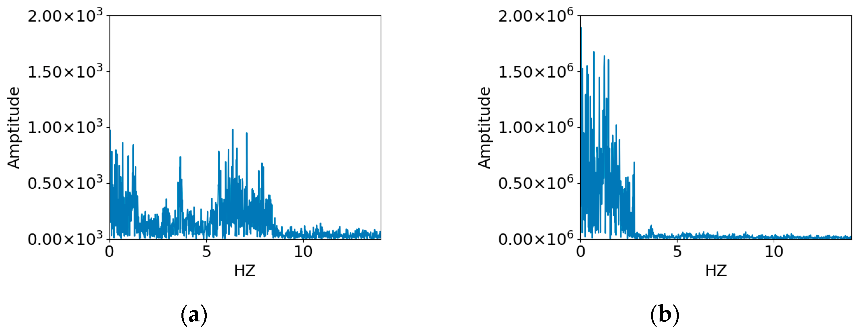
According to the power spectrum in the frequency domain (see Figure 2), the unit of the abscissa is HZ, and the ordinate is the amplitude. The acoustic signal energy of leakage in the valve is mainly concentrated within 1.5 Hz, while the acoustic signal energy distribution is relatively high when the valve is a normal width, distributed in the range of 0 to 8 Hz in Figure 2a. Therefore, valve leakage and normal state can be completely distinguished from the distribution of signal energy in the frequency domain. In addition, since the amplitude of the ordinate in Figure 2a is much smaller than that in Figure 2b, and we want to observe the difference in the energy distribution of the acoustic signal of the valve in two different states, that is, the distribution of the abscissa, we adjusted the appropriate ordinate. The range of the ordinate in Figure 2a is [0, 2.0 × 10³], and the range of the ordinate in Figure 2b is [0, 2.0 × 10⁶].

Figure 2.
AE signal spectrum in valve well−sealed normal conditions and leakage: (a) normal state and (b) leaked state.
2.3. Fault Diagnosis Method
In order to obtain features of data, PCA deposes the data matrix into a principal component subspace and a residual subspace. Among these, the principal component subspace reflects the change of standard data, and the residual subspace represents the noise of abnormal data. In other words, by projecting data into a smaller space, we reduce the dimensionality of our feature space. Consider an np data matrix , consisting of m variables and n samples; the Y is decomposed into the following form:
is the score matrix (, k is the number of principal components), is the score vectors, is the loading vectors, and is the residual matrix. The key statistics monitored by PCA are given by Hoteling’s T2:
Hoteling’s T2 statistic is a measure of the major variation in the variables and detects the fault if the variation in the latent variables is greater than it in the normal condition. The statistic, Q, is defined by:
The Q statistic, also named SPE, is the squared prediction error. It is a measure of the goodness of the fit of the new sample to the model. Since the statistic conforms to the F-distribution with a certain degree of confidence (usually 99%), the statistical is:
In the formula, is an F-distribution with degrees of freedom and the chosen level of significance , , α. The 100(1 − α)% control upper limit of Q is:
where is the sum of 1, 2, and 3 powers of the residual eigenvalues:
is the intermediate result variable,
To monitor multi-source data in production operation, two statistical indicators, and , can be used. A visual interpretation can better illustrate how PCA works, as shown in Figure 3.
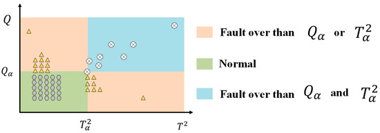
Figure 3.
A geometric interpretation for fault detection using two statistics.
If some sudden abnormal deviations occur on the variables, such as a mismatch between the actual variable and base variable, the T2 statistic is able to detect such violations. On the other hand, a change from the new data of the variables might violate the Q threshold. In other words, for fault detection, regions in Figure 3 with data points in the red area indicate abnormal events. In order to detect faults using T2 or SPE, the T2-contribution and Q-contribution plot represents the importance of each variable. The Q-contribution plot is defined as:
where is the contribution of each variable to the statistic SPE, , and is the i-th column of the identity matrix . The T2-contribution plot is defined as:
where , is the i-th column of the identity matrix , and represents the norm in phase space.
When the T2 or SPE exceeds the threshold, the contribution of the individual variables to the statistics can be identified, and the variable with the largest contribution is considered to be the potential fault source, which will be the input of the following fault prediction model.
2.4. Fault Prediction Models Using Deep Learning Method
In this section, an Informer model used for fault prediction, without ignoring relevant features across all time steps, is designed. Input at time t, and the output is the predicted value . When processing a sequence with a large time span and multiple inputs, the encoding and decoding structure is used to enhance the connection of the time sequence context for prediction.
The encoder inputs xt to hidden , and decodes from Ht to output . The full scheme of the deep learning fault clustering model is shown in Figure 4.
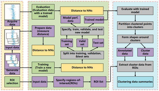
Figure 4.
Deep learning fault clustering scheme.
2.4.1. Efficient Self-Attention Mechanism
The self-attention mechanism uses queries, keys, and values to perform attention calculations. The specific calculation method is as follows:
where , , , d is the input dimension. The attention of the i-th query is defined as the probabilistic form:
To adaptively extract the driving sequence with attention weight:
The hidden status at the time instant of i can be updated to:
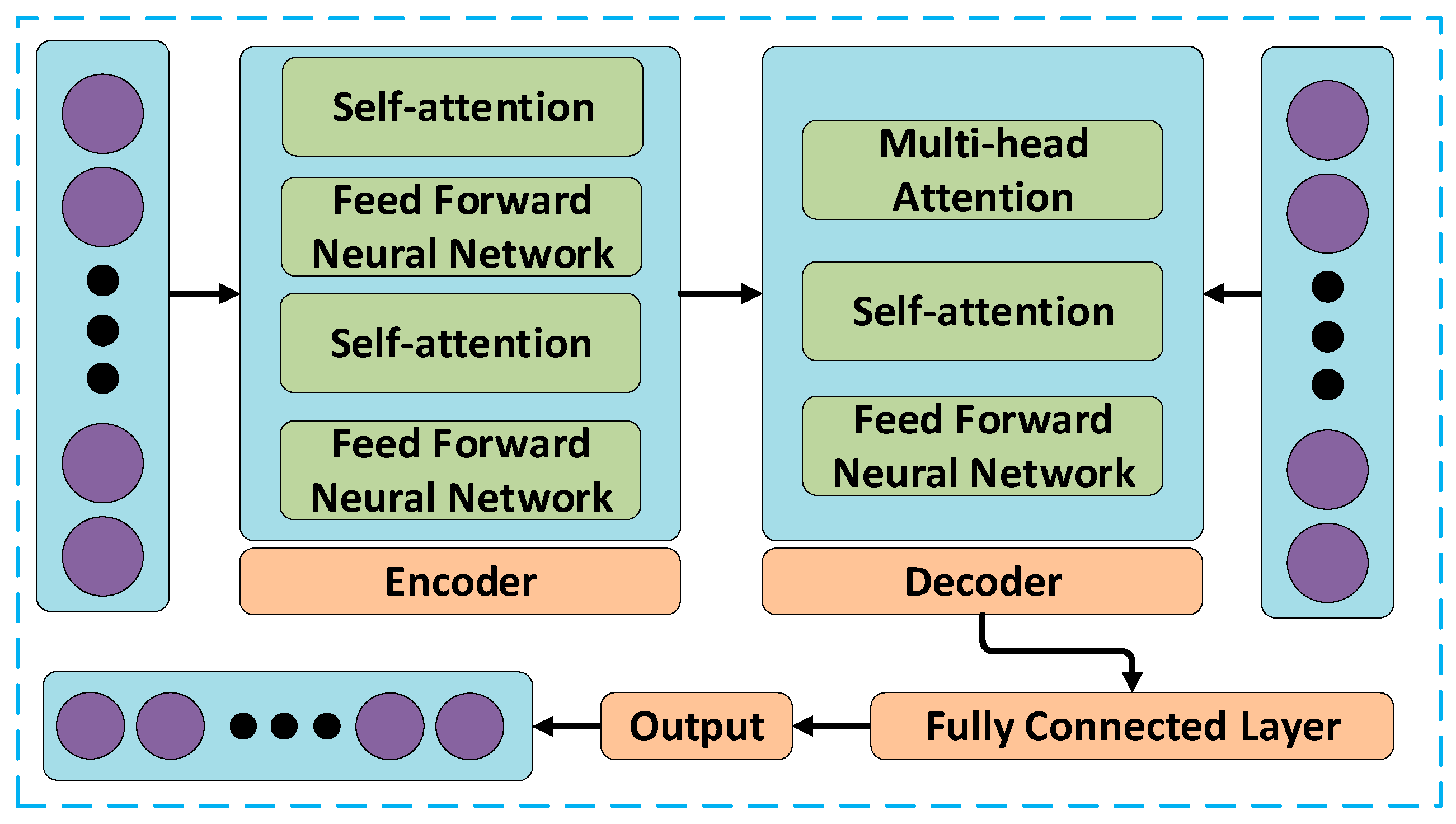
is a function of LSTM units, calculated according to Equations (3)–(7). is replaced with the newly calculated . Using the input attention mechanism, the encoder can selectively focus on certain driving sequences rather than treat all input driving series equally. The structure of the self-attention mechanism is shown in Figure 5.

Figure 5.
The architecture of encoder and decoder.
2.4.2. Decoder with Temporal Attention
In order to predict the output , another recurrent neural network based on LSTM is used to decode the encoded input information. The longer the input sequence, the worse the performance of the encoder and decoder. Therefore, a temporal attention mechanism is used in the decoder to adaptively select the relevant encoder hidden state across all time steps. Specifically, this is based on the previous hidden state of the decoder and the of the LSTM unit to calculate the attention weight of each encoder hidden state at time i.
where is a concatenation of the previous hidden state of the LSTM unit and the unit state. and are the parameters used for learning. Similarly, the offset term is also omitted here. The attention weight represents the importance of the i-th hidden state for prediction. Since each encoder hidden state is mapped to the temporal component of the input, the attention mechanism calculates the context vector as all encoder hidden states :
The context vector ci will be updated at each time step. Afterwards, the context vector is combined with the given target series :
where is a concatenation of the decoder input and the vector . The parameters and map the concatenation to the size of the decoder input. The newly calculated can be used to update the hidden state of the decoder at time i:
The non-linear function is selected as the unit. This function is widely used in long-term dependencies. can be updated as:
Informer uses an encoder to receive a large number of long sequences of input. In the encoder, ProbSparse is used to replace attention. We replaced the standard self-attention with the proposed ProbSparse. The attention is drawn to reduce the features extracted as the number of network layers increases to avoid the explosion of the network scale. The decoder receives a long sequence of inputs, calculates the attention of weighted features, and outputs a predicted value.
3. Experiments
3.1. Experiment Setup
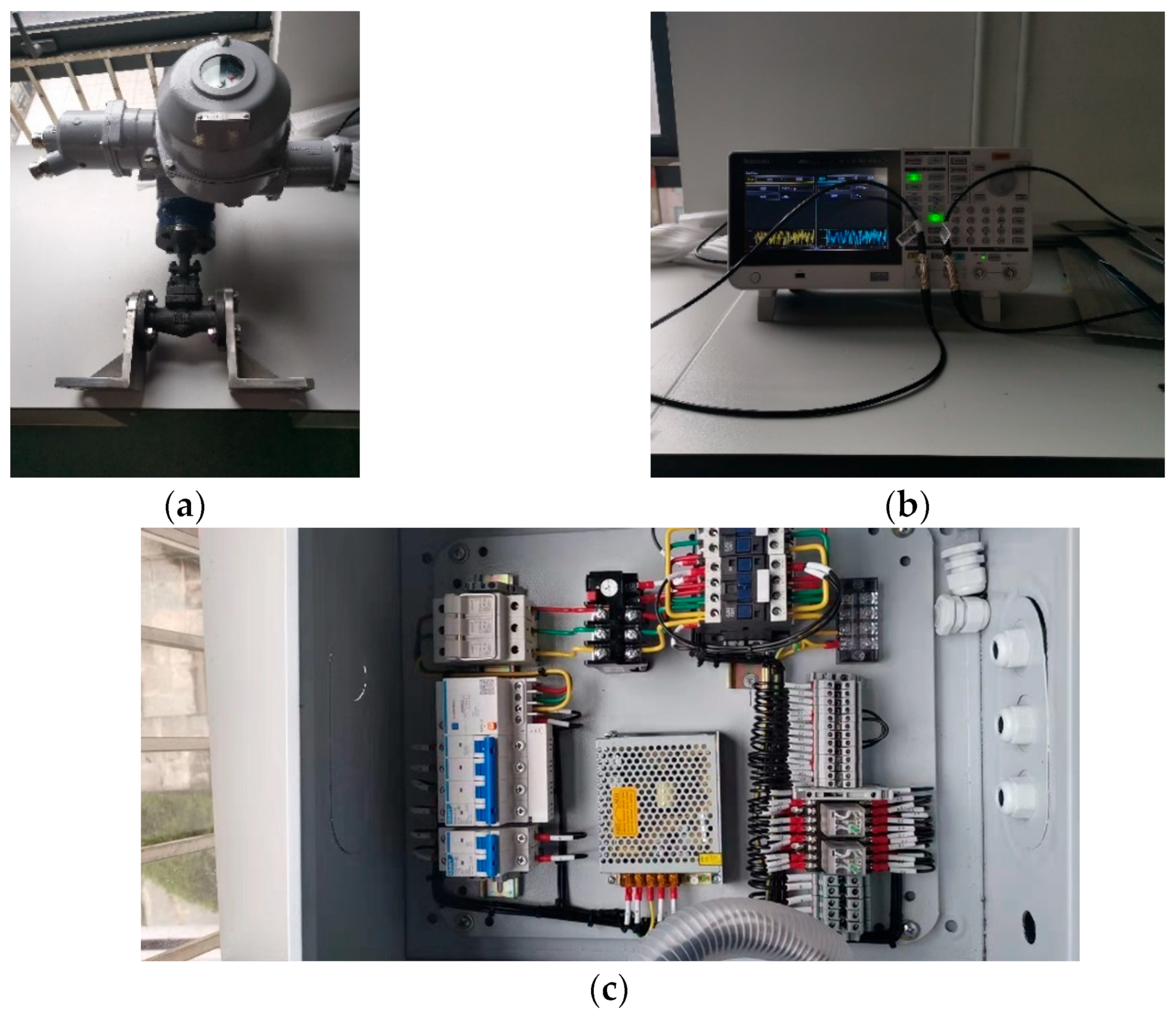
In order to verify the validity and advancement of the algorithm, a group of nuclear power valve detection devices are used to collect acoustic signals. We used four sensors to acquire acoustic signals simultaneously, so each group of acquired acoustic signals had a four-dimensional signal. Thus, each group of collected acoustic signals had four-dimensions. The acquisition of data was done by the oscilloscope. First, the sensor was connected to the valve, and the output was connected to the oscilloscope. After the circuit of the valve was opened, the acoustic signal collected by the sensor was converted into an electrical signal by the analog-to-digital converter (ADC) of the oscilloscope and displayed on the screen. The acquired data was displayed in a scrolling manner, starting on the right side of the display and continuing to the left side (while acquisition was in progress). In addition, the oscilloscope has mixed-signal acquisition memory, so all acoustic data would be stored in memory while the acquisition was in progress. As shown in Figure 6, Figure 6a is a nuclear power valve, Figure 6b is a signal generator, which can input and output acoustic signals, and Figure 6c is the control circuit of the nuclear power valve, which can control the start and stop of the valve.

Figure 6.
Nuclear power valve testing device: (a) nuclear power valve, (b) signal generator, and (c) control circuit of the nuclear power valve.
3.2. Data Preprocessing
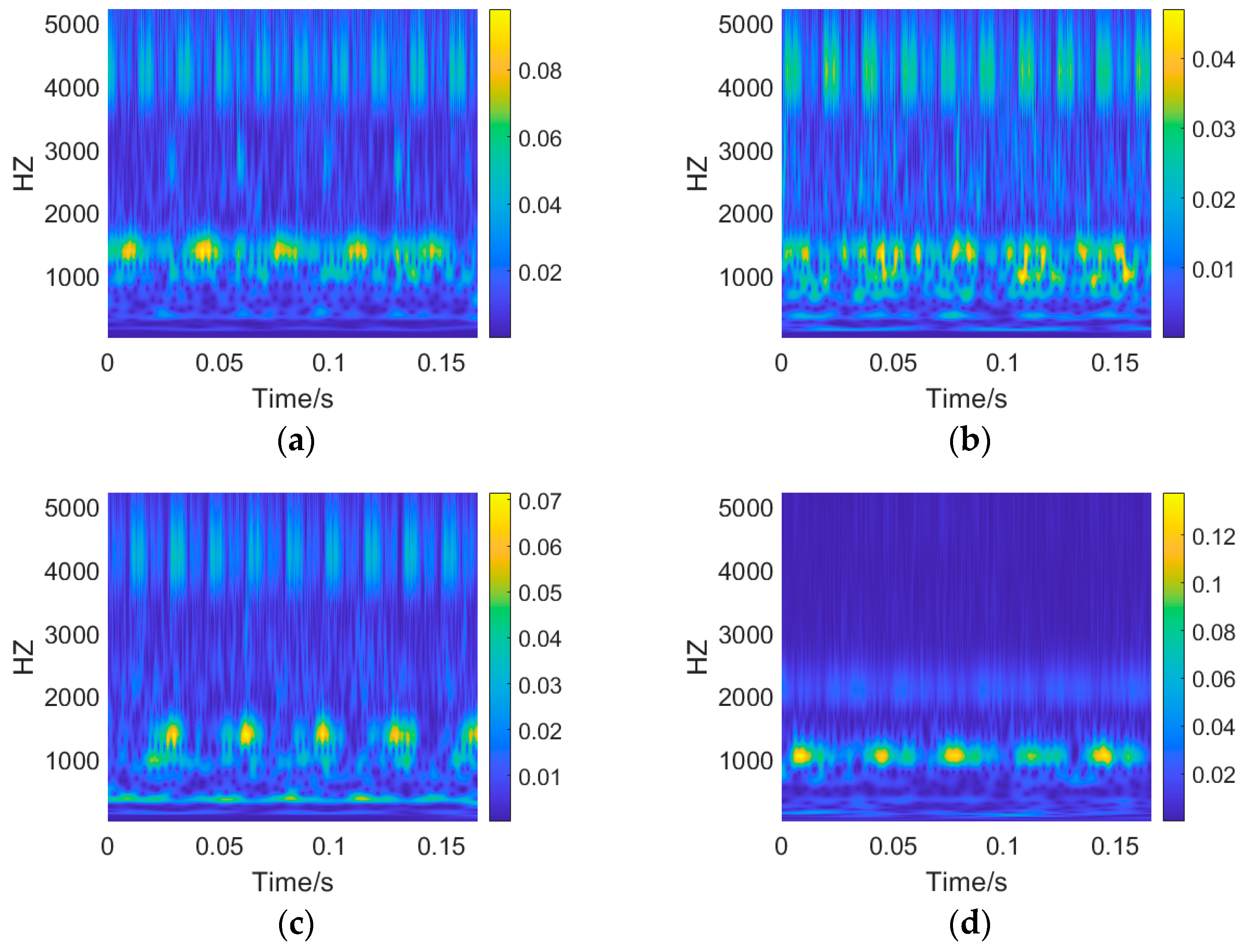
For long-term sequences of acoustic data containing many noisy signals, training with raw data is feasible but direct training is usually inefficient and, thus, requires feature extraction. Fourier transform and wavelet transform are common means of signal processing, but specific problems need to be analyzed in detail. If it is a stationary periodic signal, the Fourier transform is better, and if it is a non-stationary aperiodic signal, the wavelet is better. In addition, using wavelet transform to extract features and convert them into frequency domain images for subsequent fault classification can improve the accuracy of fault classification. Therefore, in this paper, the wavelet transform was chosen. Figure 7a–c are wavelet transform time–frequency diagrams of different types of fault signals, respectively, and Figure 7d is the wavelet transform time-frequency diagram of normal signals. After that, some unknown fault signals were input into the classifier. Since there are three types of faults, the classifier divides these input fault signals into three categories, A, B, and C, through clustering, which correspond to the Figure 7a–c three fault categories in Figure 7. Since there are three fault categories, we cluster the three different faults into three categories A, B, and C, corresponding to the three categories A, B, and C in Figure 8, respectively.
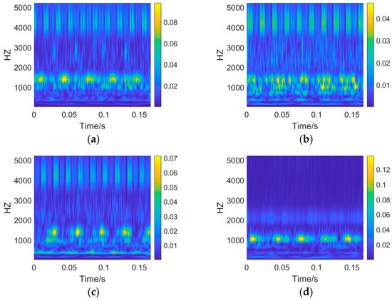
Figure 7.
Wavelet transform time–frequency diagram of fault and normal state time series for: (a) valve body leakage fault, (b) sealing surface leakage fault, (c) electric device fault and (d) normal signals.
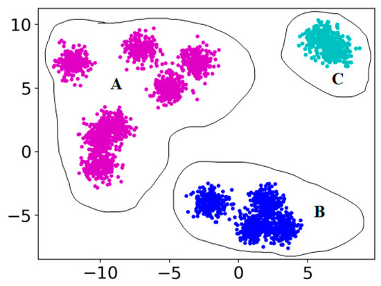
Figure 8.
Fault feature visualization.
3.3. Fault Detection Results for Electric Valves
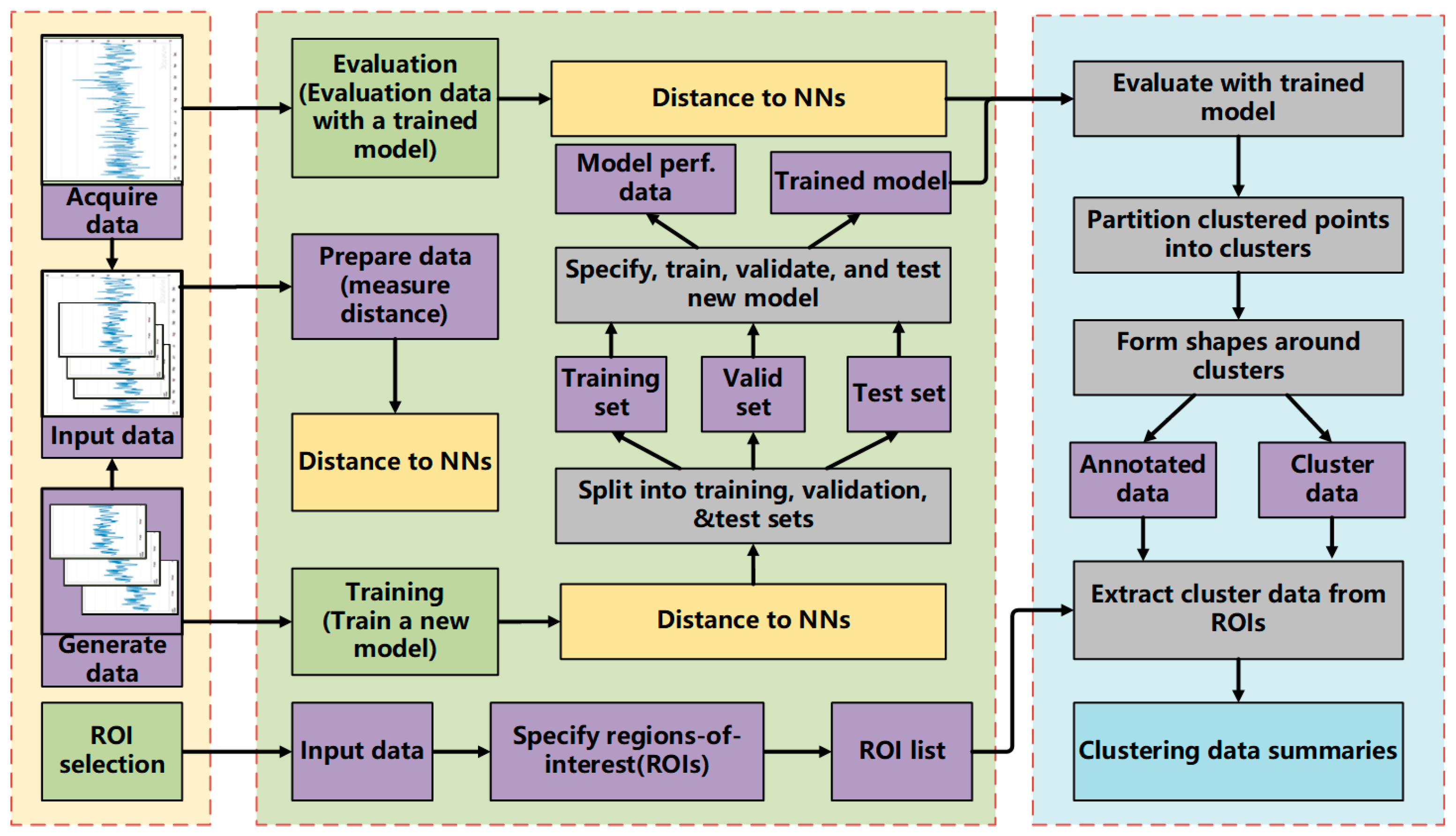
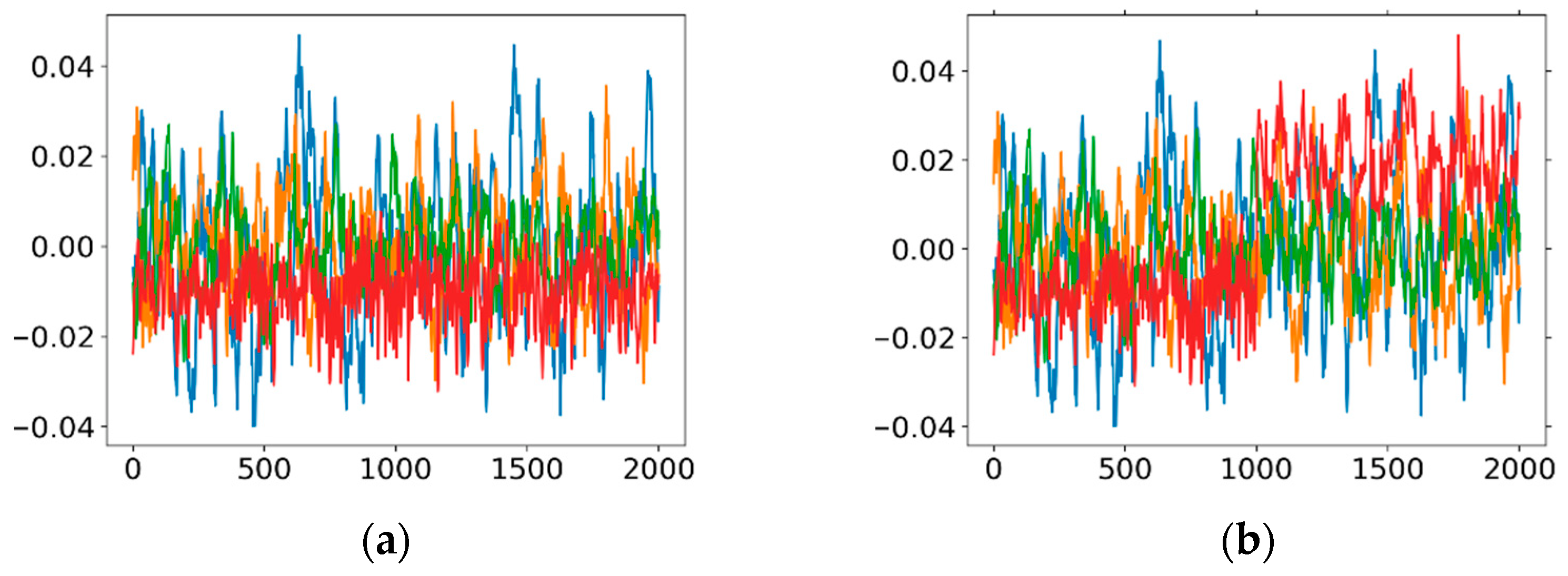
Since the valve acoustic signal of each fault state was collected simultaneously by four sensors during the experiment, each group of acoustic signals had four dimensions. For different kinds of acoustic signals, a set of 4D acoustic wave data, were selected as the training data for training the PCA model, and another set of 4D acoustic wave data were selected as test data to test the training model. For multi-dimensional time-series signals, it is difficult for us to distinguish small differences through human eyes. PCA can analyze the main components in the training data and reveal its main features. By computing the thresholds of the T2 and SPE statistics of the training data, if other classes of test data are fed into PCA, the thresholds will be exceeded and failure detection will succeed. Therefore, in this paper, we applied PCA for fault detection, and the train data and test data are shown in Figure 9a,b.

Figure 9.
Fault detection results: (a) training data set and (b) testing data.
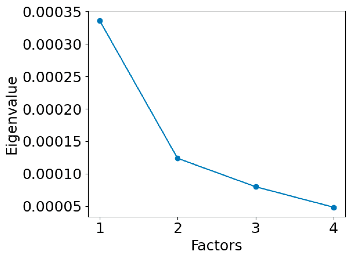
Figure 10 shows the results of sorting the eigenvalues and outputting them in descending order during the PCA modelling. It can be seen from the figure that the gap between the first three eigenvalues and the last eigenvalue is too large. Therefore, it can be considered that the last eigenvalue is less important, and, thus, the first three eigenvalues are taken as the principal components. This process can be understood as dimensionality reduction, which can compress data while minimizing information loss. For fault detection, it can compress data and extract the features at the same time.

Figure 10.
Sorted eigenvalues with descending order.
We selected three principal components, namely three eigenvalues. From the perspective of vector space, because the eigenvectors corresponding to different eigenvalues are linearly independent, each eigenvector is regarded as a coordinate axis, and the eigenvalue is the coordinate value of the corresponding coordinate axis (i.e., the eigenvector). In simple terms, the original matrix is represented by eigenvalues (coordinates) and eigenvectors (coordinate axes). Since we cannot plot the four-dimensional space, to better understand the relationship between the eigenvectors, Figure 11 shows a heatmap formed by the matrix of eigenvectors corresponding to the selected principal components.
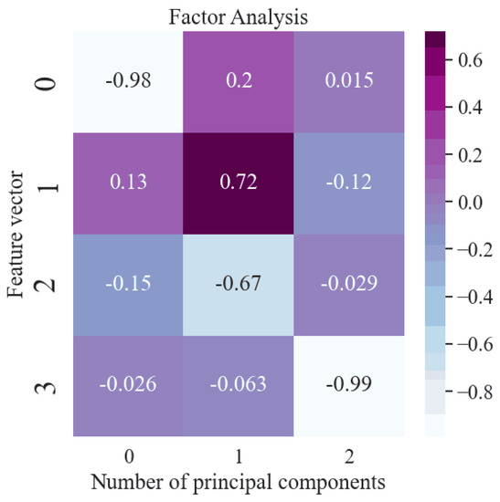
Figure 11.
Eigenvector matrix corresponding to principal components.
The thresholds for the T2 and SPE statistics can be obtained from the training data by PCA, and T2 and SPE statistics can be obtained from test data by PCA. The T2 statistic reflects the degree to which each principal component deviates from the model, in terms of variation trend and amplitude. It is a measure of the internalization of the model, and it can be used to monitor multiple principal components at the same time. The SPE statistic describes the degree of deviation of the measured value of the input variable from the principal component model, which is a measure of the external changes of the model. Figure 12 shows the results of PCA fault detection, where the red straight line represents the thresholds for the T2 and SPE statistics. If the T2 or SPE statistics exceed the thresholds, it means a fault has occurred and the red dotted rectangular box area is marked as the fault state.
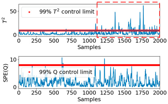
Figure 12.
The results of principal component analysis.
3.4. Fault Prediction Results for Electric Valves
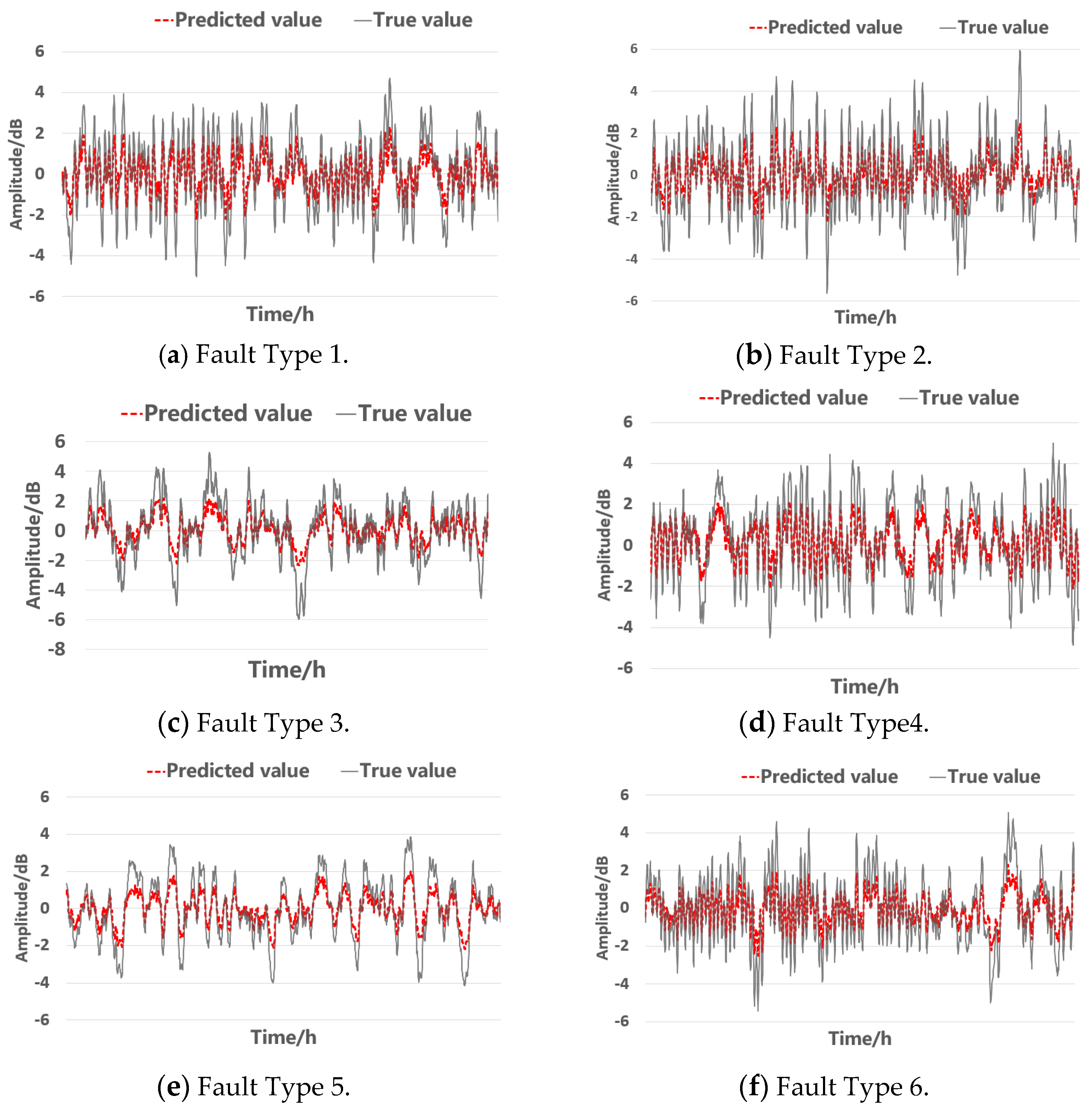
In Figure 13, in order to verify the validity of the Informer model for fault prediction, six different fault categories were used for the experiments, and the results of the actual and predicted values are shown as well. The red dotted line represents the predicted value, and the black solid line represents the true value. In addition, the performance evaluation indicators of each group of experimental results have been listed in Table 1. It can be seen from Figure 13 that the change trend of the predicted value is consistent with the actual value, and the change trend of the time-series signal can be effectively predicted. However, from the evaluation index between the predicted value and the actual value in Table 1, it can be seen that there are still some differences between the predicted value and the actual value. This is because we used acoustic wave data, and the sampling noise was relatively obvious. The literature [28] also mentioned that, on different data sets, the prediction effect of the Informer model has certain differences. In the future, we will start by changing the sampling rate, reducing noise, and adjusting the parameters of the prediction model to increase the success rate of fault prediction.

Figure 13.
Long time–series fault prediction.

Table 1.
Fault prediction result evaluation index.
4. Conclusions
This paper proposes a PCA–Informer model, aiming at the fault detection and prediction of nuclear valves. The first stage selects the features that need attention, and the second stage uses an Informer attention mechanism to decode the hidden state for the prediction. Since it not only uses an input attention mechanism to relevant driving series but also employs an attention mechanism to select relevant hidden features across all time steps, the experimental results demonstrate that the PCA–Informer model can successfully achieve an accurate result in fault detection and prediction. Therefore, a safe online monitoring of key elements in nuclear stations, such as electrical valves, can be realized on a regular basis, and maintenance time and cost can be reduced. Meanwhile, fault diagnoses and predictions can be carried out with high accuracy to prevent potential hazards to operators and a waste of nuclear equipment.
Author Contributions
Conceptualization, Z.A., Y.G., B.S., W.C., Y.L. and Z.Y.; data curation, Z.A., Y.G., H.C. and W.C.; formal analysis, L.C., Y.G., B.S. and H.C.; funding acquisition, J.L., H.C., W.C., Y.L. and Z.Y.; investigation, W.F., B.S., J.L., Y.L. and Z.Y.; methodology, B.S.; project administration, M.R., W.F. and Z.Y.; resources, M.R., W.F. and J.L.; software, Z.A. and B.S.; supervision, Y.G., M.R., W.F., W.C. and Z.Y.; validation, M.R. and H.C.; visualization, Z.A.; writing—original draft, Z.A., L.C., Y.G. and W.F.; writing—review and editing, Z.A., L.C., Y.G., M.R., J.L. and Z.Y. All authors have read and agreed to the published version of the manuscript.
Funding
This research was funded by State Key Laboratory of Nuclear Power Safety Monitoring Technology and Equipment [K-A2020.407], National Science Foundation of China [52077213, 62073232 and 62003332], Joint Research Fund between the National Natural Science Foundation of China and Shenzhen [U1813222, U20A20283], The Natural Science Foundation of Shanxi Province, China [202103021231], and Guangdong special branch plans young talent with scientific and technological innovation [2019TQ05Z654].
Institutional Review Board Statement
Not applicable.
Informed Consent Statement
Not applicable.
Data Availability Statement
Not applicable.
Acknowledgments
The authors would like to thank State Key Laboratory of Nuclear Power Safety Monitoring Technology and Equipment for their support of this research. The authors would like to thank the all the reviewers for their constructive comments.
Conflicts of Interest
The authors declare no conflict of interest.
References
- Gao, Z.; Cecati, C.; Ding, S.X. A Survey of Fault Diagnosis and Fault-Tolerant Techniques—Part I: Fault Diagnosis with Model-Based and Signal-Based Approaches. IEEE Trans. Ind. Electron. 2015, 62, 3757–3767. [Google Scholar] [CrossRef] [Green Version]
- Lei, Y.; Yang, B.; Jiang, X.; Jia, F.; Li, N.; Nandi, A.K. Applications of machine learning to machine fault diagnosis: A review and roadmap. Mech. Syst. Signal Process. 2020, 138, 106587. [Google Scholar] [CrossRef]
- Liu, R.; Yang, B.; Zio, E.; Chen, X. Artificial intelligence for fault diagnosis of rotating machinery: A review. Mech. Syst. Signal Process. 2018, 108, 33–47. [Google Scholar] [CrossRef]
- Jiao, J.; Zhao, M.; Lin, J.; Liang, K. A comprehensive review on convolutional neural network in machine fault diagnosis. Neurocomputing 2020, 417, 36–63. [Google Scholar] [CrossRef]
- Kordestani, M.; Zanj, A.; Orchard, M.E.; Saif, M. A modular fault diagnosis and prognosis method for hydro-control valve system based on redundancy in multi-sensor data information. IEEE Trans. Reliab. 2018, 68, 330–341. [Google Scholar] [CrossRef]
- Liu, C.; Wang, Y.; Pan, T.; Zheng, G. Fault diagnosis of electro-hydraulic servo valve using extreme learning machine. Int. Trans. Electr. Energy Syst. 2020, 30, e12419. [Google Scholar] [CrossRef]
- Yucesan, Y.A.; Dourado, A.; Viana, F. A survey of modeling for prognosis and health management of industrial equipment. Adv. Eng. Inform. 2021, 50, 101404. [Google Scholar] [CrossRef]
- Xu, B.; Shen, J.; Liu, S.; Su, Q.; Zhang, J. Research and Development of Electro-hydraulic Control Valves Oriented to Industry 4.0: A Review. Chin. J. Mech. Eng. 2020, 33, 29. [Google Scholar] [CrossRef] [Green Version]
- Djeziri, M.; Djedidi, O.; Benmoussa, S.; Bendahan, M.; Seguin, J.L. Failure Prognosis Based on Relevant Measurements Identification and Data-Driven Trend-Modeling: Application to a Fuel Cell System. Processes 2021, 9, 328. [Google Scholar] [CrossRef]
- Li, X.; Ren, P.; Zhang, Z.; Jia, X.; Peng, X. A p−V Diagram Based Fault Identification for Compressor Valve by Means of Linear Discrimination Analysis. Machines 2022, 10, 53. [Google Scholar] [CrossRef]
- Chen, H.; Xiong, Y.; Li, S.; Song, Z.; Hu, Z.; Liu, F. Multi-Sensor Data Driven with PARAFAC-IPSO-PNN for Identification of Mechanical Nonstationary Multi-Fault Mode. Machines 2022, 10, 155. [Google Scholar] [CrossRef]
- Shi, S.; Li, G.; Chen, H.; Hu, Y.; Wang, X.; Guo, Y.; Sun, S. An efficient VRF system fault diagnosis strategy for refrigerant charge amount based on PCA and dual neural network model. Appl. Therm. Eng. 2018, 129, 1252–1262. [Google Scholar] [CrossRef]
- Liu, Z.; Liu, J.; Huang, Y.; Li, T.; Nie, C.; Xia, Y.; Zhan, L.; Tang, Z.; Zhang, L. Fault Critical Point Prediction Method of Nuclear Gate Valve with Small Samples Based on Characteristic Analysis of Operation. Materials 2022, 15, 757. [Google Scholar] [CrossRef]
- Xu, R.; Peng, M.; Wang, H. Study on the Condition Monitoring Technology of Electric Valve Based on Principal Component Analysis. In Proceedings of the International Congress and Workshop on Industrial AI 2021, Luleå, Sweden, 5–7 October 2021; Springer: Cham, Switzerland, 2021; pp. 141–151. [Google Scholar]
- Han, X.; Jiang, J.; Xu, A.; Huang, X.; Pei, C.; Sun, Y. Fault Detection of Pneumatic Control Valves Based on Canonical Variate Analysis. IEEE Sens. J. 2021, 21, 13603–13615. [Google Scholar] [CrossRef]
- Lv, Q.; Yu, X.; Ma, H.; Ye, J.; Wu, W.; Wang, X. Applications of Machine Learning to Reciprocating Compressor Fault Diagnosis: A Review. Processes 2021, 9, 909. [Google Scholar] [CrossRef]
- Zhang, Z.; Li, B.; Zhang, W.; Lu, R.; Wada, S.; Zhang, Y. Real-time penetration state monitoring using convolutional neural network for laser welding of tailor rolled blanks. J. Manuf. Syst. 2020, 54, 348–360. [Google Scholar] [CrossRef]
- Kumar, P.; Hati, A.S. Review on machine learning algorithm based fault detection in induction motors. Arch. Comput. Methods Eng. 2021, 28, 1929–1940. [Google Scholar] [CrossRef]
- Jan, S.U.; Lee, Y.D.; Koo, I.S. A distributed sensor-fault detection and diagnosis framework using machine learning. Inf. Sci. 2021, 547, 777–796. [Google Scholar] [CrossRef]
- Bode, G.; Thul, S.; Baranski, M.; Müller, D. Real-world application of machine-learning-based fault detection trained with experimental data. Energy 2020, 198, 117323. [Google Scholar] [CrossRef]
- Yuan, H.; Wu, N.; Chen, X.; Wang, Y. Fault Diagnosis of Rolling Bearing Based on Shift Invariant Sparse Feature and Optimized Support Vector Machine. Machines 2021, 9, 98. [Google Scholar] [CrossRef]
- Ali, Y.H. Artificial intelligence application in machine condition monitoring and fault diagnosis. Artif. Intell. Emerg. Trends Appl. 2018, 275, 464. [Google Scholar] [CrossRef]
- Nath, A.G.; Udmale, S.S.; Singh, S.K. Role of artificial intelligence in rotor fault diagnosis: A comprehensive review. Artif. Intell. Rev. 2021, 54, 2609–2668. [Google Scholar] [CrossRef]
- Sony, S.; LaVenture, S.; Sadhu, A. A literature review of next-generation smart sensing technology in structural health monitoring. Struct. Control Health Monit. 2019, 26, e2321. [Google Scholar] [CrossRef]
- Ye, X.W.; Jin, T.; Yun, C.B. A review on deep learning-based structural health monitoring of civil infrastructures. Smart Struct. Syst. 2019, 24, 567–585. [Google Scholar]
- Han, K.; Xiao, A.; Wu, E.; Guo, J.; Xu, C.; Wang, Y. Transformer in transformer. Adv. Neural Inf. Process. Syst. 2021, 34, 1–12. [Google Scholar]
- Wu, N.; Green, B.; Ben, X.; O’Banion, S. Deep transformer models for time series forecasting: The influenza prevalence case. arXiv 2020, arXiv:2001.08317. [Google Scholar]
- Zhou, H.; Zhang, S.; Peng, J.; Zhang, S.; Li, J.; Xiong, H.; Zhang, W. Informer: Beyond efficient transformer for long sequence time-series forecasting. In Proceedings of the AAAI virtually, New York, NY, USA, 2–9 February 2021. [Google Scholar]
- Kitaev, N.; Kaiser, Ł.; Levskaya, A. Reformer: The efficient transformer. arXiv 2020, arXiv:2001.04451. [Google Scholar]
- Correia, G.M.; Niculae, V.; Martins, A.F. Adaptively sparse transformers. arXiv 2019, arXiv:1909.00015. [Google Scholar]
- Beltagy, I.; Peters, M.E.; Cohan, A. Longformer: The long-document transformer. arXiv 2020, arXiv:2004.05150. [Google Scholar]
- Pandey, U.K.; Pal, S. Data Mining: A prediction of performer or underperformer using classification. arXiv 2011, arXiv:1104.4163. [Google Scholar]
- Child, R.; Gray, S.; Radford, A.; Sutskever, I. Generating long sequences with sparse transformers. arXiv 2019, arXiv:1904.10509. [Google Scholar]
- Dai, Z.; Yang, Z.; Yang, Y.; Carbonell, J.; Le, Q.; Salakhutdinov, R. Transformer-xl: Attentive language models beyond a fixed-length context. arXiv 2019, arXiv:1901.02860. [Google Scholar]
- Lee, E.R.; Cho, J.; Yu, K. A systematic review on model selection in high-dimensional regression. J. Korean Stat. Soc. 2018, 48, 1–12. [Google Scholar] [CrossRef]
- Guo, Y.; Li, K.; Laverty, D.; Xue, Y. Synchrophasor-Based Islanding Detection for Distributed Generation Systems Using Systematic Principal Component Analysis Approaches. IEEE Trans. Power Deliv. 2015, 30, 2544–2552. [Google Scholar] [CrossRef] [Green Version]
- Zhu, J.; Yang, Z.; Mourshed, M.; Guo, Y.; Zhou, Y.; Chang, Y.; Wei, Y.; Feng, S. Electric Vehicle Charging Load Forecasting: A Comparative Study of Deep Learning Approaches. Energies 2019, 12, 2692. [Google Scholar] [CrossRef] [Green Version]
- Qian, H.; Sun, B.; Guo, Y.; Yang, Z.; Ling, J.; Feng, W. A parallel deep learning algorithm with applications in process monitoring and fault prediction. Comput. Electr. Eng. 2022, 99, 107724. [Google Scholar] [CrossRef]
Publisher’s Note: MDPI stays neutral with regard to jurisdictional claims in published maps and institutional affiliations. |
© 2022 by the authors. Licensee MDPI, Basel, Switzerland. This article is an open access article distributed under the terms and conditions of the Creative Commons Attribution (CC BY) license (https://creativecommons.org/licenses/by/4.0/).


