Abstract
This article deals with the development of a simple model to evaluate the first natural frequencies of over-constrained parallel kinematic machines (PKMs). The simplest elasto-dynamic models are based on multi-body approaches. However, these approaches require an expression of the Jacobian matrices that may be difficult to obtain for complex PKMs. Therefore, this paper focuses on the determination of the global mass and stiffness matrices of an over-constrained PKM in stationary configurations without the use of Jacobian matrices. The PKM legs are modeled by beams. Because the legs are connected to a moving platform and the mechanism is over-constrained, constraint equations between the parameters that model the deformation of each leg are determined according to screw theory. The first natural frequencies and associated modes can then be determined. It should be noted that the proposed method can be easily used at the conceptual design stage of PKMs. The Tripteor X7 machine is used as an illustrative example and is characterized experimentally.
1. Introduction
Parallel Kinematic Robots are used in many fields such as medicinal, aerospace, rehabilitation, and astronomy [1]. In industry, parallel kinematic robots are mainly used for pick-and-place operations [2]. However, a few Parallel Kinematic Machine Tools (PKMs) are used in the automotive or aeronautical industries for High-Speed Machining (HSM) operations [3]. Their dynamic performances, in terms of acceleration, are better for an equivalent motorization than Serial Kinematic Machine Tools (SKMs) due their closed-loop architecture [4]. However, the design of these closed-loop architectures imposes to control leg size that reduces mobile masses and leads to a loss of stiffness compared to SKM [5,6].
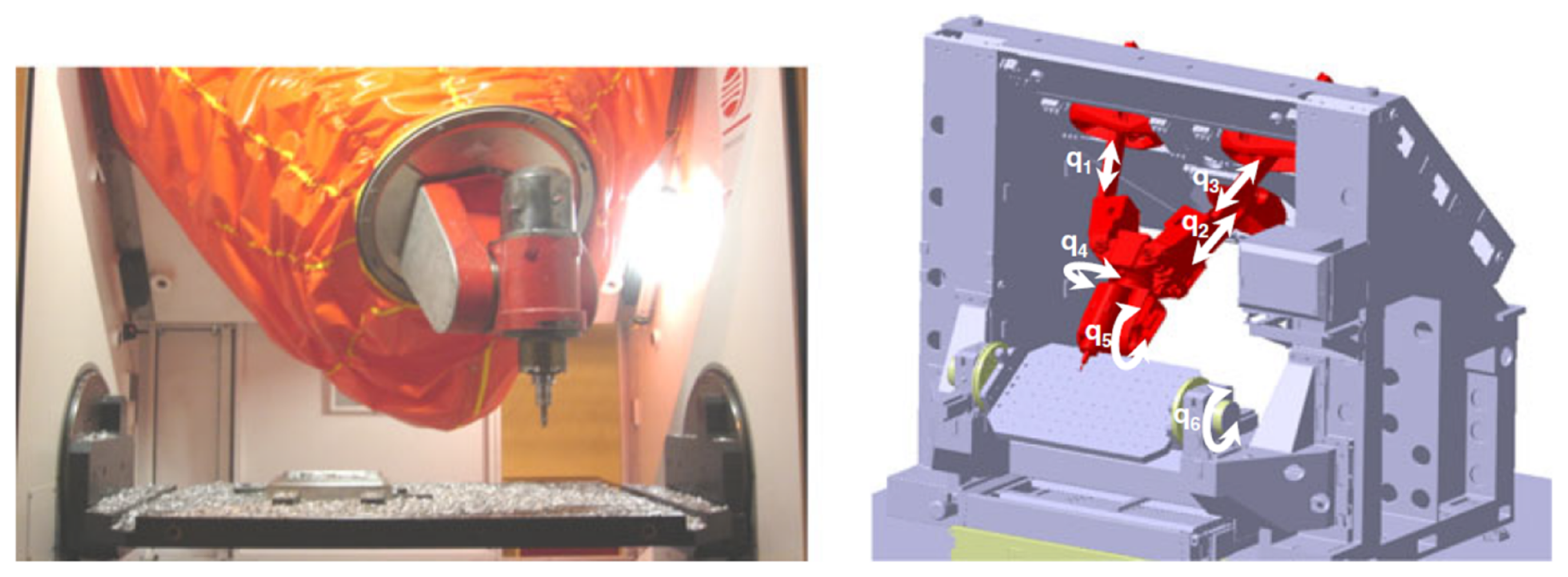
One way to improve PKM stiffness behavior is to use an over-constrained architecture. To this aim, an over-constrained PKM, named Exechon, was designed by Neumann [7], and the PCI-SCEMM company chose to integrate an Exechon robot into the design of Tripteor X7 machine tool (Figure 1). An over-constrained system is considered to be a hyperstatic system which is defined by the IFToMM terminology as a system in which the distribution of internal forces depends on the material properties of the members of the system [8]. Thus, an over-constrained PKM is defined as a PKM with common or redundant constraints that can be removed without changing the kinematic properties of the mechanism [9]. Thus, the study of an over-constrained mechanism behavior can be complex due to the generation of static indeterminacy and geometric constraints [10].
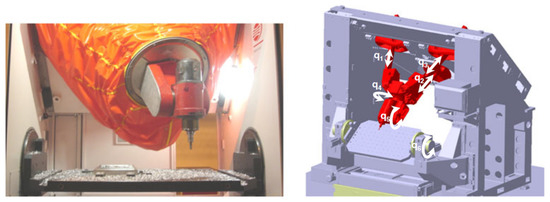
Figure 1.
Tripteor X7 Parallel Kinematic Machine Tools.
Previous work highlights the impact on part quality of PKM vibrations during machining [11]. Depending on the machined part position, marks appear on the machined surfaces. To minimize these vibrations, it is of prime importance to express a parameterized elasto-dynamic model for over-constrained PKMs. Such a model enables the prediction of static and vibration behavior during the conceptual design stage. Moreover, as PKM behavior is anisotropic and changes regarding the tool pose, the elasto-dynamic model of the PKM should be fast to compute to quickly obtain its stiffness, its first natural frequencies and associated modes throughout the manipulator workspace.
Two main methods are classically used in the literature to express the elasto-dynamic model of an over-constrained PKM:
- Finite Element Analysis (FEA): this method is the most accurate one, but it requires the exact definition of the mechanism components. It is usually used for validation purposes at the final design stage since it is time-consuming [12,13,14,15].
- Multi-body approaches: PKM legs can be modeled, for example, using beam theory and their joint behavior relies on Virtual Joint Method (VJM) [16,17]. In the literature, the simplest elasto-dynamic models are based on multi-body approaches. This method can only be applied for robot architectures whose hypotheses are valid. Other formulations are introduced to consider large deformations of flexible manipulators [18] or to decrease simulation time for complex mechanisms such as Matrix Structural Analysis (MSA) [19]. The decreasing of the time simulation is generally based on the development of a methodology to merge stiffness and mass matrices of all elements of the mechanism [19,20].
In this article, multi-body approach, a robust but simple approach to obtain a parameterized elasto-dynamic model, is preferred to the use of complex and time-consuming FEA. The prediction of vibration phenomena requires the determination of the first natural frequencies and their associated modes. In [16,17], this is performed by computing the global mass matrix and the global stiffness matrix. However, the computation of mass and stiffness matrices is complex in the case of over-constrained mechanisms such as Exechon PKM. Indeed, the complex coupling between displacement vector components due to over-constrained properties must be considered during the sub-systems matrix assembly stage. Thus, the application of this approach to over-constrained PKMs requires the determination of Jacobian matrices to characterize kinematic dependencies due to closed-loop over-constrained mechanisms [16,21] or the definition of a complex methodology to merge stiffness matrices of each PKM element [19]. Those Jacobian matrices describe the kinematic behavior of PKMs by derivation of the geometric model as in Germain’s [16] and Zhang’s [17] works. Geometric model or closed-loop constraints of complex PKM, such as Exechon robot, can sometimes not be computed in a systematic and straightforward way [16,22]. For example, the expression of the geometric model of an Exechon robot is based on a system of nonlinear equations that are not easy to establish [23]. Moreover, its solving requires a numerical optimization with the Newton-Raphson method.
This paper aims to introduce a reliable and simple method to compute global mass and stiffness matrices for over-constrained PKMs, under the assumption of small displacements and using screw theory. This methodology is relevant for high-stiffness architectures such as machine tools and industrial robots where flexibility generates only small displacements. These mathematical tools allow defining geometric dependencies of leg movements without the computation of Jacobian matrices [24]. Screw theory is used both:
- To express the kinematic behavior of each PKM leg using the theory of Timoshenko beams [25] and
- To determine the displacement constraints applied to each leg extremity due to over-constrained mechanism closed-loops [26].
There are different ways to parameterize the orientation of a rigid body such as quaternion [27]. The choice of screw theory ensures use of the same representation for the actuation and constraint wrenches applied to the moving platform by the actuators and the geometry of the mechanism.
This second point is the main contribution of our work and allows us to take into account stress due to over-constrained with geometric constraint equations extracted only from the screw theory application to the passive joints. With this method, the computation of global mass and stiffness matrices is easy to implement. It assumes only geometrical constraints between displacement vector components without the introduction of the Jacobian matrices. Global mass and stiffness matrices are then computed to estimate PKM Cartesian stiffness, the first natural frequencies and their associated modes. This work is relevant at the embodiment design stage of the robot when only a parameterized CAD modeling of the PKM under study is available. Indeed, at this stage, a fast computation time is required to assess the capability of the PKM in terms of vibration behavior and to determine the optimal architecture and dimensions of the robot under design. During the next design stages, when accurate simulation results are needed, FEA can be preferred although it is more computation intensive.
It should be noted that the revolute joints of the Tripteor legs are stiff; their stiffness is larger than N·m−1 [28]. Moreover, the stiffness of the spherical wrist of the Tripteor is even more important. As a consequence, and for the sake of clarity, only the deflection of Tripteor X7 PKM legs is considered in what remains. The joint deflection can be taken into account by adding local stiffness such as with the Virtual Joint Method [29].
The paper is organized as follows: Section 2 presents the Tripteor X7 PKM and its parametrization. Section 3 describes the proposed method to express the elasto-dynamic model of PKMs and to compute their natural frequencies. As an illustrative example, the stiffness matrix, the natural frequencies and associated modes of the Tripteor X7 PKM are computed in Section 4. Finally, conclusions and future work are drawn in Section 5.
2. Tripteor X7 PKM
Tripteor X7 PKM is manufactured by the PCI-SCEMM company in France. It is a hybrid PKM. Its architecture is a combination of a parallel mechanism and a serial wrist mounted in series. Such a hybrid manipulator ensures the decoupling of translational and rotational motion of the end-effector. Moreover, hybrid manipulators usually have a better dexterity than fully parallel manipulators as explained in [30].
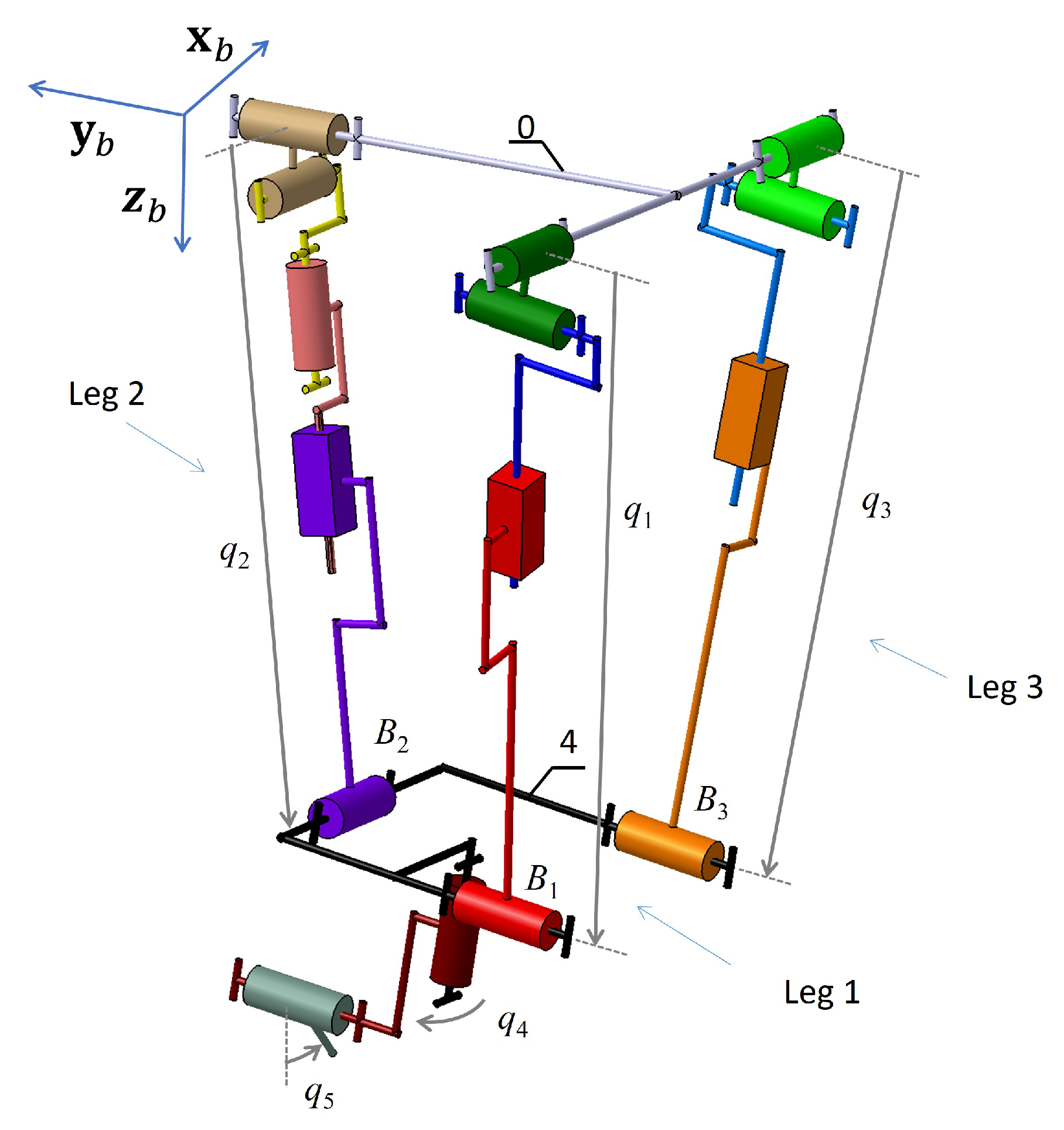
Tripteor X7 PKM is a six-axis PKM with the following actuated joint variables shown in Figure 2 and one-DoF rotary table represented in Figure 1. The revolute joint variable of this rotary table is denoted as . A parallel mechanism provides three Degrees of Freedom (DoFs) from the actuation of three ball screw systems (, and ) and a serial wrist with two DoFs from the actuation of two revolute joints with direct and belt drives ( and ). The elongations , and of Leg 1, Leg 2 and Leg 3 provide translational motions of the moving platform along axis , and axis with induced rotational motions about axis and axis . The serial wrist ensures rotational motions of the end-effector.
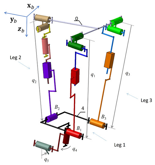
Figure 2.
Kinematic model of Tripteor X7 PKM.
The paper aims to introduce a new methodology to compute natural frequencies of over-constrained closed-loop mechanism in the case of PKM. Thus, only the vibration behavior of the parallel mechanism composed of Leg 1, Leg 2, Leg 3 and the mobile platform (4) is studied in this paper (Figure 2). If a study of the complete PKM should be carried, a simple assembly of global mass and stiffness matrices of the parallel mechanism and the serial wrist can then be carried out.
Each leg is connected to the mobile platform (4) by a revolute joint and to the fixed platform (0) by two revolute joints which form a universal joint (Figure 2). It is worth noting that Leg 2 has a supplementary revolute joint around its principal axis. Consequently, bending and traction-compression loads are prescribed to Leg 2 whereas Legs 1 and 3 are loaded in bending, traction-compression, and torsion [28]. The mobile platform is supposed to be rigid. Because stiffness and low frequencies are of primal importance in machining [11], an efficient and fast way to compute those frequencies is described in this paper. For this purpose, a local model of a PKM leg under bending, traction-compression, and torsion loads is introduced before the definition of constraint equations due to mechanism assembly.
3. Elasto-Dynamic Modeling of PKMs
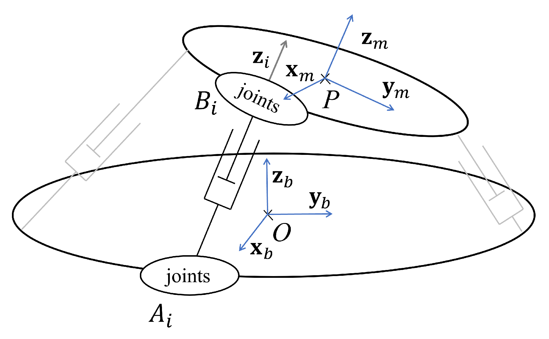
This section introduces the novel elasto-dynamic modeling approach and its application to PKMs. For the sake of pedagogy, we introduce our method for PKMs with telescopic legs such as the Tripteor X7 (Figure 3). and are the leg extremities. is attached to the PKM base and is fixed to the mobile platform. The coordinate system associated with the fixed base is denoted as and with the mobile platform as . is the unit vector along leg i direction.

Figure 3.
Definition of used parameters for PKM with telescopic legs.
This method can be applied to any PKMs whose legs can be modeled by beams.
3.1. Local Modeling of PKM Leg
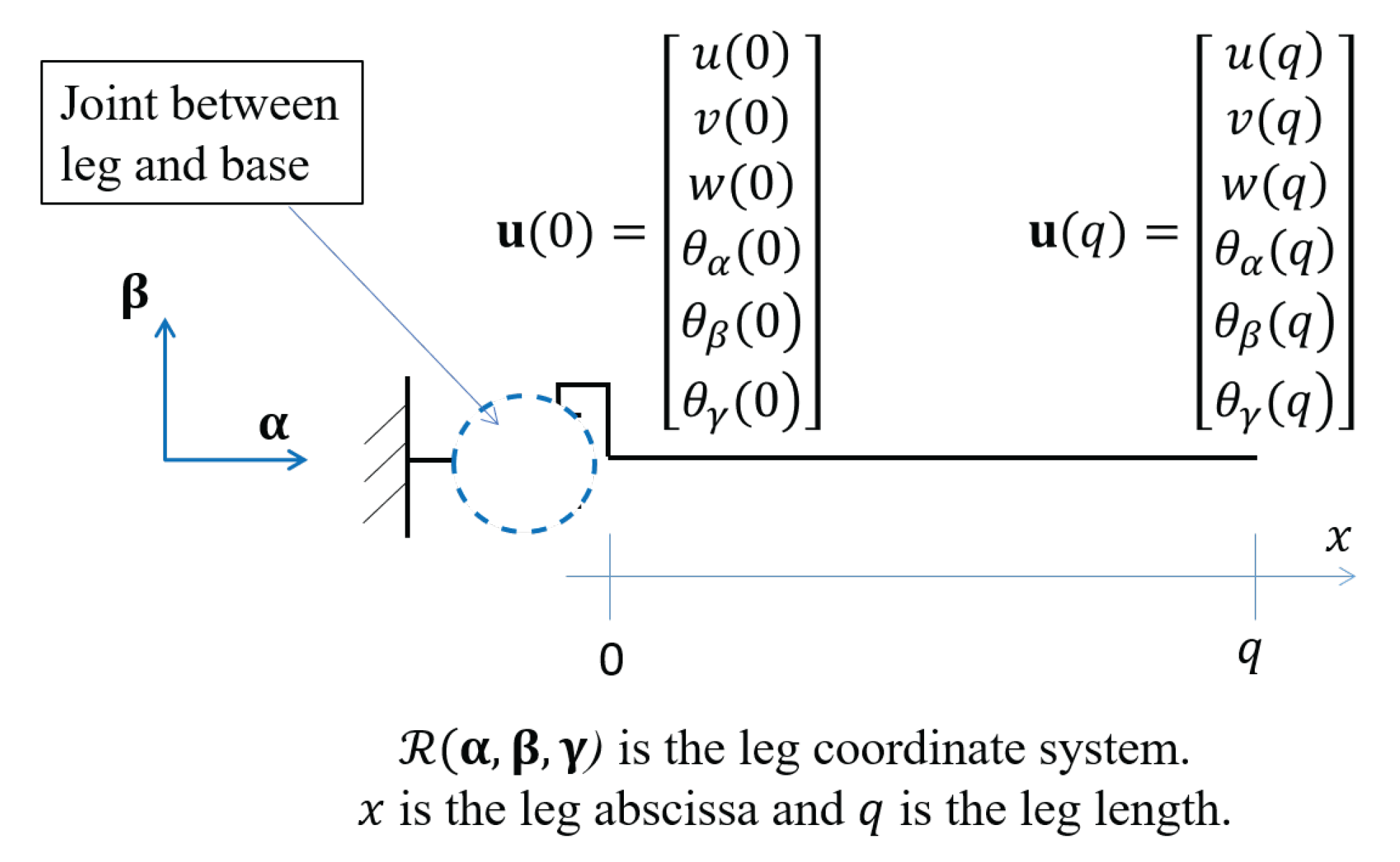
First, each leg is modeled assuming the usual Euler-Bernoulli beam theory. It is worth noting that this model considers the usual mechanical loads, which are bending, traction-compression, and torsion conditions. Each leg is considered to be being connected at one of its ends via a given joint to a fixed part (Figure 4). This boundary condition depends on the joint type used for connecting the leg to the fixed base. In this sub-section, we first study the modeling and the parameter definition of a leg assuming generic boundary conditions to elaborate a leg stiffness matrix and a leg mass matrix in the leg coordinate system. With a generic beam model, leg kinematics are defined through six displacement functions, which correspond to the displacement of the neutral axis. is the vector that collects those displacement functions:
is the displacement along the neutral axis, and are the displacements along fi-direction and fl-direction. , , and correspond to the small rotations about ff-axis, fi-axis and fl-axis, respectively. Using a Bernoulli beam theory, cross-sectional displacements and rotations satisfy the following equations:

Figure 4.
Local leg model and displacement parameters.
Each kinematic function corresponds to a force function. In the following, denotes the force vector and is the moment vector such that:
where is the axial force, and are the shear forces, is the torsion moment, and and are the bending moments. As there is no distributed load, the governing equilibrium equations give:
In addition, the kinematic and force functions are related to each other as follows:
where E is the material Young’s modulus, S is the cross-sectional area, and , and are moments of area about ff-axis, fi-axis and fl-axis.
Combining Equations (2), (4) and (5), we can conclude that and are linear functions, whereas and are polynomial functions of order 3. In a generic case, all kinematic functions can thus be defined through their nodal values expressed in Equation (6).
denotes the vector collecting the nodal values of the kinematic functions (Figure 4) and is expressed as a 1 × 12 column vector:
Vectors , , , , and express the nodal values as a function of x coordinate bounded between 0 and q, i.e., :
From [31], the beam potential energy is written as:
From Equations (8) and (9), can be expressed in a compact form as a function of the beam stiffness matrix and as follows:
With matrix taking the form of Equation (11).
From [31], the beam kinetic energy is defined as:
where is the beam material density, and is the point velocity along the beam expressed as:
Combining Equations (12) and (13) with the hypothesis that -axis and -axis are principal axes of inertia, the kinematic energy writes:
with and the beam inertia about -axis and -axis. Equation (14) takes the following compact form:
with the time derivative of vector and the mass matrix of beam expressed in Equation (16).
with , , and .
To compute the global mass and stiffness matrices, the constraints between the displacements of the leg extremities are determined in the next section.
3.2. Constraint Equations
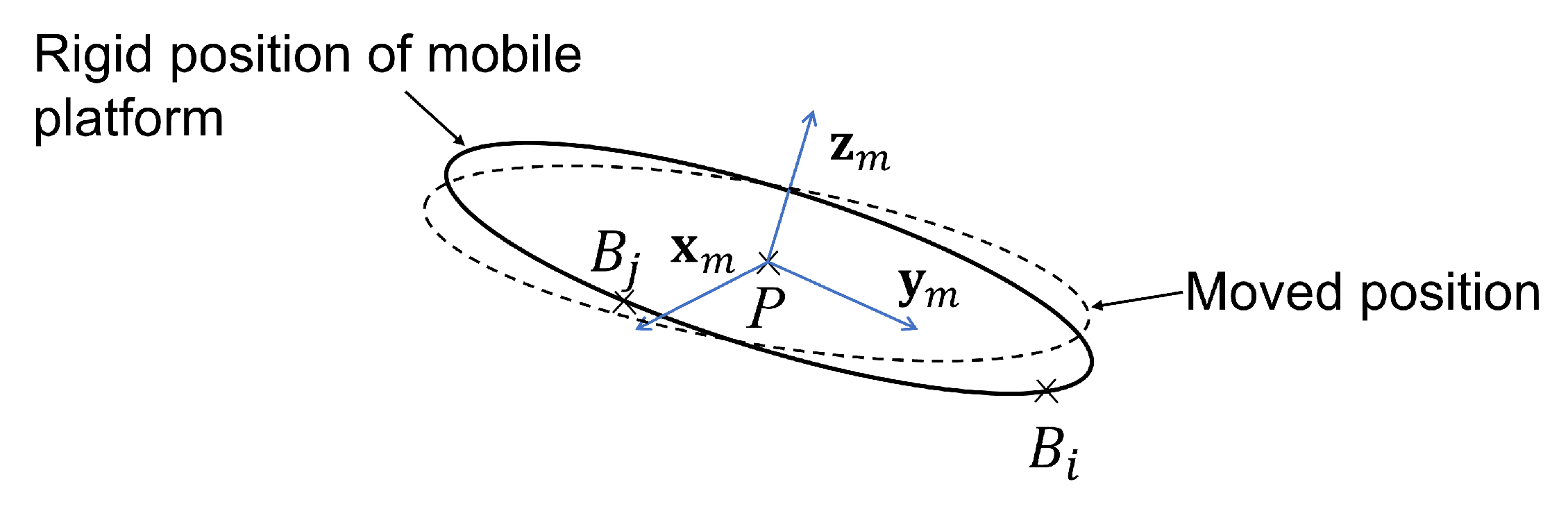
The mobile platform is considered to be rigid for the elaboration of the constraint equations between the leg extremities. We therefore express the movement of the mobile platform due to leg flexibility in stationary configurations of the PKM architecture using screw theory [26] (Figure 5).
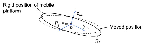
Figure 5.
Parametrization of mobile platform small displacement.
The small displacement screw of the mobile platform is influenced by displacement and rotation of the leg i at point regarding the movements of passive joints between leg i and mobile platform. A normalized screw is used to model passive joint movement [32]. Each movement between leg i and mobile platform is model with a one-DoF motion-screw:
where to ( is the number of equivalent one-DoF joints between leg i and mobile platform, for the case study), is a unit vector along the axis of the screw , is a vector directed from any point on the screw axis to point .
The computation of the movement transmitted by the leg to the mobile platform or vice versa can be done using the reciprocal screws of the motion-screws . There is a unique normalized reciprocal screw system of order 5 of [32]. For a rotational joint, the reciprocal system is a 5-system which includes all rotational screws whose axes intersect the joint axis and all prismatic screws whose axes are perpendicular to joint axes and all the combinations of the above reciprocal screw [32]. The relation between screw and the five one-DoF reciprocal screws is:
where is the identity matrix, is the zero matrix, j = 1 to 5. Then, .
The small displacement screw is defined as with the rotation vector of the mobile platform and the small displacement vector of point ( with the vector from to ). For leg i, the relation between and is written:
where is the rotational matrix between the beam coordinate system and the leg i coordinate system, and is the rotational matrix between the leg i coordinate system and the mobile platform coordinate system.
Constraint equations are defined by expressing Equation (19) for each leg and using small displacement screw properties.
In the same way, the nodal displacement is limited due to passive joints between the leg i and the fixed base. We note the movement-screws between leg i and fixed base. Thus, the null nodal parameter is computed from:
where is the number of equivalent one DoF joints between leg i and fixed base. For the case study, , .
From Equations (19) and (20), constraint equations are grouped together as:
where is a vector composed of the set of beam nodal dependent parameters extracted from all . Its size is equal to the rank of the equation system (19) for all legs. is a vector composed of the set of beam nodal independent parameters, which is not included in . The choice of and is not unique. The components of matrices and are the factor of vectors and components in Equations (19) and (20).
Equation (21) corresponds to a simple formulation of the closed-loop geometric constraints for over-constrained PKM and is the major contribution of the paper. The determination of stiffness and vibratory behavior of a PKM is based on the definition of its global mass and stiffness matrices. These matrices are defined in the following section.
3.3. Mass Matrix Computation of Mobile Platform
The mobile platform and the serial wrist are considered to be a point-mass m located at its center of mass G. Thus, kinematic energy writes:
being the linear velocity of point G. Under the assumption of small displacement is expressed as:
where is the small displacement of point G, is its time derivative and is the vector from G to .
Equation (23) allows defining according to beam nodal parameters:
where is the mobile platform mass matrix. To compute natural frequency of the system, this mass matrix is added to the legs mass matrix.
3.4. Cartesian Stiffness Computation
is the global stiffness matrix of the PKM. It is obtained from the assembly of stiffness matrices of the three legs such that:
where is the stiffness matrix corresponding to dependent beam nodal parameters , and corresponds to the independent ones . is the coupling matrix.
From Equation (21), a decomposition between dependent and independent beam nodal parameters is used to express the potential energy :
Consequently, this allows the introduction of the condensed matrix form of the global stiffness matrix of the studied PKM, which now only depends on the independent beam nodal parameters, such that:
The Cartesian stiffness matrix can be introduced from the expression of the potential energy according to:
where is the small displacement vector of point expressed in the base frame. Thus, where is the rotation matrix from the base frame to the mobile platform frame and is the vector from to . Finally, the Cartesian stiffness matrix of the PKM is computed from :
Note that is a matrix and its components are the stiffness along the PKM base frame vectors.
3.5. Natural Frequency Computation
The global stiffness matrix of the PKM is obtained from the assembly of the mass matrices and of the three legs and mobile platform, respectively. It is expressed as:
where is the mass matrix corresponding to dependent beam nodal parameters , whereas corresponds to the independent ones . is the coupling matrices.
The decomposition between dependent and independent parameters is used to express the kinetic energy as follows:
Consequently, this allows the introduction of the condensed matrix form of the global mass matrix , which now only depends on the independent beam nodal parameters:
The eigenvalues and the associated eigenvector are determined from the spectral decomposition of matrix . The eigenvalues are the solutions of the polynomial . The ith natural frequency is expressed as a function of the ith eignevalue as follows: . The natural modes are the eigenvectors associated with those natural eigenvalues.
4. Natural Frequencies and Modes of Tripteor X7
The methodology described in Section 3 is applied in this section to calculate the natural frequencies and associated modes of the Tripteor X7 PKM.
4.1. Identification of Null Legs Nodal Parameters
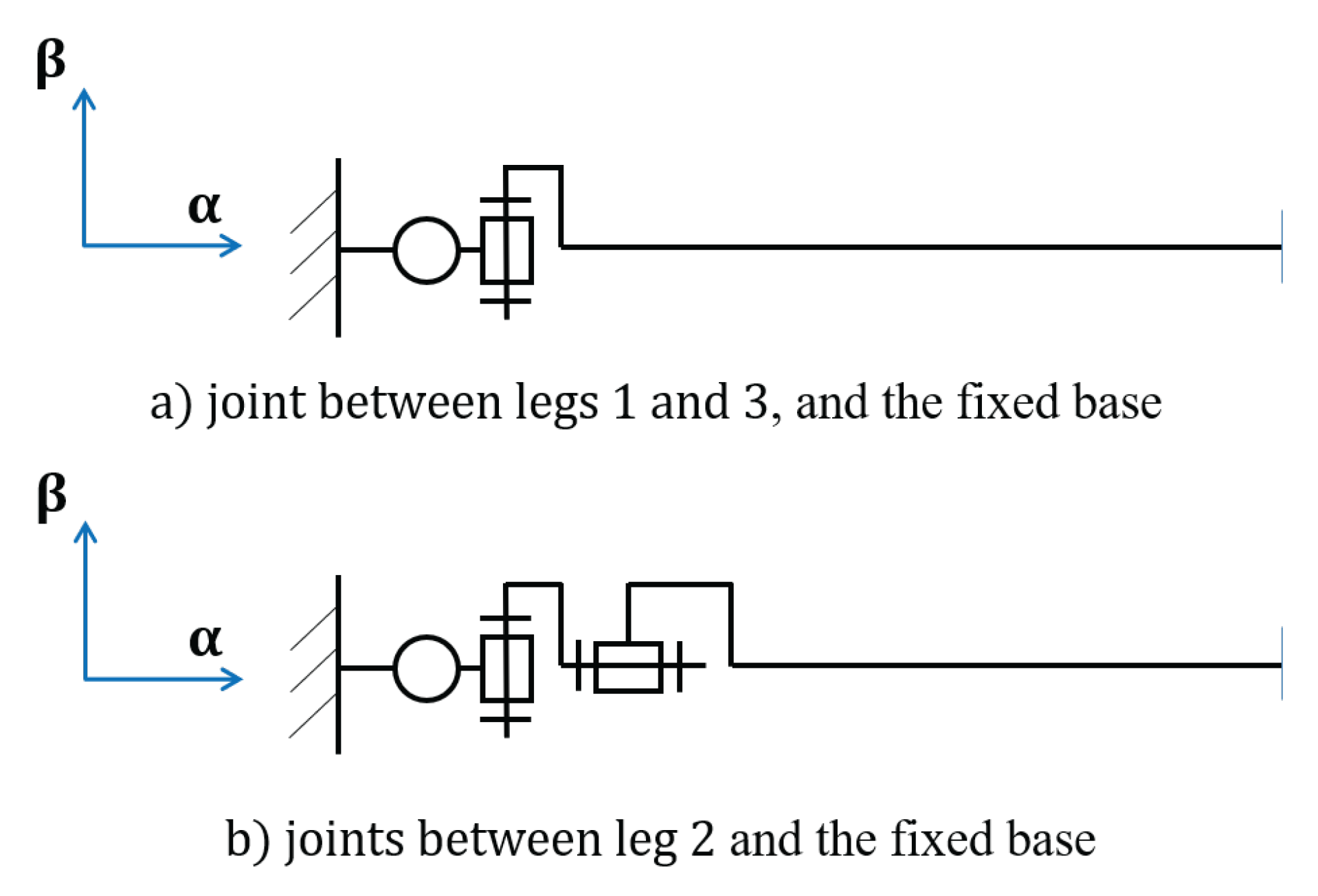
The null nodal parameters of depend on the joint types between the legs and the base as shown in Figure 6. The first joint of Legs 1 and 3 with the base is a revolute joint about -axis, and the second joint is about -axis. Thus, for Legs 1 and 3, infinitesimal and reciprocal screw motion are the following:
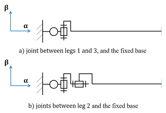
Figure 6.
Local parameters for Tripteor X7 legs.
Thus, from Equation (20), only and are not null.
For Leg 2, with the same methodology, we obtain that only , and are not null (Figure 6b).
To compute the global mass and stiffness matrices, the motion constraints between the extremities of the three legs are explained hereafter.
4.2. Constraint Equations
The joints between Legs 1 and 3 and the mobile platform are revolute joints about -axis (-axis) and the joint between Legs 2 and the mobile platform is a revolute joint about -axis (-axis) (Figure 7). Thus, the reciprocal motion-screws in the leg coordinate system are:
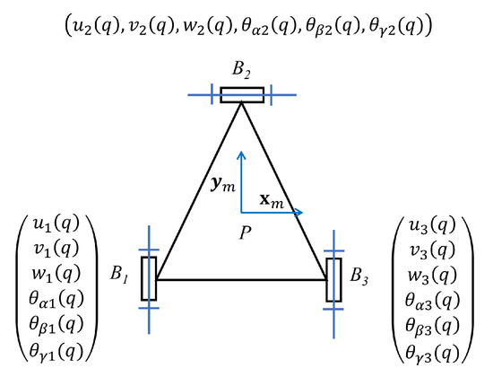
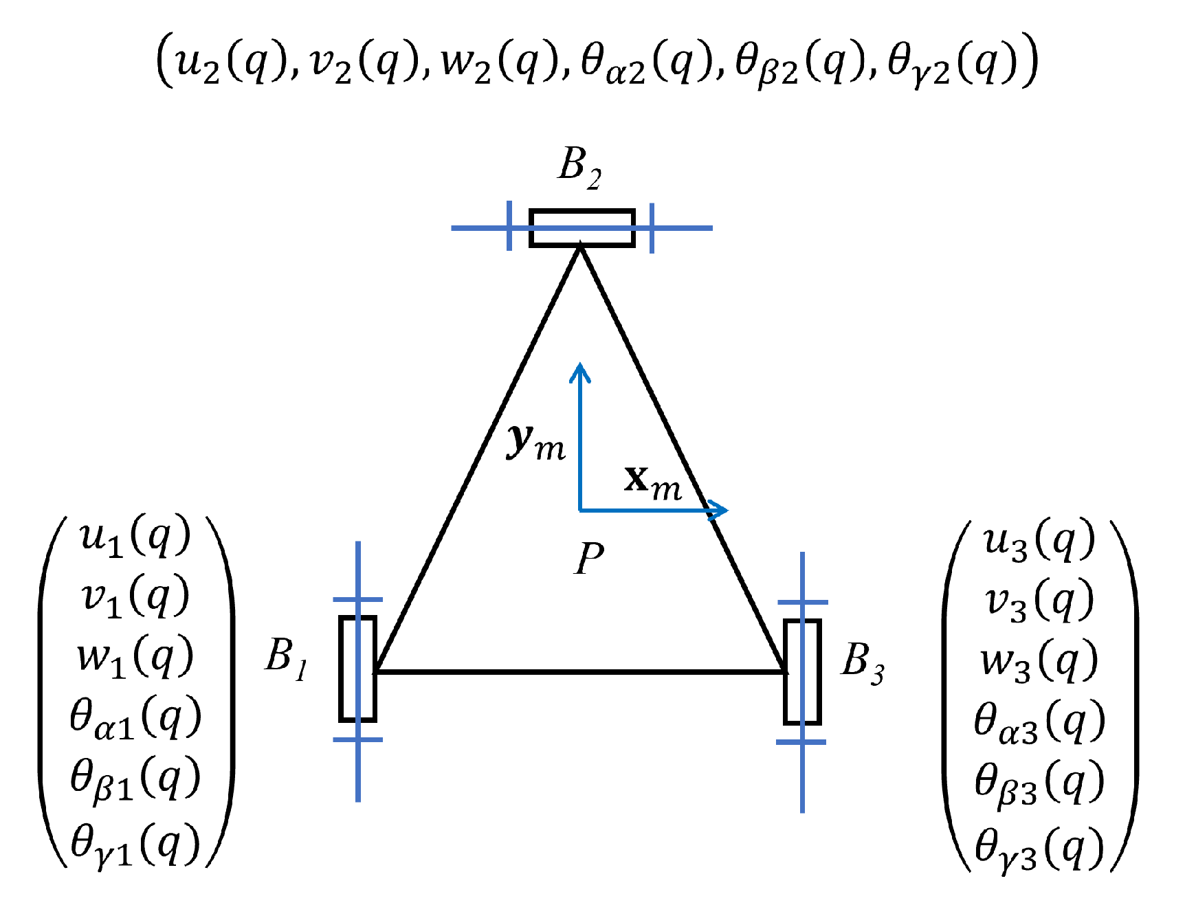
Figure 7.
Parametrization of Tripteor mobile platform movement.
From Equation (19), the equation associated with the motion constraints between the mobile platform and the three legs of Tripteor X7 are the following:
(resp. and ) is the unit vector along the direction of the ith prismatic joint, as shown in Figure 8. The rotation matrix between the beam coordinate system and the leg coordinate system is expressed as:
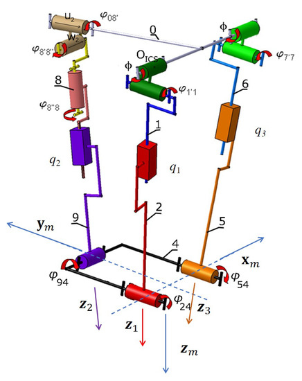
Figure 8.
Leg and mobile platform coordinate systems and joint parametrization of Tripteor X7.
The angles between the legs and the mobile platform are , and (Figure 8). These angles can be measured with a CAD model or computed with the geometric model of the Tripteor PKM described in [33]. With this notation, the rotation matrices between Legs 1, 2 and 3 and the mobile platform coordinate system are:
Consequently, in the case of Tripteor X7, by the application of a small-displacement screw relation at point and from Equations (35)–(37), nine constraint equations are obtained. Nine dependent parameters are chosen:
Thus, 16 independent parameters are considered:
4.3. Cartesian Stiffness Matrix
As discussed in Section 2, Tripteor X7 is modeled as a structural assembly of three legs, which link the rigid fixed platform to the rigid mobile platform. The three legs are considered to be steel beams of rectangular cross-section of size consistent with Tripteor X7 legs (Figure 9).
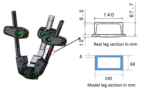
Figure 9.
CAD model of the Tripteor X7 PKM and cross-section of its first leg.
To compute the Cartesian stiffness matrix of the robot at point , the issue is to compute matrix (Equation (29)). Finally, we can compute the stiffness map at a level m for example (Figure 10).
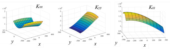
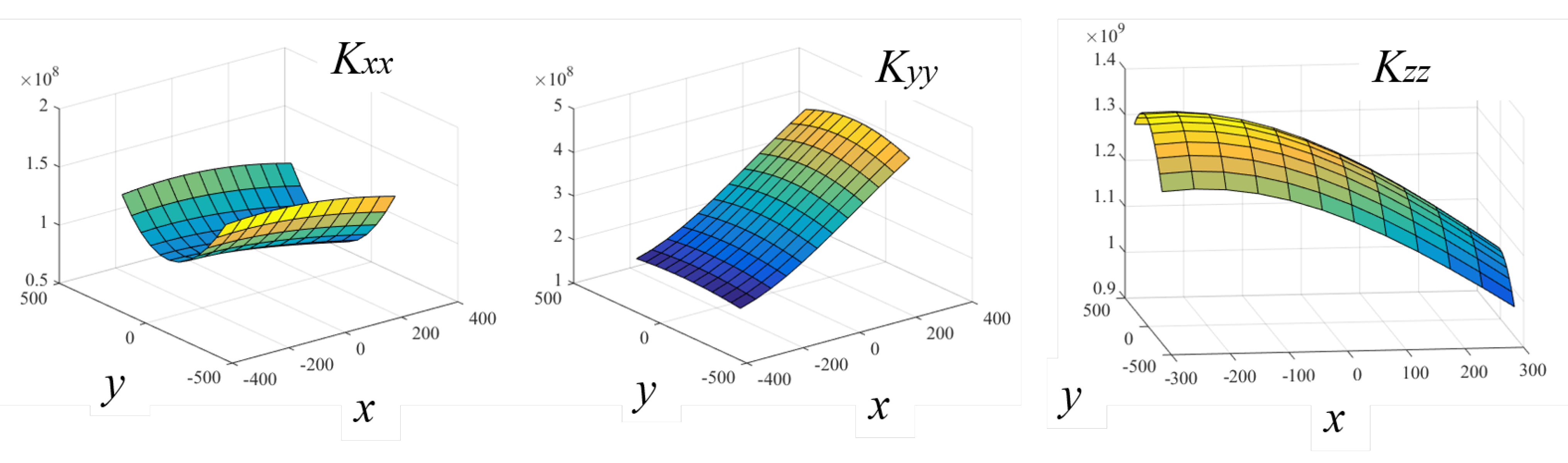
Figure 10.
Principal stiffness coefficients of the Tripteor X7 along X, Y and Z axes in the XY−plane, m.
To plot Figure 11, the method was implemented in Matlab®. To emphasize the benefit of this proposed approach, the calculation was performed on a tablet PC with a I5-7300U processor. The time taken to compute this map is 128.72 s and is mainly due to the time needed to calculate the Inverse Kinematic Model (IKM) of Tripteor X7.
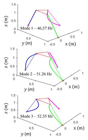
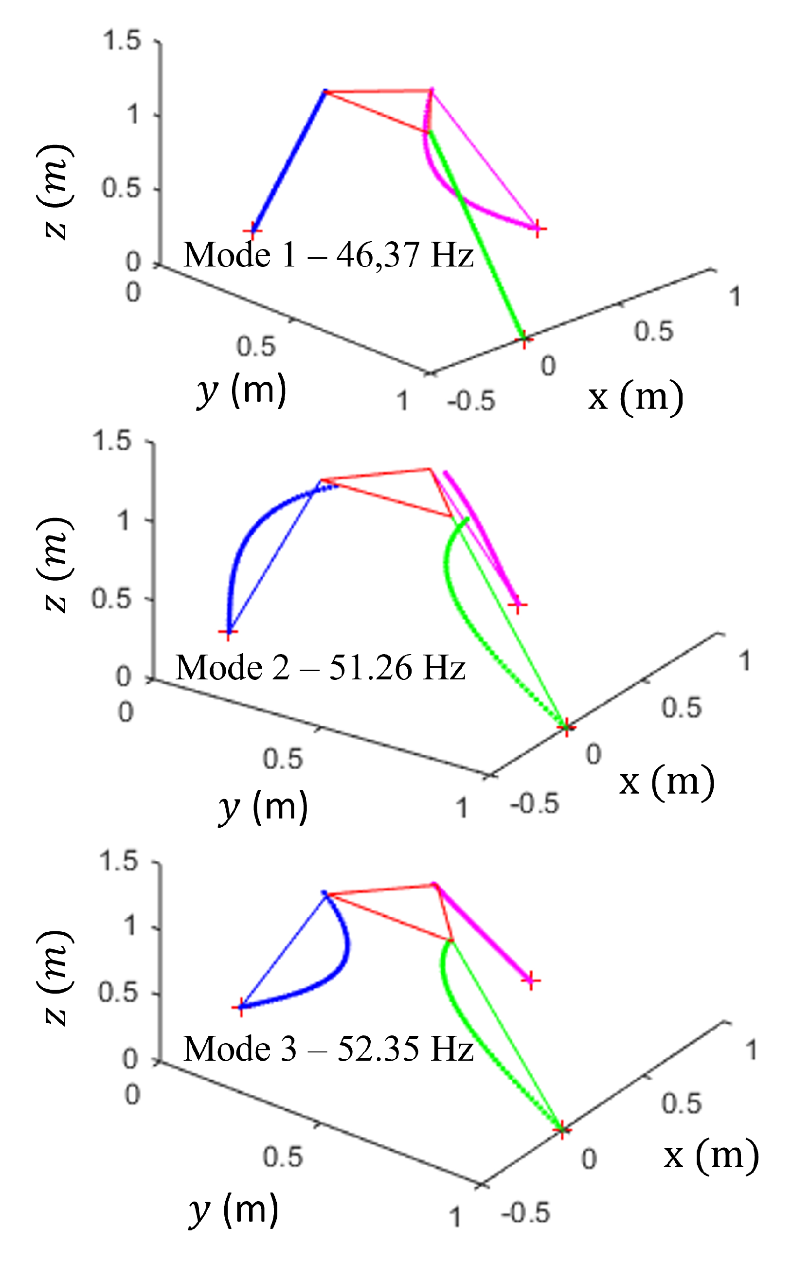
Figure 11.
Modal shapes associated with the first tree natural frequencies of Tripteor X7.
The main advantage of the method is the fast calculation of the natural frequencies and associated modes of over-constrained parallel robots.
4.4. Natural Frequencies
The proposed method is used for the calculation, with a low computational cost, of the first natural frequencies and associated natural modes of the Tripteor X7 PKM.
For this first computation, the leg lengths are m, m and m, and the mass of the mobile platform is considered to be 8 kg. The approach introduced in Section 3 is applied that gives the following estimations for the first natural frequencies in 0.4 s:
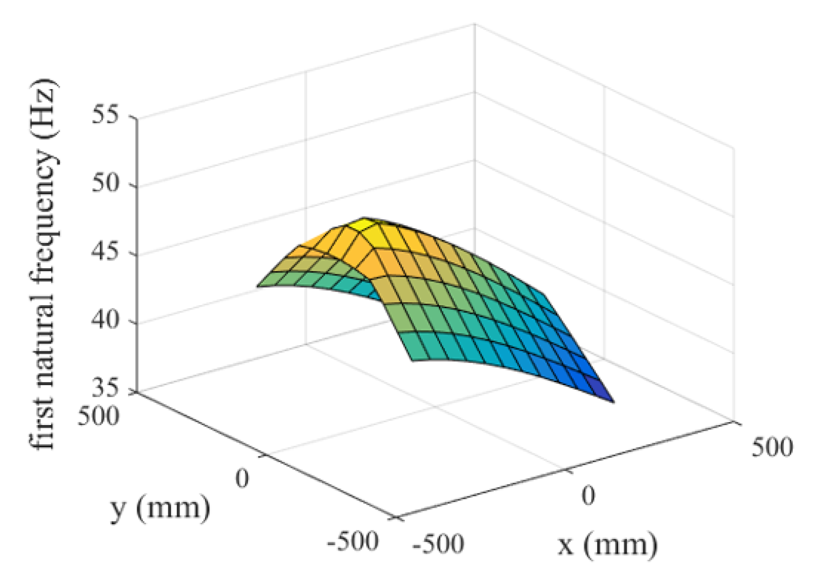
The associated modes of the first three natural frequencies given in Equation (46) are schematized in Figure 11. The variation of first natural frequency value at a level m is illustrated in Figure 12.

Figure 12.
Variation of the first natural frequency.
4.5. Comparison with Experimental Results
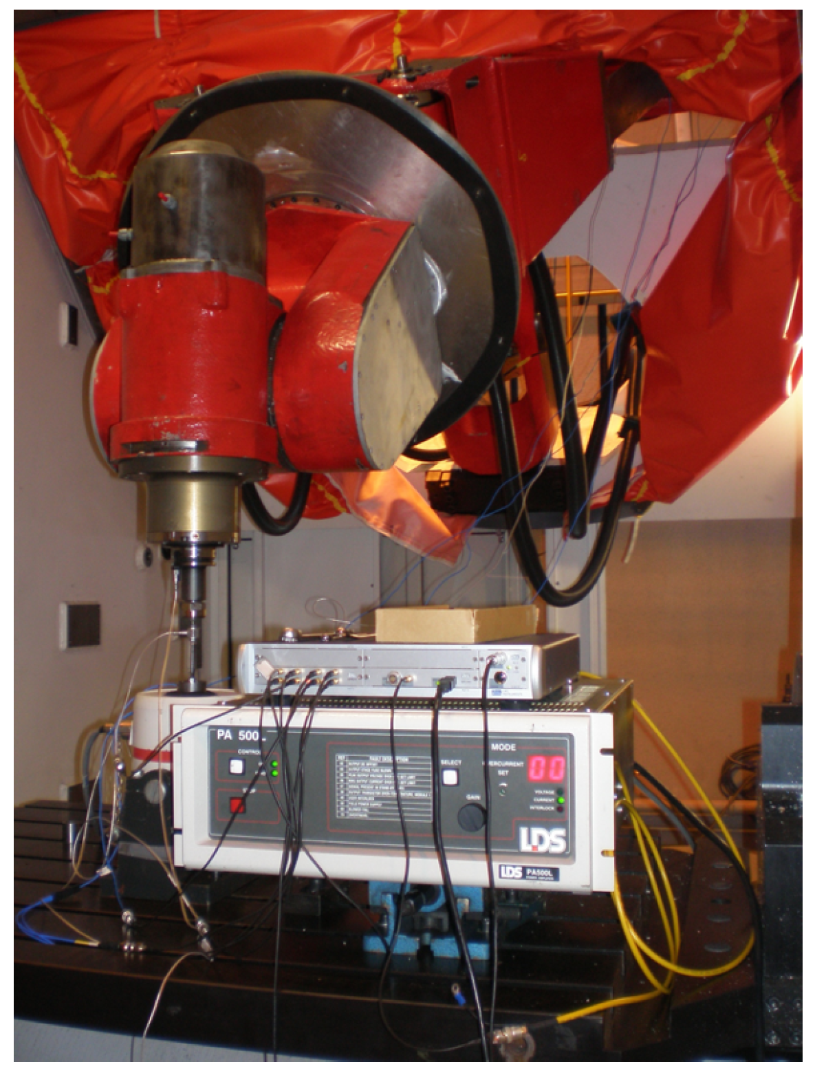
In the literature, previous works studied the modal analysis of the Tripteor X7 PKM architecture using a shaker in three configurations [34] (Figure 13). The displacements of several points of the PKM architecture are measured with accelerometers located on the legs, and on the spindle. Nine DoF are considered for each leg, eight about -axis or -axis and one about -axis, and four DoF for the spindle (Figure 14). The obtained results show four natural frequencies close to 40, 50, 70 and 90 Hz.

Figure 13.
First natural frequency measurement.
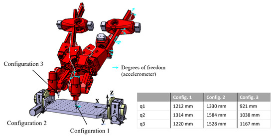
Figure 14.
Configuration of the Tripteor X7 for the experimental measurement.
The same configurations 1, 2 and 3 were considered with the proposed beam approach, and the associated results are given in Table 1. Experimental and simulated results are close for the first mode. For the other modes, the simplification of the legs modeling and the difference of mass distribution between the model and the real machine tool can explain the gap between estimated and measured natural frequencies. Indeed, the modeling of the leg under the assumption that their cross-section area is constant affects the leg stiffness, inertia and the position of its gravity center. This impact is different regarding the leg lengths and so to the studied configuration. It should be noted that this method is dedicated to the embodiment design of parallel manipulators. Therefore, such an error is acceptable, and the simplification of the leg shape allows the reduction of the calculation time of the elasto-dynamic model.

Table 1.
Comparison of measured natural frequencies and calculated ones with the proposed method.
5. Conclusions
This paper described a new methodology to compute the first natural frequencies of over-constrained PKMs based on the application of screw theory under the assumption of small displacements. Specifically designed to require few computing resources, the obtained model enables the estimation of stiffness maps, first natural frequencies and associated modes in a simple way without computing any Jacobian matrix. The proposed methodology was validated by comparing the obtained theoretical natural frequencies and associated modes of the Tripteor X7 to the measured experimental values. Errors between experimental and simulated results are less than 13% for the first mode and 33% for the second and third modes.
As a conclusion, the proposed methodology allows the mathematical expression of the simplified elasto-dynamic model of over-constrained parallel robots to reduce considerably the computation time of their natural frequencies. This low computation time allows the designer of over-constrained parallel robots to quickly estimate the natural frequencies of candidate robot architectures at the conceptual design stage and thus make the right choices of robot architecture with respect to required elasto-dynamic performance and a given task.
Later, variations in leg cross-sections will be implemented and joint stiffness will be added as an additional stiffness at beam extremities.
Author Contributions
Conceptualization, H.C., A.G., B.B. and S.C.; methodology, H.C. and S.C.; validation, H.C.; formal analysis, H.C., B.B. and S.C.; writing—original draft preparation, H.C.; writing—review and editing. All authors have read and agreed to the published version of the manuscript.
Funding
This research received no external funding.
Acknowledgments
This work was carried out within the Manufacturing 21 working group, which comprises 18 French research laboratories. The topics approached are: modeling of the manufacturing process, virtual machining, emergence of new manufacturing methods.
Conflicts of Interest
The authors declare no conflict of interest.
Abbreviations
The following abbreviations are used in this manuscript:
| ith joint variable | |
| x | Beam abscissa |
| Displacement vector of the beam neutral axis | |
| Vector collecting the nodal values of the kinematic functions | |
| Beam displacement along the neutral axis | |
| Beam displacement along -axis | |
| Beam displacement along -axis | |
| Beam section rotation about neutral axis | |
| Beam section rotation about -axis | |
| Beam section rotation about -axis | |
| Beam force vector at a given abscissa | |
| Beam moment vector at a given abscissa | |
| Beam stiffness matrix | |
| Beam mass matrix | |
| Vector of small displacements of point | |
| Rotation vector of the mobile platform | |
| Vector of dependent parameters | |
| Vector of independent parameters | |
| Global stiffness matrix | |
| Global mass matrix | |
| First natural frequency vector |
References
- Patel, Y.; George, P. Parallel manipulators applications—A survey. Mod. Mech. Eng. 2012, 2, 57. [Google Scholar] [CrossRef] [Green Version]
- Li, Y.; Ma, Y.; Liu, S.; Luo, Z.; Mei, J.; Huang, T.; Chetwynd, D. Integrated design of a 4-DOF high-speed pick-and-place parallel robot. CIRP Ann. 2014, 63, 185–188. [Google Scholar] [CrossRef]
- Chanal, H.; Duc, E.; Ray, P. A study of the impact of machine tool structure on machining processes. Int. J. Mach. Tools Manuf. 2006, 46, 98–106. [Google Scholar] [CrossRef]
- Terrier, M.; Dugas, A.; Hascoet, J.Y. Qualification of parallel kinematics machines in high-speed milling on free form surfaces. Int. J. Mach. Tools Manuf. 2004, 44, 865–877. [Google Scholar] [CrossRef]
- Pritschow, G.; Eppler, C.; Garber, T. Influence of the dynamic stiffness on the accuracy of PKM. In Proceedings of the Chemnitz Parallel Kinematic Seminar, Chemnitz, Germany, 23–25 April 2002; pp. 313–333. [Google Scholar]
- Pateloup, S.; Chanal, H.; Duc, E. Process parameter definition with respect to the behaviour of complex kinematic machine tools. Int. J. Adv. Manuf. Technol. 2013, 69, 1233–1248. [Google Scholar] [CrossRef]
- Neumann, K. Exechon concept-parallel kinematic machines in research and practice. In Proceedings of the Chemnitz Parallel Kinematics Seminar, Chemnitz, Germany, 25–26 April 2006. [Google Scholar]
- IFToMM. IFToMM Dictionnary—3. Dynamics. Available online: http://www.iftomm-terminology.antonkb.nl/2057_1036/frames.html (accessed on 6 March 2022).
- Liu, W.L.; Xu, Y.D.; Yao, J.T.; Zhao, Y.S. Methods for force analysis of overconstrained parallel mechanisms: A review. Chin. J. Mech. Eng. 2017, 30, 1460–1472. [Google Scholar] [CrossRef] [Green Version]
- Mei, B.; Xie, F.; Liu, X.J.; Yang, C. Elasto-geometrical error modeling and compensation of a five-axis parallel machining robot. Precis. Eng. 2021, 69, 48–61. [Google Scholar] [CrossRef]
- Benti, A.; Durieux, S.; Chanal, H. Mesure du Comportement Vibratoire D’une Machine-Outil à Structure Parallèle. 8ème Assises MUGV 2014. Available online: https://tel.archives-ouvertes.fr/tel-00451081/document (accessed on 9 March 2022).
- Pierrot, F.; Pierrot, F. Modelling and design issues of a 3-axis parallel machine-tool. Mech. Mach. Theory 2002, 11, 1325–1345. [Google Scholar]
- Yan, S.; Ong, S.; Nee, A. Stiffness analysis of parallelogram-type parallel manipulators using a strain energy method. Robot. Comput.-Integr. Manuf. 2016, 37, 13–22. [Google Scholar] [CrossRef]
- Wang, Y.; Huang, T.; Zhao, X.; Mei, J.; Chetwynd, D.G.; Hu, S.J. Finite element analysis and comparison of two hybrid robots-the tricept and the trivariant. In Proceedings of the 2006 IEEE/RSJ International Conference on Intelligent Robots and Systems, Beijing, China, 9–15 October 2006; pp. 490–495. [Google Scholar]
- Klimchik, A.; Pashkevich, A.; Chablat, D. CAD-based approach for identification of elasto-static parameters of robotic manipulators. Finite Elem. Anal. Des. 2013, 75, 19–30. [Google Scholar] [CrossRef] [Green Version]
- Germain, C.; Briot, S.; Caro, S.; Wenger, P. Natural frequency computation of parallel robots. J. Comput. Nonlinear Dyn. 2015, 10, 021004. [Google Scholar] [CrossRef]
- Zhang, J.; Zhao, Y.Q.; Jin, Y. Elastodynamic modeling and analysis for an Exechon parallel kinematic machine. J. Manuf. Sci. Eng. 2016, 138, 031011. [Google Scholar] [CrossRef]
- Kermanian, A.; Kamali, A.; Taghvaeipour, A. Dynamic analysis of flexible parallel robots via enhanced co-rotational and rigid finite element formulations. Mech. Mach. Theory 2019, 139, 144–173. [Google Scholar] [CrossRef]
- Klimchik, A.; Pashkevich, A.; Chablat, D. Fundamentals of manipulator stiffness modeling using matrix structural analysis. Mech. Mach. Theory 2019, 133, 365–394. [Google Scholar] [CrossRef]
- Guo, J.; Zhao, Y.; Chen, B.; Zhang, G.; Xu, Y.; Yao, J. Force Analysis of the Overconstrained Mechanisms Based on Equivalent Stiffness Considering Limb Axial Deformation. Res. Sq. 2021. Available online: https://www.researchsquare.com/article/rs-634709/v1 (accessed on 6 March 2022). [CrossRef]
- Yang, C.; Li, Q.; Chen, Q.; Xu, L. Elastostatic stiffness modeling of overconstrained parallel manipulators. Mech. Mach. Theory 2018, 122, 58–74. [Google Scholar] [CrossRef]
- Bi, Z. Kinetostatic modeling of Exechon parallel kinematic machine for stiffness analysis. Int. J. Adv. Manuf. Technol. 2014, 71, 325–335. [Google Scholar] [CrossRef]
- Bi, Z.M.; Jin, Y. Kinematic modeling of Exechon parallel kinematic machine. Robot. Comput.-Integr. Manuf. 2011, 27, 186–193. [Google Scholar] [CrossRef]
- Amine, S.; Caro, S.; Wenger, P. Constraint and singularity analysis of the Exechon. Appl. Mech. Mater. 2012, 162, 141–150. [Google Scholar] [CrossRef]
- Selig, J.; Ding, X. A screw theory of timoshenko beams. J. Appl. Mech. 2009, 76, 031003. [Google Scholar] [CrossRef]
- Bourdet, P.; Mathieu, L.; Lartigue, C.; Ballu, A. The concept of small displacement torsor in metrology. Ser. Adv. Math. Appl. Sci. 1996, 40, 110–122. [Google Scholar]
- Aydin, Y.; Kucuk, S. Quaternion based inverse kinematics for industrial robot manipulators with Euler wrist. In Proceedings of the 2006 IEEE International Conference on Mechatronics, Budapest, Hungary, 3–5 July 2006; pp. 581–586. [Google Scholar]
- Bonnemains, T.; Chanal, H.; Bouzgarrou, B.C.; Ray, P. Stiffness computation and identification of parallel kinematic machine tools. J. Manuf. Sci. Eng. 2009, 131, 041013. [Google Scholar] [CrossRef]
- Klimchik, A.; Pashkevich, A.; Caro, S.; Chablat, D. Stiffness modeling of robotic-manipulators under auxiliary loadings. International Design Engineering Technical Conferences and Computers and Information in Engineering Conference. Am. Soc. Mech. Eng. 2012, 45035, 469–476. [Google Scholar]
- Kucuk, S. Dexterous workspace optimization for a new hybrid parallel robot manipulator. J. Mech. Robot. 2018, 10, 064503. [Google Scholar] [CrossRef]
- Yoo, H.; Ryan, R.; Scott, R.A. Dynamic of flexible beams undergoing overall motions. J. Sound Vib. 1995, 181, 261–278. [Google Scholar] [CrossRef]
- Kong, X.; Gosselin, C.M. Type Synthesis of Parallel Mechanisms; Springer: Berlin/Heidelberg, Germany, 2007; Volume 33. [Google Scholar]
- Pateloup, S.; Chanal, H.; Duc, E. Geometric and kinematic modelling of a new Parallel Kinematic Machine Tool: The Tripteor X7 designed by PCI. Adv. Mater. Res. 2010, 112, 159–169. [Google Scholar] [CrossRef]
- Bonnemains, T.; Chanal, H.; Bouzgarrou, B.C.; Ray, P. Dynamic analysis of the Tripteor X7: Model and experiments. Robot. Comput.-Integr. Manuf. 2010, 29, 180–191. [Google Scholar] [CrossRef]


Publisher’s Note: MDPI stays neutral with regard to jurisdictional claims in published maps and institutional affiliations. |
© 2022 by the authors. Licensee MDPI, Basel, Switzerland. This article is an open access article distributed under the terms and conditions of the Creative Commons Attribution (CC BY) license (https://creativecommons.org/licenses/by/4.0/).